the Creative Commons Attribution 4.0 License.
the Creative Commons Attribution 4.0 License.
 | 07 Jul 2021
Nonstationary weather and water extremes: a review of methods for their detection, attribution, and management
Louise J. Slater
Bailey Anderson
Marcus Buechel
Simon Dadson
Shasha Han
Shaun Harrigan
Timo Kelder
Katie Kowal
Thomas Lees
Tom Matthews
Conor Murphy
Robert L. Wilby
Hydroclimatic extremes such as intense rainfall, floods, droughts, heatwaves, and wind or storms have devastating effects each year. One of the key challenges for society is understanding how these extremes are evolving and likely to unfold beyond their historical distributions under the influence of multiple drivers such as changes in climate, land cover, and other human factors. Methods for analysing hydroclimatic extremes have advanced considerably in recent decades. Here we provide a review of the drivers, metrics, and methods for the detection, attribution, management, and projection of nonstationary hydroclimatic extremes. We discuss issues and uncertainty associated with these approaches (e.g. arising from insufficient record length, spurious nonstationarities, or incomplete representation of nonstationary sources in modelling frameworks), examine empirical and simulation-based frameworks for analysis of nonstationary extremes, and identify gaps for future research.


Are hydroclimatic extremes stationary or nonstationary? This question has generated much debate because of the ramifications for hazard management in a changing world. At the simplest level, a stationary process is one in which the statistical properties of the distribution and correlation do not shift over time. Thus, a stationary time series (Fig. 1a) would not exhibit any shift in mean, variance (Fig. 1b), or shape. For hydroclimatic extremes, this implies that the distribution of extreme precipitation, temperature, streamflow, or wind should merely fluctuate within a stationary envelope of variability. The assumption of stationarity has long served as the basis for the statistical analysis of hazards and the design of engineering structures, by defining the magnitude of events with a given frequency of occurrence, such as the stationary 100-year design flood (e.g. Salas et al., 2018).
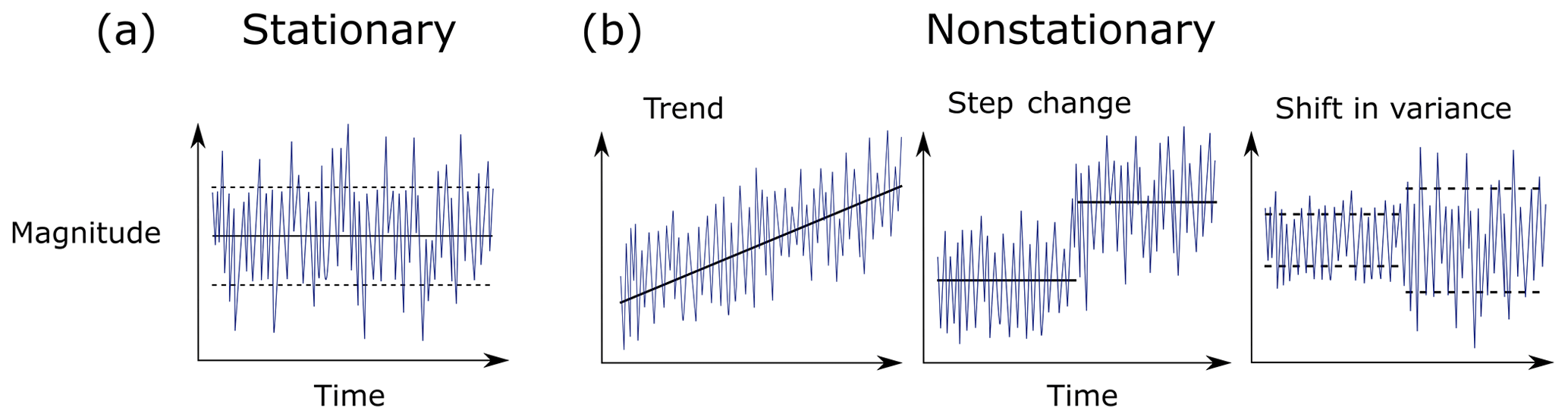
Figure 1What is nonstationarity? Examples of (a) a stationary time series with constant mean and variance and (b) three nonstationary time series in the form of a shift in mean (trend and step change) and a shift in variance. Solid and dashed black lines represent the mean and the variance of the time series, respectively.
In reality, the global water cycle manifests many artificial patterns and trends induced by human activities such as climate change, land cover change (e.g. Blum et al., 2020), water abstraction or augmentation, river regulation, and even geopolitical uncertainty (e.g. Wine, 2019) at local, regional, and global scales. Trends and step changes in the magnitude, frequency, duration, volume, or areal extent of hydroclimatic extremes, such as intense rainfall (e.g. Sun et al., 2020a; Westra et al., 2013; Donat et al., 2016), floods (e.g. Berghuijs et al., 2019a; Do et al., 2017; Archfield et al., 2016), droughts (e.g. Andreadis and Lettenmaier, 2006; Spinoni et al., 2017), and heatwaves or heat stress (e.g. Oliver et al., 2018; Lorenz et al., 2019; Ouarda and Charron, 2018), have been widely detected and have led to proclamations about the “death” of stationarity in water management (Milly et al., 2008). In contrast, trends in strong winds or storms are less certain, and the influence of anthropogenic climate change is difficult to attribute (Shaw et al., 2016; Elsner et al., 2008; Martínez-Alvarado et al., 2018; Wohland et al., 2019). Disentangling natural and anthropogenic drivers of nonstationarity is problematic as the two can be interlinked, and even seemingly “natural” drivers such as climate modes may shift under the effects of anthropogenic climate change (e.g. Maher et al., 2018). Although the drivers of abrupt nonstationarities (step changes) may be apparent (e.g. water abstraction, reservoir filling, and operations), drivers of more incremental nonstationarities (trend or variance; e.g. climate variability and change and land cover change) may be harder to attribute and/or obfuscated by other confounding factors.
Deciding whether to employ nonstationary methods for the purpose of managing extremes is thus a key challenge facing weather and water scientists and practitioners today (e.g. Faulkner and Sharkey, 2020), as it is unclear how to represent increased uncertainty arising from climate change (e.g. Wasko et al., 2021). Detecting the presence, and attributing the source of nonstationarity in hydroclimatic extremes, is, however, vital for understanding and managing water resources in a changing world. Nonstationarity may have dramatic impacts for infrastructure (François et al., 2019), property, and society over a range of overlapping timescales. There are many different drivers that may alter extremes simultaneously over both the short term (such as human management impacts) and medium to long term (such as land cover and climate change impacts) (e.g. Warner, 1987; Rust et al., 2019). Short-term trends are widely present in variables like streamflow, which exhibit long memory (time dependence) and periodicities. However, such trends are not necessarily indicative of nonstationarity (e.g. Koutsoyiannis, 2006; Koutsoyiannis and Montanari, 2015). “Nonsense correlations” can be found between time-varying variables without any physical significance (Yule, 1926), and apparent trends or oscillations may be found in time series due to random causes (Slutzky, 1937). In fact, random fluctuations or deviations from the mean are to be expected in stationary time series (e.g. Wunsch, 1999), especially those with a long memory. Multi-decadal (e.g. 30 year) shifts may simply be temporary excursions in longer (e.g. 100 year) records, or a function of the start and end dates chosen for the trend analysis (Harrigan et al., 2018), and may not warrant the application of nonstationary analysis. A growing body of literature has shown that inappropriately applying nonstationary models to short time series may have the undesired effect of increasing uncertainty; in cases where model structure and/or underlying physical drivers are uncertain, stationary models may be the preferred option for design and management of extremes (Serinaldi and Kilsby, 2015). Nonstationarity should not be presumed to occur everywhere simply because of climate change (Lins, 2012); nonstationary approaches have value primarily when there are good reasons to suspect physically plausible and predictable drivers of change.
Over the last 2 decades, hundreds of papers have addressed the detection, attribution, prediction, and projection of nonstationarity in precipitation, floods, drought, heat stress, temperature, extreme winds, and storms. However, a comprehensive introductory overview of these methods across hydroclimatic extremes, including an overarching discussion of the key challenges that can arise, has not been published to date. This paper is the first to review the entire nonstationary management process, from identifying metrics to analysis through to management. This paper offers a synthesis of methods for quantifying, attributing, and managing nonstationarity over multiple spatial and temporal scales, along with their limitations. The structure follows the logical order of steps employed in a detection, attribution, and management framework (Fig. 2). Challenges are presented for each step throughout the paper.
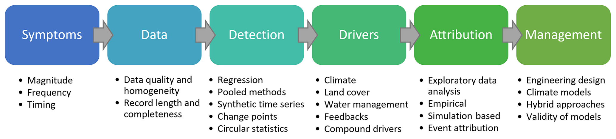
Section 2 describes the most widely used indices for diagnosing the symptoms of nonstationarity via changes in magnitude, frequency, and timing. Section 3 identifies essential data prerequisites for detecting nonstationarity, such as homogeneity analysis. Section 4 discusses the techniques used to detect nonstationarity, including regression-based methods for gradual change, pooled approaches for analysis of rare extremes, step change analysis for abrupt change, and other methods for discerning changing seasonality. Section 5 introduces the key drivers of nonstationarity of hydroclimatic extremes. Section 6 reviews approaches for attribution of nonstationary extremes, including both observation- and model-based approaches, and issues with attribution and engineering design under nonstationarity. Finally, Sect. 7 discusses approaches for managing nonstationarity via engineering design and model projections, including key limitations. The overall aim of the paper is to highlight the most significant issues and considerations when detecting, attributing, predicting, and projecting nonstationarity in hydroclimatic extremes.
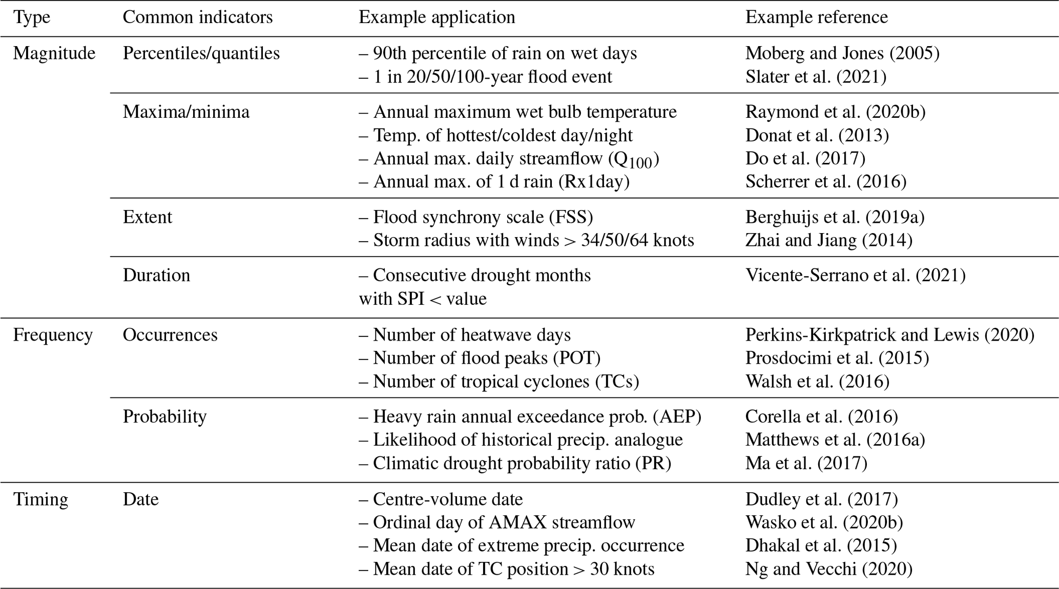
Nonstationarities in hydroclimatic extremes may be expressed through a significant shift in the mean, variance, or shape of a given time series (Fig. 1). Such departures are generally diagnosed by symptoms such as a change in the magnitude (events becoming more or less extreme), frequency (events occurring more or less often than before), and timing (events occurring earlier or later in the year) of seasonal or annual extremes. There are many different ways of describing the symptoms of nonstationarity – each is discussed in turn below, and examples are provided in Table 1.
2.1 Magnitude
Significant changes in the magnitude of extremes are relevant to society, engineers, decision makers, and insurers alike. The magnitude or intensity of an event is generally described by estimating the percentiles of a distribution over a given period. Examples may include the peak rainfall, peak streamflow, peak intensity of a drought, maximum/minimum temperature, or peak wind speed within a given day, month, season, or a year (Fig. 3). Significant changes are detected by evaluating alterations in these percentiles over time (e.g. a time series of annual maximum daily streamflow). More generally, magnitudes can also be described via metrics characterizing the intensity or flashiness of an event, such as its spatial extent, duration, or time to peak (Fig. 3).
The magnitude or intensity of precipitation (in millimetres; Fig. 3a) can be assessed using various metrics. Many of these are part of the ETCCDI indices that were proposed in 2002 by the expert team on climate change detection and indices (ETCCDIs; see, e.g., Frich et al., 2002; Zhang et al., 2011). Precipitation metrics include the maximum depth of precipitation accumulation for a given duration (1, 3, or 6 h and 1 or 5 d, termed Rx1day or Rx5day, respectively) within a given month, season, or year (e.g. Champion et al., 2019; Sun et al., 2020a). This includes the percentage of rain that fell in the monthly maximum 1 h precipitation (or some other period), the 90th, 95th, or 99th percentile precipitation amount (over 1, 3, or 6 h) during a month or year – or, specifically, on wet days (Moberg and Jones, 2005) – or even the total precipitation accumulated from hours exceeding specified percentiles over a month or year (e.g. Donat et al., 2013). For instance, at the global scale, analysis of the Rx1day and Rx5day precipitation accumulations found that extreme precipitation has increased at about two-thirds of stations – a significantly greater proportion than can be expected by chance (Sun et al., 2020a). An important concept is the probable maximum precipitation (PMP), i.e. the greatest depth of precipitation that is possible in a given place and time and for a given storm duration. For a complete state-of-the-art review on the PMP concept, see Salas et al. (2020). PMP can be computed via hydrometeorological, statistical, grid-based, and site-specific approaches, using both stationary and nonstationary methods (e.g. Lee and Singh, 2020). PMP is expected to increase in many regions in future decades due to increases in atmospheric moisture content and moisture transport into storms (Kunkel et al., 2013).

Figure 3Metrics employed for evaluating five types of hydroclimatic extremes. (a) Precipitation hyetograph. (b) Flood hydrograph. (c) Drought. (d) Temperature. (e) Wind (storms). All these variables can be described using indicators of event duration and magnitude (peak intensity).
Percentiles of daily streamflow distribution are commonly used for floods (Fig. 3b). For example, the Q90 (the 90th percentile of the distribution, i.e. the flow that is exceeded 10 % of the time, confusingly referred to as “Q90” in North America and “Q10” in Great Britain and Ireland), Q95, Q99 (flow that is exceeded 3.65 d per year, on average), Q99.9 (0.37 d per year), or AMAX (the annual maximum streamflow). When considering more extreme events than AMAX, hydroclimatic extremes are commonly expressed as 1 in 20-, 1 in 50-, or 1 in 100-year events (e.g. Milly et al., 2002; Slater et al., 2021). Hydrograph analyses may also be used to extract metrics such as flood volume and duration (Fig. 3b). Other indicators describe the flashiness of an event, such as the time to peak, which is defined as the total number of hours starting from the sharp rise of the hydrograph until the peak discharge. The spatial extent of a flood event can be described using metrics such as the number of catchments flooding simultaneously (Uhlemann et al., 2010) or the flood synchrony scale (FSS), which evaluates the largest radius around a stream gauge where more than half of the surrounding stream gauges also record flooding within the same week (Berghuijs et al., 2019a). Studies are increasingly evaluating the spatial dependence of flooding across multiple basins by considering meteorological, temporal, and land surface processes leading to simultaneous flooding across varying spatial scales (e.g. Brunner et al., 2020; Kemter et al., 2020; Wilby and Quinn, 2013).
Droughts (Fig. 3c) differ from other extreme weather because they develop more slowly and last longer; they are broadly defined as “a sustained period of below-normal water availability” (Tallaksen and Van Lanen, 2004) and are sometimes referred to as a “creeping phenomenon” (Mishra and Singh, 2010; Wilhite, 2016). These characteristics make it more difficult to assess nonstationarity as there are fewer events to compare over time; plus, drought onset and termination are challenging to pinpoint (Parry et al., 2016). Not all droughts are defined by aridity, and rainfall deficit alone does not imply a drought (Van Loon, 2015). Instead, a combination of factors in the hydrological cycle interact to yield below-normal conditions (Fig. 3c). Drought has been typically classified as being meteorological (precipitation deficit), hydrological (surface and subsurface water deficit relative to local water uses), agricultural (declining soil moisture and crop failure), or socioeconomic (failure of water resources system to meet demand) (Van Loon, 2015). Since the definition of normal conditions depends on spatial and temporal scales, drought anomalies are typically defined locally, using composite indicators including precipitation and temperature. Various metrics exist to measure drought stress, and they either reflect deficits in precipitation or combined metrics of precipitation, temperature, and evaporation. The World Meteorological Organization (WMO) recommends the use of the Standardized Precipitation Index (SPI), which reflects standard deviations from normal rainfall (WMO, 2016; McKee et al., 1993). Other well-known indices that rely on monthly precipitation include the Palmer drought severity index (PDSI; Palmer, 1965), deciles (Gibbs and Maher, 1967), and the rainfall anomaly index and its modified version (RAI and mRAI, respectively; e.g. Hänsel et al., 2016). Some metrics combine variables; for instance, PDSI is computed using precipitation and potential evapotranspiration. The Standardized Precipitation Evapotranspiration Index (SPEI) can be interpreted similarly to SPI but reflects both evaporative demand and precipitation inputs to a system (Vicente-Serrano et al., 2010). The spatial characteristics of drought have also become increasingly relevant, as more studies examine their areal extent over time, using metrics like spatial patterns of drought intensity mapped across livelihood zones over time (e.g. Leelaruban and Padmanabhan, 2017; Mekonen et al., 2020).
For temperature extremes (Fig. 3d), studies may monitor the hottest/coldest day, the warmest/coolest night, or the extreme temperature range (TXx–TNn; degrees Celsius) over a given period, i.e. a month, season, or year (e.g. Donat et al., 2013; Papalexiou et al., 2018). Globally, the highest temperature of the year, for example, increased by 0.19 ∘C per decade during 1966–2015 but accelerated to 0.25 ∘C per decade during 1986–2015, displaying a faster increase than the mean annual temperature (Fig. 4b, Papalexiou et al., 2018). Percentiles of the distribution are also commonly assessed (Zhang et al., 2005; Kjellström et al., 2007), while some authors work with combined temperature–humidity metrics (Matthews et al., 2017; Raymond et al., 2020b; Knutson and Ploshay, 2016) which offer a more complete measure of atmospheric heat content (Pielke et al., 2004; Peterson et al., 2011; Matthews, 2020) and may, therefore, be more closely aligned with levels of thermal stress felt by humans (Mora et al., 2017; Matthews, 2018). Other approaches include an emphasis on duration by focussing on heatwaves, defined as periods of consecutive days when heat is higher than normal (Perkins and Alexander, 2013). This very broad categorization has seen a plethora of thresholds (both absolute value and percentile based) and metrics (temperature and combined temperature–humidity indices) applied to heatwave studies, with the choice shaped by interests in potential impacts (Xu et al., 2016).
Changes in the magnitude of extreme wind events (Fig. 3e) may also be tracked using wind speed percentiles such as the 90th, 95th, 98th, and 99th seasonal or annual percentiles (e.g. Donat et al., 2011; Young and Ribal, 2019; Wang et al., 2009). For instance, the 90th percentile of 10 m wind speed from ERA-Interim reanalysis data exhibits increasing wind speeds over the tropical oceans and large parts of South America but decreasing trends over eastern Europe and northwestern Asia (Fig. 4e, Torralba et al., 2017), although trends vary widely across reanalysis products (Torralba et al., 2017; Wohland et al., 2019). Wind intensity (in metres per second) may be explicitly measured over 2 min sustained periods, or 3 s gust periods (Pryor et al., 2014). Wind events may also be inferred from gradients in sea level pressure fields (Jones et al., 2016; Matthews et al., 2016b). Winds associated with Western Hemisphere tropical cyclones are described using storm scales such as the Saffir–Simpson hurricane wind scale (SSHWS; e.g Elsner et al., 2008; Karl et al., 2008). This classifies wind intensity into the following five storm categories: one (119–153 km/h), two (154–177 km/h), three (178–208 km/h), four (209–251 km/h), and five (>252 km/h). Cyclones and typhoon magnitudes are equally described using metrics such as the seasonal mean lifetime peak intensity, intensification rate, and intensification duration (Mei et al., 2015).
Moberg and Jones (2005)Slater et al. (2021)Raymond et al. (2020b)Donat et al. (2013)Do et al. (2017)Scherrer et al. (2016)Berghuijs et al. (2019a)Zhai and Jiang (2014)Vicente-Serrano et al. (2021)Perkins-Kirkpatrick and Lewis (2020)Prosdocimi et al. (2015)Walsh et al. (2016)Corella et al. (2016)Matthews et al. (2016a)Ma et al. (2017)Dudley et al. (2017)Wasko et al. (2020b)Dhakal et al. (2015)Ng and Vecchi (2020)Table 1Examples of indicators employed for the detection of nonstationarity in weather and water extremes. More detailed tables of metrics can be found in Donat et al. (2013) for temperature and precipitation or Ekström et al. (2018) for a detailed list of hydroclimatic metrics.
2.2 Frequency
A second broad category of nonstationarity symptoms is the frequency of events. Many metrics are used to describe changes in the frequency of hydroclimatic extremes, such as annual exceedance probabilities and counts of occurrences above or below thresholds. Examples of such peak over threshold (POT) approaches may include the number of days or hours above/beneath a temperature threshold, or the number of flood or drought events, within a given season/year. In reality, the magnitude and frequency of extremes are closely related, such that when magnitudes increase, one can also typically expect to find more peaks over a given threshold (see Fig. 4). Frequency-based metrics, however, generally enable better detection of changes in extremes than in magnitude-based metrics (e.g. Mallakpour and Villarini, 2015) because they often reflect a larger sample of data and are less prone to measurement errors. For example, while block maxima approaches often include just one value per year/season, POT approaches count the total number of exceedances above a threshold. This fact is exploited by those using documentary evidence to evaluate flood frequency (Macdonald et al., 2006). The thresholds for detection of changes in frequency should be set high enough to describe a meaningful extreme event yet low enough to compile an adequate sample size.
For precipitation, independent events must be first identified for POT analysis. Various approaches exist for the identification of events, such as the fitting of Poisson models (Restrepo-Posada and Eagleson, 1982). Multiple methods also exist for the selection of the most appropriate threshold (Caeiro and Gomes, 2016). Thresholds are generally chosen based on the local precipitation distribution such as the 95th, 98th, 99th, or 99.5th percentile of rain over a 1, 6, 12, or 24 h period (e.g. Wi et al., 2016). Percentile or fixed thresholds (such as the 10 or 20 mm daily total, denoted as R10mm or R20mm, respectively) are then used to count monthly/annual days with heavy precipitation exceeding or equalling these values. Alternatively, a mean residual life plot (an exploratory graphical approach) can be used to select a suitably high threshold (e.g. Coles, 2001). These thresholds can be calculated for individual years or using the entire multi-year record. For an overview of threshold selection methods, see Anagnostopoulou and Tolika (2012). At the global scale, increases in the frequency of extreme precipitation have been more pronounced than changes in magnitude (Fig. 4a, b, Papalexiou and Montanari, 2019). An alternative approach for estimating the probability of intense rainfall events is the changing likelihood of an historical precipitation analogue (Matthews et al., 2016a).
The frequency of temperature extremes is assessed using metrics such as the percentage of time when the daily minimum or maximum temperature is below or above a given percentile, such as the total annual count of ice/frost days (ID or FD, respectively), where the daily minimum temperature is below 0 ∘C (e.g. Donat et al., 2013). Mwagona et al. (2018) observed changes in cold/warm night frequency at 116 stations in northeastern China. They report a decrease in cold night frequency during winter and spring, while warm night frequency increased primarily in summer. Similar metrics are used to describe changes in the frequency of heatwaves (Perkins-Kirkpatrick and Lewis, 2020) or growing season days, such as the number of days with plant heat stress (with maximum temperature exceeding 35 ∘C; e.g. Rivington et al., 2013). Alternatively, the accumulated frost (sum of degree days where the minimum temperature is below 0 ∘C) (e.g. Harding et al., 2015) may be linked to crop yields during different growth phases.
The frequency of wind extremes is often assessed in terms of the number of wind storms (e.g. Wild et al., 2015) or cyclones (e.g. Matthews et al., 2016b) in a given period. The number of events can be estimated using tracking algorithms, ranging from simple algorithms based on the mean sea level pressure values for cyclone activity (Murray and Simmonds, 1991; Donat et al., 2011) and the exceedance over the 98th percentile wind speeds for wind storms (Leckebusch et al., 2008) to the more complex tracking of sting jets (Hart et al., 2017). The frequency of extreme winds may be quantified from reanalysis data, noting that the trend magnitude and sign can be sensitive to the reanalysis product (Befort et al., 2016; Wohland et al., 2019; Torralba et al., 2017).
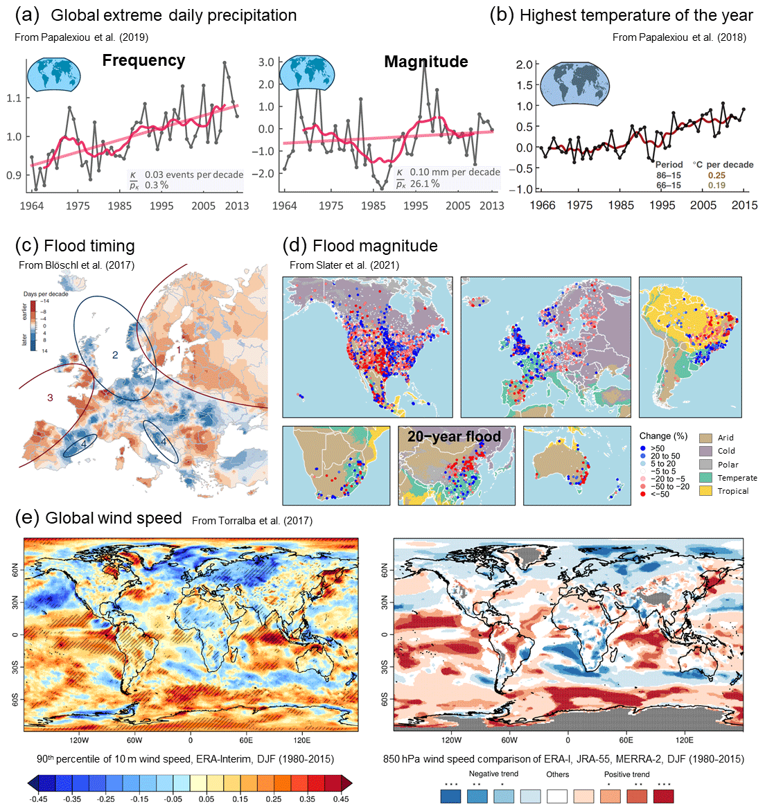
Figure 4Examples of trends in magnitude, frequency, and timing of hydroclimatic extremes. (a) Trends in extreme daily precipitation frequency (left plot – events) and magnitude (right plot – annual mean extreme daily precipitation anomaly; millimetres) over the globe (Papalexiou and Montanari, 2019). (b) Trend in the temperature anomaly of the highest temperature of the year (degrees Celsius) over the globe (baseline period – 1970–1989); the red line indicates 5-year moving average (Papalexiou et al., 2018). (c) Trends in flood timing across Europe in days per decade, 1960–2010 (Blöschl et al., 2017). (d) Trends in the magnitude of 20-year river floods, 1970s–present (Slater et al., 2021). (e) Global trends in wind speed. The left map shows the linear trend in metres per second per decade of ERA-Interim 90th percentile of 10 m wind speed for December–February (DJF; significant trends hatched). The right map shows the 850 hPa wind speed trends produced by ERA-I, JRA-55 and MERRA-2, where blues (reds) indicate the level of agreement between reanalyses about negative (positive) trends (Torralba et al., 2017).
POT methods are widely used to evaluate changes in the frequency of hydroclimatic events. These methods require selection of a reference threshold (a magnitude) and a period (e.g. 1 week) to decluster independent events. This is a common challenge for most hydroclimatic extremes (Fig. 3). For floods, many studies apply a somewhat arbitrary streamflow threshold that is, on average, exceeded twice per year (e.g. Hodgkins et al., 2019; Slater and Villarini, 2017a). In practice, alternative thresholds may be equally valid, such as the number of days when water levels exceed official flood thresholds (Slater and Villarini, 2016). However, setting a lower threshold means that events are less likely to be independent and/or of practical significance. Clusters of consecutive events are, thus, further declustered by specifying a period between events. For instance, Wi et al. (2016) separated extreme rainfall events by an interval of 7 d but other requirements have been proposed to ensure independence. Lang et al. (1999, p. 105) highlight that, in 1976, the U.S. Water Resources Council imposed a separation between flood events of “at least as many days as five plus the natural logarithm of square miles of basin area”, including a drop between consecutive peaks “below 75 % of the lowest of the two flood events”. The time between independent events depends on the catchment size, as a longer duration is expected in larger catchments because of the slower draw down of hydrograph limbs. In practice, such thresholds are far too short to adequately distinguish truly independent events, given the timescales of hydroclimatic variability which are often greater than a year. Similar concerns apply when isolating successive drought events (Bell et al., 2013; Thomas et al., 2014; Parry et al., 2016). Metrics for the identification of drought termination and, subsequently, drought independence include storage deficit methods that quantify the volume of water in relation to normal water storage conditions (Thomas et al., 2014) and, more generally, the return from maximum negative anomalies to above-average conditions (Parry et al., 2016). Hence, specification of the threshold and declustering technique make POT approaches more complicated to implement than block maxima approaches, where only one extreme per block (unit of time) is selected. More flexible selection of extremes and a larger sample size of frequency-based (i.e. POT) approaches may be preferred when record length is a limiting factor, whereas simpler magnitude-based (i.e. block maxima) approaches may be preferred when longer records are available.
More severe hydroclimatic extremes (such as 1 in 10-, 1 in 20-, 1 in 50-, 1 in 100-, or 1 in 200-year events) are typically evaluated using return periods (or expected waiting time). Alternatively, annual exceedance probabilities (AEPs) define the probability that a threshold will be exceeded in a given year. Other metrics have been proposed for engineering design. Reviews by Salas et al. (2018) and François et al. (2019) highlight ongoing disagreements about the utility of nonstationary methods for the design of engineering structures. As the uncertainties of nonstationary model structures may exceed that of stationary models (Serinaldi and Kilsby, 2015), specific strategies are required to manage the consequences of those uncertainties (François et al., 2019). There are, thus, ongoing debates about which concepts and methods are most appropriate for estimation of extremes, such as the return period, risk, reliability or equivalent reliability (ER), design life level (DLL) or average design life level (ADLL), and expected number of exceedances (ENE; e.g. Read and Vogel, 2015; Rootzén and Katz, 2013; Yan et al., 2017; Salas and Obeysekera, 2014). For instance, return period metrics may exhibit limitations in the case of time-correlated hydroclimatological extremes, so alternatives such as the equivalent return period (ERP; i.e. “the period that would lead to the same probability of failure pertaining to a given return period T in the framework of classical statistics, independent case”; Volpi et al., 2015) may be preferred.
It is not just individual characteristics of weather and water extremes that can change over time but also the interdependence between different characteristics, such as frequency, magnitude, and volume. Myhre et al. (2019) highlight that, in a warming climate, increases in extreme rainfall are likely to be driven by shifts in both the intensity and frequency of events, but increases in the frequency are most important. Brunner et al. (2019) assessed future changes in flood peak volume dependencies and found that the interdependence between variables may change more strongly than the individual variables themselves. This interdependency also applies to other variable pairs jointly of interest, such as drought duration and deficit or precipitation intensity and duration. Recognizing the interdependence between magnitude and frequency, many studies employ intensity–duration–frequency (IDF) metrics, which describe both the magnitude and frequency at once. It has recently been shown that generalized extreme value (GEV) distribution parameters scale robustly with event duration at the global scale (R2>0.88); hence, a universal IDF formula can be applied to estimate rainfall intensity for a continuous range of durations, including at the subdaily scale (Courty et al., 2019). There is growing interest in the nonstationarity of IDF curves (Cheng and AghaKouchak, 2014; Ganguli and Coulibaly, 2017) and the implications of this nonstationarity for compound hydroclimatic extremes globally (AghaKouchak et al., 2020).
2.3 Timing
Nonstationarity in the timing and seasonality of weather and water extremes has been examined far less than trends in magnitude and frequency (see examples in Table 1). Timing and seasonality provide information that is relevant for the management of water resources and analysis of underlying drivers of change. For instance, the start of field operations for farming may be estimated as the day of the year when “the sum of average temperature from 1 January exceeds 200 ∘C” (e.g. Rivington et al., 2013; Harding et al., 2015). Similarly, the start of the growing season may be measured as the first of 5 consecutive days with average temperature exceeding 5 ∘C (Rivington et al., 2013). Changes in these indicators of hydroclimatic extremes may have substantial impacts (e.g. crop yields). Additionally, changes in timing and seasonality can also affect the impacts of extreme events. For example, the risk from compound tropical cyclones and heatwaves is sensitive to the seasonal cycles in tropical cyclone probability (which peaks in late summer) and extreme heat (midsummer). A greater frequency of tropical cyclones earlier in summer, or more extreme heat late in summer, would increase the risk of compounding and attendant impacts (Matthews et al., 2019).
Changes in the timing of seasonal streamflow are typically assessed using the centre of volume (CV) date (Court, 1962) or mean date of flood occurrence (mean flood day – MFD). For example, Hodgkins and Dudley (2006) assessed changes in flood timing over the conterminous USA from 1913–2002 using the winter–spring CV dates. They found that a third of stations north of 44∘ had significantly earlier flows, likely related to changes in winter and spring air temperatures affecting winter snowpack. The MFD has been used to assess changes in streamflow timing in specific countries such as Wales (Macdonald et al., 2010) and Spain (Mediero et al., 2014). Probabilistic methods for identifying flood seasonality and their trends (Cunderlik et al., 2004) have been applied in Canada (Cunderlik and Ouarda, 2009) and the northeastern United States (Collins, 2019). In Europe, an analysis of 4262 streamflow stations in 38 countries used the date of occurrence of the highest annual peak flow to assess changes in flood timing (Blöschl et al., 2017). This showed significant changes in the seasonal timing of floods at the regional scale. In northeastern Europe, 81 % of stations had shifted towards earlier floods (by 8 d per 50 years), in western Europe, 50 % of stations had shifted towards earlier floods (by 15 d per 50 years), and around the North Sea, 50 % of the stations had shifted towards later floods (by 8 d per 50 years), as seen in Fig. 4c (Blöschl et al., 2017). Wasko et al. (2020b) evaluated global shifts in the timing of streamflow based on the local water year and found that shifts in the timing of annual floods were 3 times greater than shifts in mean streamflow. Furthermore, the drivers of streamflow timing depend on the magnitude of the event; less extreme events tend to correspond with soil moisture timing, while more extreme events depend more on rainfall timing (Wasko et al., 2020a).
Nonstationarity in the timing of extreme precipitation has also been used to better understand the causal factors of extremes. Gu et al. (2017) examined shifts in the seasonality and spatial distribution of extreme rainfall over 728 stations in China and found that alterations in rainfall seasonality were likely being driven by changes in the pathways of seasonal vapour flux and tropical cyclones. Others have examined shifts in the seasonality of future large-scale global precipitation and temperature extremes from model projections such as the Climate Model Intercomparison Project (CMIP; e.g. Zhan et al., 2020) (see Sect. 7.2 for a discussion of the projections). For instance, Marelle et al. (2018) investigated changes in the seasonal timing of extreme daily precipitation using CMIP5 models for RCP8.5 (high future emissions scenario) and found that, by the end of the 21st century, extreme precipitation could shift from summer/early fall toward fall/winter, especially in northern Europe and northeastern America. Brönnimann et al. (2018) employed a large ensemble of bias-corrected climate model simulations to understand changes in Alpine precipitation and found the annual maximum 1 d precipitation events (Rx1day) became more frequent in early summer and less frequent in late summer, due to summer drying.
3.1 Spurious nonstationarities: the issue of data quality
Confidence in nonstationarity detection, attribution, and prediction rests on confidence in the homogeneity and quality of input data – including the primary hydrometeorological series from individual observations, accompanying metadata, and qualitative information. Data quality issues tend to be particularly prevalent with measurement of extremes. Hydroclimatologists increasingly need to be aware of data quality issues associated with the homogeneity of remotely sensed data and their derivatives. For example, inaccuracies may arise from orbital drift (Weber and Wunderle, 2019), inference of precipitation from vegetation in data-sparse regions (Xu et al., 2015), or changing land surface reflectance such as snow cover over mountainous regions (Karaseva et al., 2012). Some of the most common sources of data errors and biases that reduce homogeneity or cause nonstationarity in ground-based information over timescales of years to decades are site or instrument changes, biases and drift in field procedures (time of sample and preferred values), unstable rating curves and channel cross sections, changes in network density/cover, post-processing, and archiving (unit changes; Wilby et al., 2017). For example, the England and Wales precipitation series is a specific example of spurious nonstationarity (a long-term trend towards wetter winters) arising from a combination of climate drivers (cold winters with more snowfall in the early 19th century) with non-standard rain gauges before the mid-1860s and snowfall undercatch, giving an apparent increase in winter precipitation (Fig. 5a; Murphy et al., 2020b). Gridded products and reanalysis data are also not immune from such data quality issues and are further affected by time–space variations in raw data inputs and version updates (Sterl, 2004; Ferguson and Villarini, 2014).
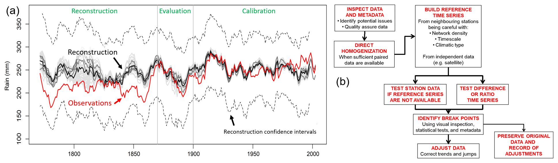
Figure 5Homogeneity of observational records. (a) An example of spurious nonstationarity in mean observed (red line) winter precipitation for England and Wales due to inhomogeneous records. The ensemble median and individual reconstructions (black and grey lines) do not exhibit nonstationarity (from Murphy et al., 2020b). (b) An approach to data homogenization for monthly to annual climate records (adapted from Aguilar et al., 2003).
Detecting spurious nonstationarities within raw data should be one of the first steps when evaluating time series that have yet to be quality controlled. Approaches have been proposed for uncovering homogeneity issues (see Fig. 5b). Common techniques for assessing data quality range from visual inspection or expert judgement to formal statistical tests (e.g. Chow test, Buishand range test, Pettitt test, and standard normal homogeneity tests). For meteorological variables, relative homogeneity tests are possible where appropriate networks of observations are available (e.g. HOMER; Mestre et al., 2013). However, such techniques are often limited to evaluating changes in the mean rather than extremes (Peña-Angulo et al., 2020; Ribeiro et al., 2016; Yosef et al., 2019).
An important step towards detecting and attributing nonstationarity is providing better metadata about measurement practice and any changes in observational techniques, as well as guidance on basic quality assurance approaches and the procurement and servicing of data sets. Observations are the foundation for understanding hydroclimatic change. Unfortunately, data sets of essential variables (precipitation, evapotranspiration, discharge, etc.) are typically disbursed across various global, regional, and national archives containing different variables and timescales in varied formats. For streamflow records, changes in the rating quality are rarely noted. Large, multi-country databases, such as the Global Runoff Data Centre (GRDC; https://portal.grdc.bafg.de/, last access: 6 July 2021), are vital for providing an overview of nonstationarities at continental and global scales but do not provide information on streamflow data quality. Accordingly, there are limitations on what can be said in global studies when compared with local knowledge. There is recognition of the need to create integrated data sets of observed variables for understanding and detecting change (e.g. Thorne et al., 2017). The CAMELS (catchment attributes and meteorology for large sample studies) initiative is an excellent start in hydrology, as these resources provide large integrated hydrologic data sets for regions of the world. CAMELS data sets already exist for the USA (Addor et al., 2017), UK (Coxon et al., 2020), Australia (Fowler et al., 2021b), Brazil (Chagas et al., 2020), and Chile (Alvarez-Garreton et al., 2018).
3.2 Record length and completeness
The observed record length required for assessments of nonstationarity depends on the type of process under consideration, the aims of analysis, properties of the underlying data, as well as the timescales of the sources of nonstationarity (drivers of change). For instance, Atlantic sea surface temperatures (SSTs) vary over periods longer than 50 years (McCarthy et al., 2015; Sutton and Dong, 2012) and affect concurrent precipitation and temperature patterns. The North Atlantic was particularly cold during the middle of the climate normal period (1961–1990) due to the Atlantic Multidecadal Oscillation or great saline anomaly (Dickson et al., 1988). Hence, even 50 years of data are insufficient to robustly detect true nonstationarities because the start and end dates of records may substantially affect the sign (direction) and magnitude of trends (Harrigan et al., 2018), especially in records that exhibit multi-decadal periodicity. Hundreds of years are required to adequately identify certain stationary models (Thyer et al., 2006), let alone nonstationary models. Additionally, highly variable time series require a larger percentage change in the mean of the data to identify a statistically significant change compared with less variable time series (e.g. Chiew and McMahon, 1993). In places where series have low signal-to-noise ratios, the time required to detect plausible trends (e.g. in precipitation, evapotranspiration, and discharge extremes) can, thus, be centuries long (e.g. Ziegler et al., 2005; Wilby, 2006). In some cases, faster detection may be possible using seasonal, rather than annual, time series (e.g. Ziegler et al., 2005).
The mismatch between the temporal scales of drivers of climate variability versus the availability and quality of observations can also result in misleading conclusions. For example, numerous studies have reported decreasing precipitation in Mediterranean regions since the 1960s (Longobardi and Villani, 2010; Gudmundsson and Seneviratne, 2016), with some attributing this decline and corresponding increase in drought frequency to anthropogenic forcing in the Mediterranean basin (e.g. Barkhordarian et al., 2013; Gudmundsson and Seneviratne, 2016; Hoerling et al., 2012). However, when viewed in the context of rescued and quality assured data beginning in the mid-19th century, these recent trends in precipitation are within the range of longer-term variability (Vicente-Serrano et al., 2019). Without sufficient record length, false attribution statements may arise with potentially significant management implications.
The challenges posed by the lack of available long-term observations have prompted some to leverage advances in data rescue and historical climatology to extend discharge series back in time (e.g. O'Connor et al., 2020; Smith et al., 2017; Bonnet et al., 2020). Palaeo-hydroclimatic reconstructions are also employed to extend data back in time and provide greater insight into current conditions. For example, warm and cool season rainfall was reconstructed in Australia to investigate the recent observed trend magnitude in the context of palaeoclimatic variability (Freund et al., 2017). Hydroclimatic reconstructions of the last 500 years have considerable potential to place recent observations into a long-term context that is not achievable from short observation-based record lengths alone. Although such data sets lengthen the period available for analysis and better reflect ranges of variability in extremes such as drought (Murphy et al., 2020a), they are subject to limitations from changes in measurement practice, decreasing density of observations in early records, and a lack of consideration of issues such as changes in land cover and shifts in channel capacity (Slater et al., 2015).
In many regions, temporal and spatial data sparsity is likely to remain a key issue, hindering robust detection, attribution, and prediction of water and climate nonstationarities. Therefore, different trend detection and attribution methods should be considered (e.g. using lower quantiles and peak over threshold methods; see Sect. 4), while implementing holistic “multiple working hypotheses” approaches (Chamberlin, 1890; Harrigan et al., 2014) to avoid overlooking potential drivers of change. Finally, gaps in extreme hydroclimatic time series may also affect the detection rate of significant trends. Detection rates are lower in records that have larger gaps and shorter length than those with less change (lower regression slopes) and fewer gaps and/or when the data gaps are located towards the beginning or end of a time series (Slater and Villarini, 2017a).
Detection of nonstationarity in hydroclimatological extremes requires a sound examination of the data before applying any statistical tests which broadly seek to detect the following two types of nonstationarity (see Fig. 1b): monotonic change (trends) and step changes (change points). Such changes can be considered as symptoms of nonstationarity if they represent a significant departure from normality within a long-term record. Nonstationarity may be detected either in individual time series (point-based analysis) or in larger ensembles of stations (spatially coherent trends; Hall et al., 2014). Here, we provide an overview of existing methods employed in the fields of weather and water extremes. For a description of change detection methods in hydrology, we refer the reader to Helsel et al. (2020) and, for floods, to Villarini et al. (2018). For an overview of methods and challenges in the detection and attribution of climate extremes, see Easterling et al. (2016).
4.1 Regression-based methods for detection of incremental change
The detection of trends in hydroclimatic time series generally employs the following two key approaches: detection of trends in magnitude (e.g. quantiles or block maxima, such as the annual maxima, AMAX) or frequency-based methods (e.g. use of point process modelling frameworks to model the peaks over threshold (POT) series, also referred to as partial-duration series (PDS; e.g. Coles, 2001; Salas et al., 2018).
The non-parametric Mann–Kendall (MK) test (Mann, 1945; Kendall, 1975) is a distribution-free test frequently employed to detect monotonic trends in time series without assuming a linear trend. Instead, MK simply evaluates whether the central tendency or median of the distribution changes monotonically over time (see Helsel et al., 2020). The test statistic, Kendall's τ, is a rank correlation coefficient which ranges from −1 to +1. For instance, Westra et al. (2013) evaluated trends in annual maximum daily precipitation at 8326 precipitation stations with at least 30 years of records and found increases at approximately two-thirds of these stations. A modified version of the MK test can also be applied to autocorrelated data (Hamed, 2009a, b). The Theil–Sen slope estimator (Sen, 1968; Theil, 1992; Hipel and McLeod, 1994) has often been used alongside MK (e.g. Hannaford et al., 2021) to estimate the magnitude of the trend over time (as the median slope of all paired values in the record). Different versions of the MK test exist to detect seasonal and regionally coherent trends over time (see Helsel et al., 2020, for details and examples).
Other studies also apply ordinary least square (OLS) linear regression to estimate trends in precipitation (e.g. Fig. 4a; Papalexiou and Montanari, 2019), temperature (e.g. Papalexiou et al., 2018), and flood flows (e.g. Hecht and Vogel, 2020). Practical advantages for using OLS methods include the ease of use and expression of uncertainty, graphical communication, and usability for providing decision-relevant information (e.g. Hecht and Vogel, 2020). In cases where the assumptions of OLS are not met (such as linearity, independence, normality, and equal variance of the residuals), non-parametric alternatives such as the Theil–Sen slope estimator or quantile regression (QR) may be used (both trend lines can be plotted). Instead of estimating the conditional mean of the response variable, QR considers different conditional quantiles (including the median) of a distribution. QR has been used for precipitation trends (e.g. Tan and Shao, 2017), air temperature (e.g. Barbosa et al., 2011), surface wind speed (e.g. Gilliland and Keim, 2018), and flood trends (e.g. Villarini and Slater, 2018) and is also regularly employed to investigate scaling properties between hydroclimatological variables (see Sect. 5.1; e.g. Wasko and Sharma, 2014).
When the empirical distribution of hydroclimatic extremes is known, many prefer to select an appropriate distribution and evaluate how the distribution parameters vary as a function of covariates such as time (e.g. Katz, 2013). For example, the nonstationary generalized extreme value (GEV) or Gumbel (GU) distributions are widely used to detect trends in annual or seasonal maxima such as floods (e.g. Prosdocimi et al., 2015), precipitation (e.g. Gao et al., 2016), and wind (e.g. Hundecha et al., 2008), while the Poisson (PO; e.g. Neri et al., 2019) or negative binomial (NBO; e.g. Khouakhi et al., 2019) distributions are preferred for discrete data (e.g. counts of days over thresholds). These distributions can be fitted to the data either with constant parameters (stationary case) or with the parameters expressed as a function of time (nonstationary case; Katz, 2013).
In the nonstationary case, a time or climate covariate can be employed to detect changes in the parameters of the distribution, as illustrated in Fig. 6. The advantage of employing climate covariates is that climate model predictions or projections can then be employed as covariates to estimate future change (as discussed in Sect. 7.3; e.g. Du et al., 2015). Criteria for model selection, such as the Akaike information criterion (AIC) or Schwarz Bayesian criterion (SBC; also known as the Bayesian information criterion – BIC) can then be used to determine whether the stationary or nonstationary model is the better fit (e.g. Fig. 6a). The AIC and BIC assess the trade-off between goodness of fit and model complexity, so the improvement in the goodness of fit must be sufficient to overcome the complexity penalty. Small differences in AIC are not always meaningful, such that several models may be equally acceptable (e.g. Wagenmakers and Farrell, 2004). In cases where the nonstationary model performs significantly better than a stationary model (in terms of goodness of fit and uncertainty), then the time series may be considered as nonstationary, pending sufficient record length (see Sect. 3.2).
Increasingly, distributional regression modelling frameworks, such as vector generalized linear and additive models (VGLM and VGAM, respectively) or generalized additive models for location, scale, and shape (GAMLSS), are being chosen for their flexibility in evaluating the nonstationarity of hydroclimatic extremes (e.g. Serinaldi and Kilsby, 2015). These frameworks are a generalization of generalized linear models (GLMs) that allow a broader range of distributions and different relationships between parameters and explanatory variables (linear, nonlinear, or smooth nonparametric). GAMLSS models, for instance, can have up to four parameters, i.e. μ, σ, ν, and τ, which allow for the modelling of the location (mean, median, and mode), scale (spread in terms of the standard deviation and coefficient of variation) and shape (skewness and kurtosis) of a distribution. An example of nonstationarity detection is shown in Fig. 6. Here, two nonstationary (with time-varying parameters) and two stationary (constant parameters) models are fitted using both the Gamma and Weibull distributions to observed time series of instantaneous (15 min) peak maxima (Fig. 6a). In the nonstationary case, the (μ and σ) model parameters both depend linearly on the time covariate (in years). A logarithmic link function is employed to ensure the distribution parameters remain positive. The goodness of fit of both stationary and nonstationary models is assessed using SBC (Fig. 6a). A detrended quantile–quantile (worm) plot showing the residuals for different ranges of the explanatory variable(s) can also be used to diagnose model fit (Fig. 6b). The model fit is satisfactory if the worm is relatively flat and if data points lie within the confidence intervals. In the case of the River Ouse, we find the nonstationary Gamma model is the best-fitting model. However, the Gamma and Weibull nonstationary model fits are fairly similar (Fig. 6a), and if the worm plots indicate a similar goodness of fit, it may well be that both are acceptable, but the Gamma nonstationary model is simply slightly better. Here, both the μ and σ parameters are increasing over time (Fig. 6c, d). The 50-year flood (specific discharge) increased from 0.123 m3/s/km2 in 1900 to 0.183 m3/s/km2 in 2018 (Fig. 6f).
GAMLSS methods have been applied for different hydroclimatic extremes. For example, Bazrafshan and Hejabi (2018) developed a nonstationary reconnaissance drought index (NRDI) to assess drought nonstationarity in Iran and found large differences between the NRDI and a traditional RDI (reconnaissance drought index) for time frames longer than 6 months. Sun et al. (2020b) also evaluated changes in a nonstationary standardized runoff index (NSRI) using GAMLSS over the Heihe River basin in China. An evaluation of global changes in 20-year river floods since the 1970s found a majority of increases in temperate climates but decreases in cold, polar, arid, and tropical climates (Fig. 4d; Slater et al., 2021). Importantly, the covariate in a GAMLSS nonstationary model is often time (e.g. Villarini et al., 2009a; Serinaldi and Kilsby, 2015) but may also include other physical drivers such as climate modes (e.g. Villarini and Serinaldi, 2012), urban or agricultural land cover (e.g. Villarini et al., 2009b; Slater and Villarini, 2017b), or other hydroclimatic variables such as dew point temperature (e.g. Lee et al., 2020).
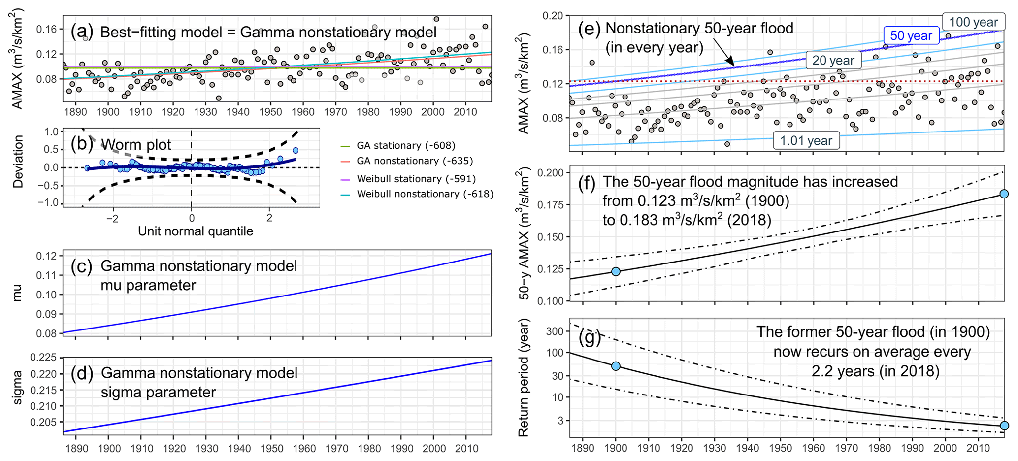
Figure 6Example workflow for detecting trends in the magnitude and return period of extremes using distributional regression (GAMLSS). The example shows a considerable increase in flood magnitude and frequency in the River Ouse in Skelton, UK, over 130 years. (a) In total, two nonstationary and two stationary models are fitted to the time series of 15 min peak maxima (black circles – specific discharge in cubic metres per second per square kilometre); colour lines indicate the 50 % probability (centile) for each model. The best-fitting model is the nonstationary Gamma model (lowest Schwarz Bayesian criterion, indicated in parentheses). (b) The worm plot indicates a satisfactory model fit (dashed lines indicate 95 % confidence interval). (c) Time series of the μ parameter for the nonstationary Gamma model. (d) Time series of the σ parameter (note that the mean of the distribution is equal to μ, and the variance is equal to σ2μ2). (e) Centile curves for the best-fitting nonstationary model are shown for the 1st, 50th, 80th, and 90th centiles (from bottom to top), 95th (20-year flood), 98th (50-year flood), and 99th (100-year flood). The dotted horizontal red line indicates the value of the 50-year flood in 1900. (f) The 50-year flood estimated every year from the nonstationary model increases over time. Confidence intervals given by dashed lines (5th and 95th). Blue circles indicate the estimated 50-year flood in 1900 and 2018. (g) The return period of the 50-year flood estimated in 1900 (with associated confidence intervals in 1900) is then estimated for every year using time-varying μ and σ parameters. Blue circles indicate the estimated return period in 1900 (50 years) and 2018.
Finally, there is growing interest in using interpretable machine learning methods for detection of nonstationarities in weather and water extremes. For example, Prophet (Taylor and Letham, 2018) is a decomposable time series forecasting model, similar to generalized additive models (GAMs; Hastie and Tibshirani, 1987), which is increasingly popular for hydroclimatological time series modelling. For example, Papacharalampous and Tyralis (2020) used the model for forecasting mean annual discharge 1 year ahead, and Aguilera et al. (2019) used the approach for groundwater-level forecasting. Prophet decomposes the time series into a trend component and a seasonal or periodic component, such as annual or daily cycles. The trend component is a piecewise linear growth model, meaning that, for each partition (piece) of the time series (separated by the change points), the model fits a unique trend (varying the trend over time), and the periodic effects are modelled as a Fourier series. This approach allows users to determine the locations in time when there are significant changes.
4.2 Pooled methods for detecting changes in extremes
As noted above, trend detection of hydroclimatic extremes is problematic when there is uncertainty arising from short record lengths or small samples. Extreme events such as the annual maximum, or 1 in n (50 or 100)-year events, tend to be highly variable and require lengthy time series to ensure robust detection of significant nonstationarities. In cases where the sample size of observed records is insufficient, alternative methods have been proposed, ranging from pooled sampling to scaling approaches.
Various pooled methods can be used to address the issue of limited sample size over large spatial scales. One pooled approach is to extract the single largest event over an n-year period from multiple independent gauge-based records, effectively substituting space (large spatial sample across many gauges) for time (long temporal sample at individual gauges). In other words, by pooling the data from multiple records or data sets, the data sample is increased for greater statistical robustness. For instance, Berghuijs et al. (2017) assessed changes in 30-year floods across multiple continents by noting the date of occurrence of the single largest daily streamflow at individual gauges and by evaluating the fraction of catchments experiencing their maximum flood at different points in time. This approach revealed temporal clustering of extreme flood occurrence at regional scales, i.e. flood-rich and flood-poor periods likely associated with hydroclimate variability. Max stable models (Coles, 2001) are another method of pooling data directly. The approach simulates spatial fields with observations from various point locations to increase the precision of statistical inference (e.g. Westra and Sisson, 2011).
Most statistical tests used to detect nonstationarity suffer from a substantial loss of power when applied to shorter time series (Yue et al., 2002b; Vogel et al., 2013; Prosdocimi et al., 2014, 2019). Pooled frequency analysis may improve the estimation of events associated with long return periods in rainfall IDF curves at sites where historical rainfall records are short or ungauged by compiling data from many rainfall records in a region (Requena et al., 2019). The areal model applied in Prosdocimi et al. (2019) serves a similar function, pooling regionally similar streamflow gauging stations to enhance shared trend signals. This approach can make clear the presence of trends that might otherwise remain obscured at individual sites due to short record length.
A different pooling approach for the detection of trends in extremes is the UNSEEN (UNprecedented Simulated Extremes using ENsembles) approach (e.g. Van den Brink et al., 2005; Thompson et al., 2017). UNSEEN pools members of seasonal predictions or large ensemble climate models (e.g. Deser et al., 2020), using the members as multiple realizations of a plausible alternate reality. In this way, historical sample sizes can be vastly increased to provide greater statistical confidence in extreme estimates. The method was further developed through an UNSEEN trends approach that enables detection of nonstationary extremes (e.g. precipitation) such as 100-year events from short (e.g. 30 year) climate model records (Kelder et al., 2020). The UNSEEN trends approach has the potential to detect nonstationarities in a range of climate extremes and can be applied to century-long seasonal hindcasts (e.g. Weisheimer et al., 2017, 2020). Furthermore, pooled members from dynamically downscaled climate model large ensembles have been used to estimate precipitation extremes and their nonstationarity in the past (Kirchmeier-Young and Zhang, 2020; Poschlod et al., 2021) and to estimate the likelihood of historic droughts under present-day greenhouse gases (GHGs; Cowan et al., 2020). However, there are some caveats. The reliability of UNSEEN trends rests on the independence, stability, and fidelity of underlying model members, as well as on the physical plausibility of the hazard-generating mechanisms in the model world.
If any of these pooled approaches is limited to a short period (e.g. half a century), however, it may not necessarily overcome all the challenges of record length. For instance, if a region is influenced by climate variability (e.g. positive Atlantic Multidecadal Oscillation, AMO, phase), increasing the sample size will not overcome the lack of data from other climate phases; the data still only originate from one of many possible states, and it is not possible to definitively conclude nonstationarity in behaviour of extremes over longer time periods. Thus, caution must be employed; short-term pooled approaches may be useful for investigating recent weather and water extremes (e.g. recent land cover changes, temperature scaling, or present climate risk analysis) but are less useful for explaining long-term drivers (e.g. climate variability) where longer records would be required. This caveat is equally applicable to all methods limited to short time periods.
4.3 Weather generators and synthetic time series
Weather generators and synthetic time series are powerful tools for capturing nonstationarity for weather variables and, more recently, even for streamflow at the catchment level. Such approaches can be used to inform decision-making. For instance, Benoit et al. (2018) developed a synthetic simulation approach for different types of rainfall, such as stratiform winter rainfall, spring rain showers, and heavy summer convective rainfall, based on their space–time–intensity structure. The rain types can be conditioned on different meteorological covariates (such as pressure, wind, temperature, or humidity; Benoit et al., 2020). The authors then applied this approach under a RCP8.5 (high) emissions scenario. In hydrology, synthetic design hydrographs (SDHs) may be used to test the sensitivity of the peak, volume, and shape of a flood hydrograph to the flood-generating mechanism and catchment properties (e.g. Brunner et al., 2018; Yue et al., 2002a). For instance, Brunner and Gilleland (2020) developed an empirical, wavelet-based model for stochastic simulation of streamflow time series (made available within the R package of PRSim). They showed that the method was suitable for sites exhibiting nonstationarities and spatial dependence of streamflow extremes, and that it can be used for water management applications.
4.4 Change point analyses for detection of abrupt change
Abrupt changes in hydroclimatic extremes are often a sign that there has been significant human intervention, such as the construction of a dam or diversion, which may significantly affect a catchment's water balance. Change point (also known as step trend) tests can thus be used either to detect such a shift or to compare two different periods separated by a long gap (Helsel et al., 2020). Several change point tests are available. The nonparametric Pettitt test is one of the most widely applied, and it allows the user to determine the timing of the change point and its significance (Pettitt, 1979). The performance of the Pettitt test – and other similar approaches, including pruned exact linear time (PELT; Killick et al., 2012), binary segmentation (Scott and Knott, 1974), Bayesian analysis (Erdman and Emerson, 2008), wild binary segmentation (WBS; Fryzlewicz et al., 2014), nonparametric PELT (Haynes et al., 2017), and the Mann–Whitney test (Mann and Whitney, 1947) – for the estimation of abrupt changes in the mean, variance, or median of a time series was tested using both simulated and historical data with known change points (Ryberg et al., 2019). Although these methods offer potential benefits (such as the detection of multiple change points), the comparison found that the Pettitt test delivered the best combination of change point detection and minimization of false positive results. The parametric tests (PELT, binary segmentation, and Bayesian analysis) generally performed poorly at detecting known change points in peak streamflow, while the non-parametric tests (non-parametric PELT and Mann–Whitney) and the parametric WBS resulted in unacceptable false positive rates (Ryberg et al., 2019). The Mood test (Mood, 1954; Ross et al., 2011) for abrupt changes in scale was also evaluated in the same study but located only about 25 % of known change points in historical data (with a relatively low false positive rate) and approximately 29 % of change points in simulated data (with a relatively high false positive rate).
4.5 Circular statistics and methods for detection of shifts in timing
Circular statistics, a branch that focuses on directions, axes, or rotations, can show changes in the timing and seasonality of hydroclimatic extremes. Circular statistics have been applied to precipitation (e.g. Gu et al., 2017; Marelle et al., 2018; Brönnimann et al., 2018), snowpack (Hamlet et al., 2005; Mote et al., 2005), and streamflow (e.g. Villarini, 2016; Hall and Blöschl, 2018; Blöschl et al., 2017; Wasko et al., 2020b; Barnett et al., 2008). The null hypothesis of circular statistics, when applied to timing, is that data are evenly distributed (uniform) with no tendency to cluster. Different methods can be used to calculate the trend in timing, such as circular regression (Wasko et al., 2020a), measures of linear–circular association (Villarini, 2016), the Theil–Sen slope estimator (Blöschl et al., 2017), linear regression (Barnett et al., 2008), and linear regression after standardization on the local water year (Wasko et al., 2020b). In total, the following three seasonality types can also be detected: circular uniform (no preferential direction, indicating that an event has the same probability on any day of the year), reflective symmetric (unimodal), and asymmetric (multi-modal, e.g. locations with multiple generating processes, such as snowmelt and mesoscale convective systems in the case of flooding) (Villarini, 2016).
For precipitation, Gu et al. (2017) found a significant shift in the seasonality of extreme rainfall using circular statistics, which suggested that pathways of seasonal vapour flux and tropical cyclones were likely driving these changes. For flooding, an approach based on seasonality statistics was developed to evaluate changes in the dominant flood-generating processes across Europe. Berghuijs et al. (2019b) used the mean date of occurrence of three processes (extreme precipitation, soil moisture excess, and snowmelt) to estimate the relative importance of each process at 3777 European catchments with at least 20 years of flood peak timing data. They found that the relative importance of mechanisms had not changed significantly over 50 years. Similarly, Macdonald et al. (2010) used the mean day of the flood (MDF) to assess changes in flood timing over Wales. They used a directional statistic, computed by counting the number of days from 31 May (the date is chosen to provide a more normal distribution of British floods over the year) until the event and then converting the day of flood occurrence to an angular value ((θ); a direction). Shifts in the timing of extreme weather events can also be assessed by comparing the number of events per season between present and future climate simulations. For example, Whan et al. (2020) show that July–September could experience an increase in the number of landfalling atmospheric rivers over Norway by the end of the century. They find that the seasonal differences are reduced in the far-future period, with an equal number of atmospheric river events in winter and summer, hence suggesting a seasonality shift.
The terms of mechanisms, agents, and drivers are often used in the context of hydroclimatic extremes and are sometimes used interchangeably or with different intents. Here, we distinguish between these terms as follows. The expressions of hydroclimatic agents or hydroclimatic mechanisms refer to the processes generating hydroclimatic extremes. Depending on the temporal and spatial scale, precipitation-generating agents might include local convection, synoptic weather patterns, or cyclones; flood-generating mechanisms might additionally include snowmelt or ice jam release. The expression of nonstationary drivers refers to longer-term processes which may cause significant shifts in the underlying distributions of hydroclimatic extremes via climate or land cover change. Here we focus more on the drivers of nonstationarity than the extreme-generating mechanisms and agents. It is important to note that other (non-process related) factors may also generate spurious nonstationarities (see Sect. 3.1).
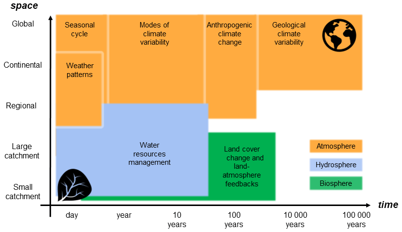
Among the different hydroclimatic extremes, it is widely recognized that temperature is easier to attribute than precipitation, floods, and storms. Dynamically driven extremes are harder to attribute because they typically have smaller signal-to-noise ratios and higher uncertainty (see, e.g., Trenberth et al., 2015). The drivers or sources of nonstationarity are predominantly artificial – i.e. human impacts such as land cover change, river regulation, and anthropogenic climate change. They may operate over a range of timescales, from the annual timescales of water management (abstraction and water transfers) and some abrupt land surface changes (e.g. urbanization or impacts of forest fires) to the (multi-)decadal timescales of climate change. In contrast, natural periodicities, such as the seasonal cycle, weather patterns, climate modes of variability, and geological climate variability, may not necessarily drive nonstationarity when considered over their full timescales. The geographical impact of climatic drivers (Sect. 5.1) is typically much broader than for land cover (Fig. 7); by contrast, land cover change is often long-lived but largely local (Sect. 5.2). Water management decisions (Sect. 5.3) may propagate far beyond the catchment to region, country, and beyond when teleconnection effects occur (Sect. 5.4). However, the effect of these nonstationary drivers and their interaction (such as the impacts of anthropogenic climate change on climate modes) is complex and not yet fully understood; the same drivers affect extremes in different ways, depending on the site-specific conditions over different spatial and temporal scales. Finally, the drivers of compound extremes are still an emerging area of research (Sect. 5.5).
5.1 Climate variability and change
Climate change is widely recognized as being one of the most important multi-decadal to millennial drivers of changes in hydroclimatic extremes. Potential impacts may be expressed primarily through the water cycle, as storminess and rainfall extremes are projected to increase with warming (Hartmann et al., 2013; Kharin et al., 2013; Held and Soden, 2006; Kossin, 2018). However, the association between warming and hydroclimatic extremes is not straightforward; there is not a one-to-one relationship between increases in temperature, precipitation, and floods (e.g. Wasko and Nathan, 2019; Wasko et al., 2019), and the effects of climate change operate over different temporal and spatial scales.
To understand how warming may affect intense rainfall and floods, studies have assessed the nature of scaling relationships between extremes. As air temperature warms, the intensity of extreme precipitation is expected to increase due to the enhanced water-vapour-holding capacity of warmer air, approximately following the Clausius–Clapeyron relation (C–C; 6 %–7 % per degree Celsius; e.g. Trenberth et al., 2003; Ali et al., 2018, and see Fowler et al., 2021a, for a recent summary of the research on short-duration rainfall extremes under climate change). Generally, peak rainfall intensities increase with both regional and global temperature. Some studies have shown that extreme precipitation is expected to become more intense and weaker rainfall less intense (Wasko and Sharma, 2015). However, further investigation is needed as there are contrasting results regarding the decline in light precipitation, so the compensation mechanism is still unclear (Markonis et al., 2019). Increases in precipitation extremes in response to warming are greater for convective precipitation (a super C–C rate) compared with stratiform precipitation (a normal C–C rate; Berg et al., 2013). Furthermore, it has been suggested that the transition from C–C scaling to super C–C scaling may occur at higher temperatures (approximately 20 ∘C) in regions with climatologically lower frequency of convective events (e.g. approximately 20 ∘C in South Korea vs. 12 ∘C in certain European regions; Park and Min, 2017). Other of the key questions is whether precipitation intensities are likely to increase proportionally over shorter timescales. Research suggests that temperature–rainfall scaling increases over hourly timescales (Lenderink and Van Meijgaard, 2008). For example, UK summer precipitation is estimated to increase by 30 %–40 % for short-duration extreme events (Kendon et al., 2014).
What does temperature scaling mean for floods and droughts? There is still little evidence that increases in heavy rainfall events at higher temperatures translate into similar increases in streamflow (Wasko and Sharma, 2017). Increased extreme rainfall does not necessarily lead to increased flooding (Blöschl et al., 2019). There are many other factors that affect flood response besides precipitation intensity, including the duration and extent of precipitation events, antecedent soil moisture conditions, catchment size, vegetation cover, and catchment imperviousness and roughness (Sharma et al., 2018). Studies have found that lower annual recurrence interval floods are more likely to be reduced due to drier antecedent soil moisture conditions, whereas higher annual recurrence interval floods are more likely to increase due to increases in extreme rainfall (Fig. 7 in Wasko and Nathan, 2019). In temperate climates of northwestern Europe, extreme precipitation is an important flood driver, while in the drier climates of southern Europe, both antecedent soil moisture and extreme precipitation matter (with a greater importance of soil moisture for smaller floods; Bertola et al., 2021). Increases in precipitation intensity are more likely to cause increases in streamflow in smaller catchments (Wasko and Sharma, 2017; Wasko and Nathan, 2019). Perhaps counter-intuitively, streamflow is likely to decrease in catchments that are experiencing significant reductions in the fraction of precipitation falling as snow (Berghuijs et al., 2014). In high-altitude, snowmelt-dominated regions such as the Hindu Kush Himalayan “water towers of Asia” (Immerzeel et al., 2020), where a large amount of water is stored as snow or ice, expected climate shifts could accelerate glacier and snowpack melting. This may, in turn, lead to more frequent glacial lake outburst floods, flash floods, and riverine floods, thus posing potential risks to the 240 million people in the region and the 1.9 billion people living downstream (Wester et al., 2019). Yet, it is important to note that, in many locations, the effects of climatic shifts may represent only a minor source of variability when compared with more direct anthropogenic influences such as reservoirs and land cover change (Lins, 2012).
The effects of climate change on wind are less understood than precipitation, temperature, or hydrological extremes. Although the intensity and location of future storm tracks depend on changing temperature gradients, the response is likely to be variable because those temperature gradients are expected to change in a non-uniform manner. For example, Harvey et al. (2014) found a consistent positive relationship between the change in temperature gradient and storm track intensity across CMIP5 models, but a highly variable storm track response (e.g. with strengthening over the UK yet weakening over the USA). This is explained by a weakening temperature gradient over the USA (due to Arctic amplification), and a strengthening gradient over the eastern Atlantic – likely explained by changes in ocean circulation (Woollings et al., 2012). Over large spatial scales, climate change also affects the characteristics (magnitude, frequency, and timing) of the synoptic-scale phenomena that generate hydroclimatic extremes, such as atmospheric rivers (ARs), tropical cyclones, and atmospheric circulation patterns (e.g. Hirschboeck, 1988; Schlef et al., 2019). For example, ARs play a major role in flood occurrence in many regions of the world (Lavers et al., 2011, 2012; Paltan et al., 2017), and thus, changes in their frequency and characteristics could alter the properties of future hydroclimatic extremes. In regions such as Norway, where rainfall extremes are primarily driven by ARs (Whan et al., 2020), changes in the phase of precipitation are leading to increasingly rainfall-dominated, rather than snowfall-dominated, regimes which may alter flood characteristics and water resource management. Where snow would otherwise be stored in the catchment, rainfall is likely to contribute more directly to runoff, leading to more severe AR-induced floods but less severe snowmelt-driven floods later in the season.
The effects of climate variability on hydroclimatic extremes are well recognized. Hazard-rich and hazard-poor periods in the historical record tend to be driven by the spatial and temporal periodicities of multiple, sometimes overlapping, climate modes. For instance, during a positive phase of the North Atlantic Oscillation (NAO), the jet stream tends to shift northwards, generating a greater frequency of heavy rain events over the British and Irish islands (Hannaford and Marsh, 2008). The NAO, together with the Scandinavian pattern (SCA), is also the main driver of European windstorm variability (Walz et al., 2018). Understanding the exact mix of atmospheric influences driving flood-rich periods, such as the exceptionally flood-rich past 3 decades in Europe, requires ongoing work (Blöschl et al., 2020). El Niño–Southern Oscillation (ENSO) phases have different effects on flooding and droughts, depending on locality. In Central America, for instance, the west coast experiences increased likelihood of droughts during the El Niño phase of ENSO, while the east coast has increased flood risk (Cid-Serrano et al., 2015; Enfield and Mayer, 1997; Aguilar et al., 2005). Moreover, El Niño events have been observed to drive episodes of extreme heat in Southeast Asia (Thirumalai et al., 2017), whilst also increasing the lifetime and strength of tropical cyclones in the western North Pacific (Camargo and Sobel, 2005). Temperature extremes in northern Europe are associated with atmospheric blocking situations, both during winter cold spells (Sillmann et al., 2011) and summer heatwaves (Schaller et al., 2018). However, the interlinkage between climate variability and change is still not fully understood for atmospheric blocking and remains challenging to disentangle (e.g. Woollings and Blackburn, 2012; O’Reilly et al., 2019).
5.2 Land cover changes
Land cover modulates the response of local, regional, and remote regions to shifts in climate variability and change. Land is both a source and sink of greenhouse gases; expansion of areas under agriculture and forestry may alter hydroclimatic extremes through a combination of both biophysical effects (e.g. photosynthesis, respiration, drying, and greening) and greenhouse gas feedbacks (see Chapter 2 of IPCC, 2019).
The effect of urbanization on hydroclimatic extremes is perhaps one of the most well-documented land cover changes, but there are still many unknowns. Cities alter the local atmosphere through the urban heat island (UHI) effect which increases the mean annual surface air temperature within cities relative to surrounding rural areas. The magnitude and diurnal amplitude of the UHI effect varies between cities (Ward et al., 2016), lifting night temperatures more than daytime temperatures (Hausfather et al., 2013). For example, in Kuala Lumpur, Malaysia, hourly intensities of extreme rainfall have increased by ∼35 % in the last 30 years due to the UHI creating an unstable atmosphere (i.e. altering the local atmospheric vertical structure; Li et al., 2019). The effects of these local land surface changes are compounded by the thermodynamic and dynamical effects of climate change. Local changes in extreme temperature are driven over short or medium spatial and temporal scales by changes in the land surface such as the UHI effect and large-scale irrigation (e.g. Mahmood et al., 2014), but over multi-decadal timescales, they are principally caused by large-scale shifts in greenhouse gases modifying the global mean temperature.
Urbanization effects on flooding and drought are also widely acknowledged but not yet fully understood. Prosdocimi et al. (2015) evaluated the impacts of urban land cover in a paired-catchment study in the UK using both block maxima and POT approaches. They found a significant effect of urbanization on high flows in all seasons, with the strongest effect in summer. A recent analysis of 280 stream gauges in the United States found that annual maximum floods increase by 3.3 % on average for every 1 % increase in impervious land cover, using panel regression (e.g. Blum et al., 2020). Furthermore, the vertical structure of cities can alter precipitation and flood extremes. When Hurricane Harvey hit Houston, Texas, in August 2017, enhanced rainfall was produced by the storm system's drag induced by increased surface roughness (Zhang et al., 2018). Another recent study examined the effect of urbanization on long-term persistence in the streamflow records of 22 catchments in the northeastern United States using scaling exponents (Jovanovic et al., 2016). They found evidence that streamflow responds more quickly to rainfall in urbanized catchments than in less urbanized counterparts.
Increases in vegetation cover, termed “greening”, are occurring in many regions, both as a result of human afforestation and potentially through a fertilization effect caused by increases in global CO2 (expected to lead to greater water consumption; e.g. Ukkola et al., 2016). Nonlinear feedbacks between atmospheric and land surface processes can also lead to varying carbon uptake in vegetation (e.g. soil moisture may alter photosynthesis rates; Humphrey et al., 2021). Afforestation and deforestation affect both floods and droughts – sometimes in more ways than one. For example, afforestation can increase streamflow magnitude by ditching but can also reduce flood peaks by canopy interception, evapotranspiration, and drier antecedent conditions (e.g. Birkinshaw et al., 2014; Soulsby et al., 2017). The effects of changes in vegetated land are believed to be far more pronounced for low flows than high flows (e.g. Birkinshaw et al., 2014; Bathurst et al., 2020; Do et al., 2017; Vicente-Serrano et al., 2019), although there have been very few large-sample studies using observational records. To understand the influence of land cover changes on catchment hydrology, numerical modelling is often used to assess potential impacts and provide evidence for ambitious land cover changes related to policy before implementation. Some have employed theoretical land cover changes (e.g. Gao et al., 2018; Iacob et al., 2017); others used scenario-based land cover changes (e.g. Harrison et al., 2019). The response of hydroclimatic extremes to land cover change varies over both spatial and temporal scales. At the very fine scale, the hydraulic structure of the soil may change due to the reorganization of macro- and micro-pores associated with land management practices within a single parcel of land. At continental and multi-decadal scales, changes in the magnitude, intensity, and pathway of storms may lead to widespread changes in runoff. These effects may not be distinguishable over short periods in individual catchment data, so long-term monitoring is required to understand their impact on catchment hydrology over a range of spatial and temporal scales (Dadson et al., 2017).
Major land cover changes may also have remote teleconnection effects on hydroclimatic extremes. For instance, it has been shown that tropical deforestation alters precipitation patterns not only locally but also in the mid- and high latitudes. Deforestation of the Amazon and central Africa may reduce precipitation in the USA Midwest, while the deforestation of Southeast Asia has been shown to affect China (Avissar and Werth, 2005). In northern India, Saeed et al. (2009) found that irrigation suppresses the development of monsoon-driving land–sea temperature gradients and, thereby, exerts a first-order control on precipitation in central India and the Bay of Bengal.
5.3 Water resources management and geomorphological change
With the growing demand for food and increased productivity following the mechanization of agriculture, large swathes of land have been subject to arterial and land drainage. Such installations can take various forms. Their impact on the hydrological response is poorly understood, but they may alter catchment morphology, soil, and groundwater hydrological response, depending on the extent of the catchment affected and the extent of works completed on river channels. The nature of hydrological nonstationarities associated with arterial and field drainage has been debated; some argue that changes should not be detectable in discharge as abrupt shifts, while others have identified change points in specific components of the hydrological regime (Harrigan et al., 2014). Numerous studies showed that arterial and field drainage can affect flood peaks (increasing magnitude and reducing time to peak; e.g. Wilcock and Wilcock, 1995; Bhattarai and O'Connor, 2004). Conversely, our understanding of the impacts of drainage on low flows and drought remains poor, as does our understanding of how other components of runoff response are affected due to inadequate monitoring of subsurface hydrological processes.
Changes in river channel morphology and conveyance capacity are also poorly understood drivers of changes in flooding. In the Mississippi River, for example, construction of wing dikes, navigational structures, and levees contributed significantly to increases in flood levels (Pinter et al., 2008). Decreases in river conveyance may significantly affect the frequency of overbank flooding and can be identified from trends in flood stages (Pinter et al., 2006) and from stream gauge transect data (James, 1991; Smelser and Schmidt, 1998). It is now possible to estimate the relative effect of hydrologic and geomorphic drivers of changing flood risk (Slater et al., 2015) and even to estimate the influence of tropical cyclones on conveyance and flood risk (Li et al., 2020).
Water management can also generate significant nonstationarities. Dam construction increased dramatically over the last century and is likely to continue apace in developing regions. Grill et al. (2015) highlighted that, on a global basis, 48 % of river volume was moderately to severely impacted by either flow regulation, river fragmentation (i.e. diminished connectivity within river systems), or both as a result of dam construction. The impacts on trends in river flow have been debated. Lorenzo-Lacruz et al. (2012) examined trends in Iberian river flows over the period 1945–2005, finding that river regulation by dams was more likely to affect the magnitude of trends rather the direction of change with important seasonal differences. Examining trends in floods at a global scale, Do et al. (2017) found that the presence of dams did not have a large impact on trend results in all catchments. Rather, catchment size and local context were deemed to be most important in determining response. Abstractions and discharges from watercourses can also drive nonstationarities; thus, an important task in the detection of climate or land cover impacts is to ensure that naturalized flow regimes are employed.
5.4 Land–atmosphere feedbacks
Nonstationarity can also arise when nonlinear dynamical systems exhibit multiple metastable states. Much debate has arisen in the literature surrounding the flawed diagnosis of nonstationarity in systems that have metastable states due to internal feedbacks. The difficulty is particularly acute when records are short and understanding of the system is poor. Examples of metastable states imposed by the climate system include the persistence of periods of high levels in Lake Victoria (Sutcliffe and Parks, 1999), now thought likely to be driven by the Indian Ocean Dipole (Schott et al., 2009). Important examples of land–atmosphere feedbacks internal to hydrological systems include the role of rainfall recycling in Amazon dieback (Wenzel et al., 2014). Feedbacks are also thought to have amplified climate variability in the Sahel and in the 20th century western USA dust bowl (Berg et al., 2016). More recently, the role of soil moisture storage in controlling land–surface feedbacks was highlighted through enhancement of heatwaves and associated severe drought conditions in central Europe (e.g. Seneviratne et al., 2010; Kornhuber et al., 2020). In Australia, both positive and negative correlations have been found between daily soil moisture and next-day rainfall, depending on spatial scale, location, and season (Holgate et al., 2019). Of key importance is the potential for human water use to affect the water balance in regions where hydrological systems are close to sensitive thresholds (Gleick and Palaniappan, 2010). These examples demonstrate that internal feedbacks in hydrological systems can amplify nonstationary drivers of change. Moreover, some of these feedbacks exhibit behaviour which suggests that they introduce tipping points in the Earth system; thus, this can also become a driver of nonstationarity (Lenton et al., 2008). Analyses which address the mechanisms behind such feedbacks will be required in order to account for their effects in the future.
Most of the time, there are many drivers affecting hydroclimatic extremes simultaneously across overlapping multiple temporal and spatial scales (Fig. 7). This makes it all the more challenging to discern their individual effects.
5.5 Compound drivers: difficulties in understanding nonstationarity in compound risk and consecutive disasters
Interest in compound hydrological extremes is growing rapidly, not least because these events can deliver particularly severe societal impacts (de Ruiter et al., 2019; Raymond et al., 2020a; Zscheischler et al., 2020). Although rarity and complexity pose challenges for their assessment, physical reasoning and empirical methods have highlighted that they can be sensitive to anthropogenic climate warming (AghaKouchak et al., 2020) and modes of climate variability (Hillier et al., 2020). It is also possible that novel compound hazards (such as enhanced wildfires in 2019 in California, caused by a combination of wind and low-humidity events) may emerge as the climate continues to change (Raymond et al., 2020a; Matthews et al., 2019), causing potentially devastating consequences for communities taken by surprise (Masys et al., 2016). With so much at stake, losses from novel hazards may be too substantial to learn from once they have emerged (Masys et al., 2016; Sornette and Ouillon, 2012). Instead, modelling and simulation can be used to explore extreme unseen events (Sect. 4.2) as well as resampling and stochastic weather generation techniques that provide a quantitative underpinning to storyline approaches (Woo, 2019; Shepherd et al., 2018; Matthews et al., 2019).
The role of spatial and temporal correlations in hydrological hazards like drought is important for probabilistic calculations of risk. For example, simultaneous crop failure in Russia, southwestern Australia, and southwestern China caused a major spike in grain prices in 2011–2012 (e.g. Gaupp et al., 2020). Crop production losses can be underestimated by a factor of three if spatially correlated risks are ignored, but losses can be reduced by international cooperation to pool risks (e.g. Gaupp et al., 2020). Coincident hydrological extremes at the global scale can be driven by climate modes such as ENSO, the Pacific Decadal Oscillation, and the Atlantic Multidecadal Oscillation (De Luca et al., 2020).
The term attribution implies an understanding of the causes or driving processes of change. In the climate sphere, it is often understood in a strict sense as quantifying the influence of humans on the climate or demonstrating that climate change is consistent with climate model predictions rather than alternative causal explanations. However, beyond climate science, the field of attribution is still relatively new. In hydroclimatology, the concept of attribution is used more broadly to disentangle the wide range of drivers of hydroclimatic extremes, which include climate variability, land cover change, and land–atmosphere feedbacks (Sect. 5). Attribution is typically preceded by exploratory data analysis (EDA) in order to understand the underlying data (Sect. 6.1). Attribution methods can then broadly be divided into empirical (Sect. 6.2) and simulation-based (Sect. 6.3) approaches. Empirical approaches use statistical techniques to relate the causes to detected changes in the observed record. Simulation-based approaches use model simulations to explain drivers of changes in climatic extremes. In both cases, attribution requires developing multiple working hypotheses based on a process-based understanding of potential drivers of change (Harrigan et al., 2014).
6.1 Exploratory data analysis (EDA)
Exploratory analyses play an essential role in understanding historical changes. Often, such analyses involve a visual exploration of the time series and of the statistical test results for many gauges to identify common patterns or outliers. At the most basic level, temporal trend lines (e.g. Fig. 6f) from multiple stations can be plotted on the same graph to identify any record that diverges from the coherence of the pooled analysis. Similarly, trend persistence plots may be created for multiple stations to identify suspect data where nonstationarities may be present. For example, Noone et al. (2016) computed the MK Z score over different time periods, starting with the full record, then shortening the start year by 1 year at time to a minimum length required for statistical robustness (such as 30 years). Plotting persistence lines for multiple stations allowed them to flag stations with possibly spurious nonstationarities. Wavelet power spectra can also be plotted for multiple stations to assess whether a common periodicity can be detected across multiple sites. For instance, Rust et al. (2019) used continuous wavelet transforms to identify multi-annual periodicities of the North Atlantic Oscillation in UK groundwater records.
6.2 Empirical attribution approaches
Statistical attribution of hydroclimatic nonstationarity is typically regression based. Statistical methods require less computational power than physical model-based approaches but cannot account for complex feedbacks between processes. Additionally, statistical approaches are unable to distinguish between correlation and causation, even when a predictor is physically plausible. The first step in attributing the drivers of a nonstationary process is to detect the presence of nonstationarity in the time series. This can be done by applying a trend plus significance test (Sect. 4.1) or by fitting a distributional regression model with constant parameters (stationary case), and then again with time-varying parameters (see Fig. 6a), and evaluating the superior description of the data. If the stationary model fit is better (e.g. lower AIC or SBC), then it is not recommended to proceed further. If the time-varying model is better, and if there are physically plausible reasons to suspect nonstationarity, then attribution may proceed. However, it is important to note that small differences in AIC and SBC are not always meaningful (Burnham and Anderson, 2004), and a visual assessment is generally recommended. If a time series is deemed nonstationary, regression can be used to determine potential drivers of change by introducing predictors that are representative of the drivers (e.g. changing land cover, climate, or reservoir indices). Regression model coefficients can be used to quantify the effect of covariates (e.g. Prosdocimi et al., 2015).
Panel regression techniques are increasingly popular because they can be used to leverage temporal and spatial variation to isolate a causal effect, which is separate from other drivers of change (Blum et al., 2020). These methods pool both dynamic (e.g. land cover) and static (e.g. physical catchment characteristics) data across time and space. They are able to identify generalized relationships between drivers and hydrologic response (i.e. reliable model coefficients) and are particularly powerful in regional and large sample analyses (Bassiouni et al., 2016; Steinschneider et al., 2013). Examples of recent applications of panel regression include estimating low-flow response to rainfall in ungauged basins (Bassiouni et al., 2016) and estimating the effects of urbanization on annual runoff coefficients (Steinschneider et al., 2013) and peak flows in the USA (Blum et al., 2020) and in Belgium (De Niel and Willems, 2019). Others have applied panel regression to analyse the effects of forest cover change and other socioeconomic factors on the frequency of large floods in developing regions (Ferreira and Ghimire, 2012) or to examine the effects of deforestation and agricultural development on streamflow in Brazil (Levy et al., 2018).
6.3 Simulation-based attribution of nonstationary extremes
Unlike statistical methods, where models are fitted to observations, climate model experiments are physically based; they solve series of mathematical equations representing various Earth system processes. The strength of these methods relies on their use of physics to accurately describe real-world feedbacks and recognize important physical limits; for example, the cap on extreme humid heat in the tropics linked to deep convection (Sherwood and Huber, 2010; Zhang and Fueglistaler, 2020). Here we provide a brief overview, but we point the reader to Hegerl et al. (2010) and IPCC (2013) for details.
In attribution studies, climate models can be run under different scenarios to identify the role of anthropogenic forcing in contributing to the likelihood of an observed extreme. For example, comparing the probability of an extreme event simulated by a model for the current climate (p1) with its probability in a modelled pre-industrial scenario (p0), indicates how much more likely () the event has become relative to a counter-factual world in which the pre-industrial climate persisted (see Fig. 8a, b). The probability ratio framework is also used to identify the “fraction of attributable risk” () – the portion of the event's probability that can be assigned to anthropogenic modification of the climate (Fischer and Knutti, 2015). Changes in event magnitude can also be examined using the same framework. Wang et al. (2018) applied such methods to the exceptional rainfall caused by Hurricane Harvey in 2017. The analysis indicated that, in a counter-factual environment of no trends in SSTs or tropospheric variables, the storm would have delivered almost 30 % less precipitation. Such methods, which blend climate change scenarios with numerical weather prediction models can also be used to assess how the characteristics of observed extremes may differ in counter-factual worlds (hotter or colder than present). Lackmann (2015) demonstrated this for Hurricane Sandy, noting that climate warming since pre-industrial levels caused a small northward shift and intensification of the storm's track; further intensification and northward displacement could be expected in a counterfactual climate even warmer than that observed in 2012. Statistical comparisons, such as the Anderson–Darling (AD; Fig. 8c) or Kolmogorov–Smirnov (KS) tests, can formally confirm any significant differences between historical observations and future simulated extremes. The AD test is often more powerful when comparing two distributions than the KS test (Engmann and Cousineau, 2011).
Other studies have compared observations and multi-model simulations of changes using an optimal fingerprinting technique, where observations are regressed onto the simulated responses to external forcing (fingerprint patterns). Analysis of the regression coefficients estimates and uncertainties (scaling factors) is used to detect fingerprints in the observations when the scaling factors are positive. For instance, Min et al. (2011) compared observed and simulated long-term variations in a probability-based index (PI) and attributed the intensification of extreme rainfall over much of the Northern Hemisphere land areas to human-induced climate change. The fingerprint method was also recently used to attribute global trends in mean and extreme streamflow to anthropogenic climate change (Gudmundsson et al., 2021).
Attribution often requires running large model ensemble experiments, which can be computationally expensive. The project of https://www.climateprediction.net/ (last access: 6 July 2021) was established to make use of thousands of home computers volunteered by individuals to enable ensemble runs of global or regional climate models. These many runs can be used to quantify internal ensemble variance and compare it to observed events. The project now runs regional large ensemble citizen science experiments called “weather@home”, which are used for probabilistic event attribution (Massey et al., 2015; Guillod et al., 2017). For example, this regional ensemble approach was used to demonstrate the human influence on climate in the 2014 southern England winter floods (Schaller et al., 2016) and the 2003 European summer heatwave (Mitchell et al., 2016).

Figure 8Attribution techniques for exploring nonstationarity with climate model simulations and observations. Panel (a) shows the frequency of daily precipitation in a given region for simulated pre-industrial conditions, present day and future warming scenarios. Panel (b) shows the probability ratio of exceeding the 99th 99.9th percentile of pre-industrial temperature at a given warming level, relative to pre-industrial conditions and averaged across land. Panel (c) uses the Anderson–Darling test to evaluate differences between observed and simulated distributions. Panel (d) estimates the contribution of an observed trend to an event magnitude. Panel (e) estimates the probability of an observed trend in a historical climate model simulation. Panels (a) and (b) are simplifications of the general patterns shown in Fischer and Knutti (2015); panels (c)–(e) are adapted from Diffenbaugh et al. (2017).
6.4 Event attribution
Event attribution has emerged as a major field of research in the last decade and aims to assess whether specific extreme events can be ascribed to human‐induced climate change (Stott et al., 2016). Climate models can be used to estimate the influence of climate warming on the likelihood or intensity of individual events. For example, Diffenbaugh et al. (2017) compared four different attribution approaches used to evaluate the influence of climate warming on the hottest monthly and daily events at the global scale. The first two methods estimate the contribution of the observed historical trend to the magnitude of the event (Fig. 8d) or to the probability of the event magnitude. The second two methods estimate the probability of the observed trend in the historical climate forcing (Fig. 8e) or the probability of the event magnitude in the historical and pre-industrial climate forcing. Zhai et al. (2018) describe the methods employed for attribution of changes in temperature, precipitation, circulation, and extremes to anthropogenic influences. The authors highlight sources of uncertainty in event attribution, such as the role of aerosols, or internal variability. They stress that the conclusions in event attribution studies depend on the framing of the research question, the choice of methods, and the model and statistical methods employed. For a review of the statistical methods employed for event attribution in climate science, see Naveau et al. (2020). For a review of motivations, methods, examples, politics, and obstacles in event attribution, see Hulme (2014). For a review of the ecological relevance of extreme event attribution – including the ecological impacts of extreme weather and climate events on biological processes, ecosystem functioning and adaptation capabilities – see Ummenhofer and Meehl (2017).
6.5 Issues with attribution: complexity, confounding variables, and undetected drivers
Attribution encounters different challenges depending on the variables being considered. In the case of hydrological extremes such as floods or droughts, there is substantial complexity in disentangling multiple drivers, which may have a confounding influence. One of the principal obstacles in hydrology is the lack of data on the drivers of nonstationarity at appropriate temporal and spatial scales. Important drivers of hydrological change (such as arterial drainage, land use changes, or adjustments in the conveyance capacity of river channels) may be overlooked if the initial attribution framework is too narrow – i.e. does not consider the possibility of multiple plausible drivers. Hydrologists seeking to quantify the influence of land cover signals are faced with a conundrum of how to disentangle multiple driving factors in big data sets that have not been assembled for such a purpose. There are many national hydrological reference networks (also known as benchmark networks) that are minimally affected by anthropogenic influences and are designed to enable the detection of global change signals (e.g. Whitfield et al., 2012; Harrigan et al., 2018). These data, however, are not well suited for detecting drivers such as land cover changes; currently, no benchmark networks exist for the detection and attribution of the effects of land cover changes on streamflow at any scale. Hydrologists seeking to attribute such effects may find spurious relationships or that the data are affected by other confounding variables, such as upstream dams or abstraction. Because of the multiple confounding variables that affect streamflow, a broader attribution framework, with multiple working hypotheses, is needed.
Complexity is reduced for the attribution of extremely high temperatures because they scale strongly with global mean warming (Buzan and Huber, 2020), particularly over land (Matthews et al., 2017). Some confounding influences remain even for heatwaves because of their sensitivity to land use change (Miralles et al., 2019). For example, any modification leading to surface drying (e.g. cessation of irrigation) may partition more radiant energy into sensible heat (at the expense of latent heat), thereby amplifying high temperature extremes (Miralles et al., 2014; Peterson et al., 2011). This principle of trading off between sensible and latent heat is often exploited in reverse by urban designers trying to engineer cool cities (Coccolo et al., 2018), but it may confound local-scale attribution studies focusing on temperature extremes. The total sensible and latent heat content of the air is, therefore, recommended for studies of extreme heat events (Pielke et al., 2004; Matthews, 2020), not least because it is more tightly coupled to physiological heat stress (Matthews, 2018).
The estimation of future nonstationary extremes is sensitive to methodological choices, such as the influence of different bias correction methods, and philosophical questions about whether we can (or should) predict nonstationarity into the future given inherent uncertainties. Here we describe methods for factoring nonstationarity into design estimation and present the current difficulties and emerging methods in predicting and projecting hydroclimatic extremes under a nonstationary future. For a review of challenges in the prediction and simulation of floods and droughts, see Brunner et al. (2021).
7.1 Adjusting for nonstationarity in engineering design
It is widely accepted that assuming stationarity in the hydrologic variables used for long-lived engineering designs is no longer tenable (Milly et al., 2008). Differences in opinion persist, however, about how environmental change information can be used in engineering designs. For instance, a decade ago, some claimed that climate models were not yet “ready for prime time” (Kundzewicz and Stakhiv, 2010). The reasoning was that outputs from climate models and downscaling procedures were too coarse and uncertain for use in site-specific adaptations to infrastructure. This claim was premised, however, on a predict-then-act approach to nonstationarity, where the goal was to characterize, or even constrain, major sources of uncertainty for decision makers (Clark et al., 2016).
An alternative view is that nonstationary hydroclimatic information can be applied in smarter ways by stress testing the performance of a design or adaptation decision via risk and reliability metrics (e.g. Brown and Wilby, 2012). To differentiate between the impacts of climate change and natural variability, the degree of hydrologic stress can be estimated relative to a baseline range of behaviour using climate model ensembles that represent aleatory uncertainty under baseline and stressed conditions (Nathan et al., 2019). Such stress testing frameworks favour early engagement with the decision makers in the design process to identify key system vulnerabilities, performance criteria, and trade-offs between management goals (Poff et al., 2016). Furthermore, so-called scenario-neutral methods can establish when and where national safety margins for nonstationary hydroclimatic conditions might be inadequate (Prudhomme et al., 2010; Broderick et al., 2019). When combined with storylines that describe more elaborate scenarios of change – such as shifts in runoff volume or timing from forest dieback or from snowpack dust in hotter and drier conditions – a more holistic capture of nonstationarity in adaptation planning is then feasible (e.g. Yates et al., 2015).
A few agencies have issued specific guidance for incorporating climate change into detailed engineering designs (e.g. Asian Development Bank, 2020; Environment Agency, 2016; International Hydropower Association, 2019; United States Army Corps of Engineers, 2019). Favoured techniques include setting lower bound change estimates by extrapolating historic rates of change (e.g. for sea level rise), using changes in primary design variables (e.g. annual daily maximum precipitation amount) from regional climate projections as an adjustment factor (or climate change allowance) to uplift baseline series, or rescaling the parameters of extreme value distributions to reflect multi-decadal climate variability. For a review of these procedures and other robust decision-making approaches in the water sector, see Wilby and Murphy (2019) and Wasko et al. (2021). Approaches for incorporating uncertainty into flood design include climate factors (i.e. adjusting peak flow estimates), the prudent approach (i.e. selecting a larger return period based on the precautionary principle), and robustness-based decision methods (which may be suited to a large range of plausible futures; François et al., 2019). Other sectors are recognizing the need to adopt new standards as well, for example, to improve the thermal performance of buildings (e.g. Lomas and Giridharan, 2012).
7.2 Model-based projections
Climate model projections (such as CMIP) are used to understand how weather and water extremes may develop according to different scenarios. They are typically initialized once with perturbations to the initial conditions and with stochastic physics. Climate model projections are less constrained to observed conditions than seasonal prediction systems that are, for example, initialized every month. They are employed to assess the range of future extremes of precipitation and temperature (e.g. Li et al., 2016; Bao et al., 2017; Niu et al., 2018; Wu et al., 2020b), floods (e.g. Villarini and Zhang, 2020; Shkolnik et al., 2018), droughts (e.g. Yuan et al., 2019; Wu et al., 2020a), and wind or storms (e.g. Krishnan and Bhaskaran, 2020; Emanuel and Center, 2020). An overview of global climate projections (CMIP) and regional climate projections (CORDEX) is provided by ECMWF (2020).
Despite the advantages of climate models for understanding nonstationary extremes, they also have several non-trivial limitations. Their immense computational demand means that ensemble experiments may take years to complete. Their skill depends on the ability to represent climate dynamics accurately, and so most climate models have notable biases when projecting nonstationarities decades ahead. For instance, several CMIP5 climate models with 6 h fields exhibit implausible projections (McSweeney et al., 2015). Care should be taken when using climate projections, as their biases (and changes over time of the biases) may considerably distort the multi-model means of water cycle components (Liepert and Lo, 2013). Another issue with using climate models to understand nonstationarity is their tendency to drift over time, which means they develop progressive changes beyond natural variability (e.g. Covey et al., 2006; Gupta et al., 2013; Hermanson et al., 2018). This behaviour depends on both the model and climate variable being analysed. For example, precipitation drift contributes to less than 10 % of the historical trend in most of the CMIP5 models, whereas drift in steric sea level might contribute up to 30 %–60 % of the historical trend (Gupta et al., 2013).
Hydrologists are interested in catchment-scale projections, but climate models have much larger resolutions, which necessitate downscaling for use in process-based models. Many different statistical downscaling and bias correction methods are employed. For extreme precipitation and flood projections over Europe, see Madsen et al. (2014). Downscaling has many benefits but also a range of weaknesses such as uncertainties due to data sparsity, representation of summer/subdaily rainfall, and errors inherited from the driving global climate model (e.g. Maraun et al., 2010; Pielke and Wilby, 2012).
Ensemble modelling approaches enhance confidence in our understanding of nonstationarities by better quantifying the uncertainty arising from models versus the uncertainty arising from internal variability. Sample size can be increased by employing many models (such as CMIP) or by using single model initial-condition large ensembles (SMILEs), which quantify the effect of internal variability (Deser et al., 2020). For instance, Maher et al. (2020) showed that surface temperature trends in near-term (15 to 30 years) projections are dominated by internal variability when using six SMILEs and the CMIP5 output. Post-processing methods such as the Bayesian ensemble uncertainty processor (BEUP) have been developed to quantify the predictive uncertainty associated with both ensemble climate predictions and hydrologic data (Reggiani et al., 2009). In BEUP approaches, ensemble weather predictions are used as inputs to hydrologic models, and the resulting ensemble streamflow predictions are then post-processed by the BEUP, delivering a full probability distribution of the expected flow. The climate uncertainty is represented by ensembles of prediction, and the aggregated hydrologic uncertainty is quantified and then added after post-processing of BEUP (Han and Coulibaly, 2019).
7.3 Hybrid dynamical–statistical approaches
Hybrid dynamical–statistical (or statistical–dynamical) approaches offer several advantages over purely statistical or purely dynamical methods for predicting and projecting nonstationary extremes. A hybrid model uses climate predictions that are sometimes bias corrected or merged using techniques such as regression or Bayesian model averaging. Hybrid approaches are particularly useful for hydroclimatic extremes where dynamical models have limited skill (e.g. rainfall predictions). They have been applied to a wide range of weather and water extremes including precipitation (Wang et al., 2012; Fernando et al., 2019), temperature (Strazzo et al., 2019), hurricanes (Kim and Webster, 2010; Vecchi et al., 2011), floods (Slater and Villarini, 2018), and droughts (see Hao et al., 2018 for a review). For example, Lee et al. (2020) used projected surface air temperature (SAT), specific humidity, and surface pressure from two global and four regional climate models, and two Representative Concentration Pathway (RCP) climate change scenarios as covariates to compute dew point temperature (DPT). They then employed the SAT and DPT to project nonstationary precipitation peaks over threshold (POT) using a generalized Pareto distribution. This indirect approach produced more consistent projections of precipitation across a range of climate models than the raw (direct) precipitation projections. Finally, Slater and Villarini (2018) used precipitation and temperature predictions alongside antecedent climate conditions, agriculture, and population density to generate enhanced flood predictions. In this approach, the regression model relating extremes (e.g. flood indices) to covariates (e.g. precipitation) can be used to develop future projections of extremes from climate model outputs.
There is scope for developing enhanced statistical-dynamical prediction using sophisticated postprocessing techniques such as ensemble model output statistics (EMOSs). For instance, Bayesian joint probability (BJP) modelling, an EMOS-type method, employs a joint probability distribution to characterize the relationship between the raw global climate model (GCM) ensemble mean and observations. BJP has been found to be superior to traditional quantile mapping approaches when dealing with bias, reliability, and coherence (Zhao et al., 2017).
7.4 Validity of models for evaluation of nonstationarity
Process-based models are often used in climate science and hydrological impact studies precisely to cope with the uncertainty and nonlinear feedbacks that arise because of nonstationarity, but they are not always able to solve those problems. Incorporating nonstationarity in the calibration of model parameters and physics remains an issue. Models are used in situations where nonstationarity is present, sometimes with the express purpose of understanding the nonstationary process (e.g. Crooks and Kay, 2015). Models that assume stationarity or that are heavily reliant on calibration (with fixed parameters) are less credible at representing nonstationarity. However, this distinction between statistical models (that assume data on past system behaviour offer insight into future behaviour) and physically based models (which incorporate fundamental physical, biological, and chemical principles) is unhelpful. In practice, there are many physical principles (e.g. conservation of mass, energy, and momentum) encoded in or relied upon by statistical models, whereas there are many data-specific parameters hardwired into physical models (Hrachowitz and Clark, 2017). As always, the key is to understand all of the steps at which assumptions are made because these determine model realism when applied under nonstationary conditions (Kirchner, 2009).
More generally, models used for attribution and prediction suffer from incomplete representation of all sources of nonstationarity. For instance, hydrodynamic models used for inundation modelling may be inaccurate for projecting flood extents because they consider the land surface or river channel properties as fixed by assuming that bankfull flooding occurs once every 2 years (employing a 2-year flood recurrence interval; e.g. Kettner et al., 2018). One promising approach is to begin to tackle nonstationarity within an Earth system modelling perspective that includes interactions between atmosphere, oceans, land, biosphere, and human activities. Such an interdisciplinary approach is expected to accelerate scientific progress (Harrigan et al., 2020). However, there are still obstacles in the way of a more holistic framework. For instance, grid resolution will inevitably determine which features may be included (e.g. river catchments) or excluded (e.g. field drains).
The use of models for evaluating and managing the presence of nonstationarity in weather and water extremes has long been controversial, due to lack of clarity about the timescales required for identifying nonstationarity, spurious identification of nonstationarities arising from data inhomogeneity, mistaking short-term excursions for long-term change, and/or application of nonstationary models without prior/complete knowledge of expected drivers of change and their timescales. Caution is undoubtedly necessary when attempting to detect and project nonstationary behaviour (Serinaldi et al., 2018). Nonstationarity should not be detected from data only but should be based on a sound a priori understanding of the physical drivers of change. When there are plausible reasons to suspect nonstationarity, statistical tests can be applied with care. Awareness of the constraints imposed by the models on the extraction and interpretation of information is essential (Von Storch and Zwiers, 2001).
This review outlines a toolkit to help guide investigations into the detection, attribution, and management of nonstationary extremes (Fig. 2). Recognizing nonstationary symptoms (Sect. 2) is essential for developing risk management strategies under global change, including both nature-based and/or engineered solutions to risk management, where appropriate. However, methods used for hazard risk management should only factor nonstationarity into their design after thorough exploratory data analysis (Sect. 3), due consideration of the uncertainties inherent in nonstationary techniques (Serinaldi and Kilsby, 2015) and evaluation of the transferability and robustness of model parameters from the calibration period to a nonstationary future (Broderick et al., 2016; Fowler et al., 2016, 2020). When faced with incomplete knowledge of hazard-generating processes, multiple working hypotheses frameworks must be developed to ensure robust detection of drivers (Chamberlin, 1890; Clark et al., 2011; Harrigan et al., 2014, see Sects. 4 and 5). Rather than seeking a single response to extremes, the precautionary principle requires a more inclusive investigation of possible underlying causes. Systematically perturbing one or more components of a physically based model is presently the leading approach to control drivers and evaluate system behaviour. However, emerging attribution methods combining measures of information transfer and dynamical system approaches have also been proposed to better assess causal co-dependencies (Hall and Perdigão, 2021).
Attribution remains an ongoing challenge (Sect. 6) as the brevity of observational records frequently precludes the robust detection of nonstationarities. Pooled approaches – both using model ensemble members (e.g. Thompson et al., 2017; Kelder et al., 2020; Massey et al., 2015) and spatial pooling of observations (e.g. Prosdocimi et al., 2019; Blum et al., 2020) – hold considerable promise for enhanced detection and attribution. These methods allow investigation of various types of nonstationarity and their driving processes, including the interdependencies between driving variables, by increasing the sample size required to detect significant change. However, they may not necessarily overcome all challenges, such as distinguishing between periodicities and temporal trends, if the time window is too short. Over regional scales, large sample approaches are also one of the solutions for understanding the more general properties of environmental hazards and their drivers (e.g. Addor et al., 2020).
The final step in the nonstationary workflow is the management of future extremes (Sect. 7). Beyond the consideration of single extremes, there are fundamental issues with the prediction and management of compound extremes. Just as the lack of observations is a key challenge for individual extremes, the difficulty is even greater when it comes to understanding the intersection, sequencing, and joint occurrence of very rare events, which, by definition, are limited in the observed record. Pooled or ensemble approaches are also likely to be an option for tackling some of the major outstanding research directions – such as future climate changes, effects of land–atmosphere interactions and feedbacks, their impacts, land cover effects, and cascading events (AghaKouchak et al., 2020). However, as climate models become more complex, there is no guarantee that nonstationary signals may emerge more clearly than before. Dynamical changes in atmospheric circulation are highly uncertain, and postprocessing of large multi-model ensembles is required to help extract a signal from the noise (e.g. Smith et al., 2020). The promise of reduced uncertainty with better science is also not guaranteed; statistical postprocessing and the most advanced techniques may still be inconsequential if a process is poorly captured within the modelled world.
Thus, alongside sophisticated detection and attribution techniques, there remains a need for practical tools for managing future change. Methods range from simple lookup tables and factors for engineering design, storylines to evaluate adaptation options in more holistic ways (e.g. Yates et al., 2015), through to user-driven design of environmental decision support systems (EDSSs; e.g. McIntosh et al., 2011; Zulkafli et al., 2017). Alongside the more quantitative methods, storylines may allow us to imagine futures with multiple nonstationary drivers and to frame narratives in terms that are meaningful for decision-making (Hazeleger et al., 2015; Shepherd et al., 2018; Sillmann et al., 2021). Developing intelligible ways to translate the science, including low regret options for adaptation, remains a key area for research.
No data sets were used in this article.
All the authors contributed to the manuscript during a summer workshop. LJS led the process.
The authors declare that they have no conflict of interest.
Publisher's note: Copernicus Publications remains neutral with regard to jurisdictional claims in published maps and institutional affiliations.
We thank the reviewers, editor, and other members of the scientific community for their input.
This research has been supported by a John Fell Fund grant to Louise J. Slater and a Science Foundation Ireland Career Development Award (grant no. SFI/17/CDA/4783) to Conor Murphy.
This paper was edited by Giuliano Di Baldassarre and reviewed by three anonymous referees.
Addor, N., Newman, A. J., Mizukami, N., and Clark, M. P.: The CAMELS data set: catchment attributes and meteorology for large-sample studies, Hydrol. Earth Syst. Sci., 21, 5293–5313, https://doi.org/10.5194/hess-21-5293-2017, 2017. a
Addor, N., Do, H. X., Alvarez-Garreton, C., Coxon, G., Fowler, K., and Mendoza, P. A.: Large-sample hydrology: recent progress, guidelines for new datasets and grand challenges, Hydrolog. Sci. J., 65, 712–725, 2020. a
AghaKouchak, A., Chiang, F., Huning, L. S., Love, C. A., Mallakpour, I., Mazdiyasni, O., Moftakhari, H., Papalexiou, S. M., Ragno, E., and Sadegh, M.: Climate Extremes and Compound Hazards in a Warming World, Annu. Rev. Earth Pl. Sc., 48, 519–548, https://doi.org/10.1146/annurev-earth-071719-055228, 2020. a, b, c
Aguilar, E., Auer, I., Brunet, M., Peterson, T. C., and Wieringa, J.: Guidance on metadata and homogenization, Wmo Td, 1186, 1–53, 2003. a
Aguilar, E., Peterson, T. C., Obando, P. R., Frutos, R., Retana, J. A., Solera, M., Soley, J., García, I. G., Araujo, R. M., Santos, A. R., and Valle, V. E: Changes in precipitation and temperature extremes in Central America and northern South America, 1961–2003, J. Geophys. Res.-Atmos., 110, https://doi.org/10.1029/2005JD006119, 2005. a
Aguilera, H., Guardiola-Albert, C., Naranjo-Fernández, N., and Kohfahl, C.: Towards flexible groundwater-level prediction for adaptive water management: using Facebook’s Prophet forecasting approach, Hydrolog. Sci. J., 64, 1504–1518, https://doi.org/10.1080/02626667.2019.1651933, 2019. a
Ali, H., Fowler, H. J., and Mishra, V.: Global observational evidence of strong linkage between dew point temperature and precipitation extremes, Geophys. Res. Lett., 45, 12–320, 2018. a
Alvarez-Garreton, C., Mendoza, P. A., Boisier, J. P., Addor, N., Galleguillos, M., Zambrano-Bigiarini, M., Lara, A., Puelma, C., Cortes, G., Garreaud, R., McPhee, J., and Ayala, A.: The CAMELS-CL dataset: catchment attributes and meteorology for large sample studies – Chile dataset, Hydrol. Earth Syst. Sci., 22, 5817–5846, https://doi.org/10.5194/hess-22-5817-2018, 2018. a
Anagnostopoulou, C. and Tolika, K.: Extreme precipitation in Europe: statistical threshold selection based on climatological criteria, Theor. Appl. Climatol., 107, 479–489, 2012. a
Andreadis, K. M. and Lettenmaier, D. P.: Trends in 20th century drought over the continental United States, Geophys. Res. Lett., 33, https://doi.org/10.1029/2006GL025711, 2006. a
Archfield, S. A., Hirsch, R. M., Viglione, A., and Blöschl, G.: Fragmented patterns of flood change across the United States, Geophys. Res. Lett., 43, 10–232, 2016. a
Asian Development Bank: Climate change adjustments for detailed engineering design of roads: Experience from Viet Nam, Knowledge Product, Asian Development Bank, Mandaluyong City 1550, Philippines, https://doi.org/10.22617/TIM200148-2, 2020. a
Avissar, R. and Werth, D.: Global hydroclimatological teleconnections resulting from tropical deforestation, J. Hydrometeorol., 6, 134–145, 2005. a
Bao, J., Sherwood, S. C., Alexander, L. V., and Evans, J. P.: Future increases in extreme precipitation exceed observed scaling rates, Nat. Clim. Change, 7, 128–132, 2017. a
Barbosa, S. M., Scotto, M. G., and Alonso, A. M.: Summarising changes in air temperature over Central Europe by quantile regression and clustering, Nat. Hazards Earth Syst. Sci., 11, 3227–3233, https://doi.org/10.5194/nhess-11-3227-2011, 2011. a
Barkhordarian, A., von Storch, H., and Bhend, J.: The expectation of future precipitation change over the Mediterranean region is different from what we observe, Clim. Dynam., 40, 225–244, 2013. a
Barnett, T., Pierce, D., Hidalgo, H., Bonfils, C., Santer, B., Das, T., Bala, G., Wood, A. W., Nozawa, T., Mirin, A. A., Cayan, D. R., and Dettinger, M. D.: Human induced changes in the hydrology of the western United States, Science, 319, 1080–1083, 2008. a, b
Bassiouni, M., Vogel, R. M., and Archfield, S. A.: Panel regressions to estimate low-flow response to rainfall variability in ungaged basins, Water Resour. Res., 52, 9470–9494, 2016. a, b
Bathurst, J. C., Fahey, B., Iroumé, A., and Jones, J.: Forests and floods: using field evidence to reconcile analysis methods, Hydrol. Process., 34, 3295–3310, 2020. a
Bazrafshan, J. and Hejabi, S.: A non-stationary reconnaissance drought index (NRDI) for drought monitoring in a changing climate, Water Resour. Manage., 32, 2611–2624, 2018. a
Befort, D. J., Wild, S., Kruschke, T., Ulbrich, U., and Leckebusch, G. C.: Different long-term trends of extra-tropical cyclones and windstorms in ERA-20C and NOAA-20CR reanalyses, Atmos. Sci. Lett., 17, 586–595, https://doi.org/10.1002/asl.694, 2016. a
Bell, V., Davies, H., Kay, A., Marsh, T., Brookshaw, A., and Jenkins, A.: Developing a large-scale water-balance approach to seasonal forecasting: application to the 2012 drought in Britain, Hydrol. Process., 27, 3003–3012, 2013. a
Benoit, L., Vrac, M., and Mariethoz, G.: Dealing with non-stationarity in sub-daily stochastic rainfall models, Hydrol. Earth Syst. Sci., 22, 5919–5933, https://doi.org/10.5194/hess-22-5919-2018, 2018. a
Benoit, L., Vrac, M., and Mariethoz, G.: Nonstationary stochastic rain type generation: accounting for climate drivers, Hydrol. Earth Syst. Sci., 24, 2841–2854, https://doi.org/10.5194/hess-24-2841-2020, 2020. a
Berg, A., Findell, K., Lintner, B., Giannini, A., Seneviratne, S. I., Van Den Hurk, B., Lorenz, R., Pitman, A., Hagemann, S., Meier, A., and Cheruy, F: Land–atmosphere feedbacks amplify aridity increase over land under global warming, Nat. Clim. Change, 6, 869–874, 2016. a
Berg, P., Moseley, C., and Haerter, J. O.: Strong increase in convective precipitation in response to higher temperatures, Nat. Geosci., 6, 181–185, 2013. a
Berghuijs, W., Woods, R., and Hrachowitz, M.: A precipitation shift from snow towards rain leads to a decrease in streamflow, Nat. Clim. Change, 4, 583–586, 2014. a
Berghuijs, W. R., Aalbers, E. E., Larsen, J. R., Trancoso, R., and Woods, R. A.: Recent changes in extreme floods across multiple continents, Environ. Res. Lett., 12, 114035, https://doi.org/10.1088/1748-9326/aa8847, 2017. a
Berghuijs, W. R., Allen, S. T., Harrigan, S., and Kirchner, J. W.: Growing spatial scales of synchronous river flooding in Europe, Geophys. Res. Lett., 46, 1423–1428, 2019a. a, b, c
Berghuijs, W. R., Harrigan, S., Molnar, P., Slater, L. J., and Kirchner, J. W.: The relative importance of different flood-generating mechanisms across Europe, Water Resour. Res., 55, 4582–4593, 2019b. a
Bertola, M., Viglione, A., Vorogushyn, S., Lun, D., Merz, B., and Blöschl, G.: Do small and large floods have the same drivers of change? A regional attribution analysis in Europe, Hydrol. Earth Syst. Sci., 25, 1347–1364, https://doi.org/10.5194/hess-25-1347-2021, 2021. a
Bhattarai, K. and O'Connor, K.: The effects over time of an arterial drainage scheme on the rainfall-runoff transformation in the Brosna catchment, Phys. Chem. Earth Pt. A/B/C, 29, 787–794, 2004. a
Birkinshaw, S. J., Bathurst, J. C., and Robinson, M.: 45 years of non-stationary hydrology over a forest plantation growth cycle, Coalburn catchment, Northern England, J. Hydrol., 519, 559–573, 2014. a, b
Blöschl, G., Hall, J., Parajka, J., Perdigão, R. A., Merz, B., Arheimer, B., Aronica, G. T., Bilibashi, A., Bonacci, O., Borga, M., and Čanjevac, I.: Changing climate shifts timing of European floods, Science, 357, 588–590, https://doi.org/10.1126/science.aan2506, 2017. a, b, c, d, e
Blöschl, G., Hall, J., Viglione, A., Perdigão, R. A., Parajka, J., Merz, B., Lun, D., Arheimer, B., Aronica, G. T., Bilibashi, A., and Boháč, M: Changing climate both increases and decreases European river floods, Nature, 573, 108–111, 2019. a
Blöschl, G., Kiss, A., Viglione, A., Barriendos, M., Böhm, O., Brázdil, R., Coeur, D., Demarée, G., Llasat, M. C., Macdonald, N., and Retsö, D: Current European flood-rich period exceptional compared with past 500 years, Nature, 583, 560–566, 2020. a
Blum, A. G., Ferraro, P. J., Archfield, S. A., and Ryberg, K. R.: Causal effect of impervious cover on annual flood magnitude for the United States, Geophys. Res. Lett., 47, https://doi.org/10.1029/2019GL086480, 2020. a, b, c, d, e
Bonnet, R., Boé, J., and Habets, F.: Influence of multidecadal variability on high and low flows: the case of the Seine basin, Hydrol. Earth Syst. Sci., 24, 1611–1631, https://doi.org/10.5194/hess-24-1611-2020, 2020. a
Broderick, C., Matthews, T., Wilby, R. L., Bastola, S., and Murphy, C.: Transferability of hydrological models and ensemble averaging methods between contrasting climatic periods, Water Resour. Res., 52, 8343–8373, 2016. a
Broderick, C., Murphy, C., Wilby, R. L., Matthews, T., Prudhomme, C., and Adamson, M.: Using a scenario-neutral framework to avoid potential maladaptation to future flood risk, Water Resour. Res., 55, 1079–1104, 2019. a
Brönnimann, S., Rajczak, J., Fischer, E. M., Raible, C. C., Rohrer, M., and Schär, C.: Changing seasonality of moderate and extreme precipitation events in the Alps, Nat. Hazards Earth Syst. Sci., 18, 2047–2056, https://doi.org/10.5194/nhess-18-2047-2018, 2018. a, b
Brown, C. and Wilby, R. L.: An alternate approach to assessing climate risks, Eos Trans. AGU, 93, 401–402, 2012. a
Brunner, M. I. and Gilleland, E.: Stochastic simulation of streamflow and spatial extremes: a continuous, wavelet-based approach, Hydrol. Earth Syst. Sci., 24, 3967–3982, https://doi.org/10.5194/hess-24-3967-2020, 2020. a
Brunner, M. I., Furrer, R., Sikorska, A. E., Viviroli, D., Seibert, J., and Favre, A.-C.: Synthetic design hydrographs for ungauged catchments: a comparison of regionalization methods, Stoch. Env. Res. Risk A., 32, 1993–2023, 2018. a
Brunner, M. I., Hingray, B., Zappa, M., and Favre, A.-C.: Future Trends in the Interdependence Between Flood Peaks and Volumes: Hydro-Climatological Drivers and Uncertainty, Water Resour. Res., 55, 4745–4759, 2019. a
Brunner, M. I., Gilleland, E., Wood, A., Swain, D. L., and Clark, M.: Spatial dependence of floods shaped by spatiotemporal variations in meteorological and land-surface processes, Geophys. Res. Lett., 47, e2020GL088000, https://doi.org/10.1029/2020GL088000, 2020. a
Brunner, M. I., Slater, L., Tallaksen, L. M., and Clark, M.: Challenges in modeling and predicting floods and droughts: A review, WIRES Water, 8, e1520, https://doi.org/10.1002/wat2.1520, 2021. a
Burnham, K. P. and Anderson, D. R.: Multimodel inference: understanding AIC and BIC in model selection, Sociol. Method. Res., 33, 261–304, 2004. a
Buzan, J. R. and Huber, M.: Moist heat stress on a hotter Earth, Annu. Rev. Earth Pl. Sc., 48, 623–655, https://doi.org/10.1146/annurev-earth-053018-060100, 2020. a
Caeiro, F. and Gomes, M. I.: Threshold selection in extreme value analysis, Extreme value modeling and risk analysis: Methods and applications, 1, 69–86, Taylor & Francis Group, Chapman and Hall/CRC, New York, 2016. a
Camargo, S. J. and Sobel, A. H.: Western North Pacific tropical cyclone intensity and ENSO, J. Climate, 18, 2996–3006, 2005. a
Chagas, V. B. P., Chaffe, P. L. B., Addor, N., Fan, F. M., Fleischmann, A. S., Paiva, R. C. D., and Siqueira, V. A.: CAMELS-BR: hydrometeorological time series and landscape attributes for 897 catchments in Brazil, Earth Syst. Sci. Data, 12, 2075–2096, https://doi.org/10.5194/essd-12-2075-2020, 2020. a
Chamberlin, T. C.: The method of multiple working hypotheses, Science, 15, 92–96, 1890. a, b
Champion, A. J., Blenkinsop, S., Li, X.-F., and Fowler, H. J.: Synoptic-scale precursors of extreme UK summer 3-hourly rainfall, J. Geophys. Res.-Atmos., 124, 4477–4489, 2019. a
Cheng, L. and AghaKouchak, A.: Nonstationary precipitation intensity-duration-frequency curves for infrastructure design in a changing climate, Sci. Rep., 4, 7093, https://doi.org/10.1038/srep07093, 2014. a
Chiew, F. and McMahon, T.: Detection of trend or change in annual flow of Australian rivers, Int. J. Climatol., 13, 643–653, 1993. a
Cid-Serrano, L., Ramírez, S. M., Alfaro, E. J., and Enfield, D. B.: Analysis of the Latin American west coast rainfall predictability using an ENSO index, Atmósfera, 28, 191–203, 2015. a
Clark, M. P., Kavetski, D., and Fenicia, F.: Pursuing the method of multiple working hypotheses for hydrological modeling, Water Resour. Res., 47, https://doi.org/10.1029/2010WR009827, 2011. a
Clark, M. P., Wilby, R. L., Gutmann, E. D., Vano, J. A., Gangopadhyay, S., Wood, A. W., Fowler, H. J., Prudhomme, C., Arnold, J. R., and Brekke, L. D.: Characterizing uncertainty of the hydrologic impacts of climate change, Current Climate Change Reports, 2, 55–64, 2016. a
Coccolo, S., Kämpf, J., Mauree, D., and Scartezzini, J.-L.: Cooling potential of greening in the urban environment, a step further towards practice, Sustain. Cities Soc., 38, 543–559, 2018. a
Coles, S.: An Introduction to Statistical Modeling of Extreme Values, Springer Series in Statistics, Springer-Verlag, London, available at: https://www.springer.com/gp/book/9781852334598 (last access: 6 July 2021), 2001. a, b, c
Collins, M. J.: River flood seasonality in the Northeast United States: Characterization and trends, Hydrol. Process., 33, 687–698, 2019. a
Corella, J. P., Valero-Garcés, B. L., Vicente-Serrano, S. M., Brauer, A., and Benito, G.: Three millennia of heavy rainfalls in Western Mediterranean: frequency, seasonality and atmospheric drivers, Sci. Rep., 6, 1–11, 2016. a
Court, A.: Measures of streamflow timing, J. Geophys. Res., 67, 4335–4339, 1962. a
Courty, L. G., Wilby, R. L., Hillier, J. K., and Slater, L. J.: Intensity-duration-frequency curves at the global scale, Environ. Res. Lett., 14, 084045, https://doi.org/10.1088/1748-9326/ab370a, 2019. a
Covey, C., Gleckler, P. J., Phillips, T. J., and Bader, D. C.: Secular trends and climate drift in coupled ocean-atmosphere general circulation models, J. Geophys. Res.-Atmos., 111, https://doi.org/10.1029/2005JD006009, 2006. a
Cowan, T., Undorf, S., Hegerl, G. C., Harrington, L. J., and Otto, F. E.: Present-day greenhouse gases could cause more frequent and longer Dust Bowl heatwaves, Nat. Clim. Change, 10, 505–510, 2020. a
Coxon, G., Addor, N., Bloomfield, J. P., Freer, J., Fry, M., Hannaford, J., Howden, N. J. K., Lane, R., Lewis, M., Robinson, E. L., Wagener, T., and Woods, R.: CAMELS-GB: hydrometeorological time series and landscape attributes for 671 catchments in Great Britain, Earth Syst. Sci. Data, 12, 2459–2483, https://doi.org/10.5194/essd-12-2459-2020, 2020. a
Crooks, S. and Kay, A.: Simulation of river flow in the Thames over 120 years: Evidence of change in rainfall-runoff response?, J. Hydrol., 4, 172–195, 2015. a
Cunderlik, J. M. and Ouarda, T. B.: Trends in the timing and magnitude of floods in Canada, J. Hydrol., 375, 471–480, 2009. a
Cunderlik, J. M., Ouarda, T. B., and Bobée, B.: Determination of flood seasonality from hydrological records/Détermination de la saisonnalité des crues à partir de séries hydrologiques, Hydrolog. Sci. J., 49, https://doi.org/10.1623/hysj.49.3.511.54351, 2004. a
Dadson, S. J., Hall, J. W., Murgatroyd, A., Acreman, M., Bates, P., Beven, K., Heathwaite, L., Holden, J., Holman, I. P., Lane, S. N., and O'Connell, E.: A restatement of the natural science evidence concerning catchment-based “natural” flood management in the UK, P. Roy. Soc. A-Math. Phy., 473, 20160706, https://doi.org/10.1098/rspa.2016.0706, 2017. a
De Luca, P., Messori, G., Wilby, R. L., Mazzoleni, M., and Di Baldassarre, G.: Concurrent wet and dry hydrological extremes at the global scale, Earth Syst. Dynam., 11, 251–266, https://doi.org/10.5194/esd-11-251-2020, 2020. a
De Niel, J. and Willems, P.: Climate or land cover variations: what is driving observed changes in river peak flows? A data-based attribution study, Hydrol. Earth Syst. Sci., 23, 871–882, https://doi.org/10.5194/hess-23-871-2019, 2019. a
de Ruiter, M. C., Couasnon, A., van den Homberg, M. J., Daniell, J. E., Gill, J. C., and Ward, P. J.: Why we can no longer ignore consecutive disasters, Earth's Future, 8, e2019EF001425, https://doi.org/10.1029/2019EF001425, 2019. a
Deser, C., Lehner, F., Rodgers, K. B., Ault, T., Delworth, T. L., DiNezio, P. N., Fiore, A., Frankignoul, C., Fyfe, J. C., Horton, D. E., and Kay, J. E: Insights from Earth system model initial-condition large ensembles and future prospects, Nat. Clim. Change, 10, 277–286, 2020. a, b
Dhakal, N., Jain, S., Gray, A., Dandy, M., and Stancioff, E.: Nonstationarity in seasonality of extreme precipitation: A nonparametric circular statistical approach and its application, Water Resour. Res., 51, 4499–4515, 2015. a
Dickson, R. R., Meincke, J., Malmberg, S.-A., and Lee, A. J.: The “great salinity anomaly” in the northern North Atlantic 1968–1982, Prog. Oceanogr., 20, 103–151, 1988. a
Diffenbaugh, N. S., Singh, D., Mankin, J. S., Horton, D. E., Swain, D. L., Touma, D., Charland, A., Liu, Y., Haugen, M., Tsiang, M., and Rajaratnam, B.: Quantifying the influence of global warming on unprecedented extreme climate events, P. Natl. Acad. Sci. USA, 114, 4881–4886, 2017. a, b
Do, H. X., Westra, S., and Leonard, M.: A global-scale investigation of trends in annual maximum streamflow, J. Hydrol., 552, 28–43, 2017. a, b, c, d
Donat, M., Renggli, D., Wild, S., Alexander, L., Leckebusch, G., and Ulbrich, U.: Reanalysis suggests long-term upward trends in European storminess since 1871, Geophys. Res. Lett., 38, https://doi.org/10.1029/2011GL047995, 2011. a, b
Donat, M. G., Alexander, L. V., Yang, H., Durre, I., Vose, R., Dunn, R. J. H., Willett, K. M., Aguilar, E., Brunet, M., Caesar, J., and Hewitson, B.: Updated analyses of temperature and precipitation extreme indices since the beginning of the twentieth century: The HadEX2 dataset, J. Geophys. Res.-Atmos., 118, 2098–2118, 2013. a, b, c, d, e
Donat, M. G., Lowry, A. L., Alexander, L. V., O’Gorman, P. A., and Maher, N.: More extreme precipitation in the world’s dry and wet regions, Nat. Clim. Change, 6, 508–513, https://doi.org/10.1038/nclimate2941, 2016. a
Du, T., Xiong, L., Xu, C.-Y., Gippel, C. J., Guo, S., and Liu, P.: Return period and risk analysis of nonstationary low-flow series under climate change, J. Hydrol., 527, 234–250, 2015. a
Dudley, R. W., Hodgkins, G. A., McHale, M., Kolian, M. J., and Renard, B.: Trends in snowmelt-related streamflow timing in the conterminous United States, J. Hydrol., 547, 208–221, 2017. a
Easterling, D. R., Kunkel, K. E., Wehner, M. F., and Sun, L.: Detection and attribution of climate extremes in the observed record, Weather and Climate Extremes, 11, 17–27, 2016. a
ECMWF: C3S Climate projections, available at: https://confluence.ecmwf.int/display/CKB/C3S+Climate+projections (last access: 6 July 2021), 2020. a
Ekström, M., Gutmann, E. D., Wilby, R. L., Tye, M. R., and Kirono, D. G.: Robustness of hydroclimate metrics for climate change impact research, WIRES Water, 5, e1288, https://doi.org/10.1002/wat2.1288, 2018. a
Elsner, J. B., Kossin, J. P., and Jagger, T. H.: The increasing intensity of the strongest tropical cyclones, Nature, 455, 92–95, 2008. a, b
Emanuel, K. and Center, L.: Response of Global Tropical Cyclone Activity to Increasing CO2: Results from Downscaling CMIP6 Models, J. Climate, 34, 1–54, 2020. a
Enfield, D. B. and Mayer, D. A.: Tropical Atlantic sea surface temperature variability and its relation to El Niño-Southern Oscillation, J. Geophys. Res.-Oceans, 102, 929–945, 1997. a
Engmann, S. and Cousineau, D.: Comparing distributions: the two-sample Anderson-Darling test as an alternative to the Kolmogorov-Smirnoff test, Journal of applied quantitative methods, 6, 1–17, 2011. a
Environment Agency, U.: Adapting to Climate Change: Advice for Flood and Coastal Erosion Risk Management Authorities, available at: https://www.gov.uk/government/publications/adapting-to-climate-change-for-risk-management-authorities (last access: 6 July 2021), 2016. a
Erdman, C. and Emerson, J. W.: A fast Bayesian change point analysis for the segmentation of microarray data, Bioinformatics, 24, 2143–2148, 2008. a
Faulkner, D., Luxford, F., and Sharkey, P.: Rapid Evidence Assessment of Non-Stationarity in Sources of UK Flooding, Tech. rep., Environment Agency, Environment Agency, Horizon House, Bristol, 2020. a
Ferguson, C. R. and Villarini, G.: An evaluation of the statistical homogeneity of the Twentieth Century Reanalysis, Clim. Dynam., 42, 2841–2866, 2014. a
Fernando, D. N., Chakraborty, S., Fu, R., and Mace, R. E.: A process-based statistical seasonal prediction of May–July rainfall anomalies over Texas and the Southern Great Plains of the United States, Climate Services, 16, 100133, https://doi.org/10.1016/j.cliser.2019.100133, 2019. a
Ferreira, S. and Ghimire, R.: Forest cover, socioeconomics, and reported flood frequency in developing countries, Water Resour. Res., 48, https://doi.org/10.1029/2011WR011701, 2012. a
Fischer, E. M. and Knutti, R.: Anthropogenic contribution to global occurrence of heavy-precipitation and high-temperature extremes, Nat. Clim. Change, 5, 560–564, 2015. a, b
Fowler, H. J., Ali, H., Allan, R. P., Ban, N., Barbero, R., Berg, P., Blenkinsop, S., Cabi, N. S., Chan, S., Dale, M., and Dunn, R. J.: Towards advancing scientific knowledge of climate change impacts on short-duration rainfall extremes, Philos. T. Roy. Soc. A, 379, 20190542, https://doi.org/10.1098/rsta.2019.0542, 2021a. a
Fowler, K., Knoben, W., Peel, M., Peterson, T., Ryu, D., Saft, M., Seo, K.-W., and Western, A.: Many commonly used rainfall-runoff models lack long, slow dynamics: implications for runoff projections, Water Resour. Res., 56, e2019WR025286, https://doi.org/10.1029/2019WR025286, 2020. a
Fowler, K. J., Peel, M. C., Western, A. W., Zhang, L., and Peterson, T. J.: Simulating runoff under changing climatic conditions: Revisiting an apparent deficiency of conceptual rainfall-runoff models, Water Resour. Res., 52, 1820–1846, 2016. a
Fowler, K. J. A., Acharya, S. C., Addor, N., Chou, C., and Peel, M. C.: CAMELS-AUS: Hydrometeorological time series and landscape attributes for 222 catchments in Australia, Earth Syst. Sci. Data Discuss. [preprint], https://doi.org/10.5194/essd-2020-228, in review, 2021b. a
François, B., Schlef, K., Wi, S., and Brown, C.: Design considerations for riverine floods in a changing climate – a review, J. Hydrol., 574, 557–573, 2019. a, b, c, d
Freund, M., Henley, B. J., Karoly, D. J., Allen, K. J., and Baker, P. J.: Multi-century cool- and warm-season rainfall reconstructions for Australia's major climatic regions, Clim. Past, 13, 1751–1770, https://doi.org/10.5194/cp-13-1751-2017, 2017. a
Frich, P., Alexander, L. V., Della-Marta, P., Gleason, B., Haylock, M., Tank, A. K., and Peterson, T.: Observed coherent changes in climatic extremes during the second half of the twentieth century, Clim. Res., 19, 193–212, 2002. a
Fryzlewicz, P.: Wild binary segmentation for multiple change-point detection, Ann. Stat., 42, 2243–2281, 2014. a
Ganguli, P. and Coulibaly, P.: Does nonstationarity in rainfall require nonstationary intensity–duration–frequency curves?, Hydrol. Earth Syst. Sci., 21, 6461–6483, https://doi.org/10.5194/hess-21-6461-2017, 2017. a
Gao, J., Kirkby, M., and Holden, J.: The effect of interactions between rainfall patterns and land-cover change on flood peaks in upland peatlands, J. Hydrol., 567, 546–559, 2018. a
Gao, M., Mo, D., and Wu, X.: Nonstationary modeling of extreme precipitation in China, Atmos. Res., 182, 1–9, 2016. a
Gaupp, F., Hall, J., Hochrainer-Stigler, S., and Dadson, S.: Changing risks of simultaneous global breadbasket failure, Nat. Clim. Change, 10, 54–57, 2020. a, b
Gibbs, W. and Maher, J.: Rainfall deciles as drought indicators, Bureau of Meteorology Bulletin, Commonwealth of Australia, Melbourne, no. 48, 29, 1967. a
Gilliland, J. M. and Keim, B. D.: Surface wind speed: trend and climatology of Brazil from 1980–2014, Int. J. Climatol., 38, 1060–1073, 2018. a
Gleick, P. H. and Palaniappan, M.: Peak water limits to freshwater withdrawal and use, P. Natl. Acad. Sci. USA, 107, 11155–11162, 2010. a
Grill, G., Lehner, B., Lumsdon, A. E., MacDonald, G. K., Zarfl, C., and Liermann, C. R.: An index-based framework for assessing patterns and trends in river fragmentation and flow regulation by global dams at multiple scales, Environ. Res. Lett., 10, 015001, https://doi.org/10.1088/1748-9326/10/1/015001, 2015. a
Gu, X., Zhang, Q., Singh, V. P., and Shi, P.: Nonstationarity in timing of extreme precipitation across China and impact of tropical cyclones, Global Planet. Change, 149, 153–165, 2017. a, b, c
Gudmundsson, L. and Seneviratne, S. I.: Anthropogenic climate change affects meteorological drought risk in Europe, Environ. Res. Lett., 11, 044005, https://doi.org/10.1088/1748-9326/11/4/044005, 2016. a, b
Gudmundsson, L., Boulange, J., Do, H. X., Gosling, S. N., Grillakis, M. G., Koutroulis, A. G., Leonard, M., Liu, J., Schmied, H. M., Papadimitriou, L., and Pokhrel, Y: Globally observed trends in mean and extreme river flow attributed to climate change, Science, 371, 1159–1162, 2021. a
Guillod, B. P., Jones, R. G., Bowery, A., Haustein, K., Massey, N. R., Mitchell, D. M., Otto, F. E. L., Sparrow, S. N., Uhe, P., Wallom, D. C. H., Wilson, S., and Allen, M. R.: weather@home 2: validation of an improved global–regional climate modelling system, Geosci. Model Dev., 10, 1849–1872, https://doi.org/10.5194/gmd-10-1849-2017, 2017. a
Gupta, A. S., Jourdain, N. C., Brown, J. N., and Monselesan, D.: Climate drift in the CMIP5 models, J. Climate, 26, 8597–8615, 2013. a, b
Hänsel, S., Schucknecht, A., and Matschullat, J.: The Modified Rainfall Anomaly Index (mRAI) – is this an alternative to the Standardised Precipitation Index (SPI) in evaluating future extreme precipitation characteristics?, Theor. Appl. Climatol., 123, 827–844, 2016. a
Hall, J. and Blöschl, G.: Spatial patterns and characteristics of flood seasonality in Europe, Hydrol. Earth Syst. Sci., 22, 3883–3901, https://doi.org/10.5194/hess-22-3883-2018, 2018. a
Hall, J. and Perdigão, R. A.: Who is stirring the waters?, Science, 371, 1096–1097, 2021. a
Hall, J., Arheimer, B., Borga, M., Brázdil, R., Claps, P., Kiss, A., Kjeldsen, T. R., Kriaučiūnienė, J., Kundzewicz, Z. W., Lang, M., Llasat, M. C., Macdonald, N., McIntyre, N., Mediero, L., Merz, B., Merz, R., Molnar, P., Montanari, A., Neuhold, C., Parajka, J., Perdigão, R. A. P., Plavcová, L., Rogger, M., Salinas, J. L., Sauquet, E., Schär, C., Szolgay, J., Viglione, A., and Blöschl, G.: Understanding flood regime changes in Europe: a state-of-the-art assessment, Hydrol. Earth Syst. Sci., 18, 2735–2772, https://doi.org/10.5194/hess-18-2735-2014, 2014. a
Hamed, K.: Enhancing the effectiveness of prewhitening in trend analysis of hydrologic data, J. Hydrol., 368, 143–155, 2009a. a
Hamed, K.: Exact distribution of the Mann–Kendall trend test statistic for persistent data, J. Hydrol., 365, 86–94, 2009b. a
Hamlet, A. F., Mote, P. W., Clark, M. P., and Lettenmaier, D. P.: Effects of temperature and precipitation variability on snowpack trends in the western United States, J. Climate, 18, 4545–4561, 2005. a
Han, S. and Coulibaly, P.: Probabilistic flood forecasting using hydrologic uncertainty processor with ensemble weather forecasts, J. Hydrometeorol., 20, 1379–1398, 2019. a
Hannaford, J. and Marsh, T. J.: High-flow and flood trends in a network of undisturbed catchments in the UK, Int. J. Climatol., 28, 1325–1338, 2008. a
Hannaford, J., Mastrantonas, N., Vesuviano, G., and Turner, S.: An updated national-scale assessment of trends in UK peak river flow data: how robust are observed increases in flooding?, Hydrol. Res., 52, 699–718, 2021 a
Hao, Z., Singh, V. P., and Xia, Y.: Seasonal drought prediction: advances, challenges, and future prospects, Rev. Geophys., 56, 108–141, 2018. a
Harding, A., Rivington, M., Mineter, M., and Tett, S.: Agro-meteorological indices and climate model uncertainty over the UK, Climatic Change, 128, 113–126, 2015. a, b
Harrigan, S., Murphy, C., Hall, J., Wilby, R. L., and Sweeney, J.: Attribution of detected changes in streamflow using multiple working hypotheses, Hydrol. Earth Syst. Sci., 18, 1935–1952, https://doi.org/10.5194/hess-18-1935-2014, 2014. a, b, c, d
Harrigan, S., Hannaford, J., Muchan, K., and Marsh, T. J.: Designation and trend analysis of the updated UK Benchmark Network of river flow stations: The UKBN2 dataset, Hydrol. Res., 49, 552–567, 2018. a, b, c
Harrigan, S., Cloke, H., and Pappenberger, F.: Innovating global hydrological prediction through an Earth system approach, WMO Bulletin, 69, World Meteorological Organisation, 2020. a
Harrison, P. A., Dunford, R. W., Holman, I. P., Cojocaru, G., Madsen, M. S., Chen, P.-Y., Pedde, S., and Sandars, D.: Differences between low-end and high-end climate change impacts in Europe across multiple sectors, Reg. Environ. Change, 19, 695–709, 2019. a
Hart, N. C., Gray, S. L., and Clark, P. A.: Sting-jet windstorms over the North Atlantic: climatology and contribution to extreme wind risk, J. Climate, 30, 5455–5471, 2017. a
Hartmann, D., Klein Tank, A., Rusticucci, M., Alexander, L., Bronnimann, S., Charabi, Y., Dentener, F., Dlugokencky, E., Easterling, D., Kaplan, A., Soden, B., Thorne, P., Wild, M., and Zhai, P.: Observations: Atmosphere and Surface, book section 2, 159–254, Cambridge University Press, Cambridge, United Kingdom, New York, NY, USA, https://doi.org/10.1017/CBO9781107415324.008, 2013. a
Harvey, B., Shaffrey, L., and Woollings, T.: Equator-to-pole temperature differences and the extra-tropical storm track responses of the CMIP5 climate models, Clim. Dynam., 43, 1171–1182, 2014. a
Hastie, T. and Tibshirani, R.: Generalized additive models: some applications, J. Am. Stat. Assoc., 82, 371–386, 1987. a
Hausfather, Z., Menne, M. J., Williams, C. N., Masters, T., Broberg, R., and Jones, D.: Quantifying the effect of urbanization on US Historical Climatology Network temperature records, J. Geophys. Res.-Atmos., 118, 481–494, 2013. a
Haynes, K., Fearnhead, P., and Eckley, I. A.: A computationally efficient nonparametric approach for changepoint detection, Stat. Comput., 27, 1293–1305, 2017. a
Hazeleger, W., van den Hurk, B. J., Min, E., van Oldenborgh, G. J., Petersen, A. C., Stainforth, D. A., Vasileiadou, E., and Smith, L. A.: Tales of future weather, Nat. Clim. Change, 5, 107–113, 2015. a
Hecht, J. S. and Vogel, R. M.: Updating urban design floods for changes in central tendency and variability using regression, Adv. Water Res., 136, 103484, https://doi.org/10.1016/j.advwatres.2019.103484, 2020. a, b
Hegerl, G. C., Hoegh-Guldberg, O., Casassa, G., Hoerling, M. P., Kovats, R. S., Parmesan, C., Pierce, D. W., and Stott, P. A: Good practice guidance paper on detection and attribution related to anthropogenic climate change, in: Meeting report of the intergovernmental panel on climate change expert meeting on detection and attribution of anthropogenic climate change, IPCC Working Group I Technical Support Unit, University of Bern, Bern, Switzerland, 2010. a
Held, I. M. and Soden, B. J.: Robust responses of the hydrological cycle to global warming, J. Climate, 19, 5686–5699, 2006. a
Helsel, D., Hirsch, R., Ryberg, K., Archfield, S., and Gilroy, E.: Statistical methods in water resources, U.S. Geological Survey Techniques and Methods, Elsevier, book 4, chapter A3, version 1.1, Reston, VA, USA, https://doi.org/10.3133/tm4a3, 2020. a, b, c, d
Hermanson, L., Ren, H. L., Vellinga, M., Dunstone, N. D., Hyder, P., Ineson, S., Scaife, A. A., Smith, D. M., Thompson, V., Tian, B., and Williams, K. D: Different types of drifts in two seasonal forecast systems and their dependence on ENSO, Clim. Dynam., 51, 1411–1426, 2018. a
Hillier, J. K., Matthews, T., Wilby, R. L., and Murphy, C.: Multi-hazard dependencies can increase or decrease risk, Nat. Clim. Change, 10, 595–598, 2020. a
Hipel, K. W. and McLeod, A. I.: Time series modelling of water resources and environmental systems, Elsevier, Amsterdam, London, New York, Tokyo, 1994. a
Hirschboeck, K. K.: Flood hydroclimatology, Flood geomorphology, 27, 27–49, 1988. a
Hodgkins, G., Dudley, R., Archfield, S. A., and Renard, B.: Effects of climate, regulation, and urbanization on historical flood trends in the United States, J. Hydrol., 573, 697–709, 2019. a
Hodgkins, G. A. and Dudley, R. W.: Changes in the timing of winter–spring streamflows in eastern North America, 1913–2002, Geophys. Res. Lett., 33, https://doi.org/10.1029/2005GL025593, 2006. a
Hoerling, M., Eischeid, J., Perlwitz, J., Quan, X., Zhang, T., and Pegion, P.: On the increased frequency of Mediterranean drought, J. Climate, 25, 2146–2161, 2012. a
Holgate, C., Van Dijk, A., Evans, J., and Pitman, A.: The Importance of the One-Dimensional Assumption in Soil Moisture-Rainfall Depth Correlation at Varying Spatial Scales, J. Geophys. Res.-Atmos., 124, 2964–2975, 2019. a
Hrachowitz, M. and Clark, M. P.: HESS Opinions: The complementary merits of competing modelling philosophies in hydrology, Hydrol. Earth Syst. Sci., 21, 3953–3973, https://doi.org/10.5194/hess-21-3953-2017, 2017. a
Hulme, M.: Attributing weather extremes to “climate change”: A review, Prog. Phys. Geog., 38, 499–511, 2014. a
Humphrey, V., Berg, A., Ciais, P., Gentine, P., Jung, M., Reichstein, M., Seneviratne, S. I., and Frankenberg, C.: Soil moisture–atmosphere feedback dominates land carbon uptake variability, Nature, 592, 65–69, 2021. a
Hundecha, Y., St-Hilaire, A., Ouarda, T., El Adlouni, S., and Gachon, P.: A nonstationary extreme value analysis for the assessment of changes in extreme annual wind speed over the Gulf of St. Lawrence, Canada, J. Appl. Meteorol. Clim., 47, 2745–2759, 2008. a
Iacob, O., Brown, I., and Rowan, J.: Natural flood management, land use and climate change trade-offs: the case of Tarland catchment, Scotland, Hydrolog. Sci. J., 62, 1931–1948, 2017. a
Immerzeel, W. W., Lutz, A. F., Andrade, M., Bahl, A., Biemans, H., Bolch, T., Hyde, S., Brumby, S., Davies, B. J., Elmore, A. C., and Emmer, A.: Importance and vulnerability of the world's water towers, Nature, 577, 364–369, 2020. a
International Hydropower Association: Hydropower Sector Climate Resilience Guide, London, UK, available at: https://www.hydropower.org/publications/hydropower-sector-climate-resilience-guide (last access: 6 July 2021), 2019. a
IPCC: Climate Change 2013: The Physical Science Basis. Contribution of Working Group I to the Fifth Assessment Report of the Intergovernmental Panel on Climate Change, edited by: Stocker, T. F., Qin, D., Plattner, G.-K., Tignor, M., Allen, S. K., Boschung, J., Nauels, A., Xia, Y., Bex, V., and Midgley, P. M., Cambridge University Press, Cambridge, UK and New York, NY, USA, 1535 pp., 2013. a
IPCC: Summary for Policymakers, in: Climate Change and Land: an IPCC special report on climate change, desertification, land degradation, sustainable land management, food security, and greenhouse gas fluxes in terrestrial ecosystems, edited by: Shukla, P. R., Skea, J., Calvo Buendia, E., Masson-Delmotte, V., Pörtner, H.-O., Roberts, D. C., Zhai, P., Slade, R., Connors, S., van Diemen, R., Ferrat, M., Haughey, E., Luz, S., Neogi, S., Pathak, M., Petzold, J., Portugal Pereira, J., Vyas, P., Huntley, E., Kissick, K., Belkacemi, M., and Malley, J., in press, 2019. a
James, L. A.: Incision and morphologic evolution of an alluvial channel recovering from hydraulic mining sediment, Geol. Soc. Am. Bull., 103, 723–736, 1991. a
Jones, P. D., Harpham, C., and Lister, D.: Long-term trends in gale days and storminess for the Falkland Islands, Int. J. Climatol., 36, 1413–1427, 2016. a
Jovanovic, T., Mejía, A., Gall, H., and Gironás, J.: Effect of urbanization on the long-term persistence of streamflow records, Physica A, 447, 208–221, 2016. a
Karaseva, M. O., Prakash, S., and Gairola, R.: Validation of high-resolution TRMM-3B43 precipitation product using rain gauge measurements over Kyrgyzstan, Theor. Appl. Climatol., 108, 147–157, 2012. a
Karl, T. R., Meehl, G. A., Miller, C. D., Hassol, S. J., Waple, A. M., and Murray, W. L.: Weather and climate extremes in a changing climate, Tech. rep., US Climate Change Science Program, U.S. Climate Change Science Program, 2008. a
Katz, R. W.: Statistical methods for nonstationary extremes, in: Extremes in a Changing Climate, 15–37, Springer, Dordrecht, 2013. a, b
Kelder, T., Muller, M., Slater, L., Marjoribanks, T., Wilby, R. L., Prudhomme, C., Bohlinger, P., Ferranti, L., and Nipen, T.: Using UNSEEN trends to detect decadal changes in 100-year precipitation extremes, npj Clim. Atmos. Sci., 3, 47, https://doi.org/10.1038/s41612-020-00149-4, 2020. a, b
Kemter, M., Merz, B., Marwan, N., Vorogushyn, S., and Blöschl, G.: Joint trends in flood magnitudes and spatial extents across Europe, Geophys. Res. Lett., 47, e2020GL087464, https://doi.org/10.1029/2020GL087464, 2020. a
Kendall, M.: Rank Correlation Methods, Charles Griffin, London, England, 1975. a
Kendon, E. J., Roberts, N. M., Fowler, H. J., Roberts, M. J., Chan, S. C., and Senior, C. A.: Heavier summer downpours with climate change revealed by weather forecast resolution model, Nat. Clim. Change, 4, 570–576, 2014. a
Kettner, A. J., Cohen, S., Overeem, I., Fekete, B. M., Brakenridge, G. R., and Syvitski, J. P.: Estimating Change in Flooding for the 21st Century Under a Conservative RCP Forcing: A Global Hydrological Modeling Assessment, book section 9, 157–167, Wiley Online Library, https://doi.org/10.1002/9781119217886.ch9, 2018. a
Kharin, V. V., Zwiers, F., Zhang, X., and Wehner, M.: Changes in temperature and precipitation extremes in the CMIP5 ensemble, Climatic change, 119, 345–357, 2013. a
Khouakhi, A., Villarini, G., Zhang, W., and Slater, L. J.: Seasonal predictability of high sea level frequency using ENSO patterns along the US West Coast, Adv. Water Resour., 131, 103377, https://doi.org/10.1016/j.advwatres.2019.07.007, 2019. a
Killick, R., Fearnhead, P., and Eckley, I. A.: Optimal detection of changepoints with a linear computational cost, J. Am. Stat. Assoc., 107, 1590–1598, 2012. a
Kim, H.-M. and Webster, P. J.: Extended-range seasonal hurricane forecasts for the North Atlantic with a hybrid dynamical-statistical model, Geophys. Res. Lett., 37, https://doi.org/10.1029/2010GL044792, 2010. a
Kirchmeier-Young, M. C. and Zhang, X.: Human influence has intensified extreme precipitation in North America, P. Natl. Acad. Sci. USA, 117, 13308–13313, 2020. a
Kirchner, J. W.: Catchments as simple dynamical systems: Catchment characterization, rainfall-runoff modeling, and doing hydrology backward, Water Resour. Res., 45, https://doi.org/10.1029/2008WR006912, 2009. a
Kjellström, E., Bärring, L., Jacob, D., Jones, R., Lenderink, G., and Schär, C.: Modelling daily temperature extremes: recent climate and future changes over Europe, Climatic Change, 81, 249–265, 2007. a
Knutson, T. R. and Ploshay, J. J.: Detection of anthropogenic influence on a summertime heat stress index, Climatic Change, 138, 25–39, 2016. a
Kornhuber, K., Coumou, D., Vogel, E., Lesk, C., Donges, J. F., Lehmann, J., and Horton, R. M.: Amplified Rossby waves enhance risk of concurrent heatwaves in major breadbasket regions, Nat. Clim. Change, 10, 48–53, 2020. a
Kossin, J. P.: A global slowdown of tropical-cyclone translation speed, Nature, 558, 104–107, 2018. a
Koutsoyiannis, D.: Nonstationarity versus scaling in hydrology, J. Hydrol., 324, 239–254, 2006. a
Koutsoyiannis, D. and Montanari, A.: Negligent killing of scientific concepts: the stationarity case, Hydrolog. Sci. J., 60, 1174–1183, 2015. a
Krishnan, A. and Bhaskaran, P. K.: Skill assessment of global climate model wind speed from CMIP5 and CMIP6 and evaluation of projections for the Bay of Bengal, Clim. Dynam., 55, 2667–2687, 2020. a
Kundzewicz, Z. W. and Stakhiv, E. Z.: Are climate models “ready for prime time” in water resources management applications, or is more research needed?, Hydrolog. Sci. J., 55, 1085–1089, 2010. a
Kunkel, K. E., Karl, T. R., Easterling, D. R., Redmond, K., Young, J., Yin, X., and Hennon, P.: Probable maximum precipitation and climate change, Geophys. Res. Lett., 40, 1402–1408, 2013. a
Lackmann, G. M.: Hurricane Sandy before 1900 and after 2100, B. Am. Meteorol. Soc., 96, 547–560, 2015. a
Lang, M., Ouarda, T., and Bobée, B.: Towards operational guidelines for over-threshold modeling, J. Hydrol., 225, 103–117, 1999. a
Lavers, D. A., Allan, R. P., Wood, E. F., Villarini, G., Brayshaw, D. J., and Wade, A. J.: Winter floods in Britain are connected to atmospheric rivers, Geophys. Res. Lett., 38, https://doi.org/10.1029/2011GL049783, 2011. a
Lavers, D. A., Villarini, G., Allan, R. P., Wood, E. F., and Wade, A. J.: The detection of atmospheric rivers in atmospheric reanalyses and their links to British winter floods and the large-scale climatic circulation, J. Geophys. Res.-Atmos., 117, https://doi.org/10.1029/2012JD018027, 2012. a
Leckebusch, G. C., Renggli, D., and Ulbrich, U.: Development and application of an objective storm severity measure for the Northeast Atlantic region, Meteorol. Z., 17, 575–587, 2008. a
Lee, K. and Singh, V. P.: Analysis of Uncertainty and Non-stationarity in Probable Maximum Precipitation in Brazos River Basin, J. Hydrol., 590, 125526, https://doi.org/10.1016/j.jhydrol.2020.125526, 2020. a
Lee, O., Sim, I., and Kim, S.: Application of the non-stationary peak-over-threshold methods for deriving rainfall extremes from temperature projections, J. Hydrol., 585, 124318, https://doi.org/10.1016/j.jhydrol.2019.124318, 2020. a, b
Leelaruban, N. and Padmanabhan, G.: Drought occurrences and their characteristics across selected spatial scales in the Contiguous United States, Geosciences, 7, 59, https://doi.org/10.3390/geosciences7030059, 2017. a
Lenderink, G. and Van Meijgaard, E.: Increase in hourly precipitation extremes beyond expectations from temperature changes, Nat. Geosci., 1, 511–514, 2008. a
Lenton, T. M., Held, H., Kriegler, E., Hall, J. W., Lucht, W., Rahmstorf, S., and Schellnhuber, H. J.: Tipping elements in the Earth's climate system, P. Natl. Acad. Sci. USA, 105, 1786–1793, 2008. a
Levy, M., Lopes, A., Cohn, A., Larsen, L., and Thompson, S.: Land use change increases streamflow across the arc of deforestation in Brazil, Geophys. Res. Lett., 45, 3520–3530, 2018. a
Li, W., Jiang, Z., Xu, J., and Li, L.: Extreme precipitation indices over China in CMIP5 models. Part II: probabilistic projection, J. Climate, 29, 8989–9004, 2016. a
Li, Y., Fowler, H. J., Argüeso, D., Blenkinsop, S., Evans, J. P., Lenderink, G., Yan, X., Guerreiro, S. B., Lewis, E., and Li, X.-F.: Strong intensification of hourly rainfall extremes by urbanization, Geophys. Res. Lett., 47, e2020GL088758, https://doi.org/10.1029/2020GL088758, 2019. a
Li, Y., Wright, D. B., and Byrne, P. K.: The Influence of Tropical Cyclones on the Evolution of River Conveyance Capacity in Puerto Rico, Water Resour. Res., 56, e2020WR027971, https://doi.org/10.1029/2020WR027971, 2020. a
Liepert, B. G. and Lo, F.: CMIP5 update of “Inter-model variability and biases of the global water cycle in CMIP3 coupled climate models”, Environ. Res. Lett., 8, 029401, https://doi.org/10.1088/1748-9326/8/2/029401, 2013. a
Lins, H.: A note on stationarity and nonstationarity, World Meteorological Organization, Commission for Hydrology, Advisory Working Group, available at: http://www. wmo. int/pages/prog/hwrp/chy/chy14/documents/ms/Stationarity_and_Nonstationarity. pdf (last access: 1 February 2019), 2012. a, b
Lomas, K. J. and Giridharan, R.: Thermal comfort standards, measured internal temperatures and thermal resilience to climate change of free-running buildings: A case-study of hospital wards, Build. Environ., 55, 57–72, 2012. a
Longobardi, A. and Villani, P.: Trend analysis of annual and seasonal rainfall time series in the Mediterranean area, Int. J. Climatol., 30, 1538–1546, 2010. a
Lorenz, R., Stalhandske, Z., and Fischer, E. M.: Detection of a climate change signal in extreme heat, heat stress, and cold in Europe from observations, Geophys. Res. Lett., 46, 8363–8374, 2019. a
Lorenzo-Lacruz, J., Vicente-Serrano, S. M., López-Moreno, J. I., Morán-Tejeda, E., and Zabalza, J.: Recent trends in Iberian streamflows (1945–2005), J. Hydrol., 414, 463–475, 2012. a
Ma, S., Zhou, T., Angélil, O., and Shiogama, H.: Increased chances of drought in southeastern periphery of the Tibetan plateau induced by anthropogenic warming, J. Climate, 30, 6543–6560, 2017. a
Macdonald, N., Werritty, A., Black, A., and McEwen, L.: Historical and pooled flood frequency analysis for the River Tay at Perth, Scotland, Area, 38, 34–46, 2006. a
Macdonald, N., Phillips, I. D., and Mayle, G.: Spatial and temporal variability of flood seasonality in Wales, Hydrol. Proc., 24, 1806–1820, 2010. a, b
Madsen, H., Lawrence, D., Lang, M., Martinkova, M., and Kjeldsen, T.: Review of trend analysis and climate change projections of extreme precipitation and floods in Europe, J. Hydrol., 519, 3634–3650, 2014. a
Maher, N., Matei, D., Milinski, S., and Marotzke, J.: ENSO change in climate projections: Forced response or internal variability?, Geophys. Res. Lett., 45, 11–390, 2018. a
Maher, N., Lehner, F., and Marotzke, J.: Quantifying the role of internal variability in the temperature we expect to observe in the coming decades, Environ. Res. Lett., 15, 054014, https://doi.org/10.1088/1748-9326/ab7d02, 2020. a
Mahmood, R., Pielke Sr, R. A., Hubbard, K. G., Niyogi, D., Dirmeyer, P. A., McAlpine, C., Carleton, A. M., Hale, R., Gameda, S., Beltrán‐Przekurat, A., and Baker, B: Land cover changes and their biogeophysical effects on climate, Int. J. Climatol., 34, 929–953, 2014. a
Mallakpour, I. and Villarini, G.: The changing nature of flooding across the central United States, Nat. Clim. Change, 5, 250–254, 2015. a
Mann, H. B.: Nonparametric tests against trend, Econometrica, 13, 245–259, 1945. a
Mann, H. B. and Whitney, D. R.: On a test of whether one of two random variables is stochastically larger than the other, Ann. Math. Stat., 50–60, 1947. a
Maraun, D., Wetterhall, F., Ireson, A. M., Chandler, R. E., Kendon, E. J., Widmann, M., Brienen, S., Rust, H. W., Sauter, T., Themeßl, M., and Venema, V. K. C.: Precipitation downscaling under climate change: Recent developments to bridge the gap between dynamical models and the end user, Rev. Geophys., 48, https://doi.org/10.1029/2009RG000314, 2010. a
Marelle, L., Myhre, G., Hodnebrog, Ø., Sillmann, J., and Samset, B. H.: The changing seasonality of extreme daily precipitation, Geophys. Res. Lett., 45, 11–352, 2018. a, b
Markonis, Y., Papalexiou, S., Martinkova, M., and Hanel, M.: Assessment of water cycle intensification over land using a multisource global gridded precipitation dataset, J. Geophys. Res.-Atmos., 124, 11175–11187, 2019. a
Martínez-Alvarado, O., Gray, S. L., Hart, N. C., Clark, P. A., Hodges, K., and Roberts, M. J.: Increased wind risk from sting-jet windstorms with climate change, Environ. Res. Lett., 13, 044002, https://doi.org/10.1088/1748-9326/aaae3a, 2018. a
Massey, N., Jones, R., Otto, F., Aina, T., Wilson, S., Murphy, J., Hassell, D., Yamazaki, Y., and Allen, M.: weather@ home–development and validation of a very large ensemble modelling system for probabilistic event attribution, Q. J. Roy. Meteorol. Soc., 141, 1528–1545, 2015. a, b
Masys, A. J., Yee, E., and Vallerand, A.: “Black Swans”,“Dragon Kings” and Beyond: Towards Predictability and Suppression of Extreme All-Hazards Events Through Modeling and Simulation, in: Applications of Systems Thinking and Soft Operations Research in Managing Complexity, 131–141, Springer, Cham, 2016. a, b
Matthews, T.: Humid heat and climate change, Prog. Phys. Geog., 42, 391–405, 2018. a, b
Matthews, T.: Death valley: world-beating temperatures, no sweat, Weather, 75, 347, available at: https://rmets.onlinelibrary.wiley.com/doi/full/10.1002/wea.3858 (last access: 6 July 2021), 2020. a, b
Matthews, T., Mullan, D., Wilby, R. L., Broderick, C., and Murphy, C.: Past and future climate change in the context of memorable seasonal extremes, Climate Risk Management, 11, 37–52, 2016a. a, b
Matthews, T., Murphy, C., Wilby, R. L., and Harrigan, S.: A cyclone climatology of the British-Irish Isles 1871–2012, Int. J. Climatol., 36, 1299–1312, 2016b. a, b
Matthews, T., Wilby, R. L., and Murphy, C.: An emerging tropical cyclone–deadly heat compound hazard, Nat. Clim. Change, 9, 602–606, 2019. a, b, c
Matthews, T. K., Wilby, R. L., and Murphy, C.: Communicating the deadly consequences of global warming for human heat stress, P. Natl. Acad. Sci. USA, 114, 3861–3866, 2017. a, b
McCarthy, G. D., Gleeson, E., and Walsh, S.: The influence of ocean variations on the climate of Ireland, Weather, 70, 242–245, 2015. a
McIntosh, B. S., Ascough II, J. C., Twery, M., Chew, J., Elmahdi, A., Haase, D., Harou, J. J., Hepting, D., Cuddy, S., Jakeman, A. J., and Chen, S.: Environmental decision support systems (EDSS) development–Challenges and best practices, Environ. Modell. Softw., 26, 1389–1402, 2011. a
McKee, T. B., Doesken, N. J., and Kleist, J.: The relationship of drought frequency and duration to time scales, in: Proceedings of the 8th Conference on Applied Climatology, 22, 179–183, Boston, 17–22 January 1993. a
McSweeney, C., Jones, R., Lee, R. W., and Rowell, D.: Selecting CMIP5 GCMs for downscaling over multiple regions, Clim. Dynam., 44, 3237–3260, 2015. a
Mediero, L., Santillán, D., Garrote, L., and Granados, A.: Detection and attribution of trends in magnitude, frequency and timing of floods in Spain, J. Hydrol., 517, 1072–1088, 2014. a
Mei, W., Xie, S.-P., Primeau, F., McWilliams, J. C., and Pasquero, C.: Northwestern Pacific typhoon intensity controlled by changes in ocean temperatures, Sci. Adv., 1, e1500014, https://doi.org/10.1126/sciadv.1500014, 2015. a
Mekonen, A. A., Berlie, A. B., and Ferede, M. B.: Spatial and temporal drought incidence analysis in the northeastern highlands of Ethiopia, Geoenvironmental Disasters, 7, 1–17, 2020. a
Mestre, O., Domonkos, P., Picard, F., Auer, I., Robin, S., Lebarbier, E., Böhm, R., Aguilar, E., Guijarro, J. A., Vertacnik, G., and Klancar, M.: HOMER: a homogenization software–methods and applications, Quarterly Journal of the Hungarian Meteorological Service, 117, 47–67, 2013. a
Milly, P. C., Betancourt, J., Falkenmark, M., Hirsch, R. M., Kundzewicz, Z. W., Lettenmaier, D. P., and Stouffer, R. J.: Stationarity is dead: Whither water management?, Science, 319, 573–574, 2008. a, b
Milly, P. C. D., Wetherald, R. T., Dunne, K., and Delworth, T. L.: Increasing risk of great floods in a changing climate, Nature, 415, 514–517, 2002. a
Min, S.-K., Zhang, X., Zwiers, F. W., and Hegerl, G. C.: Human contribution to more-intense precipitation extremes, Nature, 470, 378–381, 2011. a
Miralles, D. G., Teuling, A. J., Van Heerwaarden, C. C., and De Arellano, J. V.-G.: Mega-heatwave temperatures due to combined soil desiccation and atmospheric heat accumulation, Nat. Geosci., 7, 345–349, 2014. a
Miralles, D. G., Gentine, P., Seneviratne, S. I., and Teuling, A. J.: Land–atmospheric feedbacks during droughts and heatwaves: state of the science and current challenges, Ann. NY Acad. Sci., 1436, 19–35, https://doi.org/10.1111/nyas.13912, 2019. a
Mishra, A. K. and Singh, V. P.: A review of drought concepts, J. Hydrol., 391, 202–216, 2010. a
Mitchell, D., Heaviside, C., Vardoulakis, S., Huntingford, C., Masato, G., Guillod, B. P., Frumhoff, P., Bowery, A., Wallom, D., and Allen, M.: Attributing human mortality during extreme heat waves to anthropogenic climate change, Environ. Res. Lett., 11, 074006, https://doi.org/10.1088/1748-9326/11/7/074006, 2016. a
Moberg, A. and Jones, P. D.: Trends in indices for extremes in daily temperature and precipitation in central and western Europe, 1901–99, Int. J. Climatol., 25, 1149–1171, 2005. a, b
Mood, A. M.: On the asymptotic efficiency of certain nonparametric two-sample tests, Ann. Math. Stat., 25, 514–522, 1954. a
Mora, C., Dousset, B., Caldwell, I. R., Powell, F. E., Geronimo, R. C., Bielecki, C. R., Counsell, C. W., Dietrich, B. S., Johnston, E. T., Louis, L. V., and Lucas, M. P.: Global risk of deadly heat, Nat. Clim. Change, 7, 501–506, 2017. a
Mote, P. W., Hamlet, A. F., Clark, M. P., and Lettenmaier, D. P.: Declining mountain snowpack in western North America, B. Am. Meteorol. Soc., 86, 39–50, 2005. a
Murphy, C., Wilby, R. L., Matthews, T., Horvath, C., Crampsie, A., Ludlow, F., Noone, S., Brannigan, J., Hannaford, J., McLeman, R., and Jobbova, E.: The forgotten drought of 1765–1768: Reconstructing and re-evaluating historical droughts in the British and Irish Isles, Int. J. Climatol., 40, 5329–5351, https://doi.org/10.1002/joc.6521, 2020a. a
Murphy, C., Wilby, R. L., Matthews, T. K., Thorne, P., Broderick, C., Fealy, R., Hall, J., Harrigan, S., Jones, P., McCarthy, G., and MacDonald, N.: Multi-century trends to wetter winters and drier summers in the England and Wales precipitation series explained by observational and sampling bias in early records, Int. J. Climatol., 40, 610–619, 2020b. a, b
Murray, R. J. and Simmonds, I.: A numerical scheme for tracking cyclone centres from digital data. Part I: Development and operation of the scheme, Aust. Meteor. Mag, 39, 155–166, 1991. a
Mwagona, P. C., Yao, Y., Shan, Y., Yu, H., and Zhang, Y.: Trend and Abrupt Regime Shift of Temperature Extreme in Northeast China, 1957–2015, Adv. Meteorol., 2018, 2315372, https://doi.org/10.1155/2018/2315372, 2018. a
Myhre, G., Alterskjær, K., Stjern, C. W., Hodnebrog, Ø., Marelle, L., Samset, B.H., Sillmann, J., Schaller, N., Fischer, E., Schulz, M., and Stohl, A.: Frequency of extreme precipitation increases extensively with event rareness under global warming, Sci. Rep., 9, 1–10, 2019. a
Nathan, R., McMahon, T., Peel, M., and Horne, A.: Assessing the degree of hydrologic stress due to climate change, Climatic Change, 156, 87–104, 2019. a
Naveau, P., Hannart, A., and Ribes, A.: Statistical methods for extreme event attribution in climate science, Annu. Rev. Stat. Appl., 7, 89–110, 2020. a
Neri, A., Villarini, G., Slater, L. J., and Napolitano, F.: On the statistical attribution of the frequency of flood events across the US Midwest, Adv. Water Resour., 127, 225–236, https://doi.org/10.1016/j.advwatres.2019.03.019, 2019. a
Ng, C. H. J. and Vecchi, G. A.: Large-scale environmental controls on the seasonal statistics of rapidly intensifying North Atlantic tropical cyclones, Clim. Dynam., 54, 3907–3925, 2020. a
Niu, X., Wang, S., Tang, J., Lee, D. K., Gutowski, W., Dairaku, K., McGregor, J., Katzfey, J., Gao, X., Wu, J., and Hong, S. Y.: Ensemble evaluation and projection of climate extremes in China using RMIP models, Int. J. Climatol., 38, 2039–2055, 2018. a
Noone, S., Murphy, C., Coll, J., Matthews, T., Mullan, D., Wilby, R. L., and Walsh, S.: Homogenization and analysis of an expanded long-term monthly rainfall network for the Island of Ireland (1850–2010), Int. J. Climatol., 36, 2837–2853, 2016. a
O'Connor, P., Murphy, C., Matthews, T., and Wilby, R.: Reconstructed monthly river flows for Irish catchments 1766–2010, Geosciences Data Journal, 8, 34–54, 2020. a
Oliver, E. C., Donat, M. G., Burrows, M. T., Moore, P. J., Smale, D. A., Alexander, L. V., Benthuysen, J. A., Feng, M., Gupta, A. S., Hobday, A. J., and Holbrook, N. J.: Longer and more frequent marine heatwaves over the past century, Nat. Commun., 9, 1–12, 2018. a
Ouarda, T. B. and Charron, C.: Nonstationary Temperature-Duration-Frequency curves, Sci. Rep., 8, 1–8, 2018. a
O’Reilly, C. H., Zanna, L., and Woollings, T.: Assessing External and Internal Sources of Atlantic Multidecadal Variability Using Models, Proxy Data, and Early Instrumental Indices, J. Climate, 32, 7727–7745, 2019. a
Palmer, W. C.: Meteorological drought, Research paper no. 45, US Weather Bureau, Washington, DC, 58 pp., 1965. a
Paltan, H., Waliser, D., Lim, W. H., Guan, B., Yamazaki, D., Pant, R., and Dadson, S.: Global floods and water availability driven by atmospheric rivers, Geophys. Res. Lett., 44, 10–387, 2017. a
Papacharalampous, G. and Tyralis, H.: Hydrological time series forecasting using simple combinations: Big data testing and investigations on one-year ahead river flow predictability, J. Hydrol., 590, 125205, https://doi.org/10.1016/j.jhydrol.2020.125205, 2020. a
Papalexiou, S. M. and Montanari, A.: Global and regional increase of precipitation extremes under global warming, Water Resour. Res., 55, 4901–4914, 2019. a, b, c
Papalexiou, S. M., AghaKouchak, A., Trenberth, K. E., and Foufoula-Georgiou, E.: Global, regional, and megacity trends in the highest temperature of the year: Diagnostics and evidence for accelerating trends, Earth's future, 6, 71–79, 2018. a, b, c, d
Park, I.-H. and Min, S.-K.: Role of convective precipitation in the relationship between subdaily extreme precipitation and temperature, J. Climate, 30, 9527–9537, 2017. a
Parry, S., Prudhomme, C., Wilby, R. L., and Wood, P. J.: Drought termination: Concept and characterisation, Prog. Phys. Geog., 40, 743–767, 2016. a, b, c
Peña-Angulo, D., Vicente-Serrano, S. M., Domínguez-Castro, F., Murphy, C., Reig, F., Tramblay, Y., Trigo, R. M., Luna, M. Y., Turco, M., Noguera, I., and Aznárez-Balta, M.: Long-term precipitation in Southwestern Europe reveals no clear trend attributable to anthropogenic forcing, Environ. Res. Lett., 15, 094070, https://doi.org/10.1088/1748-9326/ab9c4f, 2020. a
Perkins, S. E. and Alexander, L. V.: On the measurement of heat waves, J. Climate, 26, 4500–4517, 2013. a
Perkins-Kirkpatrick, S. and Lewis, S.: Increasing trends in regional heatwaves, Nat. Commun., 11, 1–8, 2020. a, b
Peterson, T. C., Willett, K. M., and Thorne, P. W.: Observed changes in surface atmospheric energy over land, Geophys. Res. Lett., 38, L16707, https://doi.org/10.1029/2011GL048442, 2011. a, b
Pettitt, A.: A non-parametric approach to the change-point problem, J. Roy. Stat. Soc. C-App., 28, 126–135, 1979. a
Pielke Sr., R. A. and Wilby, R. L.: Regional climate downscaling: What's the point?, Eos Trans. AGU, 93, 52–53, 2012. a
Pielke Sr., R. A., Davey, C., and Morgan, J.: Assessing “global warming” with surface heat content, Eos, Trans. AGU, 85, 210–211, 2004. a, b
Pinter, N., Ickes, B. S., Wlosinski, J. H., and Van der Ploeg, R. R.: Trends in flood stages: Contrasting results from the Mississippi and Rhine River systems, J. Hydrol., 331, 554–566, 2006. a
Pinter, N., Jemberie, A. A., Remo, J. W., Heine, R. A., and Ickes, B. S.: Flood trends and river engineering on the Mississippi River system, Geophys. Res. Lett., 35, L23404, https://doi.org/10.1029/2008GL035987, 2008. a
Poff, N. L., Brown, C. M., Grantham, T. E., Matthews, J. H., Palmer, M. A., Spence, C. M., Wilby, R. L., Haasnoot, M., Mendoza, G. F., Dominique, K. C., and Baeza, A.: Sustainable water management under future uncertainty with eco-engineering decision scaling, Nat. Clim. Change, 6, 25–34, 2016. a
Poschlod, B., Ludwig, R., and Sillmann, J.: Ten-year return levels of sub-daily extreme precipitation over Europe, Earth Syst. Sci. Data, 13, 983–1003, https://doi.org/10.5194/essd-13-983-2021, 2021. a
Prosdocimi, I., Kjeldsen, T. R., and Svensson, C.: Non-stationarity in annual and seasonal series of peak flow and precipitation in the UK, Nat. Hazards Earth Syst. Sci., 14, 1125–1144, https://doi.org/10.5194/nhess-14-1125-2014, 2014. a
Prosdocimi, I., Kjeldsen, T., and Miller, J.: Detection and attribution of urbanization effect on flood extremes using nonstationary flood-frequency models, Water Resour. Res., 51, 4244–4262, 2015. a, b, c, d
Prosdocimi, I., Dupont, E., Augustin, N. H., Kjeldsen, T. R., Simpson, D. P., and Smith, T. R.: Areal models for spatially coherent trend detection: the case of British peak river flows, Geophys. Res. Lett., 46, 13054–13061, 2019. a, b, c
Prudhomme, C., Wilby, R. L., Crooks, S., Kay, A. L., and Reynard, N. S.: Scenario-neutral approach to climate change impact studies: application to flood risk, J. Hydrol., 390, 198–209, 2010. a
Pryor, S., Conrick, R., Miller, C., Tytell, J., and Barthelmie, R.: Intense and extreme wind speeds observed by anemometer and seismic networks: An eastern US case study, J. Appl. Meteorol. Clim., 53, 2417–2429, 2014. a
Raymond, C., Horton, R. M., Zscheischler, J., Martius, O., AghaKouchak, A., Balch, J., Bowen, S. G., Camargo, S. J., Hess, J., Kornhuber, K., and Oppenheimer, M.: Understanding and managing connected extreme events, Nat. Clim. Change, 10, 611–621, 2020a. a, b
Raymond, C., Matthews, T., and Horton, R. M.: The emergence of heat and humidity too severe for human tolerance, Sci. Adv., 6, eaaw1838, https://doi.org/10.1126/sciadv.aaw1838, 2020b. a, b
Read, L. K. and Vogel, R. M.: Reliability, return periods, and risk under nonstationarity, Water Resour. Res., 51, 6381–6398, 2015. a
Reggiani, P., Renner, M., Weerts, A., and Van Gelder, P.: Uncertainty assessment via Bayesian revision of ensemble streamflow predictions in the operational river Rhine forecasting system, Water Resour. Res., 45, W02428, https://doi.org/10.1029/2007WR006758, 2009. a
Requena, A. I., Burn, D. H., and Coulibaly, P.: Estimates of gridded relative changes in 24 h extreme rainfall intensities based on pooled frequency analysis, J. Hydrol., 577, 123940, https://doi.org/10.1016/j.jhydrol.2019.123940, 2019. a
Restrepo-Posada, P. J. and Eagleson, P. S.: Identification of independent rainstorms, J. Hydrol., 55, 303–319, 1982. a
Ribeiro, S., Caineta, J., and Costa, A. C.: Review and discussion of homogenisation methods for climate data, Phys. Chem. Earth Pt. A/B/C, 94, 167–179, 2016. a
Rivington, M., Matthews, K. B., Buchan, K., Miller, D., Bellocchi, G., and Russell, G.: Climate change impacts and adaptation scope for agriculture indicated by agro-meteorological metrics, Agr. Syst., 114, 15–31, 2013. a, b, c
Rootzén, H. and Katz, R. W.: Design life level: quantifying risk in a changing climate, Water Resour. Res., 49, 5964–5972, 2013. a
Ross, G. J., Tasoulis, D. K., and Adams, N. M.: Nonparametric monitoring of data streams for changes in location and scale, Technometrics, 53, 379–389, 2011. a
Rust, W., Holman, I., Bloomfield, J., Cuthbert, M., and Corstanje, R.: Understanding the potential of climate teleconnections to project future groundwater drought, Hydrol. Earth Syst. Sci., 23, 3233–3245, https://doi.org/10.5194/hess-23-3233-2019, 2019. a, b
Ryberg, K. R., Hodgkins, G. A., and Dudley, R. W.: Change points in annual peak streamflows: Method comparisons and historical change points in the United States, J. Hydrol., 583, 124307, https://doi.org/10.1016/j.jhydrol.2019.124307, 2019. a, b
Saeed, F., Hagemann, S., and Jacob, D.: Impact of irrigation on the South Asian summer monsoon, Geophys. Res. Lett., 36, L20711, https://doi.org/10.1029/2009GL040625, 2009. a
Salas, J., Obeysekera, J., and Vogel, R.: Techniques for assessing water infrastructure for nonstationary extreme events: A review, Hydrolog. Sci. J., 63, 325–352, 2018. a, b, c
Salas, J. D. and Obeysekera, J.: Revisiting the concepts of return period and risk for nonstationary hydrologic extreme events, J. Hydrol. Eng., 19, 554–568, 2014. a
Salas, J. D., Anderson, M. L., Papalexiou, S. M., and Frances, F.: PMP and Climate Variability and Change: A Review, J. Hydrol. Eng., 25, 03120002, https://doi.org/10.1061/(ASCE)HE.1943-5584.0002003, 2020. a
Schaller, N., Kay, A. L., Lamb, R., Massey, N. R., Van Oldenborgh, G. J., Otto, F. E., Sparrow, S. N., Vautard, R., Yiou, P., Ashpole, I., and Bowery, A.: Human influence on climate in the 2014 southern England winter floods and their impacts, Nat. Clim. Change, 6, 627–634, 2016. a
Schaller, N., Sillmann, J., Anstey, J., Fischer, E. M., Grams, C. M., and Russo, S.: Influence of blocking on Northern European and Western Russian heatwaves in large climate model ensembles, Environ. Res. Lett., 13, 054015, https://doi.org/10.1088/1748-9326/aaba55, 2018. a
Scherrer, S. C., Fischer, E. M., Posselt, R., Liniger, M. A., Croci-Maspoli, M., and Knutti, R.: Emerging trends in heavy precipitation and hot temperature extremes in Switzerland, J. Geophys. Res.-Atmos., 121, 2626–2637, 2016. a
Schlef, K. E., Moradkhani, H., and Lall, U.: Atmospheric circulation patterns associated with extreme United States floods identified via machine learning, Sci. Rep., 9, 1–12, 2019. a
Schott, F. A., Xie, S.-P., and McCreary Jr., J. P.: Indian Ocean circulation and climate variability, Rev. Geophys., 47, RG1002, https://doi.org/10.1029/2007RG000245, 2009. a
Scott, A. J. and Knott, M.: A cluster analysis method for grouping means in the analysis of variance, Biometrics, 30, 507–512, 1974. a
Sen, P. K.: Estimates of the regression coefficient based on Kendall's tau, J. Am. Stat. Assoc., 63, 1379–1389, 1968. a
Seneviratne, S. I., Corti, T., Davin, E. L., Hirschi, M., Jaeger, E. B., Lehner, I., Orlowsky, B., and Teuling, A. J.: Investigating soil moisture–climate interactions in a changing climate: A review, Earth-Sci. Rev., 99, 125–161, 2010. a
Serinaldi, F. and Kilsby, C. G.: Stationarity is undead: Uncertainty dominates the distribution of extremes, Adv. Water Resour., 77, 17–36, 2015. a, b, c, d, e
Serinaldi, F., Kilsby, C. G., and Lombardo, F.: Untenable nonstationarity: An assessment of the fitness for purpose of trend tests in hydrology, Adv. Water Resour., 111, 132–155, 2018. a
Sharma, A., Wasko, C., and Lettenmaier, D. P.: If precipitation extremes are increasing, why aren't floods?, Water Resour. Res., 54, 8545–8551, 2018. a
Shaw, T. A., Baldwin, M., Barnes, E. A., Caballero, R., Garfinkel, C. I., Hwang, Y. T., Li, C., O'gorman, P. A., Rivière, G., Simpson, I. R., and Voigt, A.: Storm track processes and the opposing influences of climate change, Nat. Geosci., 9, 656–664, 2016. a
Shepherd, T. G., Boyd, E., Calel, R. A., Chapman, S. C., Dessai, S., Dima-West, I. M., Fowler, H. J., James, R., Maraun, D., Martius, O., and Senior, C. A.: Storylines: an alternative approach to representing uncertainty in physical aspects of climate change, Climatic change, 151, 555–571, 2018. a, b
Sherwood, S. C. and Huber, M.: An adaptability limit to climate change due to heat stress, P. Natl. Acad. Sci. USA, 107, 9552–9555, 2010. a
Shkolnik, I., Pavlova, T., Efimov, S., and Zhuravlev, S.: Future changes in peak river flows across northern Eurasia as inferred from an ensemble of regional climate projections under the IPCC RCP8. 5 scenario, Clim. Dynam., 50, 215–230, 2018. a
Sillmann, J., Croci-Maspoli, M., Kallache, M., and Katz, R. W.: Extreme cold winter temperatures in Europe under the influence of North Atlantic atmospheric blocking, J. Climate, 24, 5899–5913, 2011. a
Sillmann, J., Shepherd, T. G., van den Hurk, B., Hazeleger, W., Martius, O., Slingo, J., and Zscheischler, J.: Event-based storylines to address climate risk, Earth's Future, 9, e2020EF001783, https://doi.org/10.1029/2020EF001783, 2021. a
Slater, L. and Villarini, G.: On the impact of gaps on trend detection in extreme streamflow time series, Int. J. Climatol., 37, 3976–3983, 2017a. a, b
Slater, L., Villarini, G., Archfield, S., Faulkner, D., Lamb, R., Khouakhi, A., and Yin, J.: Global Changes in 20-year, 50-year and 100-year River Floods, Geophys. Res. Lett., 48, e2020GL091824, https://doi.org/10.1029/2020GL091824, 2021. a, b, c, d
Slater, L. J. and Villarini, G.: Recent trends in US flood risk, Geophys. Res. Lett., 43, 12–428, 2016. a
Slater, L. J. and Villarini, G.: Evaluating the drivers of seasonal streamflow in the US Midwest, Water, 9, 695, https://doi.org/10.3390/w9090695, 2017b. a
Slater, L. J. and Villarini, G.: Enhancing the predictability of seasonal streamflow with a statistical-dynamical approach, Geophys. Res. Lett., 45, 6504–6513, 2018. a, b
Slater, L. J., Singer, M. B., and Kirchner, J. W.: Hydrologic versus geomorphic drivers of trends in flood hazard, Geophys. Res. Lett., 42, 370–376, 2015. a, b
Slutzky, E.: The summation of random causes as the source of cyclic processes, Econometrica, 5, 105–146, 1937. a
Smelser, M. and Schmidt, J.: An assessment methodology for determining historical changes in mountain streams, USDA Department of Agriculture Forest Service, Rocky Mountain Research Station, Tech. rep., General Technical report RMRS-GTS-6, U.S. Department of Agriculture, Forest Service, Rocky Mountain Research Station, Fort Collins, CO, 29 pp., 1998. a
Smith, D. M., Scaife, A. A., Eade, R., Athanasiadis, P., Bellucci, A., Bethke, I., Bilbao, R., Borchert, L. F., Caron, L. P., Counillon, F., and Danabasoglu, G.: North Atlantic climate far more predictable than models imply, Nature, 583, 796–800, 2020. a
Smith, K. A., Hannaford, J., Bloomfield, J., McCarthy, M., Parry, S., Barker, L. J., Svensson, C., Tanguy, M., Marchant, B., McKenzie, A., and Legg, T.: The hydroclimatology of UK droughts: evidence from newly recovered and reconstructed datasets from the late 19th century to present, AGU Fall Meeting Abstracts, December 2017, H11O–02, 2017. a
Sornette, D. and Ouillon, G.: Dragon-kings: mechanisms, statistical methods and empirical evidence, The European Physical Journal Special Topics, 205, 1–26, 2012. a
Soulsby, C., Dick, J., Scheliga, B., and Tetzlaff, D.: Taming the flood-How far can we go with trees?, Hydrol. Process., 31, 3122–3126, 2017. a
Spinoni, J., Naumann, G., and Vogt, J. V.: Pan-European seasonal trends and recent changes of drought frequency and severity, Global Planet. Change, 148, 113–130, 2017. a
Steinschneider, S., Yang, Y.-C. E., and Brown, C.: Panel regression techniques for identifying impacts of anthropogenic landscape change on hydrologic response, Water Resour. Res., 49, 7874–7886, 2013. a, b
Sterl, A.: On the (in) homogeneity of reanalysis products, J. Climate, 17, 3866–3873, 2004. a
Stott, P. A., Christidis, N., Otto, F. E., Sun, Y., Vanderlinden, J. P., van Oldenborgh, G. J., Vautard, R., von Storch, H., Walton, P., Yiou, P., and Zwiers, F. W.: Attribution of extreme weather and climate-related events, WIRES Clim. Change, 7, 23–41, 2016. a
Strazzo, S., Collins, D. C., Schepen, A., Wang, Q., Becker, E., and Jia, L.: Application of a hybrid statistical–dynamical system to seasonal prediction of North American temperature and precipitation, Mon. Weather Rev., 147, 607–625, 2019. a
Sun, Q., Zhang, X., Zwiers, F., Westra, S., and Alexander, L. V.: A global, continental and regional analysis of changes in extreme precipitation, J. Climate, 34, 1–52, 2020a. a, b, c
Sun, X., Li, Z., and Tian, Q.: Assessment of hydrological drought based on nonstationary runoff data, Hydrol. Res., 51, 894–910, https://doi.org/10.2166/nh.2020.029, 2020b. a
Sutcliffe, J. and Parks, Y.: The hydrology of the Nile, IAHS Special Publication, no. 5, IAHS Press, Institute of hydrology, Wallingford, Oxfordshire, 1999. a
Sutton, R. T. and Dong, B.: Atlantic Ocean influence on a shift in European climate in the 1990s, Nat. Geosci., 5, 788–792, 2012. a
Tallaksen, L. M. and Van Lanen, H. A.: Hydrological drought: processes and estimation methods for streamflow and groundwater, vol. 48, Elsevier, Amsterdam, 2004. a
Tan, X. and Shao, D.: Precipitation trends and teleconnections identified using quantile regressions over Xinjiang, China, Int. J. Climatol., 37, 1510–1525, 2017. a
Taylor, S. J. and Letham, B.: Forecasting at Scale, Am. Stat., 72, 37–45, https://doi.org/10.1080/00031305.2017.1380080, 2018. a
Theil, H.: A Rank-Invariant Method of Linear and Polynomial Regression Analysis, in: Henri Theil's Contributions to Economics and Econometrics, edited by: Raj, B. and Koerts, J., Advanced Studies in Theoretical and Applied Econometrics, vol. 23, Springer, Dordrecht, https://doi.org/10.1007/978-94-011-2546-8_20, 1992. a
Thirumalai, K., DiNezio, P. N., Okumura, Y., and Deser, C.: Extreme temperatures in Southeast Asia caused by El Niño and worsened by global warming, Nat. Commun., 8, 1–8, 2017. a
Thomas, A. C., Reager, J. T., Famiglietti, J. S., and Rodell, M.: A GRACE-based water storage deficit approach for hydrological drought characterization, Geophys. Res. Lett., 41, 1537–1545, 2014. a, b
Thompson, V., Dunstone, N. J., Scaife, A. A., Smith, D. M., Slingo, J. M., Brown, S., and Belcher, S. E.: High risk of unprecedented UK rainfall in the current climate, Nat. Commun., 8, 1–6, 2017. a, b
Thorne, P. W., Allan, R. J., Ashcroft, L., Brohan, P., Dunn, R. H., Menne, M. J., Pearce, P. R., Picas, J., Willett, K. M., Benoy, M., and Bronnimann, S.: Toward an integrated set of surface meteorological observations for climate science and applications, B. Am. Meteorol. Soc., 98, 2689–2702, 2017. a
Thyer, M., Frost, A. J., and Kuczera, G.: Parameter estimation and model identification for stochastic models of annual hydrological data: Is the observed record long enough?, J. Hydrol., 330, 313–328, 2006. a
Torralba, V., Doblas-Reyes, F. J., and Gonzalez-Reviriego, N.: Uncertainty in recent near-surface wind speed trends: a global reanalysis intercomparison, Environ. Res. Lett., 12, 114019, https://doi.org/10.1088/1748-9326/aa8a58, 2017. a, b, c, d
Trenberth, K. E., Dai, A., Rasmussen, R. M., and Parsons, D. B.: The changing character of precipitation, B. Am. Meteorol. Soc., 84, 1205–1218, 2003. a
Trenberth, K. E., Fasullo, J. T., and Shepherd, T. G.: Attribution of climate extreme events, Nat. Clim. Change, 5, 725–730, 2015. a
Uhlemann, S., Thieken, A. H., and Merz, B.: A consistent set of trans-basin floods in Germany between 1952–2002, Hydrol. Earth Syst. Sci., 14, 1277–1295, https://doi.org/10.5194/hess-14-1277-2010, 2010. a
Ukkola, A. M., Prentice, I. C., Keenan, T. F., Van Dijk, A. I., Viney, N. R., Myneni, R. B., and Bi, J.: Reduced streamflow in water-stressed climates consistent with CO2 effects on vegetation, Nat. Clim. Change, 6, 75–78, 2016. a
Ummenhofer, C. C. and Meehl, G. A.: Extreme weather and climate events with ecological relevance: a review, Philos. T. Roy. Soc. B, 372, 20160135, https://doi.org/10.1098/rstb.2016.0135, 2017. a
United States Army Corps of Engineers: Incorporating sea level change in civil works ER 1110-2-8162, Sea Level Change Calculator, available at: https://www.usace.army.mil/corpsclimate/Climate_Preparedness_and_Resilience/App_Flood_Risk_Reduct_Sandy_Rebuild/SL_change_curve_calc/ (last access: 6 July 2021), 2019. a
Van den Brink, H., Können, G., Opsteegh, J., Van Oldenborgh, G., and Burgers, G.: Estimating return periods of extreme events from ECMWF seasonal forecast ensembles, Int. J. Climatol., 25, 1345–1354, 2005. a
Van Loon, A. F.: Hydrological drought explained, WIRES Water, 2, 359–392, 2015. a, b
Vecchi, G. A., Zhao, M., Wang, H., Villarini, G., Rosati, A., Kumar, A., Held, I. M., and Gudgel, R.: Statistical–dynamical predictions of seasonal North Atlantic hurricane activity, Mon. Weather Rev., 139, 1070–1082, 2011. a
Vicente-Serrano, S. M., Beguería, S., and López-Moreno, J. I.: A multiscalar drought index sensitive to global warming: the standardized precipitation evapotranspiration index, J. Climate, 23, 1696–1718, 2010. a
Vicente‐Serrano, S. M., Peña‐Gallardo, M., Hannaford, J., Murphy, C., Lorenzo‐Lacruz, J., Dominguez‐Castro, F., López‐Moreno, J. I., Beguería, S., Noguera, I., Harrigan, S., and Vidal, J. P.: Climate, irrigation, and land cover change explain streamflow trends in countries bordering the northeast Atlantic, Geophys. Res. Lett., 46, 10821–10833, 2019. a, b
Vicente‐Serrano, S. M., Domínguez‐Castro, F., Murphy, C., Hannaford, J., Reig, F., Peña‐Angulo, D., Tramblay, Y., Trigo, R. M., Mac Donald, N., Luna, M. Y., and Mc Carthy, M.: Long-term variability and trends in meteorological droughts in Western Europe (1851–2018), Int. J. Climatol., 41, E690–E717, 2021. a
Villarini, G.: On the seasonality of flooding across the continental United States, Adv. Water Resour., 87, 80–91, 2016. a, b, c
Villarini, G. and Serinaldi, F.: Development of statistical models for at-site probabilistic seasonal rainfall forecast, Int. J. Climatol., 32, 2197–2212, 2012. a
Villarini, G. and Slater, L. J.: Examination of changes in annual maximum gauge height in the continental United States using quantile regression, J. Hydrol. Eng., 23, 06017010, https://doi.org/10.1061/(ASCE)HE.1943-5584.0001620, 2018. a
Villarini, G. and Zhang, W.: Projected changes in flooding: a continental US perspective, Ann. NY Acad. Sci., 1–9, https://doi.org/10.1111/nyas.14359, 2020. a
Villarini, G., Serinaldi, F., Smith, J. A., and Krajewski, W. F.: On the stationarity of annual flood peaks in the continental United States during the 20th century, Water Resour. Res., 45, 2009a. a
Villarini, G., Smith, J. A., Serinaldi, F., Bales, J., Bates, P. D., and Krajewski, W. F.: Flood frequency analysis for nonstationary annual peak records in an urban drainage basin, Adv. Water Resour., 32, 1255–1266, 2009b. a
Villarini, G., Taylor S., Wobus, C., Vogel, R., Hecht, J., White, K. D., Baker, B., Gilroy, K., Olsen, J. R., and Raff, D.: Floods and Nonstationarity: A Review, CWTS 2018-01, U.S. Army Corps of Engineers, Washington, DC, 2018. a
Vogel, R. M., Rosner, A., and Kirshen, P. H.: Brief Communication: Likelihood of societal preparedness for global change: trend detection, Nat. Hazards Earth Syst. Sci., 13, 1773–1778, https://doi.org/10.5194/nhess-13-1773-2013, 2013. a
Volpi, E., Fiori, A., Grimaldi, S., Lombardo, F., and Koutsoyiannis, D.: One hundred years of return period: Strengths and limitations, Water Resour. Res., 51, 8570–8585, 2015. a
Von Storch, H. and Zwiers, F. W.: Statistical analysis in climate research, Cambridge university press, Cambridge, 2001. a
Wagenmakers, E.-J. and Farrell, S.: AIC model selection using Akaike weights, Psychon. B. Rev., 11, 192–196, 2004. a
Walsh, K. J., McBride, J. L., Klotzbach, P. J., Balachandran, S., Camargo, S. J., Holland, G., Knutson, T. R., Kossin, J. P., Lee, T. C., Sobel, A., and Sugi, M.: Tropical cyclones and climate change, WIRES Clim. Change, 7, 65–89, 2016. a
Walz, M. A., Befort, D. J., Kirchner-Bossi, N. O., Ulbrich, U., and Leckebusch, G. C.: Modelling serial clustering and inter-annual variability of European winter windstorms based on large-scale drivers, Int. J. Climatol., 38, 3044–3057, https://doi.org/10.1002/joc.5481, 2018. a
Wang, Q., Schepen, A., and Robertson, D. E.: Merging seasonal rainfall forecasts from multiple statistical models through Bayesian model averaging, J. Climate, 25, 5524–5537, 2012. a
Wang, S. S., Zhao, L., Yoon, J.-H., Klotzbach, P., and Gillies, R. R.: Quantitative attribution of climate effects on Hurricane Harvey's extreme rainfall in Texas, Environ. Res. Lett., 13, 054014, https://doi.org/10.1088/1748-9326/aabb85, 2018. a
Wang, X. L., Zwiers, F. W., Swail, V. R., and Feng, Y.: Trends and variability of storminess in the Northeast Atlantic region, 1874–2007, Clim. Dynam., 33, 1179, 2009. a
Ward, K., Lauf, S., Kleinschmit, B., and Endlicher, W.: Heat waves and urban heat islands in Europe: A review of relevant drivers, Sci. Total Environ., 569, 527–539, 2016. a
Warner, R. F.: Influence of climate change and climatic variability on the hydrologic regime and water resources. International symposium, International union of geodesy and geophysics, General assembly, 19, Vancouver, 1987, 168, 327–338, 1987. a
Wasko, C. and Nathan, R.: Influence of changes in rainfall and soil moisture on trends in flooding, J. Hydrol., 575, 432–441, 2019. a, b, c
Wasko, C. and Sharma, A.: Quantile regression for investigating scaling of extreme precipitation with temperature, Water Resour. Res., 50, 3608–3614, 2014. a
Wasko, C. and Sharma, A.: Steeper temporal distribution of rain intensity at higher temperatures within Australian storms, Nat. Geosci., 8, 527–529, 2015. a
Wasko, C. and Sharma, A.: Global assessment of flood and storm extremes with increased temperatures, Sci. Rep., 7, 1–8, 2017. a, b
Wasko, C., Sharma, A., and Lettenmaier, D. P.: Increases in temperature do not translate to increased flooding, Nat. Commun., 10, 1–3, 2019. a
Wasko, C., Nathan, R., and Peel, M. C.: Changes in antecedent soil moisture modulate flood seasonality in a changing climate, Water Resour. Res., 56, e2019WR026300, https://doi.org/10.1029/2019WR026300, 2020a. a, b
Wasko, C., Nathan, R., and Peel, M. C.: Trends in global flood and streamflow timing based on local water year, Water Resour. Res., 56, e2020WR027233, https://doi.org/10.1029/2020WR027233, 2020b. a, b, c, d
Wasko, C., Westra, S., Nathan, R., Orr, H. G., Villarini, G., Villalobos Herrera, R., and Fowler, H. J.: Incorporating climate change in flood estimation guidance, Philos. T. Roy. Soc. A, 379, 20190548, https://doi.org/10.1098/rsta.2019.0548, 2021. a, b
Weber, H. and Wunderle, S.: Drifting Effects of NOAA Satellites on Long-Term Active Fire Records of Europe, Remote Sens., 11, 467, https://doi.org/10.3390/rs11040467, 2019. a
Weisheimer, A., Schaller, N., O'Reilly, C., MacLeod, D. A., and Palmer, T.: Atmospheric seasonal forecasts of the twentieth century: multi-decadal variability in predictive skill of the winter North Atlantic Oscillation (NAO) and their potential value for extreme event attribution, Q. J. Roy. Meteorol. Soc., 143, 917–926, 2017. a
Weisheimer, A., Befort, D. J., MacLeod, D., Palmer, T., O’Reilly, C., and Strømmen, K.: Seasonal Forecasts of the Twentieth Century, B. Am. Meteorol. Soc., 101, E1413–E1426, 2020. a
Wenzel, S., Cox, P. M., Eyring, V., and Friedlingstein, P.: Emergent constraints on climate-carbon cycle feedbacks in the CMIP5 Earth system models, J. Geophys. Res.-Biogeo., 119, 794–807, 2014. a
Wester, P., Mishra, A., Mukherji, A., and Shrestha, A. B.: The Hindu Kush Himalaya assessment: mountains, climate change, sustainability and people, Springer Nature, Cham, 2019. a
Westra, S. and Sisson, S. A.: Detection of non-stationarity in precipitation extremes using a max-stable process model, J. Hydrol., 406, 119–128, 2011. a
Westra, S., Alexander, L. V., and Zwiers, F. W.: Global increasing trends in annual maximum daily precipitation, J. Climate, 26, 3904–3918, https://doi.org/10.1175/JCLI-D-12-00502.1, 2013. a, b
Whan, K., Sillmann, J., Schaller, N., and Haarsma, R.: Future changes in atmospheric rivers and extreme precipitation in Norway, Clim. Dynam., 54, 2071–2084, 2020. a, b
Whitfield, P. H., Burn, D. H., Hannaford, J., Higgins, H., Hodgkins, G. A., Marsh, T., and Looser, U.: Reference hydrologic networks I. The status and potential future directions of national reference hydrologic networks for detecting trends, Hydrolog. Sci. J., 57, 1562–1579, 2012. a
Wi, S., Valdés, J. B., Steinschneider, S., and Kim, T.-W.: Non-stationary frequency analysis of extreme precipitation in South Korea using peaks-over-threshold and annual maxima, Stoch. Env. Res. Risk A., 30, 583–606, 2016. a, b
Wilby, R.: When and where might climate change be detectable in UK river flows?, Geophys. Res. Lett., 33, L19407, https://doi.org/10.1029/2006GL027552, 2006. a
Wilby, R. and Murphy, C.: Decision-making by water managers despite climate uncertainty, in: The Oxford Handbook of Planning for Climate Change Hazards, Oxford University Press, Oxford, 2019. a
Wilby, R. L. and Quinn, N. W.: Reconstructing multi-decadal variations in fluvial flood risk using atmospheric circulation patterns, J. Hydrol., 487, 109–121, 2013. a
Wilby, R. L., Clifford, N. J., De Luca, P., Harrigan, S., Hillier, J. K., Hodgkins, R., Johnson, M. F., Matthews, T. K., Murphy, C., Noone, S. J., and Parry, S.: The “dirty dozen” of freshwater science: detecting then reconciling hydrological data biases and errors, WIRES Water, 4, e1209, https://doi.org/10.1002/wat2.1209, 2017. a
Wilcock, D. and Wilcock, F.: Modelling the hydrological impacts of channelization on streamflow characteristics in a Northern Ireland catchment, IAHS-AISH P., 231, 41–48, 1995. a
Wild, S., Befort, D. J., and Leckebusch, G. C.: Was the extreme storm season in winter 2013/14 over the North Atlantic and the United Kingdom triggered by changes in the West Pacific warm pool?, B. Am. Meteorol. Soc., 96, S29–S34, 2015. a
Wilhite, D. A.: Droughts: a global assesment, Routledge, Taylor & Francis, United Kingdom, 2016. a
Wine, M. L.: Under non-stationarity securitization contributes to uncertainty and Tragedy of the Commons, J. Hydrol., 568, 716–721, 2019. a
WMO: Handbook of Drought Indicators and Indices, World Meteorological Organization (WMO) and Global Water Partnership (GWP), Geneva, Switzerland, 2016. a
Wohland, J., Omrani, N.-E., Witthaut, D., and Keenlyside, N. S.: Inconsistent wind speed trends in current twentieth century reanalyses, J. Geophys. Res.-Atmos., 124, 1931–1940, 2019. a, b, c
Woo, G.: Downward Counterfactual Search for Extreme Events, Front. Earth Sci., 7, 340, 2019. a
Woollings, T. and Blackburn, M.: The North Atlantic jet stream under climate change and its relation to the NAO and EA patterns, J. Climate, 25, 886–902, 2012. a
Woollings, T., Gregory, J. M., Pinto, J. G., Reyers, M., and Brayshaw, D. J.: Response of the North Atlantic storm track to climate change shaped by ocean–atmosphere coupling, Nat. Geosci., 5, 313–317, 2012. a
Wu, C., Yeh, P. J.-F., Chen, Y.-Y., Hu, B. X., and Huang, G.: Future Precipitation-Driven Meteorological Drought Changes in the CMIP5 Multimodel Ensembles under 1.5 ∘C and 2 ∘C Global Warming, J. Hydrometeorol., 21, 2177–2196, 2020a. a
Wu, J., Han, Z., Xu, Y., Zhou, B., and Gao, X.: Changes in Extreme Climate Events in China Under 1.5 ∘C–4 ∘C Global Warming Targets: Projections Using an Ensemble of Regional Climate Model Simulations, J. Geophys. Res.-Atmos., 125, e2019JD031057, https://doi.org/10.1029/2019JD031057, 2020b. a
Wunsch, C.: The interpretation of short climate records, with comments on the North Atlantic and Southern Oscillations, B. Am. Meteorol. Soc., 80, 245–256, 1999. a
Xu, S., Wu, C., Wang, L., Gonsamo, A., Shen, Y., and Niu, Z.: A new satellite-based monthly precipitation downscaling algorithm with non-stationary relationship between precipitation and land surface characteristics, Remote Sens. Environ., 162, 119–140, 2015. a
Xu, Z., FitzGerald, G., Guo, Y., Jalaludin, B., and Tong, S.: Impact of heatwave on mortality under different heatwave definitions: a systematic review and meta-analysis, Environment Int., 89, 193–203, 2016. a
Yan, L., Xiong, L., Guo, S., Xu, C.-Y., Xia, J., and Du, T.: Comparison of four nonstationary hydrologic design methods for changing environment, J. Hydrol., 551, 132–150, 2017. a
Yates, D. N., Miller, K. A., Wilby, R. L., and Kaatz, L.: Decision-centric adaptation appraisal for water management across Colorado's continental divide, Climate Risk Management, 10, 35–50, 2015. a, b
Yosef, Y., Aguilar, E., and Alpert, P.: Changes in extreme temperature and precipitation indices: Using an innovative daily homogenized database in Israel, Int. J. Climatol., 39, 5022–5045, 2019. a
Young, I. R. and Ribal, A.: Multiplatform evaluation of global trends in wind speed and wave height, Science, 364, 548–552, https://doi.org/10.1126/science.aav9527, 2019. a
Yuan, X., Wang, L., Wu, P., Ji, P., Sheffield, J., and Zhang, M.: Anthropogenic shift towards higher risk of flash drought over China, Nat. Commun., 10, 1–8, 2019. a
Yue, S., Ouarda, T. B., Bobée, B., Legendre, P., and Bruneau, P.: Approach for describing statistical properties of flood hydrograph, J. Hydrol. Eng., 7, 147–153, 2002a. a
Yue, S., Pilon, P., and Cavadias, G.: Power of the Mann–Kendall and Spearman's rho tests for detecting monotonic trends in hydrological series, J. Hydrol., 259, 254–271, 2002b. a
Yule, G. U.: Why do we sometimes get nonsense-correlations between Time-Series?–a study in sampling and the nature of time-series, J. R. Stat. Soc., 89, 1–63, 1926. a
Zhai, A. R. and Jiang, J. H.: Dependence of US hurricane economic loss on maximum wind speed and storm size, Environ. Res. Lett., 9, 064019, https://doi.org/10.1088/1748-9326/9/6/064019, 2014. a
Zhai, P., Zhou, B., and Chen, Y.: A review of climate change attribution studies, J. Meteorol. Res., 32, 671–692, 2018. a
Zhan, W., He, X., Sheffield, J., and Wood, E. F.: Projected seasonal changes in large-scale global precipitation and temperature extremes based on the CMIP5 ensemble, J. Climate, 33, 5651–5671, 2020. a
Zhang, W., Villarini, G., Vecchi, G. A., and Smith, J. A.: Urbanization exacerbated the rainfall and flooding caused by hurricane Harvey in Houston, Nature, 563, 384–388, 2018. a
Zhang, X., Hegerl, G., Zwiers, F. W., and Kenyon, J.: Avoiding inhomogeneity in percentile-based indices of temperature extremes, J. Climate, 18, 1641–1651, 2005. a
Zhang, X., Alexander, L., Hegerl, G. C., Jones, P., Tank, A. K., Peterson, T. C., Trewin, B., and Zwiers, F. W.: Indices for monitoring changes in extremes based on daily temperature and precipitation data, WIRES Clim. Change, 2, 851–870, 2011. a
Zhang, Y. and Fueglistaler, S.: How tropical convection couples high moist static energy over land and ocean, Geophys. Res. Lett., 47, e2019GL086387, https://doi.org/10.1029/2019GL086387, 2020. a
Zhao, T., Bennett, J. C., Wang, Q., Schepen, A., Wood, A. W., Robertson, D. E., and Ramos, M.-H.: How suitable is quantile mapping for postprocessing GCM precipitation forecasts?, J. Climate, 30, 3185–3196, 2017. a
Ziegler, A. D., Maurer, E. P., Sheffield, J., Nijssen, B., Wood, E. F., and Lettenmaier, D. P.: Detection time for plausible changes in annual precipitation, evapotranspiration, and streamflow in three Mississippi River sub-basins, Climatic Change, 72, 17–36, 2005. a, b
Zscheischler, J., Martius, O., Westra, S., Bevacqua, E., Raymond, C., Horton, R. M., van den Hurk, B., AghaKouchak, A., Jézéquel, A., Mahecha, M. D., and Maraun, D.: A typology of compound weather and climate events, Nature reviews earth & environment, 1, 333–347, 2020. a
Zulkafli, Z., Perez, K., Vitolo, C., Buytaert, W., Karpouzoglou, T., Dewulf, A., De Bievre, B., Clark, J., Hannah, D. M., and Shaheed, S.: User-driven design of decision support systems for polycentric environmental resources management, Environ. Modell. Softw., 88, 58–73, 2017. a
- Abstract
- Introduction: nonstationary hydroclimatic extremes
- Symptoms of nonstationarity
- Data considerations before detecting and attributing nonstationarity
- Detection of nonstationarity
- Drivers of nonstationarity
- Attribution of nonstationarity in weather and water extremes
- Management of future nonstationary extremes
- Conclusions and recommendations
- Data availability
- Author contributions
- Competing interests
- Disclaimer
- Acknowledgements
- Financial support
- Review statement
- References