Geophysically based analysis of breakthrough curves and ion exchange processes in soil

Breakthrough curves (BTCs) are a valuable tool for qualitative and quantitative examination of transport patterns in porous media. Although breakthrough (BT) experiments are simple, they often require extensive sampling and multi-component chemical analysis. In this work, we examine spectral induced polarization (SIP) signals measured along a soil column during BT experiments in homogeneous and heterogeneous soil profiles. Soil profiles were equilibrated with an NaCl background solution, and then a constant flow of either CaCl₂ or ZnCl₂ solution was applied. The SIP signature was recorded, and complementary ion analysis was performed on the collected outflow samples. Our results confirm that changes to the pore-water composition, ion exchange processes and profile heterogeneity are detectable by SIP: the real part of the SIP-based BTCs clearly indicated the BT of the non-reactive ions as well as the retarded BT of cations. The imaginary part of the SIP-based curves changed in response to the alteration of ion mobility around the electrical double layer (EDL) and indicated the initiation and the termination of the cation exchange reaction. Finally, both the real and imaginary components of the complex conductivity changed in response to the presence of a coarser textured layer in the heterogeneous profile.

1 Introduction

Breakthrough curves (BTCs) are a well accepted, convenient laboratory-scale method for the evaluation of solute transport parameters in porous media. Arguably, these are the most important measurements needed for the proper design of soil and groundwater remediation plans. Evaluation of advective velocity, dispersion coefficients and retardation factors using BTCs has been shown in multiple studies over the last decades (Cameron and Klute, 1977; Yamaguchi et al., 1989; Vereecken et al., 1999). The conventional laboratory setup for breakthrough (BT) experiments involves the injection of an inflow solution through a porous media profile; outflow samples are collected and analyzed for ionic composition. However, this conventional setup has drawbacks. Above all, since samples are taken only from the outflow, the obtained curves represent an integrated transport pattern of the solutes along the soil profile. This means that there is no consideration of soil heterogeneity. Additionally, in many cases, full outflow composition analysis requires the use of several analytical instruments and is time-consuming, and hence, it is often replaced by outflow electrical conductivity (EC) measurements.

The EC of a solution is a measure of its ability to carry an electrical charge and varies with the number and the type of ions present in the solution (Sawyer et al., 1978). As a result, EC measurements provide a rapid estimate of the total dissolved species in water samples. Shackelford et al. (1999) investigated the factors affecting the applicability of EC-based BTCs as an indicator of chemical equilibrium between the effluent and inflow solution. Their findings showed that the shapes of EC-based BTCs are a function of the flow rate, the solute retardation factor (that is primarily related to ion exchange processes) and to some extent the species of cation and anion in the inflow solution, as well as the cations initially occupying the exchangeable component of the soil. They concluded that EC-based BTCs offer a simple, practical and inexpensive method for determining chemical equilibrium in laboratory tests. However, since EC primarily reflects the amount of ions in the sample, it is insensitive to changes in ionic composition of the outflow when its overall ionic strength is not significantly altered. This may be a pitfall when exchange processes between an inflow cation and adsorbed species are involved.

Hydrogeophysics is an emerging field of science that is looking for ways to infer hydrological properties and system states in a minimally invasive, minimally destructive fashion (i.e., using geo-electrical methods) (Binley et al., 2015). While resistivity methods such as ground-penetrating radar (GPR) or electromagnetic induction methods are routinely used for many hydraulic applications, the induced polarization (IP) method is especially sensitive to processes related to the interface between the solid and the liquid phases of soil and to the porous media's internal geometry. IP and spectral IP (SIP) are increasingly used for the exploration of the subsurface at all scales. In the field of contaminant hydrology, a significant number of studies have attempted to use IP methods to detect contamination in the field scale (Sogade et al., 2006; Masi and Gabriella, 2015). The geo-electrical signature is known to be a composite signature of the porous media itself, the chemical composition of the aqueous phase, the non-aqueous free phases, if such exist (e.g., air, oil) (Shefer et al., 2013), exchange processes (Schwartz et al., 2012; Schwartz and Furman, 2012), precipitation (Izumoto et al., 2020), degradation byproducts (Abdel Aal et al., 2004, 2009; Abdel Aal and Atekwana, 2014; Schwartz et al., 2014) and the soil microbial population (Abdel Aal et al., 2010; Mellage et al., 2018).

Five main mechanisms control the geophysical signature associated with IP in porous media. First is the conduction of charge by the electrolyte (the soil pore water), which is often described by Archie's law (Archie, 1942) or its derivatives. The electrical double layer (EDL) polarization mechanism is relevant in the low range of frequencies characteristic of IP. The EDL polarization mechanism suggests that the polarization of the EDL in the presence of an external electric field is primarily the result of movement of ions in the Stern layer. This suggests that the polarization is primarily affected by the grain size, grain electrical properties (e.g., site density, cation exchange capacity (CEC)) and the composition of the ions sorbed to the soil grain (Leroy and Revil, 2009). The electrolyte conductivity and the EDL polarization are assumed to be the most relevant to this study. Other mechanisms include the membrane polarization, the interfacial (or Maxwell–Wagner) polarization and the electrodic polarization. The membrane polarization mechanism is related to the formation of membrane-like features at bottlenecks between adjacent soil grains. That is, when two grains are at very close proximity so that their electrical layers overlap, ions are excluded and accumulate on either side of the membrane, depending on the ion charge and the electrical field direction. Therefore, membrane polarization is related to pore geometrical factors (unlike the EDL polarization, which is related to grain size), together with the chemical composition of the double layer (Titov et al., 2002). The interfacial polarization is related to charge accumulation at dielectric interfaces and is typically relevant only in higher frequencies (e.g., above 1 kHz) and the electrodic polarization that is relevant in the presence of metallic bodies (Ishai et al., 2013).

A handful of studies combined geo-electrical measurements with BT experiments and solute transport modeling. Slater et al. (2009) recorded bulk electrical conductivity along a soil column during a microbially mediated reduction process. They modeled the effluent fluid electrical conductivity with a classic advective–dispersive transport expression and added a conduction term to account for microbially induced conduction (due to microbial growth). Mellage et al. (2018) studied the transport of coated iron oxide nanoparticles (NPs) through a sand column using SIP. In their work, they compared normalized imaginary conductivity values (at a chosen frequency, over time) to simulated NP concentrations obtained based on a 1D transport model. They showed that the imaginary conductivity response presented a good fit to the model prediction.

In this work, we use the sensitivity of SIP to changes in pore-water electrolytic composition and charge storage in order to study transport patterns in relatively simple systems, involving non-reactive and reactive ions (undergoing an exchange process). We aim to demonstrate the ability to accurately indicate the BT of the transported species and to quantify the associated transport parameters based on a simple model calibrated using the real conductivity measurements as an alternative to standard chemical analysis of outflow samples. The imaginary conductivity measurements will be used to assess the scope of the exchange process along the soil column. Further, we aim to show that the profile's spatial heterogeneity (that would not be inferred by chemical analysis) is easily detectable by SIP-based BTCs.

2 Materials and methods

2.1 Spectral induced polarization

In classic IP (time domain), an electrical current is injected into the soil profile through two electrodes, and the potential is measured between two other electrodes, focusing on the potential buildup after the initiation of the current (or its cease). In SIP (the method used here), an alternating current is injected in a wide range of frequencies, and the phase and amplitude difference between the injected and induced potential are measured.

The complex conductivity signal can be written as

$$\begin{array}{}\text{(1)}& {\mathit{\sigma }}^{*}={\displaystyle \frac{\mathrm{1}}{{\mathit{\rho }}^{*}}}=\mathrm{|}{\mathit{\sigma }}^{*}\mathrm{|}\exp \left(i\mathit{\varphi }\right)={\mathit{\sigma }}^{\prime }+i{\mathit{\sigma }}^{\prime \prime },\end{array}$$

where ρ^* (Ωm) is the complex electrical resistivity (i.e., the reciprocal of the conductivity), $i^{\mathrm{2}}=-\mathrm{1}$ is the imaginary unit, ϕ (rad) is the phase shift and σ^′ (S m⁻¹) and σ^′′ (S m⁻¹) are the real and imaginary parts of the complex conductivity, respectively. Both the real and the imaginary parts of the complex conductivity are related to grain surface interactions; the real part is also related to the conductivity of the pore-water electrolyte composition (Grunat et al., 2013).

$$\begin{array}{}\text{(2)}& {\mathit{\sigma }}^{*}=\left({\mathit{\sigma }}_{\text{el}}^{\prime }+{\mathit{\sigma }}_{\text{surf}}^{\prime }\right)+i{\mathit{\sigma }}_{\text{surf}}^{\prime \prime },\end{array}$$

where ${\mathit{\sigma }}_{\text{el}}^{\prime }$ (S m⁻¹) is the electrolyte conductivity, and ${\mathit{\sigma }}_{\text{surf}}^{\prime }$ (S m⁻¹) and ${\mathit{\sigma }}_{\text{surf}}^{\prime \prime }$ (S m⁻¹) represent the contribution of surface processes to the real and imaginary parts of the complex conductivity, respectively.

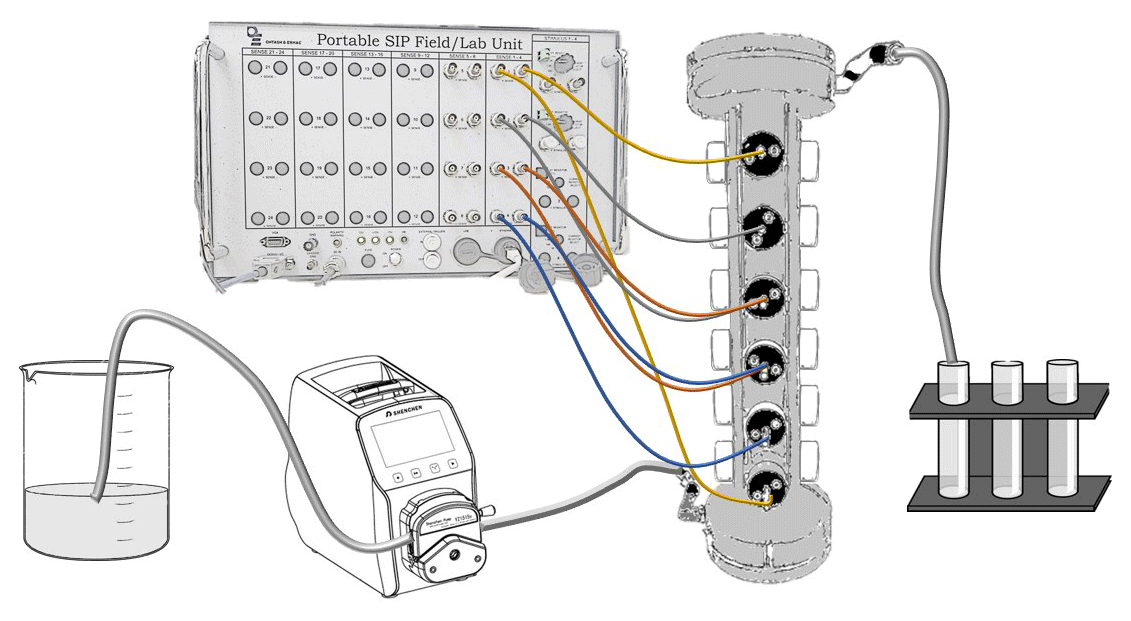
Figure 1 Laboratory setup: the inflow solution is pumped into the column from its bottom, and the outflow is collected in fractions. SIP signal is measured between three sets of potential electrodes: channel 1 (blue), channel 2 (orange) and channel 3 (grey). The current is injected between the top and bottom electrodes (yellow).

To link between surface processes (specifically, the characteristics of the EDL) during the SIP measurement and the complex conductivity signal, the Nernst–Plank equation should be solved, considering the influence of the external electric field expressed by Ohm's law. The resulting expression connects the mobility of ions in the Stern layer to the complex surface conductivity (Leroy and Revil, 2009).

$$\begin{array}{}\text{(3)}& {\mathit{\sigma }}_s^{*}={\displaystyle \frac{\mathrm{2}}{r_{\mathrm{0}}}}\left({\mathrm{\Sigma }}_{\mathrm{s}}+{\mathrm{\Sigma }}_{\mathrm{d}}\right)-{\displaystyle \frac{\mathrm{2}}{r_{\mathrm{0}}}}{\displaystyle \frac{{\mathrm{\Sigma }}_{\mathrm{s}}}{\mathrm{1}+i\mathit{\omega }{\mathit{\tau }}_{\mathrm{0}}}},\end{array}$$

where r₀ (m) is the grain radius, Σ_s (S) is the conductance of the Stern layer, Σ_d (S) represents the contribution of the diffuse layer, f (Hz) is the frequency, ω=2πf (rad s⁻¹) is the angular frequency of the current, ${\mathit{\tau }}_{\mathrm{0}}=\frac{r_{\mathrm{0}}^{\mathrm{2}}}{\mathrm{2}{D}^{*}}$ is the relaxation time constant (s) and D^* (m² s⁻¹) is the diffusion coefficient of the counter ion in the Stern layer.

Both Σ_s and Σ_d are related to the mobility of ions in the EDL. Under the assumption that only one species is adsorbed to the mineral surface (i.e., mono-ionic system) and that the electrolyte is composed of N species, the Stern and diffuse layer conductance are given by

$$\begin{array}{}\text{(4)}& {\displaystyle }{\mathrm{\Sigma }}_{\mathrm{s}}=e\mathrm{|}z\mathrm{|}\mathit{\beta }{\mathrm{\Gamma }}_{\mathrm{s}}\text{(5)}& {\displaystyle }{\mathrm{\Sigma }}_{\mathrm{d}}=e{\mathrm{\Sigma }}_{j=\mathrm{1}}^N\mathrm{|}{z}_j\mathrm{|}{\mathit{\beta }}_j{\mathrm{\Gamma }}_{j,\mathrm{d}},\end{array}$$

where e = 1.6 × 10⁻¹⁹ C is the elementary charge, z is the valence of the ion, β (${\mathrm{m}}^{\mathrm{2}}{\mathrm{s}}^{-\mathrm{1}}{\mathrm{V}}^{-\mathrm{1}}$) is the ion mobility and Γ_s (1 m⁻²) and Γ_d (1 m⁻²) are the surface site densities of the Stern and diffuse layer, respectively.

2.2 Flow-through experiments

The laboratory setup included a polycarbonate column (3 cm inner diameter, 32 cm long) equipped with six brass electrodes at equal spacing of 4 cm. The top and the bottom electrodes were used to inject the electrical current into the soil profile (and were fully penetrating the soil column), and the remaining four electrodes were used to measure the potential between each pair. The soil column was connected through the electrodes to a portable SIP device (Ontash and Ermac Inc., NJ) using alligator clips. Inflow solution entered the column through its bottom using a peristaltic pump to create saturated flow (a constant flow of 1.3 mL min⁻¹), and outflow fractions were collected (see Fig. 1).

Four experiments were performed: (a) CaCl₂ transport through a loamy profile, (b) CaCl₂ transport through a sandy profile, (c) ZnCl₂ transport through a sandy profile and (d) CaCl₂ transport through a layered profile that included the same loamy soil used for (a) but had a 3 cm sand layer in the middle. Throughout the experiments, the SIP signal was recorded at frequencies of 0.1–10 000 Hz. The impedance and phase shift data were used to calculate the real and imaginary conductivity. Additional information regarding the soil composition and column packing is in Sect. S1 in the Supplement.

Figure 2 Real (a) and imaginary (b) conductivity between 0.1 and 1000 Hz at five different times (∼ 0.5, ∼ 1, ∼ 1.5, ∼ 2, ∼ 3 h) for the loamy soil. The inserts in (a) and (b) schematically present the dynamics of the real and imaginary conductivity at 1 Hz. Panel (c) shows the imaginary conductivity of the three soils used in this work: loamy soil, sand (untreated; used for the heterogeneous experiment) and treated sand.

Prior to each experiment, a 200 mg L⁻¹ NaCl background solution was injected into the column. The background solution injection proceeded until equilibrium between the inlet and the outlet EC was obtained. Subsequently to the EC stabilization, the inflow background solution was replaced by either 360 mg L⁻¹ CaCl₂ solution or 360 mg L⁻¹ ZnCl₂ solution. The replacement of the background solution by the CaCl₂ or ZnCl₂ solutions marked the beginning of the experiments (t=0).

2.3 Soil preparation and characterization

Red loamy soil (denoted here as “loamy soil”; used for experiments (a) and (d)) and the sand used for the heterogeneous experiment (d) were air-dried, passed through a < 250 µm sieve and used without further treatment. The sandy soil that was used for both CaCl₂ and ZnCl₂ transport (experiments (b) and (c)) was treated to remove its CaCO₃ content prior to the column packing. Briefly, the soil was mixed with hydrochloric acid under stirring conditions and then washed with deionized water (DW) three times. Then, it was left overnight in a diluted NaOH solution (pH = 8). Finally, the soil was washed and left overnight in an NaCl solution (0.5 g L⁻¹) and then air-dried and packed. The texture of the loam and the sand was determined using a hydrometer experiment (based on Stokes' law; Bouyoucos, 1962), and the CEC of the loam, sand and treated sand was measured using the BaCl₂ compulsive exchange method (Gillman and Sumpter, 1986).

2.4 Complementary analysis

The outflow solution was collected in equal volume fractions. Immediately after the collection of each sample, its EC was measured using an EC meter (Eutech con 700). Each sample was then passed through a 0.22 µm cellulose filter and analyzed for Cl⁻ using an ion chromatograph (881 compact IC pro, Methrohm) and for sodium, calcium and zinc by an inductively coupled plasma–optical emission spectrometer (ICP-OES; iCAP 6000).

2.5 Modeling

A simple solute transport model was constructed based on the HYDRUS 1D platform (Simunek et al., 1998). HYDRUS 1D is a computer program for the numerical modeling of water flow and solute transport in porous media. The inverse tool of HYDRUS 1D was applied to fit model parameters to experimental results, based on the Levenberg–Marquardt nonlinear minimization method (Marquardt, 1963). The appropriate mass balance equation for this application is given by the advection–dispersion equation (ADE)

$$\begin{array}{}\text{(6)}& {\displaystyle \frac{\partial c}{\partial t}}+{\displaystyle \frac{{\mathit{\rho }}_{\mathrm{b}}}{\mathit{\theta }}}{\displaystyle \frac{\partial \widehat{c}}{\partial t}}={\displaystyle \frac{\partial }{\partial l}}\left(D_{\mathrm{h}}{\displaystyle \frac{\partial c}{\partial l}}\right)-{\displaystyle \frac{\partial }{\partial l}}\left(\mathit{\nu }c\right),\end{array}$$

where c (g cm⁻³) is the dissolved species concentration t (h) is time, l (cm) is the vertical coordinate, v (cm h⁻¹) is the water velocity, $D_{\mathrm{h}}=\mathit{\alpha }\mathit{\nu }+D$ is the hydrodynamic dispersion coefficient (cm² h⁻¹), α (cm) is the dispersivity, D (cm² h⁻¹) is the diffusion coefficient, ρ_b is the soil bulk density (g cm⁻³) and $\widehat{c}$ is adsorbed concentration (g g⁻¹) that can be expressed in terms of c using an adsorption isotherm. For simplistic linear adsorption model, $\widehat{c}$ can be expressed as

$$\begin{array}{}\text{(7)}& \widehat{c}=K_{\mathrm{d}}c,\end{array}$$

where K_d (cm³ g⁻¹) is the linear adsorption coefficient, which is equal to 0 for non-reactive solutes.

Here, we considered saturated flow; the boundary flux was determined based on the measured flow. The dispersivity (α) and the soil porosity (n) were fitted using the inverse tool for the non-reactive solutes. For the reactive species (Ca²⁺ or Zn²⁺) model fitting process, the obtained values of n and α values were used, and the adsorption coefficient K_d was fitted.

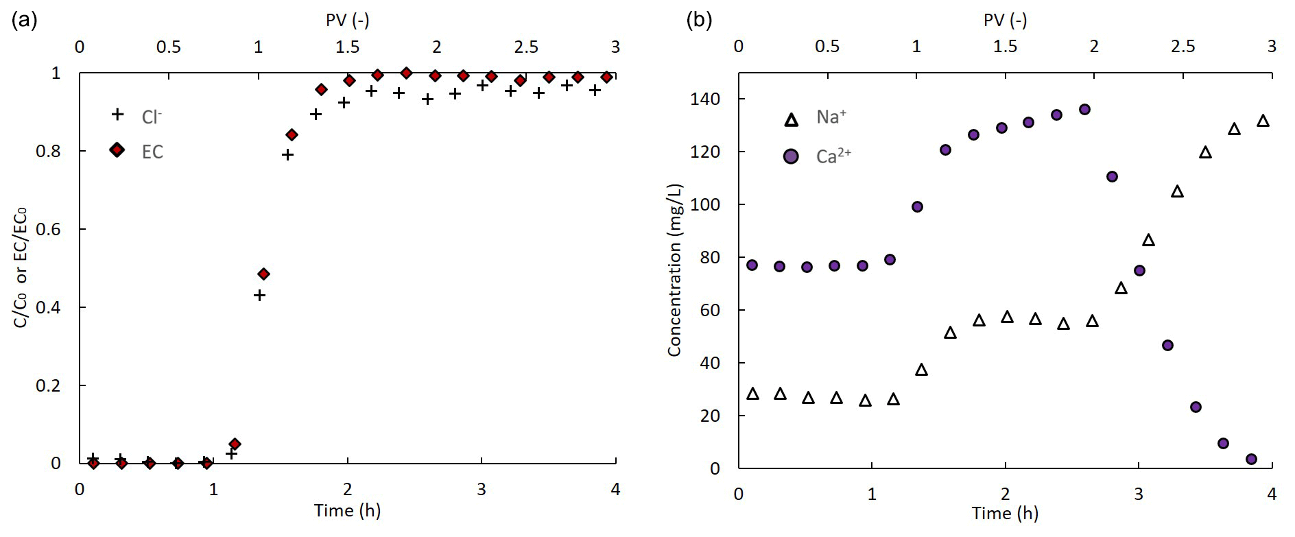
Figure 3 Outflow values vs. time (bottom horizontal axis) and pore volume (PV; upper horizontal axis) of (a) measured Cl⁻ and EC ((+) signs and red rhombi) and (b) Na⁺ and Ca²⁺ ions (empty triangles and purple circles).

3 Results and discussion

3.1 SIP spectra and temporal response analysis

The complex conductivity measurements obtained by SIP hold information regarding the soil's pore-water conductivity and its surface polarization in response to the applied external field. Figure 2a and b present σ^′ and σ^′′ between 0.1 and 1000 Hz at five different times for a loamy soil profile during continuous CaCl₂ injection. The CaCl₂ solution had a higher EC compared to the background solution, and hence σ^′ increases accordingly as the inflow solution progressed along the column. The σ^′′ spectra present a sharp polarization peak at ∼ 1 Hz, and its magnitude increases and then decreases in response to the introduction of the inflow CaCl₂ solution. A relaxation model fit (Pelton et al., 1979) revealed a mild change in relaxation time between the beginning and the end of the CaCl₂ injection (from 0.16 to 0.18 s; not presented). The inserts in Fig. 2a and b schematically present the values of the real and imaginary conductivity at 1 Hz vs. time (note the BT pattern received for the σ^′ vs. time graph). Figure 2c shows σ^′′ between 0.1 and 1000 Hz for the three soils used in this work: loamy soil, sand (untreated; used for the heterogeneous experiment) and sand that was treated with acid to remove its CaCO₃ content. While all three spectra present a polarization peak at ∼ 1 Hz, they differ in their magnitude. The loamy soil's σ^′′ magnitude is considerably higher compared to the sand along the measured frequency range. This is explained by the larger clay fraction and higher CEC of the loam compared to the sand that have been shown to affect the magnitude of σ^′′ (Revil, 2012). The CEC of the three soils is ∼ 5, ∼ 4.15 and ∼ 3.75 meq (100 g)⁻¹ for the loam, sand and treated sand, respectively.

3.2 CaCl₂ transport and ${\mathrm{Na}}^{+}-{\mathrm{Ca}}^{\mathrm{2}+}$ exchange in a homogeneous loamy profile

Figure 3a presents the measured outflow Cl⁻ concentrations and EC values vs. pore volume (PV (–); one pore volume is equivalent to ∼ 82 min). Both the Cl⁻ and EC outflow values along time fit the expected BT pattern of a non-reactive solute: the ratio of solute concentration (C) to its inflow concentration (C₀) is equal to $\frac{\mathrm{1}}{\mathrm{2}}$ approximately after one PV ($\text{PV}(\frac{C}{C_{\mathrm{0}}}=\frac{\mathrm{1}}{\mathrm{2}})\approx \mathrm{1}$). Na⁺ and Ca²⁺ dynamics during the CaCl₂ injection are described in Fig. 3b. Na⁺ outflow concentrations increased in parallel to the increase in outflow Cl⁻. This observation is explained by the fact that the injection of the CaCl₂ solution started after an equilibrium between the background solution and the soil was reached. At this point, the Na⁺ concentration in the pore water was already equal to its concentration in the inflow solution ($\frac{C}{C_{\mathrm{0}}}=\mathrm{1}$), and therefore Na⁺ behaved as a non-reactive solute. As the CaCl₂ solution entered the column, adsorbed Na⁺ ions were replaced by Ca²⁺, and hence the Na⁺ outflow concentration increased further. In parallel to the increase in outflow Na⁺, a moderate increase in outflow Ca²⁺ was observed. This early increase in outflow Ca²⁺ represents the fraction of the inflow Ca²⁺ ions that did not participate in the ${\mathrm{Na}}^{+}-{\mathrm{Ca}}^{\mathrm{2}+}$ exchange reaction (note the timing at ∼ one PV). Subsequently to the completion of the ${\mathrm{Na}}^{+}-{\mathrm{Ca}}^{\mathrm{2}+}$ exchange, a decrease in outflow Na⁺ concentrations was observed, while outflow Ca²⁺ increased and reached its inflow concentration.

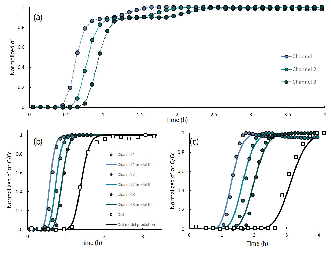
Figure 4 (a) Real conductivity at 1 Hz vs. time at three locations, (b) model fit to the σ^′-based initial BT and model prediction for the non-reactive species at the outflow compared to their measured concentration and (c) model fit to the σ^′-based secondary BT and model prediction for the reactive fraction of Ca²⁺ ions (calculated as outflow Ca²⁺ minus its “non-reactive fraction”) compared to its measured concentration.

Outflow EC values (Fig. 3a) increased in a similar pattern to the Cl⁻ ions and reached their maximal value after ∼ 1.3 PVs. The major changes in the ionic composition of the outflow during the ${\mathrm{Na}}^{+}-{\mathrm{Ca}}^{\mathrm{2}+}$ exchange reaction (see Fig. 3b) were not reflected in the EC measurements. This observation is consistent with the findings of Shackelford et al. (1999); in their study, they combined experimental observations and a theoretical approach to investigate EC-based BTCs. They used a sodium-saturated clay soil (sodium bentonite) and a CaCl₂ solution as the inflow solution. Their results showed that while the EC-based BTC matched the Cl⁻ BT pattern, reaching its maximal value after ∼ 1.5 PVs, it stayed stable afterwards and did not reflect the subsequent decrease in outflow Na⁺ and increase in outflow Ca²⁺, similarly to the results presented here.

Figure 4a presents the normalized real component of the complex conductivity at 1 Hz vs. time at three locations denoted as channel 1, channel 2 and channel 3, for the homogeneous loamy profile. The σ^′ values were normalized by subtraction of the minimal value and division by the difference between the maximal and minimal value (normalized ${\mathit{\sigma }}^{\prime }=\frac{{\mathit{\sigma }}^{\prime }-{\mathit{\sigma }}_{min}^{\prime }}{{\mathit{\sigma }}_{max}^{\prime }-{\mathit{\sigma }}_{min}^{\prime }}$). The values of the real conductivity along time depicted the general shape of a BTC: a gradual increase in σ^′ was followed by stabilization of the signal around its maximal value. The σ^′-based BT pattern at the different channels was consistent with the location of the electrode pairs: BT was first observed at channel 1, which is the closest to the inlet, then at channel 2 and lastly at channel 3. Further, the values of σ^′ along time are in agreement with the measured EC values presented in Fig. 3a. In all three channels, the signal was initially stable at around 580 µS cm⁻¹ and stabilized on its maximal value (${\mathit{\sigma }}_{\mathrm{0}}^{\prime }$) at ∼ 1055 µS cm⁻¹. Interestingly, a secondary BT pattern was detected in the σ^′-based curves between 0.9 and 2.5 h. The temporal location of this BT pattern suggests that the real part of the complex conductivity responded to the increased pore-water Ca²⁺ concentrations after the ${\mathrm{Na}}^{+}-{\mathrm{Ca}}^{\mathrm{2}+}$ exchange reaction reached equilibrium. This increase, however, occurred simultaneously to the decrease in Na⁺ concentrations in the pore water and hence did not have a major effect on the ionic strength of the outflow and was not detected by the EC measurements (see Fig. 3a).

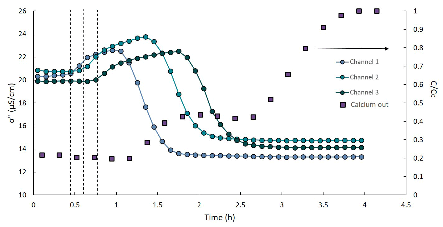
Figure 5 Imaginary conductivity at 1 Hz vs. time at three locations (left vertical axis) and outflow ${\mathrm{Ca}}^{\mathrm{2}+}/{\mathrm{Ca}}_{\mathrm{0}}^{\mathrm{2}+}$ vs. time (right vertical axis). The vertical dashed lines represent the beginning of the increase in σ^′′ at each of the channels.

A HYDRUS 1D-based model was constructed and calibrated separately for the transport of the non-reactive (Cl⁻, Na⁺ and a small fraction of the Ca²⁺ that reached the outlet of the column at the same time as the non-reactive Cl⁻ and Na⁺ ions) and the reactive (Ca²⁺ minus the “non-reactive fraction”) ions in the system. In the model fitting process, the σ^′ time series were used as a proxy for concentration. This approach was used before; Moreno et al. (2015) used electrical resistivity tomography (ERT) to monitor the water dynamics under a drip-irrigated citrus orchard. They presented a coupled flow and transport model that was calibrated using electrical conductivity measurements with the pore-water electrical conductivity serving as a pseudo-solute.

Here, the σ^′-based BTCs of all three channels were split into two parts, separating the initial and the secondary BT. Each part was then used separately for the model calibration: the initial BT data were used for the calibration of the non-reactive solute transport, and the secondary BT data were used for the reactive solute transport. The “splitting point” of the data for each channel was determined according to the value of the curve's slope between 0.5 and 1.5 h (i.e., the data were split at the point of minimal slope). The obtained data sets were normalized to a scale of 0 to 1, and the HYDRUS inverse tool was used to fit the model parameters. The obtained dispersivity and porosity were 0.26 cm and 47 %, respectively. For the reactive ion, a K_d value of 2.5 cm³ g⁻¹ was obtained.

Figure 4b and c present the normalized σ^′-based time series and their model fit for the non-reactive and reactive ions, respectively. Using the obtained model parameters, outflow ion concentrations were predicted (black continuous line) and compared to the measured concentrations (clear rectangles). Both the model fit and the predicted outflow concentrations present an excellent fit to the measured data. R² for the non-reactive ions is 0.991 and 0.972, respectively, and 0.972 and 0.965, respectively, for the reactive ion. The ability to accurately predict the BT pattern of outflow concentrations using a simple, HYDRUS-based numerical model suggests that the electrical measurement can replace outflow sampling and chemical analysis. Clearly, in more complex systems that involve multiple ions (either in the inflow solution or adsorbed to the soil), some sampling and chemical analysis may be required in addition to the SIP monitoring. However, even for such systems, the use of electrical monitoring may allow the sampling frequency to be drastically reduced and the analysis performed on the outflow samples to be simplified.

The imaginary conductivity along time (Fig. 5) provides a clear indication for the scope of the ${\mathrm{Na}}^{+}-{\mathrm{Ca}}^{\mathrm{2}+}$ exchange reaction. The signal increased initially in all channels but decreased and stabilized after reaching its maximal value. The observed decrease in σ^′′ that was followed by the BT of Ca²⁺ at the outflow is related to the altered composition of the Stern layer after the exchange reaction. Imaginary conductivity changes have been shown to be related to the mobility of ions in the Stern layer (Vaudelet et al., 2011; Schwartz et al., 2012). Specifically, adsorbed Na⁺ ions maintain their hydration shell and, hence, are weakly adsorbed to the soil and are more mobile compared to Ca²⁺. During the ${\mathrm{Na}}^{+}-{\mathrm{Ca}}^{\mathrm{2}+}$ exchange, the less mobile Ca²⁺ ions occupied the Stern layer and caused the decrease in σ^′′. These observations are consistent with earlier studies. Shefer (2015) examined the SIP signature of ion exchange processes in loam and loess soils. The soil profiles were treated with high concentrations of NaCl or CaCl₂ solution to alter the ionic composition of the Stern layer. Her results showed that the imaginary conductivity of the soil profile increased inversely to the mobility of the adsorbed ion. Vaudelet et al. (2011) observed similar results comparing the SIP signal of a saturated sand profile adsorbed with Cu²⁺ and Na⁺. The Cu²⁺ ions are adsorbed to the soil mainly as an inner sphere (less mobile) species, and hence the ${\mathrm{Na}}^{+}-{\mathrm{Cu}}^{\mathrm{2}+}$ exchange reduced the overall ion mobility in the Stern layer, similarly to the ${\mathrm{Na}}^{+}-{\mathrm{Ca}}^{\mathrm{2}+}$ exchange considered here.

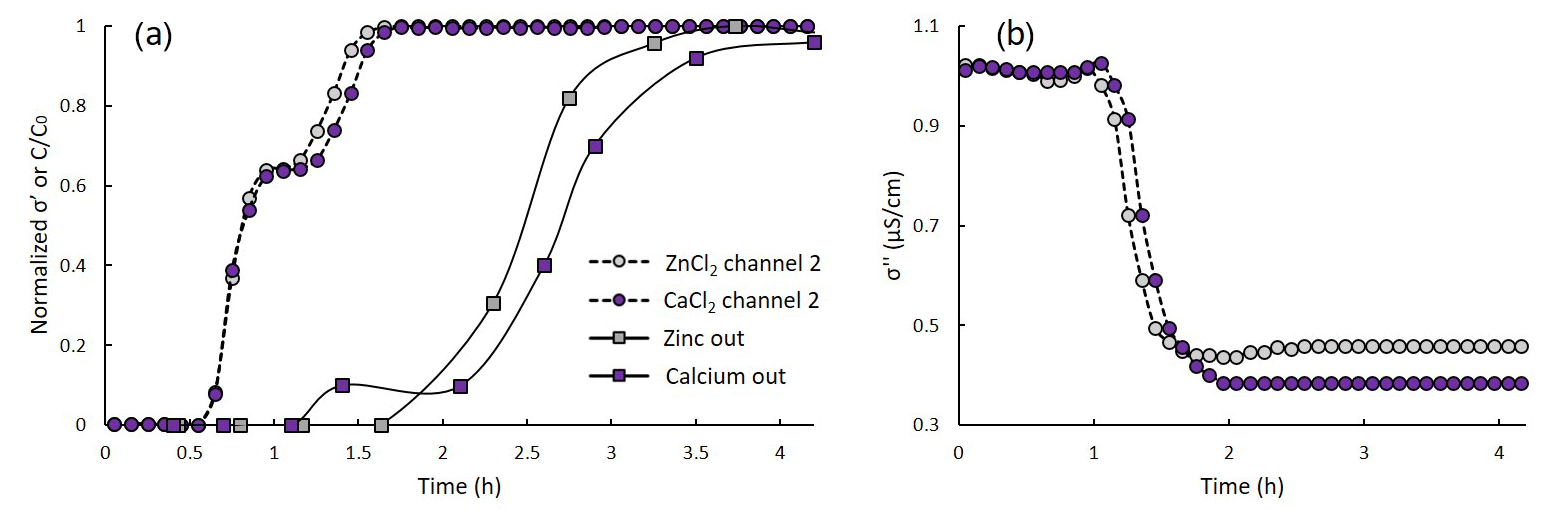
Figure 6 Normalized real conductivity (a) and imaginary conductivity (b) vs. time at 1 Hz vs. (channel 2) for CaCl₂ and ZnCl₂ transport in a homogeneous sandy profile. The rectangular markers symbolize the measured outflow Zn²⁺ and Ca²⁺ concentrations.

The increase in σ^′′ began before PV = 1 at each of the channels was reached (see dashed vertical lines in Fig. 5) and, hence, might be related to the progression of the non-reactive ions' front and increase in EC during the CaCl₂ injection. However, the imaginary conductivity is only marginally influenced by the conductivity of the pore water. Moreover, the signal continued to increase in all channels after the stabilization of the outflow EC. This may imply that the increase in σ^′′ is related to the ${\mathrm{Na}}^{+}-{\mathrm{Ca}}^{\mathrm{2}+}$ exchange reaction. As CaCl₂ entered the column, Na⁺ ions leave the Stern layer, while Ca²⁺ ions enter it. The SIP results (the observed increase in σ^′′) suggest that there is an intermediate stage at which neither Ca²⁺ nor Na⁺ are fully adsorbed, which means that their mobility is higher than their mobility at the Stern layer (Eqs. 3–4). Considering a simple EDL model, this suggests that both the Ca²⁺ and Na⁺ are still present in the diffuse layer. This suggests that the beginning of the σ^′′ increase indicates the initiation of the exchange reaction at each location, while the steep decrease and following stabilization of the signal on its minimal value marks the end of the exchange. The secondary BT pattern observed in the σ^′ signal (see Fig. 4b) supports our hypothesis: the minimal σ^′′ values (indicating the end of the ${\mathrm{Na}}^{+}-{\mathrm{Ca}}^{\mathrm{2}+}$ exchange) were observed at the same time as the stabilization of the σ^′ signal on its maximal value (suggesting the presence of Ca²⁺ at its inflow concentration in the pore water).

The role of σ^′′ as an indicator of the ${\mathrm{Na}}^{+}-{\mathrm{Ca}}^{\mathrm{2}+}$ exchange progression suggests that the σ^′′ values can serve as a proxy for the adsorbed concentration of the retarded (reactive) species in an alternative modeling approach. A demonstration of this approach and a technical description of the model construction and calibration are presented in the Supplement (Sect. S2). However, the initial increase in σ^′′ during the exchange process is not captured by this simple model. Since this increase is assumed to be related to non-equilibrium processes, to fully connect the SIP data to the ${\mathrm{Na}}^{+}-{\mathrm{Ca}}^{\mathrm{2}+}$ exchange, a more complex model that includes these processes should be constructed.

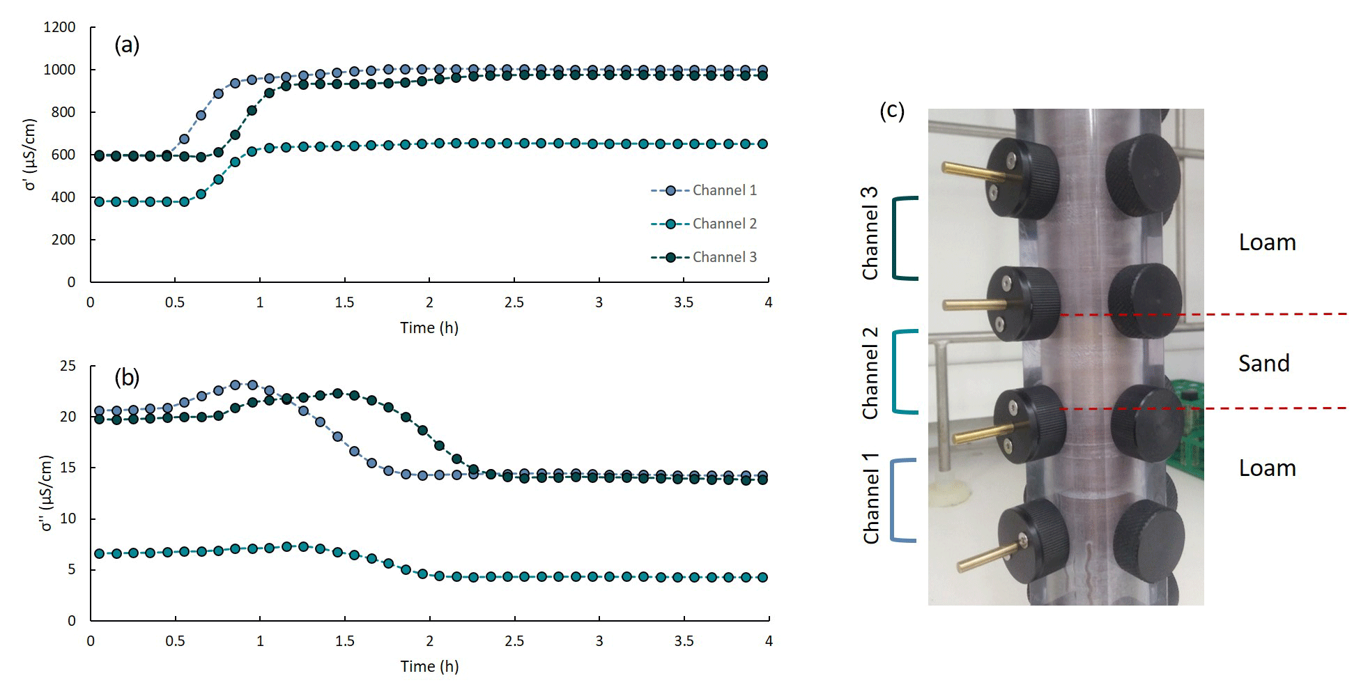
Figure 7 The real (a) and imaginary (b) components of the complex conductivity at 1 Hz vs. time, for the heterogeneous profile. Panel (c) shows the heterogeneous profile: a sandy layer was packed between the two middle electrodes (channel 2).

3.3 CaCl₂ and ZnCl₂ transport in a homogeneous sandy profile

Similarly to the observed for the loamy profile, a double BT pattern was observed for the transport of CaCl₂ and ZnCl₂ in a sandy profile. Figure 6a presents the normalized real conductivity (at 1 Hz) recorded in channel 2 vs. time, for the CaCl₂ and ZnCl₂ transport experiments (purple and grey circles). It also shows the measured outflow values of Ca²⁺ and Zn²⁺ as was measured by ICP (purple and grey squares). The initial BT observed between 0 and 1 h was nearly identical for both experiments (CaCl₂ or ZnCl₂ injection). Both experiments were performed on the same soil and started after an equilibrium with the same background solution was reached. Further, the initial BT indicates the movement of the non-reactive ions which are expected to progress at a similar rate in both cases. The secondary BT, however, was slightly earlier for the ZnCl₂ case, suggesting that calcium is retained for longer in the soil compared to zinc; this is also evident by the measured outflow concentrations. In the pH range characteristic to soil systems, both calcium and zinc are found in the soil in their divalent form. However, in the presence of Cl⁻, OH⁻ and the carbonate system's ions, a number of complexes are formed. To explain the delayed BT of the calcium compared to the zinc, PhreeqC simulations were performed (Parkhurst, 1995). The simulations calculated the concentrations of the possible calcium and zinc complexes in the characteristic pH of the system and in equilibrium with atmospheric CO₂. It was found that for our system, while calcium was mostly present in its divalent form (< 97 % of its total concentration), around 13 % of the zinc was present in a monovalent form (as ${\mathrm{ZnHCO}}_{\mathrm{3}}^{+}$). The stronger attachment of the Ca²⁺ ions to the soil is also evident by the σ^′′ temporal variation presented in Fig. 6b. For both experiments, the σ^′′ values drop in response to the Na−Ca or Na−Zn exchange. However, the values drop lower in the case of the ${\mathrm{Na}}^{+}-{\mathrm{Ca}}^{\mathrm{2}+}$ exchange, indicating lower ion mobility in the soil's EDL after the exchange. HYDRUS-based transport models were calibrated for both experiments based on the σ^′ time series and presented an excellent prediction of the outflow concentrations (model fit and prediction for the ZnCl₂ is presented in Sect. S3 in the Supplement). The obtained dispersivity and porosity were 0.25 cm and 48 %, respectively. K_d values of 2.13 and 2.2 cm³ g⁻¹ were obtained for the zinc and the calcium, respectively.

3.4 CaCl₂ transport and ${\mathrm{Na}}^{+}-{\mathrm{Ca}}^{\mathrm{2}+}$ exchange in a heterogeneous profile

A comparison of Ca²⁺, Na⁺ and Cl⁻ concentrations and EC values at the outflow samples collected during the heterogeneous and homogeneous experiments revealed no significant difference (t test, α = 0.01; see Sect. S4 in the Supplement). This may be due to a combination of several different reasons: first, the loamy soil used here contained > 90 % sand, and hence the overall difference in CEC between the profiles was minor. Further, the sand layer was relatively thin at one-tenth of the profile's total volume (see Fig. 7c). Since the chemical measurements were conventionally performed on outflow samples, the obtained transport patterns of the different ions along time represent a spatial average, and hence the implications of the heterogeneity were not detected by the chemical analysis.

Figure 7 presents the real (Fig. 7a) and imaginary (Fig. 7b) components of the complex conductivity at 1 Hz vs. time for the heterogeneous profile. Similarly to the homogeneous experiment, the σ^′-based BT pattern observed between 0.5 and 1.2 h appeared at the different channels according to the geometrical hierarchy. The general shapes of the secondary increase in σ^′ (between 0.9 and 2.5 h) and the imaginary conductivity curves are also consistent with the homogeneous case. However, for both components of the complex conductivity, the signal recorded in the middle channel (channel 2, measuring over the sand portion of the column) was notably lower compared to the other two channels. σ^′ values ranged between 600–1055 µS cm⁻¹ in the loam but were between 400–600 µS cm⁻¹ in the sandy layer. Similarly, σ^′′ values ranged between 15–24 µS cm⁻¹ in the loam compared to 4–7 µS cm⁻¹ in the sandy layer. This observation indicates that the SIP-based BTC can characterize system heterogeneity, which is a major advantage over the conventional outflow analysis method.

The sensitivity of the complex conductivity to the geometry of the porous media and its surface charge means that differences in soil grain size, porosity and CEC are likely to be reflected in the obtained signal. Geo-electrical studies of porous media characteristics mostly focused on physical aspects, rather than chemical aspects. The effect of soil hydraulic characteristics on its SIP signature has been studied before (e.g., Kruschwitz et al., 2010; Breede et al., 2012; Nordsiek et al., 2016). For example, Kruschwitz et al. (2010) examined the low-frequency electrical spectra of a range of natural and artificial porous media with the aim to link the electrical signature to the physical properties of the examined media. They confirmed a significant positive correlation between the electrical polarization and the surface area to pore volume ratio. Breede et al. (2012) investigated the SIP signature of sand and sand–clay mixtures (5, 10 and 20 % clay) under different saturation levels. Their results showed that the magnitude of both σ^′ and σ^′′ were lower in sand compared to sand–clay mixtures for saturated conditions. The distinct values of σ^′ and σ^′′ measured in channel 2 suggest that this area has different hydraulic characteristics compared to the rest of the profile. Specifically, it is consistent with the presence of a coarser textured soil, characterized by larger average grain size and lower CEC compared to the loamy soil that was measures by channels 1 and 3.

Analysis of the magnitude of the initial increase in σ^′′ at the different channels (between 0.5 and 1.6 h) for the heterogeneous case showed that it was lower in the sandy layer (channel 2) compared to the loam (channels 1 and 3) by ∼ 15 %. This observation can be explained by the difference in CEC between the different soil types (a difference of 17 %; see Sect. 3.1). Isomorphic exchange in the mineral structure is less substantial in sand, which, in combination with its smaller specific surface area, leads to lower CEC. Hence, the changes to the Stern layer composition resulting from the ${\mathrm{Na}}^{+}-{\mathrm{Ca}}^{\mathrm{2}+}$ exchange were less prominent in the sand.

4 Summary and conclusions

The main objective of this study was to demonstrate the ability of SIP measurements to depict BT patterns, ion exchange processes and profile heterogeneity in a simple system. The presented laboratory setup combines geo-electrical measurements backed by standard outflow EC and chemical analysis. Four experimental cases were examined: CaCl₂ transport through a homogeneous loamy profile, CaCl₂ and ZnCl₂ transport through a homogeneous sandy profile and CaCl₂ transport through a heterogeneous profile. Our results led us to the following conclusions: (1) SIP may serve as an alternative or supplementary tool for the monitoring of solute transport patterns through porous media in simple systems, requiring no outflow sampling. (2) In addition to the changes in outflow EC, the SIP measurement indicated the initiation and the end of the cation exchange along the soil column and, following it, the delayed BT of the cations. (3) SIP-based BTC analysis is superior over conventional outflow analysis as it can characterize system heterogeneity and is superior over EC-based analysis as it is capable of distinction between the adsorption end-members. Clearly, for more complex systems that involve multiple ions (either in the inflow solution or initially adsorbed to the soil) and additional processes (such as dissolution or biochemical reactions), SIP alone may not be sufficient for full resolution of the system, and some sampling and chemical analysis may be required. However, even for such systems, the use of electrical monitoring may not only allow us to reduce the sampling frequency and types of analysis performed on the outflow samples, but also infer spatial heterogeneity and more complex processes than what can be achieved by outflow sampling alone. Remaining challenges include the development of appropriate methodology that combines SIP and EC/chemical-based BT analysis for complex systems and the upscaling of this approach to field BT analysis.