the Creative Commons Attribution 4.0 License.
the Creative Commons Attribution 4.0 License.
 | 26 May 2021
Technical note: Evaluation and bias correction of an observation-based global runoff dataset using streamflow observations from small tropical catchments in the Philippines
Carlos Primo C. David
Pamela Louise M. Tolentino
Even in relatively wet tropical regions, seasonal fluctuations in the water cycle affect the consistent and reliable supply of water for urban, industrial, and agricultural uses. Historic streamflow monitoring datasets are crucial in assessing our ability to model and subsequently plan for future hydrologic changes. In this technical note, we evaluate a new observation-based global product of monthly runoff (GRUN; Ghiggi et al., 2019) for 55 small tropical catchments in the Philippines with at least 10 years of data, extending back to 1946 in some cases. Since GRUN did not use discharge data from the Philippines to train or calibrate their models, the data presented in this study, 11 915 monthly data points, provide an independent evaluation of this product. We demonstrate across all observations a significant but weak correlation (r2=0.372) between the GRUN-predicted values and observed river discharge, as well as somewhat skillful prediction (volumetric efficiency = 0.363 and log(Nash–Sutcliffe efficiency) = 0.453). GRUN performs best among catchments located in climate types III (no pronounced maximum rainfall with short dry season) and IV (evenly distributed rainfall, no dry season). There was a weak negative correlation between volumetric efficiency and catchment area, and there was a positive correlation between volumetric efficiency and mean observed runoff. Further, analysis for individual rivers demonstrates systematic biases (over- and underestimation) of baseflow during the dry season and underprediction of peak flow during some wet months for most catchments. To correct for underprediction during wet months, we applied a log-transform bias correction which greatly improves the nationwide root mean square error between GRUN and the observations by an order of magnitude (2.648 mm d−1 vs. 0.292 mm d−1). This technical note demonstrates the importance of performing such corrections when determining the proportional contribution of smaller catchments or tropical islands such as the Philippines to global tabulations of discharge. These results also demonstrate the potential use of GRUN and future data products of this nature after consideration and correction of systematic biases to (1) assess trends in regional-scale runoff over the past century, (2) validate hydrologic models for unmonitored catchments in the Philippines, and (3) assess the impact of hydrometeorological phenomena to seasonal water supply in this wet but drought-prone archipelago.
- Article
(5083 KB) - Full-text XML
-
Supplement
(3839 KB) - BibTeX
- EndNote


The global water crisis affects an estimated two-thirds of the world's population and is considered one of the three biggest global issues that we need to contend with (Kummu et al., 2016; WEF, 2018). The most important source of freshwater in terms of use is surface water. It is the primary resource for irrigation and industrial use and provides the bulk of water supply for many large cities. Long-term streamflow datasets are useful for resource management and infrastructure planning (e.g., Evaristo and McDonnell, 2019). Such data are even more critical in areas that rely on run-of-the-river flow and do not use storage structures, such as dams and impoundments. Further, a robust long-term dataset is crucial in the face of increased variability in stream discharge due to land use change, increased occurrence of mesoscale disturbances, and climate change (e.g., Abon et al., 2016; David et al., 2017; Kumar et al., 2018). In the absence of long-term streamflow datasets for most locations in the world, several researchers have compiled datasets worldwide that are used to estimate streamflow in ungauged areas (Meybeck et al., 2013; Gudmundsson et al., 2018; Do et al., 2018; Alfieri et al., 2020; Harrrigan et al., 2020). Several global hydrological models have also been created to project variations in streamflow and extend present-day measurements to the future (Hagemann et al., 2011; Davie et al., 2013; Winsemius et al., 2016). A recent contribution to modeled global runoff products is the Global Runoff Reconstruction (GRUN) (Ghiggi et al., 2019). GRUN is a global gridded reconstruction of monthly runoff for the period 1902–2014 at 0.5∘ (∼50 km by 50 km) spatial resolution. It used global streamflow data from 7264 river basins that train a machine-learning algorithm that inferred runoff generation processes from precipitation and temperature data.
There is a disparity in the availability of long-term gauged river datasets between continental areas and smaller island nations, which have more dynamic hydrometeorologic system owing to the size of the catchments and proximity to the ocean (e.g., Abon et al., 2011; Paronda et al., 2019). As a result, information from island nations is usually not used to train or evaluate global models. The Philippines offers a unique example where manual stream-gauging programs have started in 1904 and, while spotty at times, have continued to today. This island nation on the western side of the Pacific Ocean is characterized by a very dynamic hydrologic system because it is affected by tropical cyclones, seasonal monsoon rains, subdecadal cycles such as the El Niño–Southern Oscillation (ENSO) and climate change (Abon et al., 2016; David et al., 2017; Kumar et al., 2018). The impact of climate change on the hydrological cycle can be observed the most for tropical island nations, including the Philippines (Nurse et al., 2014).
This technical note evaluates the accuracy of the GRUN dataset (GRUN_v1) as applied to the hydrodynamically active smaller river basins in the Philippines. Additionally, it explores the possible hydrologic parameters that may need to be considered and/or optimized so that such global datasets can predict runoff in smaller, ungauged basins more accurately.
2.1 Climate types
The Philippines has four climate types (see also Abon et al., 2016; Tolentino et al., 2017; Fig. 1): type I climate on the western seaboard of the Philippines is characterized by distinct wet (May to October) and dry (November to April) seasons; type II climate on the eastern seaboard has no distinct dry period with maximum rainfall occurring from November to February; type III inland climate experiences less annual rainfall with a short dry season (December to May) and a less pronounced wet season (June to November); and type IV southeast inland climate receives less rainfall and is characterized by an evenly distributed rainfall pattern throughout the year.
2.2 Historical streamflow data
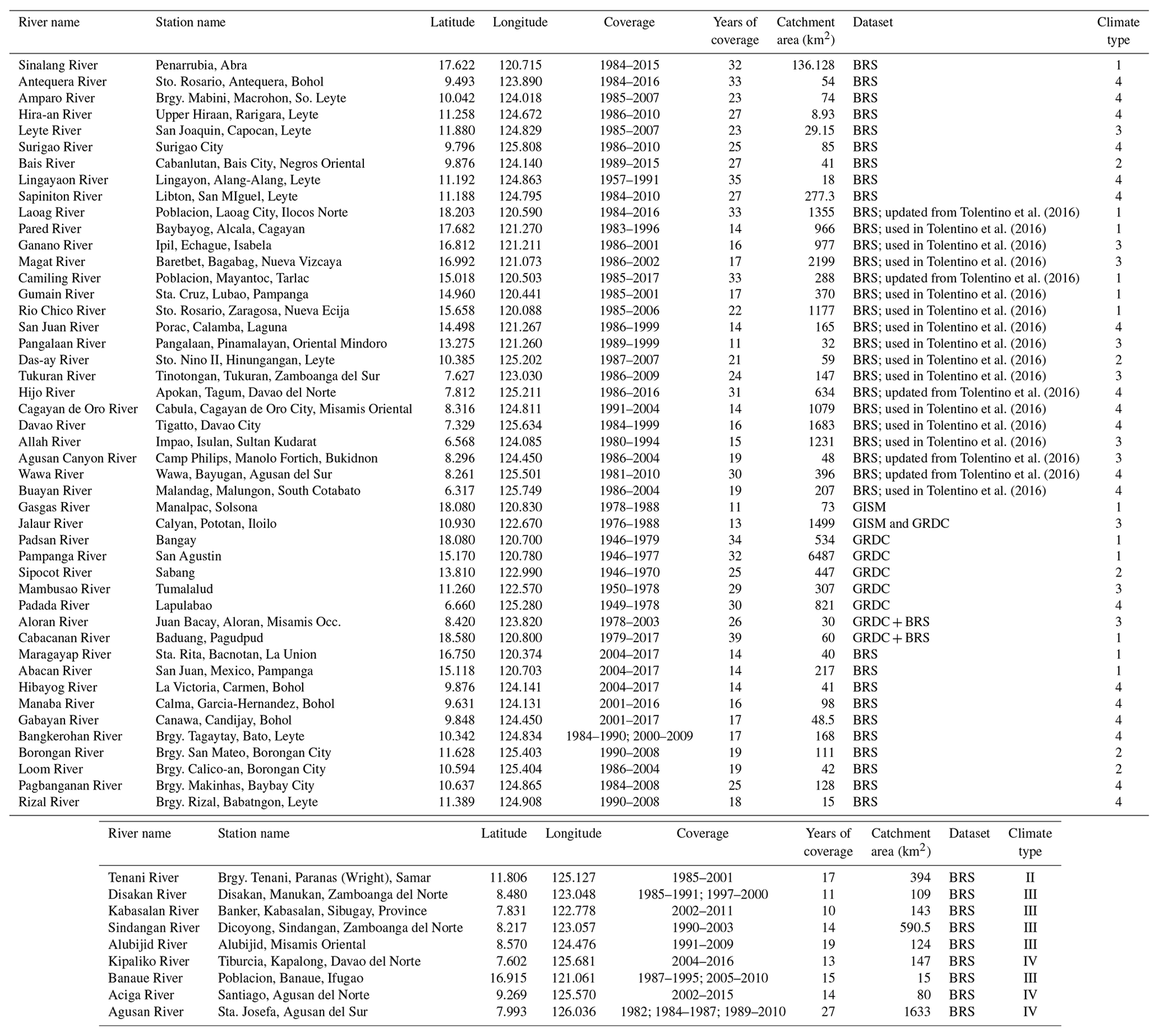
In this contribution we analyze monthly observations of discharge from 55 manually observed streamflow stations from three Philippine datasets. The observations span the period between 1946 to 2016, although only data through 2014 are used due to the time period included in GRUN (see Sect. 2.3). All datasets needed to include at least 10 years of data. The locations of all streamflow stations are shown in Fig. 1 and listed in Table 1.
Table 1List of stations used in this analysis including full station names, updated catchment areas, years of coverage, division and climate type.
2.2.1 Bureau of Research and Standards (BRS) dataset
The discharge data were originally acquired from the Bureau of Research Standards (BRS) under the Department of Public Works and Highways (DPWH). The record-keeping was transferred to the Bureau of Design, also under DPWH, which continues to record gauge data from some rivers up to today. The majority of the reprocessed BRS data used in this analysis come from Tolentino et al. (2016); some of the datasets were updated using data available from the Department of Public Works and Highways. A discussion of the accuracy of this data based on comparison to manual daily discharge measurements can be found in Tolentino et al. (2016).
2.2.2 Global Runoff Data Centre (GRDC) reference dataset
Data from 10 catchments from the GRDC reference dataset (https://www.bafg.de/GRDC/EN/04_spcldtbss/43_GRfN/refDataset_node.html; last access: July 2019) were analyzed. Over 45 sites from the Philippines are available in the GRDC data; however, almost none fulfilled our criteria of having over 10 years of data. Four of these catchments match or extended the BRS datasets, and one extends a GSIM dataset (see below). Notably four of the time series available from GRDC are available back to the 1940s (Table 1).
2.2.3 Global Streamflow Indices and Metadata archive (GSIM) reference dataset
Only two of the available five GSIM time series for the Philippines (Gudmundsson et al., 2018; Do et al., 2018) contain more than 10 years of data.
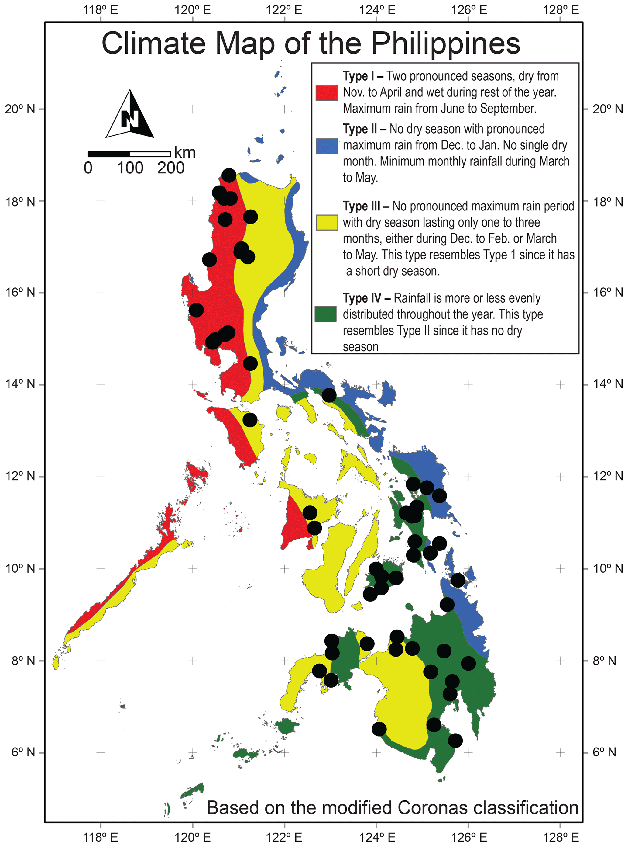
Figure 1Map of Philippines with the locations of streamflow stations used in this analysis and climatic type (as in Tolentino et al., 2016; Kintanar, 1984; Jose and Cruz, 1999).
2.3 GRUN observation-based global gridded () runoff dataset
GRUN is a recently published global reconstruction of monthly runoff time series for the period 1902 to 2014. It was created using a machine-learning algorithm based on temperature and precipitation data from the Global Soil Wetness Project Phase 3 (GSWP3; Kim et al., 2017; http://hydro.iis.u-tokyo.ac.jp/GSWP3/index.html, last access: December 2019) using the Global Streamflow Indices and Metadata Archive (GISM) (Ghiggi et al., 2019). In this contribution we analyzed GRUN v1 (https://figshare.com/articles/GRUN_Global_Runoff_Reconstruction/9228176; last access: 9 September 2019), which was trained on a selection of catchments with an area between 10 and 2500 km2 GSIM (Do et al., 2018; Gudmundsson et al., 2018) and validated using 379 large (>50 000 km2) monthly river discharge datasets from the Global Runoff Data Centre (GRDC) Reference Dataset (https://www.bafg.de/GRDC/EN/04_spcldtbss/43_GRfN/refDataset_node.html, last access: December 2019). Additionally, due to the criteria for training data, GRUN's calibration is biased towards the Northern Hemisphere midlatitudes; discharge data are available for only a few sites in the tropics in Africa and southeast Asia (Mulligan, 2013). Ghiggi et al. (2019) discuss that because of the dataset training technique, uncertainty scales with the magnitude of runoff. GRUN is likely to have high prediction uncertainty in regions with less-dense runoff observations and high discharge such as in tropical southeast Asia. However, Ghiggi et al. (2019) show for southeast Asia an increase in runoff and a strong correlation of runoff with ENSO for the period of analysis (1902 to 2014). We refer the reader to Ghiggi et al. (2019) for more information, but we note that because of the catchment size filtering criteria none of the GISM and GRDC data from the Philippines were used in calibration or evaluation (Gionata Ghiggi, personal communication, 2019). As such, we view our analysis as a completely independent test of the GRUN runoff prediction for small tropical catchments.
2.4 Catchment area and pairing with GRUN grid cells
All catchment areas were verified using the digital elevation model from the 2013 Interferometric Synthetic Aperture Radar (IfSAR) data. All runoff datasets were normalized (mm yr−1), i.e., “specific discharge”. We only considered streamflow stations where the published and verified areas agreed. Catchment areas span 4 orders of magnitude (8.93 to 6.487 km2) and cover the majority of the Philippines excluding Palawan (see Fig. 1). The location of catchments was paired to GRUN grid cells (0.5∘ by 0.5∘) for the analysis. Instead of computing the weighted area runoff over the catchment, we employed the nearest-neighbor interpolation between the catchment outlet location and the GRUN gridded product (0.5∘ by 0.5∘ resolution). All but one catchment is smaller than the area of the GRUN grid cells (∼2.500 km2); thus, we view this pairing as sufficient for validation purposes. This assumption was tested by interpolating the GRUN grid to the gauging location as well as the watershed centroids, but this did not lead to a significant difference in correlation.
2.5 Comparison of GRUN estimates and observations
To assess the performance of GRUN, we use a suite of metrics commonly used to assess model performance in hydrologic studies. Given the emphasis on a country-scale evaluation of GRUN, we primarily focus below on results in aggregate grouped by climate type or for all catchments. These metrics are calculated for each individual catchment (n=55) and in aggregate for each climate type (n=4; see below) shown in Fig. 1. GRUN was not intended to be used for estimating discharge for single small catchments; therefore, we focus on the aggregated data but also report the range for the result for the individual catchments.
Firstly, we use the commonly used coefficient of determination (r2 or r-squared values). This bivariate correlation metric measures the linear correlation between two variables: in this case the predicted monthly values from GRUN and the observed monthly values from the streamflow datasets. It varies from 0 (no linear correlation) to 1 (perfect correlation). The use of r squared does not account for systematic over- or underprediction in runoff, because it only accounts for correlation among the observed and predicted values (see Krause et al. (2005) for further discussion of the use of r squared in hydrological model assessment).
The second metric used here is the volumetric efficiency (VE) (Criss and Winston, 2008), utilized previously by Tolentino et al. (2016) on a subset of the BRS catchments analyzed here. VE is defined as
where Q is the monthly discharge, subscript P is used for the modeled or predicted values, and O is the observed runoff values. A value of 1 indicates a perfect score. Because we are interested in the performance of GRUN over the period of each streamflow record, we calculate VE using all paired monthly observed and simulated values rather than the monthly medians that were used in Tolentino et al. (2016). This results in lower VE scores than those reported by Tolentino et al. (2016).
Further, we use the linear Nash–Sutcliffe efficiency (NSE) (Nash and Sutcliffe, 1970):
The NSE can vary between −∞ and 1 (perfect fit). NSE values are useful, because values less than zero indicate that the model is no better than using the mean value of the observed data as a predictor. The logged NSE was also calculated using logarithmic values of runoff to reduce the influence of a mismatch during peak flow and to increase the influence of low-flow values (see further discussion in Krause et al., 2005).
To evaluate a possible strategy for performing a bias correction of the GRUN simulated values at a countrywide scale, we use the root mean square error (RMSE) in units of runoff (i.e., mm d−1). The RMSE was applied to the raw GRUN simulated values and the observation-based bias-corrected GRUN values at the country, climate type (see below), and individual catchment level.
Finally, to evaluate distributions of flow duration using flow duration curves by catchment and aggregated by climate type, we use the “fdc” function in the R package “hydroTSM” (Zambrano-Bigiarini, 2020), and we include in our comparison GRUN-predicted values only for months which observations are available.
Figure 2 and the supplemental figures (Fig. S1 in the Supplement) show comparisons between the time series of the GRUN runoff values and runoff (area normalized discharge). Statistics performance metrics across all data as well as by climate types I to IV are listed in Tables 2 and S1 (in the Supplement). In the following sections, we break down the comparison between the streamflow observations and GRUN by reporting summary statistics, comparing runoff distributions and extreme values at the individual basin level as well as by climate type, analyze flow duration curves, and finally look at several correlations of VE to watershed characteristics. Following this we calculate bias correction regressions and provide an outlook for future work.

Figure 2Example time series of GRUN-predicted (red lines) and observed (black lines) runoff values, and cross plots (log scale) with VE, r2, and RMSE values for the worst (a, b) and best (c, d) performing river basins within climate types I, II, III, and IV (panels a–d, respectively).
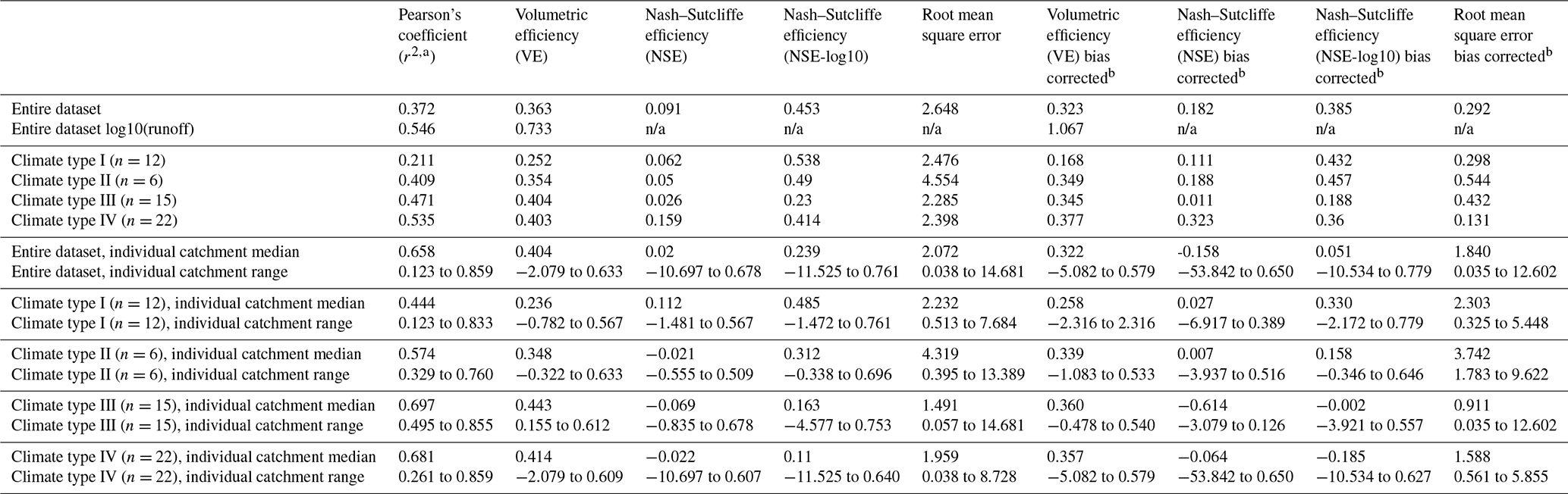
Table 2Results of statistical agreement between GRUN aggregated by climate type and for the entire dataset (see Table S1 for individual catchments). Median monthly runoff values are 5.29, 9.03, 4.99, and 5.51 mm d−1 for climate types I–IV, respectively.
a for regressions forced through intercept of 0. b two-step bias correction procedure where first mean offset is added to the predicted GRUN values and then a log-transform stretch correction is applied (see text for details). n/a stands for not applicable.
3.1 Comparison of runoff distributions
Average runoff values among all catchments are somewhat well predicted by GRUN. Across all observations the r squared of the correlation between GRUN prediction and observation was 0.372, and VE was 0.363 (Table 2). Using log(runoff) values (following Criss and Winston, 2008), the r squared improved to 0.546 and a VE to 0.733, suggesting reasonable utility in the GRUN product at the country scale for the Philippines, even though no training data from the Philippines were used in the creation of GRUN. The RMSE across the dataset was 2.648 mm d−1 (Table 2). NSE and NSE-log10 values ranged from −10.70 to 0.68 and from −11.53 to 0.76, for individual catchment comparisons, with median values of 0.02 and 0.24, respectively. For more than half of the catchments (29 of 55), NSE values were greater than 0, but for only five catchments it was higher than 0.5. Similarly, for 32 of 55 catchments the NSE-log10 values were greater than 0 and for 12 catchments greater than 0.5.
The VE of the median values of runoff (black dots in Fig. 3a) was 0.509 across all catchments; the average (mean) difference between the observed and simulated median runoff values was +16 % (Fig. 3a). The median and interquartile ranges (IQRs, 25 % to 75 %) of the runoff for the individual catchments for the GRUN and the observations overlap (Fig. 2e). For two large catchments and three relatively small catchments, the IQR of the observations does not overlap with the GRUN runoff IQR. The three small catchments are located in climate type III (yellow) and the two large catchments are climate type IV. For two catchments of moderate size, the GRUN IQR is greater than the observed IQR runoff range.

Figure 3Comparison of runoff ranges and distributions. (a) Comparison of median and extreme (maximum and minimum) monthly runoff for the observations and GRUN in log space. (b–d) As in (a) for the minimum, median, and maximum monthly values, respectively, in linear space. (e) Distribution of runoff – observations (colored) and GRUN (white) – for the individual catchments (ordered by size). Plots show the median (line), interquartile range (box), and maximum and minimum values (whiskers). The boxplots for GRUN also only include months for which observations are available.
Looking at extreme monthly values (maximum and minimum) over the period of observation demonstrates significant underprediction during the wettest conditions (orange dots in Fig. 3a and d). For almost all catchments, the maximum observations plot above the 1:1 line. The VE for the maximum runoff is lower than for the median runoff (0.194). The minimum values plot around the 1:1 line and are more evenly distributed; however, the VE score for the minimum runoff (0.154) is similarly low due to greater spread than for the median values.
Regardless of climate type, a general underestimation of the model is seen for the highest runoff, but this is especially evident for catchments in climate types I and II with pronounced wet seasons (as also shown by their lower r-squared values; Fig. 4) and lower VE values. For climate type II, the RMSE value of 4.55 mm d−1 (compared to an average observed flow of 9.03 mm d−1) is also the highest. Climate types III and IV have comparable r-squared and VE values and skewness towards underprediction during the highest runoff months is still evident, particularly for climate type IV. These patterns are particularly evident looking at Fig. 5, which shows flow duration curves (FDC) by climate type for individual catchments groups (see Fig. S2 for individual catchment comparisons). Such an analysis allows for inspection of runoff distributions and biases across the range of observed and predicted values. At low flows (high exceedance probability, >80 %) there is reasonable agreement in the shape and magnitude of the distributions between GRUN and the observations for climate types I and IV (bottom right of the FDC plots). For climate type III, there is a consistent bias across all runoff values with an exceedance probability < 90 %. At high flow (low exceedance probability < 20 %), as also noted above, runoff for all climate types is underestimated by GRUN, with the greatest discrepancy for climate types I and II (top left of each FDC plot).
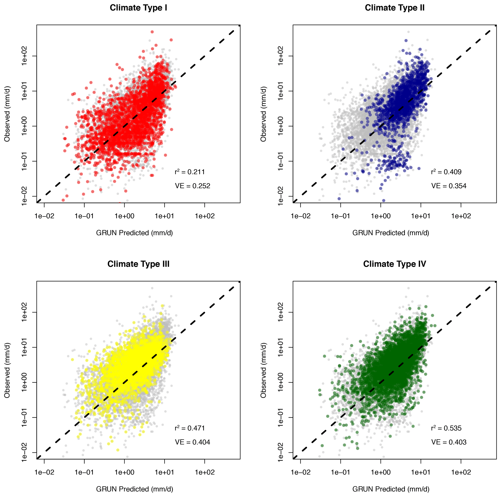
Figure 4Plots of GRUN-predicted vs. observed monthly runoff by climate type (see Fig. 1 for climate type distributions). Grey dots represent all data; colored dots represent data points from the particular climate type. The squared Pearson correlation coefficient (r2) and volumetric efficiency (VE) metrics are listed for each panel.
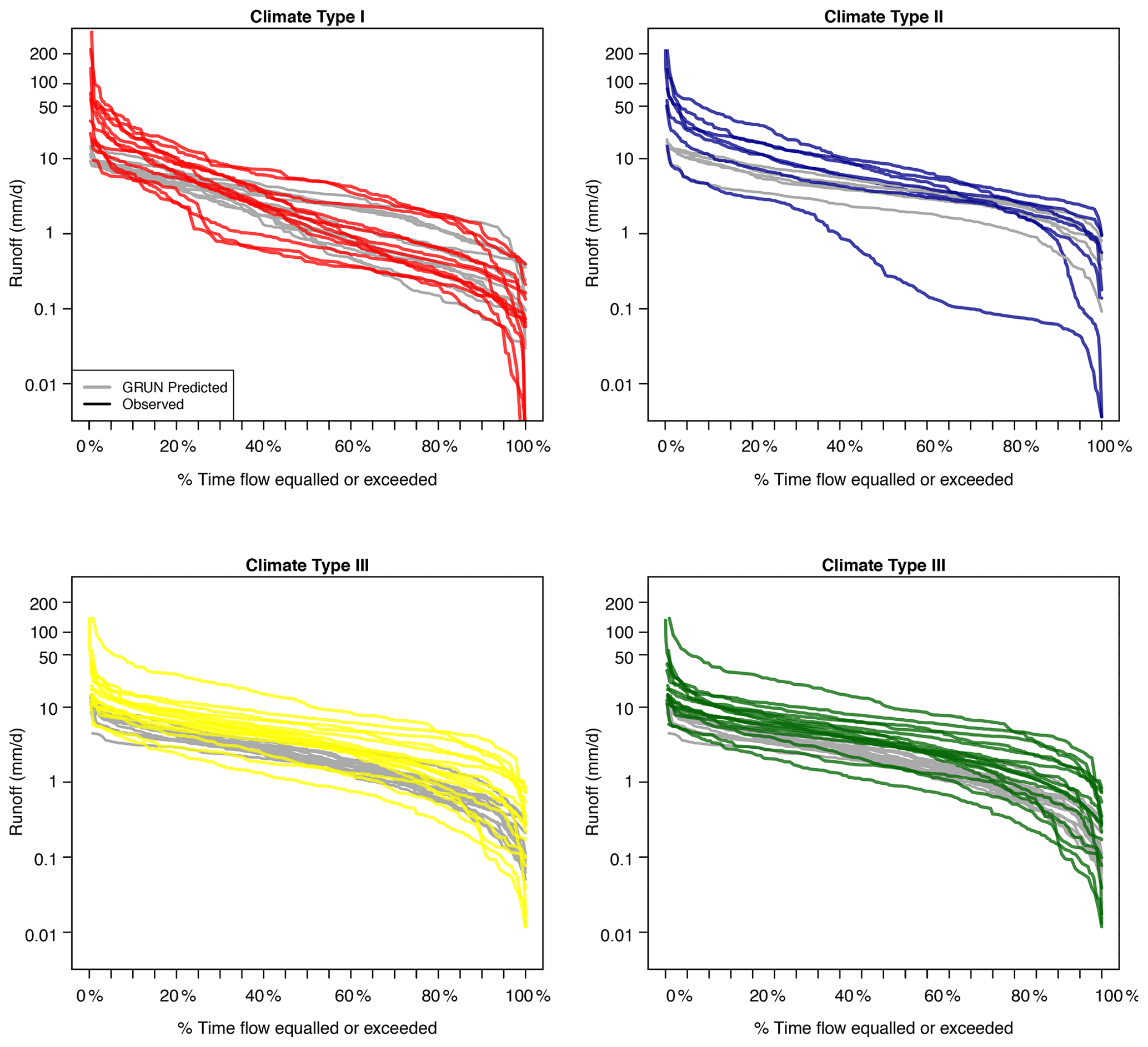
Figure 5Flow Duration Curves (FDC) of individual catchments by climate type. For each climate type, the observed (colored) and GRUN-predicted (grey) runoff distributions are shown for each catchment. These plots represent the rank ordered data shown in Fig. 4. FDC comparisons for each individual catchments are compiled in Fig. S2.
3.2 Correlation and trends with watershed characteristics
The biases noted above are likely due to the high uncertainty and underprediction in monsoonal precipitation that is used for input into GRUN. There is a significant negative correlation (at p<0.01, r2=0.391) between log values of maximum runoff difference (observed minus predicted) and catchment area (not shown). This suggests two possibilities: first, that, particularly for small catchments which may have steeper average slope, GRUN underpredicts monthly runoff values during the wet season due to the bias in the precipitation datasets used to create GRUN and second that model–data agreement improves with catchment size. In this section we explore these possibilities.
There was a weak positive correlation (r2=0.041, p=0.137) between VE and log(catchment size) (Fig. 6) and a stronger negative correlation with mean runoff (r2=0.182, p<0.01). However, for catchments with a low mean runoff there is significant spread in VE score, driven primarily by climate type I catchments (red box and whisker plot in Fig. 6c). These catchments experience distinct wet and dry seasons and are predominantly located in the northwest Philippines. The positive correlation with catchment size is likely primarily due to the extreme wet months. The bias of the GRUN data at high and moderate flow conditions is particularly evident in the flow duration curves (Fig. 5). This is also more in line with the Nash–Sutcliffe efficiency (NSE) compared to the log(Nash–Sutcliffe efficiency) (NSE-log10) scores (Tables 2 and S1), because NSE puts more weight on high flow (Criss and Winston, 2008) as well as the higher VE scores for log10 runoff values for all the runoff data across the entire dataset (0.363 vs. 0.733; Table 2). The physical significance of these results could be that for large basins the time of concentration of any given flood event will be much longer; thus, flood peaks will be wider and subdued due to infiltration into the shallow aquifers. However, a more likely explanation is that the average rainfall intensity is too low in the GSWP3 precipitation data used in producing GRUN. This is likely due to downscaling from averages over larger areas with topographic complexity. While GSWP3 uses downscaled 20th century reanalysis products (Kim et al., 2017) at T248 resolution (∼0.5∘, the same resolution as GRUN), the topographic complexity of tropical islands such as the Philippines on the sub-0.5∘ scale would likely result in smoothing of the variability and lowering of the absolute magnitude of the precipitation fields, particularly for small catchments and during the wet season and during large synoptic precipitation events during the monsoon season. Finally, while the GSWP3 precipitation inputs are bias-corrected using the Global Precipitation Climatology Centre precipitation network, previous work has highlighted data quality issues with some historical data from the Philippines (Schneider et al., 2014).

Figure 6Diagnostic plots of volumetric efficiency (VE) results and comparison across metrics. Cross plots show the correlation of VE with (a) catchment area and (b) mean runoff. (c) Box and whisker plots show data from distribution of VE by climate type. Box and whisker plots show the median, interquartile range and 95 % confidence intervals and outliers (dots). The regression in (a) is between the VE scores and ln(Catchment Area). (d–f) As in (c) for r2, NSE, and NSE-log10.
The underestimation of runoff values during extreme rain events is most likely due to an underestimation in the wet season rainfall products from GSWP3 used to create GRUN as described above. Alternatively, it may be a result of the fast saturation of the overlying soil and shallow aquifers filling up during the wet season, as well as potentially high amounts of direct runoff (e.g., Tarasova et al., 2018). On the other hand, the underestimation of flow during low-flow events may be a result of not accurately accounting for stream baseflow which is fed by shallow aquifers and influenced by land use and surface properties. These effects may be buffered in larger catchments, leading to the increase in that model–data agreement with catchment size (Fig. 6b).
Previous studies have investigated the correlation between runoff and catchment size (Mayor et al., 2010) and the different hydrologic and geologic factors that cause nonlinear relationships between these two variables (Rodríguez-Caballero et al., 2014). Recently, Zhang et al. (2019) point out that runoff coefficients increase logarithmically as catchment size decreases. Moreover, the same study reports that the effects of vegetation cover, slope, and land use are larger for smaller catchments than for larger catchments. This implies that prediction of basin runoff for smaller catchments is more difficult due to the variations in the compounding factors mentioned above. We hypothesize that the effects proposed by Zhang et al. (2019) also influence the Philippines streamflow dataset used in this study.
3.3 Bias correction and outlook
Overall, GRUN underestimates the actual observed runoff for the Philippine basins. The GRUN dataset predicts a range of 0 to 10 mm d−1 for most basins and up to 20 mm d−1 for larger basins. The observed maximum monthly runoff values are on average higher and exceed 50 mm d−1 during months with extreme rain events (Fig. 4). The bias is largest for the high flows (Figs. 3a and 5). Furthermore, the GRUN dataset also appears to underestimate minimum flow in streams from highly seasonal catchments (e.g., types I and II).
Given the biases and in particular the clear underprediction of streamflow in GRUN during the wettest months, we perform a bias correction of the GRUN dataset at a nationwide level using all the available data used in our analysis. We do so in a two-step process to both correct the mean offset and stretch the wettest months to higher values with all transformations occurring in log-transform space (i.e., as displayed in cross plots in Figs. 2 and 4). Thus, we first add the mean log10(runoff) difference between the observations and the predicted values (0.117±0.045). Following this, using the lm function in R, we fit a linear regression between the observations and the GRUN-predicted values (log10(runoff, observed) = m × log10(runoff, predicted) + b) and correct the predicted values using the slope () and intercept () derived from this regression. Uncertainties reported here are 68 % confidence intervals and were assessed by bootstrap resampling observation and prediction pairs from 20 catchments (vertical line in Fig. 7) without replacement 10 000 times. In Fig. 7 we show the influence of including an increasing number of catchments from the dataset in our bootstrap resampling to assess how the mean value of the coefficients asymptotically converge as more catchments are included. While the mean log10(runoff) offset is relatively unaffected, the slope and intercept of the bias correction do not reach a stable number until more than 10 catchments are included in the analysis. A leave-one-out approach (i.e., calculating the coefficients with 54 of 55 catchments) indicates 68 % confidence uncertainties of ±0.005, ±0.006, and ±0.003 for the log10(runoff) offset, the slope, and intercept, which are lower than those reported above, as expected.
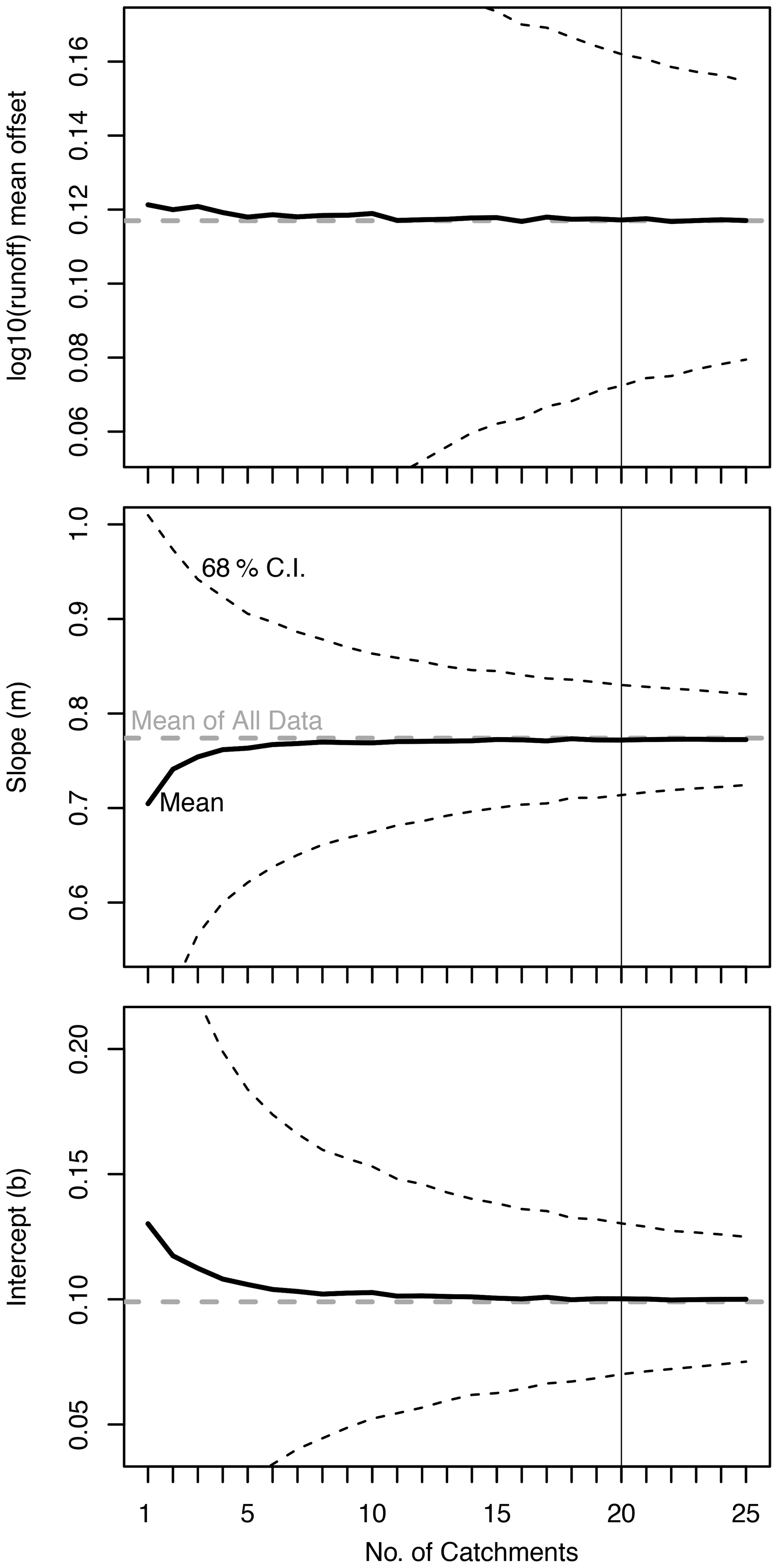
Figure 7Bootstrap uncertainty of bias correction. Plotted vs. the number of catchments is the mean and confidence interval (68 %) log10(runoff) offset, the slope, and intercept of the bias correction determined via random sampling at the catchment level without replacement. The vertical line at 20 catchments is the uncertainty reported in the text where all three coefficients asymptotically converge to the mean values determined using the entire dataset.
By carrying out these calculations in log-transform space the highest GRUN runoff values are the most affected, which are the data points that were most underpredicted (Figs. 3a and 4). Because these corrections were carried out in log10 space statistical bias in the form of underestimation is possible (Ferguson, 1986). Following Ferguson (1986) we calculated the unbiased estimate of the variance (notated as “s”) as 0.0686 mm d−1 which gives a correction factor (calculated as exp(2.65 s2) of 1.0126. This correction factor, a multiplier, can be applied to the bias corrected values to adjust for possible the bias due to the log10 space regression we have implemented.
To assess this bias correction, we calculated RMSE values at a catchment, climate type, and countrywide level (Fig. 8 and Tables 2 and S1). The log-transform bias correction improves the nationwide RMSE value by an order of magnitude (2.648 vs. 0.292) and most significantly improves catchments in climate types III and IV (Fig. 8; 2.285 vs. 0.432 and 2.398 vs. 0.131, respectively; Table 2). Interestingly, the median RMSE value for climate type I and II catchments was not notably improved; however, the RMSE range for both was reduced (red and blue boxes in Fig. 8, respectively).
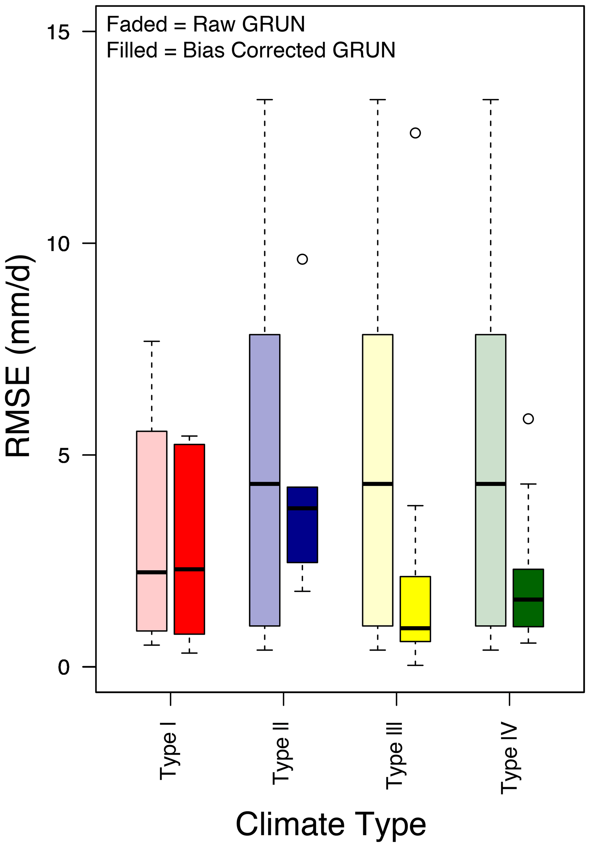
Figure 8Box and whisker plots of the root mean square error (RMSE) for catchments grouped by climate type of observed values versus raw GRUN values (light-colored boxes) and bias-corrected GRUN values (dark-colored boxes). For bias correction equation and country-wide results, see Table 2.
This analysis and the improvement of RMSE values, as well as some of performance metrics such as NSE (see scores tabulated in Table 2), using a simple log-transform-based bias correction demonstrates the importance of either (1) including smaller catchments in future products such as GRUN or (2) performing similar bias corrections on a country, region or even catchment scale as needed. This is particularly important because if taken at face value the proportional contribution of relatively small tropical land areas to global discharge (e.g., Dai and Trenberth, 2002) would be underestimated without such corrections.
Based on monthly runoff observations from catchments in the Philippines with more than 10 years of data between 1946 and 2014, there is a significant but weak correlation (r2=0.372) between the GRUN-predicted runoff values and actual observations. The results indicate a somewhat skillful prediction for monthly runoff (volumetric efficiency = 0.363 and log(Nash–Sutcliffe efficiency) = 0.453) when all data are pooled. Looking at different hydrometeorological regimes, we demonstrated that GRUN performs better for low rainfall catchments located in climate types III and IV. There was a weak negative positive correlation between volumetric efficiency and catchment area. Further, we found that, particularly for smaller catchments, maximum wet season runoff values are grossly underpredicted by GRUN. The application of a nationwide bias correction to stretch high runoff values using log-transformed runoff values greatly improved the RMSE of the predicted values. Global databases such as GRUN can be applicable for aggregated stream discharge estimates and to investigate general trends in the hydrologic characteristics of a region (such as in previous work, e.g., Merz et al., 2011; Wanders and Wada, 2015), but bias correction is needed when applying them to smaller catchments or regions for which data were not used in the development of the dataset. GRUN was not intended to be used for estimating discharge for single small catchments; however, it is applicable for use in regional and country-scale analyses provided that proper statistical comparisons of modeled versus actual gauged data are performed. The recommended bias correction presented here will likely improve such estimates and analyses for the Philippines. We thus propose that the use of the GRUN dataset can be extended to other ungauged tropical regions with smaller catchments after at least applying a similar correction as described in this study.
Data were compiled from the DPWH-BRS, GISM, and GRDC datasets (see links in text) and are made available as a Supplement. The supplemental file “PhilippinesRiverDischarge_Ibarra_HESS.xlsx” contains individual tabs for each catchment in the same order as Figs. S1 and S2. The runoff time series start with January of the first year that data are available. Blank cells indicate no measurement. The first three rows include the major river basin, the river name, and the location of the station. Further metadata including location (latitude and longitude), area, and data source can be found in Table S1.
The supplement related to this article is available online at: https://doi.org/10.5194/hess-25-2805-2021-supplement.
DEI and CPCD designed the study, DEI and PLMT carried out the dataset compilation and screening, PLMT verified catchment areas, DEI and PLMT carried out the analysis, and DEI and CPCD prepared the article with contributions from PLMT.
The authors declare that they have no conflict of interest.
We thank the Republic of the Philippines Department of Science and Technology Philippine Council for Industry, Energy, and Emerging Technology Research and Development (DOST-PCIEERD) Balik Scientist program for facilitating collaboration between the authors in 2019. We acknowledge the help of Mart Geronia, Allen Marvin Yutuc, Iris Joy Gonzales, Jia Domingo, and Eduardo J. Terciano Jr. for help with dataset compilation, as well as Tyler Kukla for discussing the statistical methods. We thank DPWH-BRS, GISM, and GRDC for datasets availability. Finally, we thank Jaivime Evaristo and an anonymous referee for thorough and helpful reviews and edits; the editor, Wouter Buytaert, for handling our paper; and Gionata Ghiggi for ensuring accurate representation of the GRUN product and comments on the article.
This project was partially supported through the DOST-PCIEERD project entitled, Catchment Susceptibility to Hydrometeorological Events supporting Tolentino and David, and a DOST-PCIEERD Balik Scientist award to Ibarra. Ibarra is funded by the UC Berkeley Miller Institute and UC President's Postdoctoral Fellowship.
This paper was edited by Wouter Buytaert and reviewed by Jaivime Evaristo and one anonymous referee.
Abon, C. C., David, C. P. C., and Bellejera, N. E. B.: Reconstructing the Tropical Storm Ketsana flood event in Marikina River, Philippines, Hydrol. Earth Syst. Sci., 15, 1283–1289, https://doi.org/10.5194/hess-15-1283-2011, 2011.
Abon, C. C., Kneis, D., Crisologo, I., Bronstert, A., David, C. P. C., and Heistermann, M.; Evaluating the potential of radar-based rainfall estimates for streamflow and flood simulations in the Philippines, Geomat. Nat. Haz. Risk., 7, 1390–1405, https://doi.org/10.1080/19475705.2015.1058862, 2016.
Alfieri, L., Lorini, V., Hirpa, F. A., Harrigan, S., Zsoter, E., Prudhomme, C., and Salamon, P.: A global streamflow reanalysis for 1980–2018, J. Hydrol., 6, 100049, https://doi.org/10.1016/j.hydroa.2019.100049, 2020.
Criss, R. E. and Winston, W. E.: Do Nash values have value? Discussion and alternate proposals, Hydrol. Process., 22, 2723–2725, https://doi.org/10.1002/hyp.7072, 2008.
Dai, A. and Trenberth, K. E.: Estimates of Freshwater Discharge from Conntinents: Latitudinal and Seasonal Variations, J. Hydrometeorol., 3, 660–687, 2002.
David, C. P., Cruz, R. V. O., Pulhin, J. M., and Uy, N. M.: Freshwater Resources and Their Management, in: Philippine Climate Change Assessment Report WG2: Impacts, Vulnerabilities and Adaptation, OML Foundation, Pasig, Philippine, 34–54, 2017.
Davie, J. C., Falloon, P. D., Kahana, R., Dankers, R., Betts, R., Portmann, F. T., Wisser, D., Clark, D. B., Ito, A., Masaki, Y., and Nishina, K.: Comparing projections of future changes in runoff from hydrological and biome models in ISI-MIP, Earth Syst. Dynam., 4, 359–374, https://doi.org/10.5194/esd-4-359-2013, 2013.
Do, H. X., Gudmundsson, L., Leonard, M., and Westra, S.: The Global Streamflow Indices and Metadata Archive (GSIM) – Part 1: The production of a daily streamflow archive and metadata, Earth Syst. Sci. Data, 10, 765–785, https://doi.org/10.5194/essd-10-765-2018, 2018.
Evaristo, J. and McDonnell, J. J.: Global analysis of streamflow response to forest management, Nature, 570, 455–461, https://doi.org/10.1038/s41586-019-1306-0, 2019.
Ferguson, R. I.: River Loads Underestimated by Rating Curves, Water Resour. Res., 22, 74–76, https://doi.org/10.1029/WR022i001p00074, 1986.
Ghiggi, G., Humphrey, V., Seneviratne, S. I., and Gudmundsson, L.: GRUN: An observations-based global gridded runoff dataset from 1902 to 2014, Earth Syst. Sci. Data, 11, 1655–1674, https://doi.org/10.5194/essd-11-1655-2019, 2019.
Gudmundsson, L., Do, H. X., Leonard, M., and Westra, S.: The Global Streamflow Indices and Metadata Archive (GSIM) – Part 2: Quality control, time-series indices and homogeneity assessment, Earth Syst. Sci. Data, 10, 787–804, https://doi.org/10.5194/essd-10-787-2018, 2018.
Hagemann, S., Chen C., Haerter, J. O., Heinke, J., Gerten, D., and Piani, C.: Impact of a Statistical Bias Correction on the Projected Hydrological Changes Obtained from Three GCMs and Two Hydrology Models, J. Hydrometerol., 12, 556–578, https://doi.org/10.1175/2011JHM1336.1, 2011.
Harrigan, S., Zsoter, E., Alfieri, L., Prudhomme, C., Salamon, P., Wetterhall, F., Barnard, C., Cloke, H., and Pappenberger, F.: GloFAS-ERA5 operational global river discharge reanalysis 1979–present, Earth Syst. Sci. Data, 12, 2043–2060, https://doi.org/10.5194/essd-12-2043-2020, 2020.
Jose, A. M. and Cruz, N. A.: Climate change impacts and responses in the Philippines: water resources, Clim. Res., 12, 77–84, 1999.
Kim, H., Watanabe, S., Chang, E. C., Yoshimura, K., Hirabayashi, J., Famiglietti, J., and Oki, T.: Global Soil Wetness Project Phase 3 Atmospheric Boundary Conditions (Experiment 1) [Data set], Data Integration and Analysis System (DIAS), https://doi.org/10.20783/DIAS.501, 2017.
Kintanar, R. L.: Climate of the Philippines, PAGASA report, Philippine Atmospheric, Geophysical and Astronomical Services Administration, Quezon City, Philippines, 38 pp., 1984.
Krause, P., Boyle, D. P., and Bäse, F.: Comparison of different efficiency criteria for hydrological model assessment, Adv. Geosci., 5, 89–97, https://doi.org/10.5194/adgeo-5-89-2005, 2005.
Kumar, P., Masago, Y., Mishra, B. K., and Fukushi, K., Evaluating future stress due to combined effects of climate change and rapid urbanization for Pasig Marikina river, Manila, Groundwater Sustain. Dev., 6, 227–234, https://doi.org/10.1016/j.gsd.2018.01.004, 2018.
Kummu, M., Guillaume, J. H. A., de Moel, H., Eisner, S., Flörke, M., Porkka, M., Siebert, S., Veldkamp, T. I. E., and Ward, P. J.: The world's road to water scarcity: shortage and stress in the 20th century and pathways towards sustainability, Nat. Sci. Rep., 6, 38495, https://doi.org/10.1038/srep38495, 2016.
Mayor, A. G., Bautista, S., and Bellot, J.: Scale-dependent variation in runoff and sediment yield in a semiarid Mediterranean catchment, J. Hydrol., 397, 128–135, 2010.
Merz, R., Parajka, J., and Bloschl, G.: Time stability of catchment model parameters: Implications for climate impact analyses, Water Resour. Res., 47, W02531, https://doi.org/10.1029/2010WR009505, 2011.
Meybeck, M., Kummu, M., and Dürr, H. H.: Global hydrobelts and hydroregions: improved reporting scale for water-related issues, Hydrol. Earth Syst. Sci., 17, 1093–1111, https://doi.org/10.5194/hess-17-1093-2013, 2013.
Mulligan, M.: WaterWorld: a self-parameterising, physically based model for application in data-poor but problem-rich environments globally, Hydrol. Res., 44, 748–769, https://doi.org/10.2166/nh.2012.217, 2013.
Nash, J. E. and Sutcliffe, J. V.: River flow forecasting through conceptual models part I – A discussion of principles, J. Hydrol., 10, 282–290, https://doi.org/10.1016/0022-1694(70)90255-6, 1970.
Nurse, L. A., McLean, R. F., Agard, J., Briguglio, L. P., Duvat-Magnan, V., Pelesikoti, N., Tompkins, E., and Webb, A.: Small islands, in: Climate Change 2014: Impacts, Adaptation, and Vulnerability, Part B: Regional Aspects, Contribution of Working Group II to the Fifth Assessment Report of the Intergovernmental Panel on Climate Change, chap. 29, edtited by: Barros, V. R., Field, C. B., Dokken, D. J., Mastrandrea, M. D., Mach, K. J., Bilir, T. E., Chatterjee, M., Ebi, K. L., Estrada, Y. O., Genova, R. C., Girma, B., Kissel, E. S., Levy, A. N., MacCracken, S., Mastrandrea, P. R., and White, L. L., Cambridge University Press, Cambridge, UK and New York, NY, USA, 1613–1654, 2014.
Paronda, G. R. A., David, C. P. C., and Apodaca, D. C.: River flow patterns and heavy metals concentrations in Pasig River, Philippines as affected by varying seasons and astronomical tides, IOP Conf. Ser.: Earth Environ. Sci., 344, 012049, https://doi.org/10.1088/1755-1315/344/1/012049, 2019.
Rodríguez-Caballero, E., Cantón, Y., Lazaro, R., and Sole-Benet, A.: Cross-scale interactions between surface components and rainfall properties. Non-linearities in the hydrological and erosive behavior of semiarid catchments, J. Hydrol., 517, 815–825, https://doi.org/10.1016/j.jhydrol.2014.06.018, 2014.
Schneider, U., Becker, A., Finger, P., Meyer-Christoffer, A., Ziese, M., and Rudolf, B.: GPCC's new land surface precipitation climatology based on quality-controlled in situ data and its role in quantifying the global water cycle, Theor. Appl. Climatol., 115, 15–40, https://doi.org/10.1007/s00704-013-0860-x, 2014.
Tarasova, L., Basso, S., Zink, M., and Merz, R.: Exploring Controls on Rainfall-Runoff Events: 1. Time Series-Based Event Separation and Temporal Dynamics of Event Runoff Response in Germany, Water Resour. Res., 54, 7711–7732, https://doi.org/10.1029/2018WR022587, 2018.
Tolentino, P. L. M., poortinga, A., Kanamaru, H., Keesstra, S., Maroulis, J., David, C. P. C., and Ritsema, C. J.: Projected Impact of Climate Change on Hydrological Regimes in the Philippines, PLoS ONE, 11, e0163941, https://doi.org/10.1371/journal.pone.0163941, 2016.
Wanders, N. and Wada, Y.: Decadal predictability of river discharge with climate oscillations over the 20th and early 21st century, Geophys. Res. Lett., 42, 10689–10695, https://doi.org/10.1002/2015GL066929, 2015.
WEF: The Global Risks Report 2018, available at: http://reports.weforum.org/global-risks-2018/ (last access: December 2019), 2018.
Winsemius, H. C., Aerts, J. C., Van Beek, L. P., Bierkens, M. F., Bouwman, A., Jongman, B., Kwadijk, J. C., Ligtvoet, W., Lucas, P. L., Van Vuuren, D. P., and Ward, P. J.: Global drivers of future river flood risk, Nat. Clim. Change, 6, 381–385, https://doi.org/10.1038/nclimate2893, 2016.
Zambrano-Bigiarini, M.: Time Series Management, Analysis and Interpolation for Hydrological Modelling, CRAN [code], available at: https://cran.r-project.org/web/packages/hydroTSM/hydroTSM.pdf, last access: May 2020.
Zhang, Q., Liu, J., Yu, X., and chen, L.: Scale effects on runoff and a decomposition analysis of the main driving factors in the Haihe Basin mountainous area, Sci. Total Environ., 690, 1089–1099, https://doi.org/10.1016/j.scitotenv.2019.06.540, 2019.