The spatial extent of hydrological and landscape changes across the mountains and prairies of Canada in the Mackenzie and Nelson River basins based on data from a warm-season time window

East of the Continental Divide in the cold interior of Western Canada, the Mackenzie and Nelson River basins have some of the world's most extreme and variable climates, and the warming climate is changing the landscape, vegetation, cryosphere, and hydrology. Available data consist of streamflow records from a large number (395) of natural (unmanaged) gauged basins, where flow may be perennial or temporary, collected either year-round or during only the warm season, for a different series of years between 1910 and 2012. An annual warm-season time window where observations were available across all stations was used to classify (1) streamflow regime and (2) seasonal trend patterns. Streamflow trends were compared to changes in satellite Normalized Difference Indices.

Clustering using dynamic time warping, which overcomes differences in streamflow timing due to latitude or elevation, identified 12 regime types. Streamflow regime types exhibit a strong connection to location; there is a strong distinction between mountains and plains and associated with ecozones. Clustering of seasonal trends resulted in six trend patterns that also follow a distinct spatial organization. The trend patterns include one with decreasing streamflow, four with different patterns of increasing streamflow, and one without structure. The spatial patterns of trends in mean, minimum, and maximum of Normalized Difference Indices of water and snow (NDWI and NDSI) were similar to each other but different from Normalized Difference Index of vegetation (NDVI) trends. Regime types, trend patterns, and satellite indices trends each showed spatially coherent patterns separating the Canadian Rockies and other mountain ranges in the west from the poorly defined drainage basins in the east and north. Three specific areas of change were identified: (i) in the mountains and cold taiga-covered subarctic, streamflow and greenness were increasing while wetness and snowcover were decreasing, (ii) in the forested Boreal Plains, particularly in the mountainous west, streamflows and greenness were decreasing but wetness and snowcover were not changing, and (iii) in the semi-arid to sub-humid agricultural Prairies, three patterns of increasing streamflow and an increase in the wetness index were observed. The largest changes in streamflow occurred in the eastern Canadian Prairies.

1 Introduction

Western Canada, east of the Continental Divide, has extreme and variable climates and is experiencing rapid environmental change (DeBeer et al., 2016) where a changing climate is affecting the landscape, the vegetation, and the water. The southern part of this region sustains 80 % of Canada's agricultural production, a large portion of its forest wood, and pulp and paper production and also includes several globally important natural resources (e.g. uranium, potash, coal, petroleum). Understanding both observed changes and possible future changes is clearly in the national interest. Climate variation and change have been demonstrated to have important effects on the rivers of Canada (Whitfield and Cannon, 2000; Zhang et al., 2001; Whitfield et al., 2002; Janowicz, 2008; Déry et al., 2009a, b; Tan and Gan, 2015), including Western Canada's cold interior (Luckman, 1990; Burn, 1994; Luckman and Kavanaugh, 2000; Ireson et al., 2015; Dumanski et al., 2015; Ehsanzadeh et al., 2016). The sensitivity of streamflow to changes in temperature and precipitation may differ by period of the year (Leith and Whitfield, 1998; Whitfield and Cannon, 2000; Botter et al., 2013). Trends in water storage, based on Gravity Recovery and Climate Experiment (GRACE) satellites, identified precipitation increases in northern Canada, a progression from a dry to a wet period in the eastern Prairies/Great Plains, and an area of surface water drying in the eastern boreal forest (Rodell et al., 2018). The Mackenzie and Nelson (Saskatchewan and Assiniboine–Red) River basins were the focus of this study and are where cold-region climatic, hydrological, ecological, and cryospheric processes are highly susceptible to the effects of warming. Both rivers arise in the Canadian Rockies and receive the vast majority of their runoff from high-elevation headwater basins that are dominated by heavy snowfall, long-lasting seasonal snowcover, glaciers, and icefields. The whole region is subject to strong seasonality, continental climate, near absence of winter rainfall, and seasonally frozen soils. From the mid-boreal forest northwards and at high elevations, the surface is an annually thawed active layer below which materials are permanently frozen (permafrost). Tens of millions of lakes and wetlands cover the northern and eastern parts of this region, where the Canadian Shield dominates topography and hydrography. Cold winters and coincidence of the precipitation maximum with the snowmelt period or postmelt period mean that rivers and streams have minimum flows in late winter and maximum flows in late spring. This study provides a statistical assessment of patterns and recent changes in the warm-season hydrological regime and in satellite indices of vegetation, water storage, and snow and of the spatial patterns of these changes at gauged basins across this large domain.

Hydrological processes differ widely in this domain, which spans 11 of Canada's 15 terrestrial ecozones and includes many small basins where streamflow is only temporary (Buttle et al., 2012). The hydrographs of all rivers in this domain reflect contributions from snowmelt, the magnitudes of which differ in both space and time. Other flow contributions, from glaciers and rainfall, all vary spatially across the domain, with glacier contributions focussed in high mountain headwaters and rainfall contributions increasing at lower elevations and latitudes. Ecozones (Marshall et al., 1999; Eamer et al., 2014; Ireson et al., 2015) were chosen as an appropriate level for comparisons rather than physical attributes such as climate, permafrost, or geology, since ecozones represent regions where the ecology and physical environment operate as a system. It is important to note that many rivers in this study originate in one ecozone and cross through other ecozones whilst maintaining the characteristics of their source.

Streamflow data in this domain are taken from stations that were operated either year-round or seasonally (MacCulloch and Whitfield, 2012); seasonal stations generally provide records from April through the end of October, because there is either no streamflow in the winter or because the channels become completely frozen. This approach contrasts with many studies that use only stations having continuous records and a common period of years (e.g. Whitfield and Cannon, 2000); one novel aspect of this study is that it demonstrates a method which incorporates records from both continuous and seasonal stations. Trend assessment is conducted on an annual common time window for both continuous and temporary streams.

Landscape changes may cause or result from hydrological changes. Satellite imagery and derived spectral indices were used to assess the changes in the landscapes of basins in relation to their hydrological response. Normalized Difference Indices of vegetation, water, and snow (NDVI, NDWI, and NDSI) were constructed using optical imagery from the Thematic Mapper (TM) sensor (USGS and NOAA, 1984) onboard the Landsat 5 satellite for individual basins (e.g. Hall et al., 1995; Su, 2000; Hansen et al., 2013; Pekel et al., 2016). The temporal coverage of the indices differs from that of the hydrometric data used in this study. Trends in these indices over many basins from the satellite imagery that is available provides a complementary perspective on hydrological change over the study domain.

The objective of this study was to examine the hydrological structure and changes in seasonal streamflow patterns by combining data from perennial and temporary streams to diagnose hydrological process differences and change across Western Canada's cold interior. Linking continuous and seasonal data from a large number of hydrometric stations using only warm-season data, three important questions were addressed in this study domain.

1. How are the hydrological types and processes distributed?

2. How are climate-related trends distributed?

3. Are some hydrological types and processes more susceptible to change over time?

By examining trends in normalized difference indices for basins, this study also addresses whether there are changes that may be driving or following the hydrological change being observed.

2 Methods

2.1 Data

The hydrometric (streamflow) stations selected for this study were all designated as “active” (i.e. were currently monitored), “natural” (i.e. their flows are not managed), and either continuous or seasonal and shown as having more than 30 years of data in ECDataExplorer (Environment Canada, 2010) at the time the data were downloaded. No attempts were made to use a common window of years – rather all analyses used the entire period of record for each station. In trend studies, time periods are selected that are a trade-off between record length and network density (Hannaford et al., 2013). Many trend studies use a common period of years with an arbitrary measure of completeness such as 20 years of data in a 60-year period (e.g. Vincent et al., 2015) and rely on continuous data throughout the year so that measures such as annual mean flow, or specific monthly flows, can be assessed for trend. This generally means that only continuously observed sites would be included. The alternative approach used here includes data from a large number of seasonal and continuously observed sites, which are compared using only the data available from April until the end of October.

The locations of the hydrometric stations, the main river basins, and major tributaries are shown in Fig. 1. Given the northerly (Mackenzie) or easterly direction of river flow in the region, the hydrometric stations generally sample basin hydrology that lies to the south or west of the points shown. The number of continuous and seasonal stations in each of the larger river basins is given in Table 1. Three additional stations were purposely included: these were at Changing Cold Regions Network (CCRN) Water, Ecosystem, Cryosphere, and Climate (WECC) observatories, Marmot Creek, Alberta, Smith Creek, Saskatchewan, and Scotty Creek, Northwest Territories (Table 1), and including these stations provides a link between the spatial patterns reported in this study and intensive process-based CCRN studies (DeBeer et al., 2016, 2021). Streamflow data from a total of 395 stations (gauged basins) were available; 233 (59 %) were operated on a seasonal basis. Water Survey of Canada station numbers are here referred to as stationID. Basin areas range from 9.1 km² (Marmot Creek) to 270 000 km² (Liard River at the mouth) and station elevations range from 22 m (Anderson River below Carnwath River) to 2095 m (Mistaya River near Saskatchewan Crossing). The data set contains values from nested basins which may cause some correlations; the analyses performed do not require sites to be statistically independent. Individual stations were analysed for all periods for which data were available, but clustering and statistical analysis involving multiple stations were restricted to the data in the annual common time window of the year from 21 April to 1 November when both seasonal and continuous data sets were available. Plots of missingness and annual station densities of the data set are provided in Fig. S1.

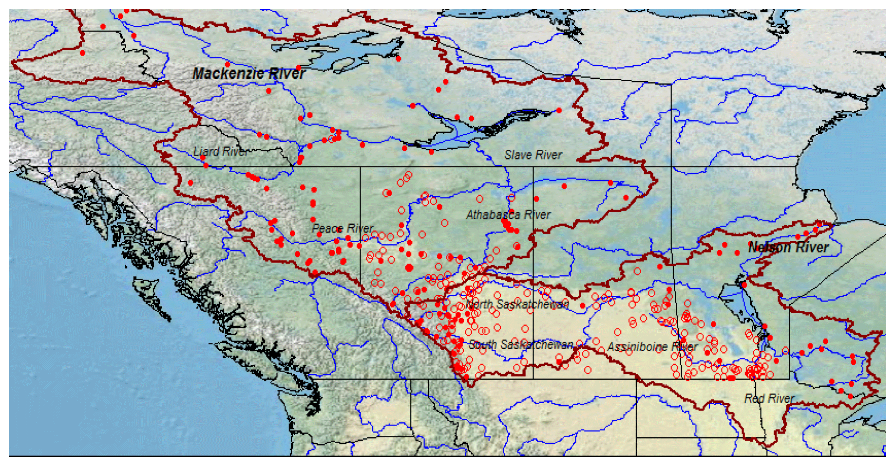
Figure 1 Study area showing the Mackenzie and Nelson River basins (dark-red outline) and the location of continuous stations (red dots) and seasonal stations (red circles). Basemap © OpenStreetMap contributors 2021. Distributed under a Creative Commons BY-SA License.

Table 1 Hydrometric stations included in the analysis. Only stations that are in these three basins were considered; to be included, they needed to be designated as having natural streamflow, being active, and having more than 30 years of record. The three other hydrometric stations were associated with a Changing Cold Regions Network Water, Ecosystem, Cryosphere, and Climate (WECC) Observatory with the number of years of record shown in parentheses.

Satellite imagery and derived spectral indices are valuable for assessing effects of environmental changes and the hydrological responses of the gauged basins; these methods allow determination of changes in vegetation, water bodies and snowcover for large areas (e.g. Hall et al., 1995; Hansen et al., 2013; Pekel et al., 2016; Su, 2000). Time series of spectral remote sensing indices were constructed using optical imagery from the TM sensor (USGS and NOAA, 1984) on the Landsat 5 satellite for each gauged basin. The satellite had a 16 d return period between 1985 and 2010 and acquired imagery for any location on the Earth's surface with a spatial resolution of 30 m. The sensor was selected for its spectral capabilities, which allowed evaluation of surface changes, and its long operation which best suits the length of the hydrological record in the gauged basins. It was chosen to avoid combining data from different satellites or sensors to maintain consistency in spectral response over the study period. Later satellites use different spectral bands.

2.2 Analysis

All analyses were performed with R (R Development Core Team, 2014) using packages kendall (McLeod, 2015), CSHShydRology (Anderson et al., 2018), and dtwclust (Sarda-Espinosa, 2017, 2018). A threshold of 0.05 was used in tests of significance, and accordingly, 5 % was also used as an indicator that the number of trends exceeds the number expected by chance alone.

As the intention was to include data from as many stations as possible, the entire period of record from each of the 395 gauged basins was used, and only the window where data were available from every station during the year from 21 April to 1 November was analysed. Table 2 provides the starting dates of the 5 d period corresponding to each 5 d period number from April through November. Because the station periods of record were used, rather than a common period of years, it was not appropriate to compare the magnitudes of trends among the stations. Instead, the analyses were restricted to determining the existence of significant trends in individual 5 d periods from 21 April to 1 November (periods 23 to 61, Table 2).

Table 2 Look-up table of 5 d periods during the annual common time window.

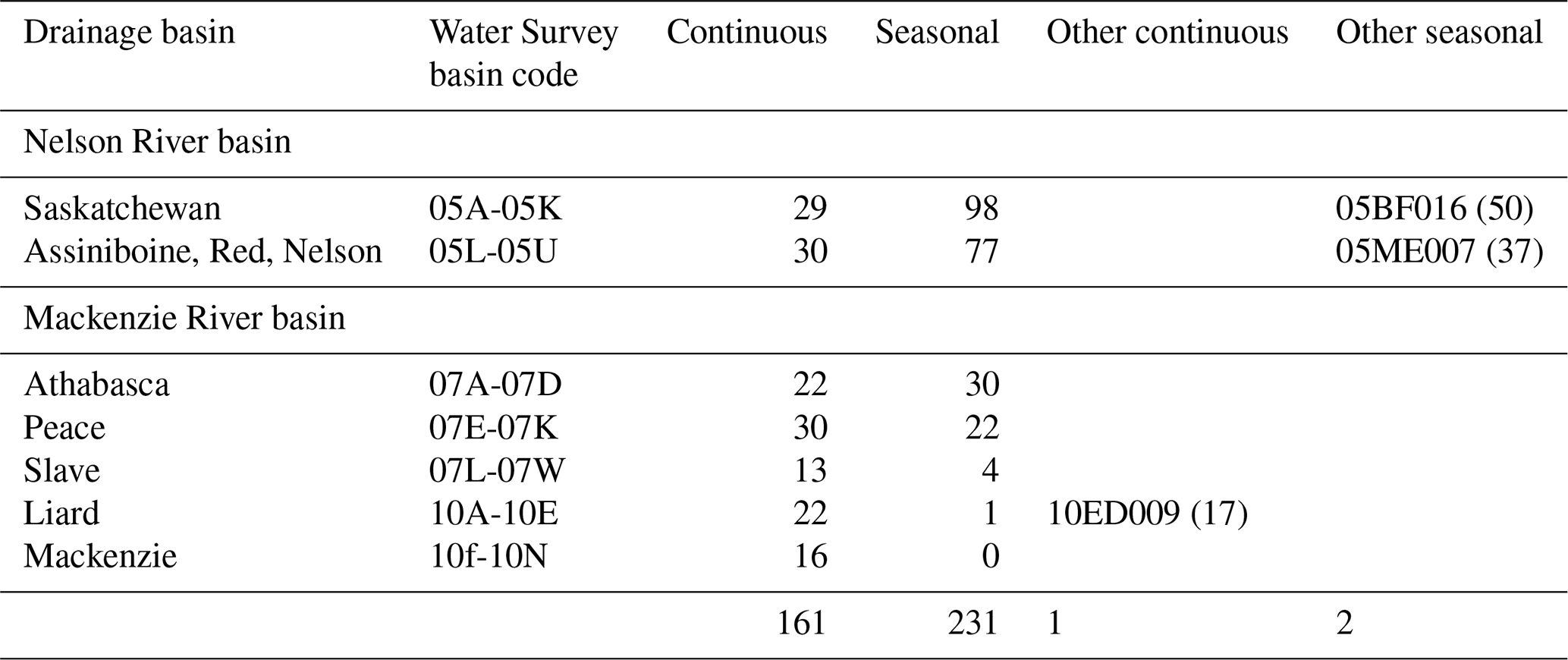
The main panel in Fig. 2 (bottom left) uses colour to show the magnitude of the flow for each day of each year for the Bow River at Banff, AB (stationID = 05BB001), an example of a long and complete continuous streamflow record from a national park in the Canadian Rockies. This streamflow record was described in detail in Whitfield and Pomeroy (2016, 2017). The upper panel of Fig. 2 shows the minimum, median, and maximum values for each 5 d period and blue (red) arrows indicate periods where there are significant increasing (decreasing) trends in streamflow over the period of record using Mann–Kendall tests. The directions of significant trends (i.e. positive or negative) were determined and were used subsequently for clustering of change types. The panel on the right shows the time series of annual minimum, median, and maximum discharges. If there was a significant trend (Mann–Kendall τ, p≤0.05), the series was coloured (red for decreasing, blue for increasing); black for no trend. The function for generating these plots was from CSHShydRology.

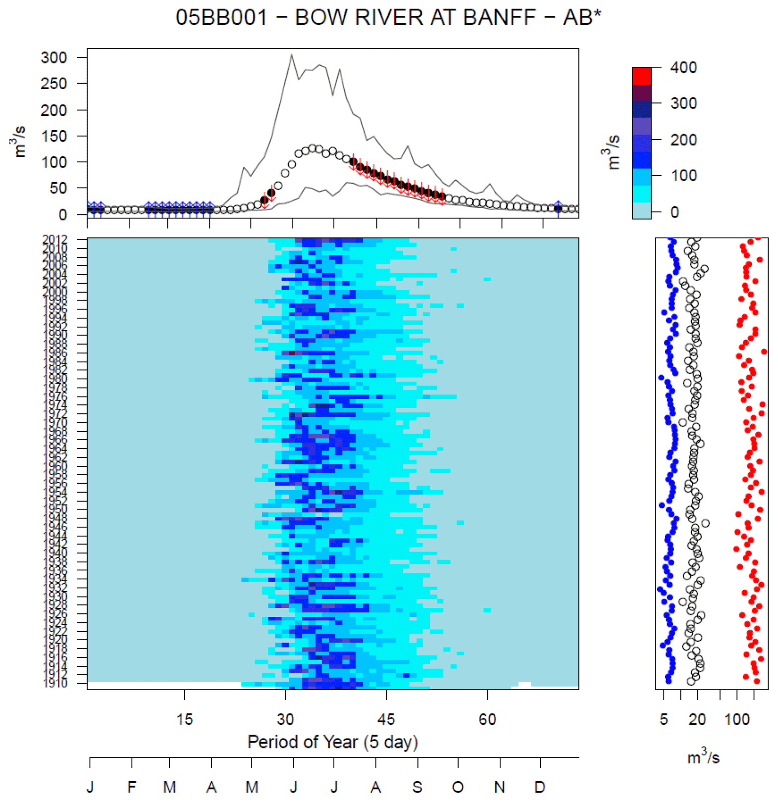
Figure 2 Plot of observed flows in the Reference Hydrologic Basin station 05BB001 Bow River at Banff, Alberta. The main panel shows the 5 d periods of the year against the years of record. White space indicates missing observations and the colours represent flow magnitudes scaled according to the bar in the upper right corner. The upper panel shows the maximum, median and minimum flow for each of the 5 d periods and red (blue) arrows indicate statistically significant decreases (increases) using Mann–Kendall τ at p≤0.05. The panel on the right-hand side shows the annual minima, median (open circle), and maxima; statistically significant decreasing (increasing) trends (Mann–Kendall τ at p≤0.05) are indicated by red (blue). Whenever the station is a member of the reference hydrologic basin network (RHBN), an ^* appears at the end of the station name.

The stations in this study were operated for differing periods of time and with differing operating schedules. Figure 3 provides an example for the Bow River at Lake Louise, AB (05BA001), a station upstream of the Bow River at Banff, showing that this station had continuous operation between 1910 and 1920, was discontinued from 1921 until 1963, operated continuously between 1964 and 1986, and then had seasonal operation between 1987 and 2013, hence records only exist during the warm season (Fig. 3). The seasonal trends shown in the upper panel are based on all years in which data were present in the 5 d periods. In the right-hand panel, trends over time in annual minima, medians, and maxima are based only upon the years with complete data, and this shows gaps in the time series. Trends of these types should be based only using years with complete records and are not addressed further since a large proportion of the stations have seasonal operation. Figures S2–S13 show up to four example hydrometric stations for each streamflow regime cluster, as described below. Many of these plots show stations where the operation has alternated between being seasonal and continuous, similar to Fig. 3. Figures S2–S13 also demonstrate the variation in the years of record between stations. The complexity of the data set results from historical budgetary and management decisions in the Canadian hydrometric program. Assessing hydrological regimes and trends in this data set requires approaches that are different from “standard” methods.

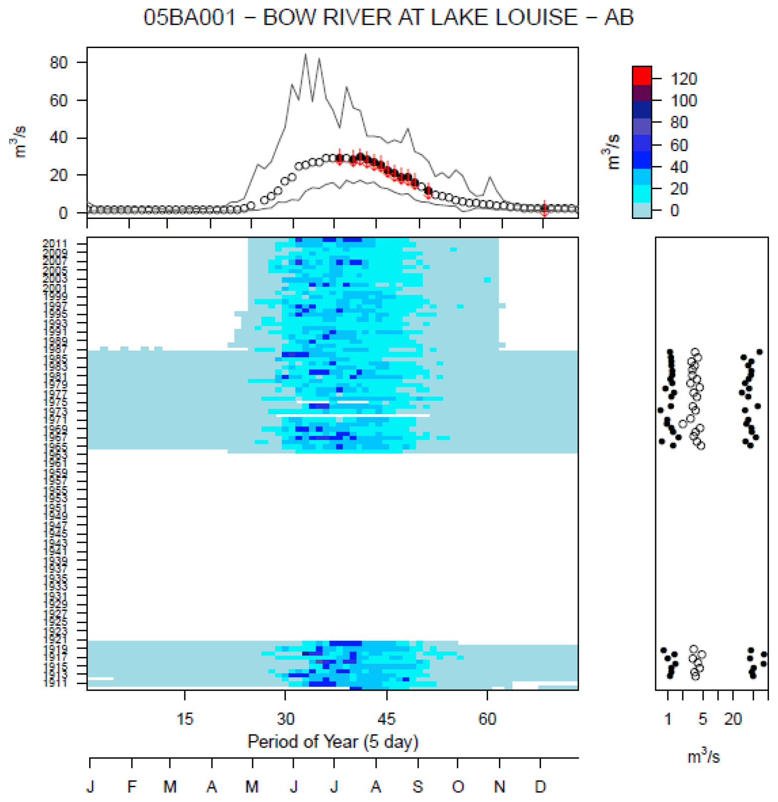
Figure 3 Plot of observed flows in the 05BA001 Bow River at Lake Louise, Alberta, a natural flow station. The main panel shows the 5 d periods of the year against the years of record. White space indicates missing observations and the colours are scaled according to the bar in the upper right corner. The upper panel shows the maximum, median and minimum flow for each of the 5 d periods and red (blue) arrows indicate statistically significant decreases (increases) using Mann–Kendall τ at p≤0.05. The panel on the right shows the annual minima, median (open circle), and maxima; statistically significant decreasing (increasing) trends (Mann–Kendall τ a p≤0.05) are indicated by red (blue).

2.2.1 Streamflow Regime Types

To avoid the effects of the areas of the gauged basins, the 5 d streamflow records were converted to z-scores by subtracting the mean value and dividing by the standard deviation of the series 5 d medians. The resulting series have means of zero and unit variance; plots of these were scaled in magnitude by the standard deviations (e.g. Fig. 4). Early snowmelt at low latitudes and elevations resulted in some stations having flow events prior to the annual common time window (Fig. 4). Only the data in the periods between the two vertical dashed lines in Fig. 4 (5 d periods 23 to 61) were used in the clustering (and subsequent trend analysis) reported here. The use of 5 d means is based on previous work (Leith and Whitfield, 1998, Déry et al., 2009b) to place the analysis at a common time step across all sites and to balance the variation in hydrologic signatures of basins of different sizes while avoiding information loss that occurs with smoothing at seasonal and monthly time steps (Whitfield, 1998).

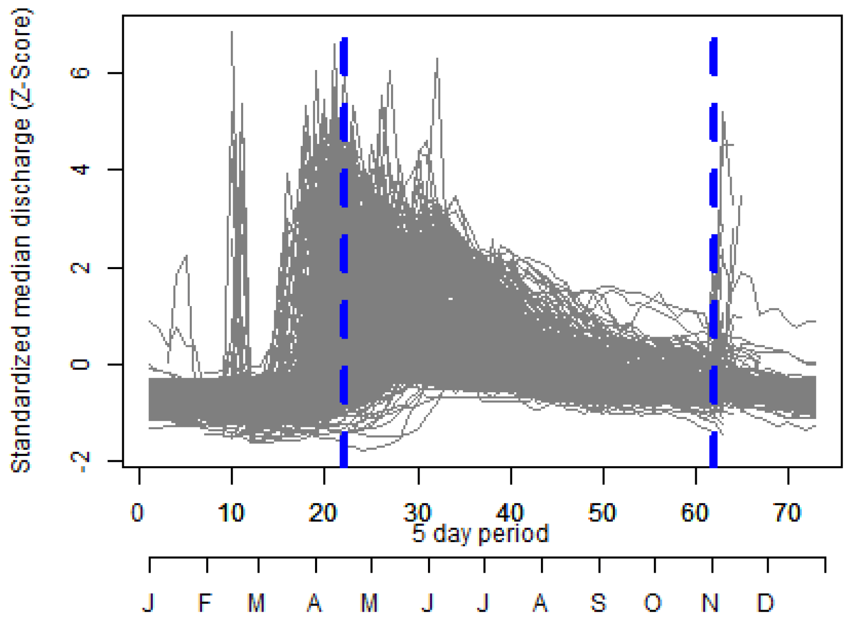
Figure 4 Standardized median streamflow for 5 d periods from the 395 hydrometric stations. The flow from each station was standardized by removing the mean and dividing by the standard deviation. Only the period between 21 April and 1 November (indicated by the region between the blue dashed lines) is considered, as seasonally operated stations have no observations during winter months.

Statistical methods, such as k-means (Likas et al., 2003; Steinley, 2006) or self-organized maps (Kohonen and Somervuo, 1998; Hewitson and Crane, 2002; Kalteh et al., 2008; Céréghino and Park, 2009; van Hulle, 2012), are unable to group hydrographs when they are not aligned in time (Halverson and Fleming, 2015). Across the study domain this is a difficulty, as the timing of snow accumulation and melt are strongly affected by both latitude (48 to 69^∘ N) and elevation (near sea level to > 2100 m), reflecting the seasonal variation in the 0^∘ isotherm (Mekis et al., 2020).

The clustering of annual median streamflow time series was done using dynamic time warping, DTW (Berndt and Clifford, 1994; Wang and Gasser, 1997; Keogh and Ratanamahatana, 2005), which measures similarity between time series that may vary in magnitude and timing by aligning the two standardized (zero mean, unit variance) curves in time, essentially matching the shape of inflections to create clusters (Sarda-Espinosa, 2017; Whitfield et al., 2020).

As an example of the DTW alignment, the z-scores of the median streamflows from two stations, the semi-arid foothills and grassland-sourced Snake Creek near Vulcan, AB (05AC030), and Arctic tundra-sourced Anderson River below Carnath River, NT (10NC001), are aligned in Fig. 5. The two curves differ in the timing and magnitude of their peaks (Fig. 5a); the DTW distance calculated is a dissimilarity measure constructed from a warping path based upon the matching of inflections between the two curves (Fig. 5b) essentially matching the shape of inflections and shifting the curves to a common time frame (Fig. 5c). R package dtwclust (Sarda-Espinosa, 2017) implements dynamic time warping to cluster multiple curves based upon their having similar shapes and inflections and was used for clustering the 395 cases in this study. The timing of inflections does not affect the clustering, so the effects of latitude and elevation that often result in misclassification of hydrographs because of timing differences are avoided. This is important given the size of the spatial domain considered here. A 12-cluster solution was chosen; this number of clusters balances regional separation of similar hydrograph types while avoiding producing many types with single stations which represent unique hydrological situations. “Streamflow Regime Type” in the text which follows refers to these 12 clusters.

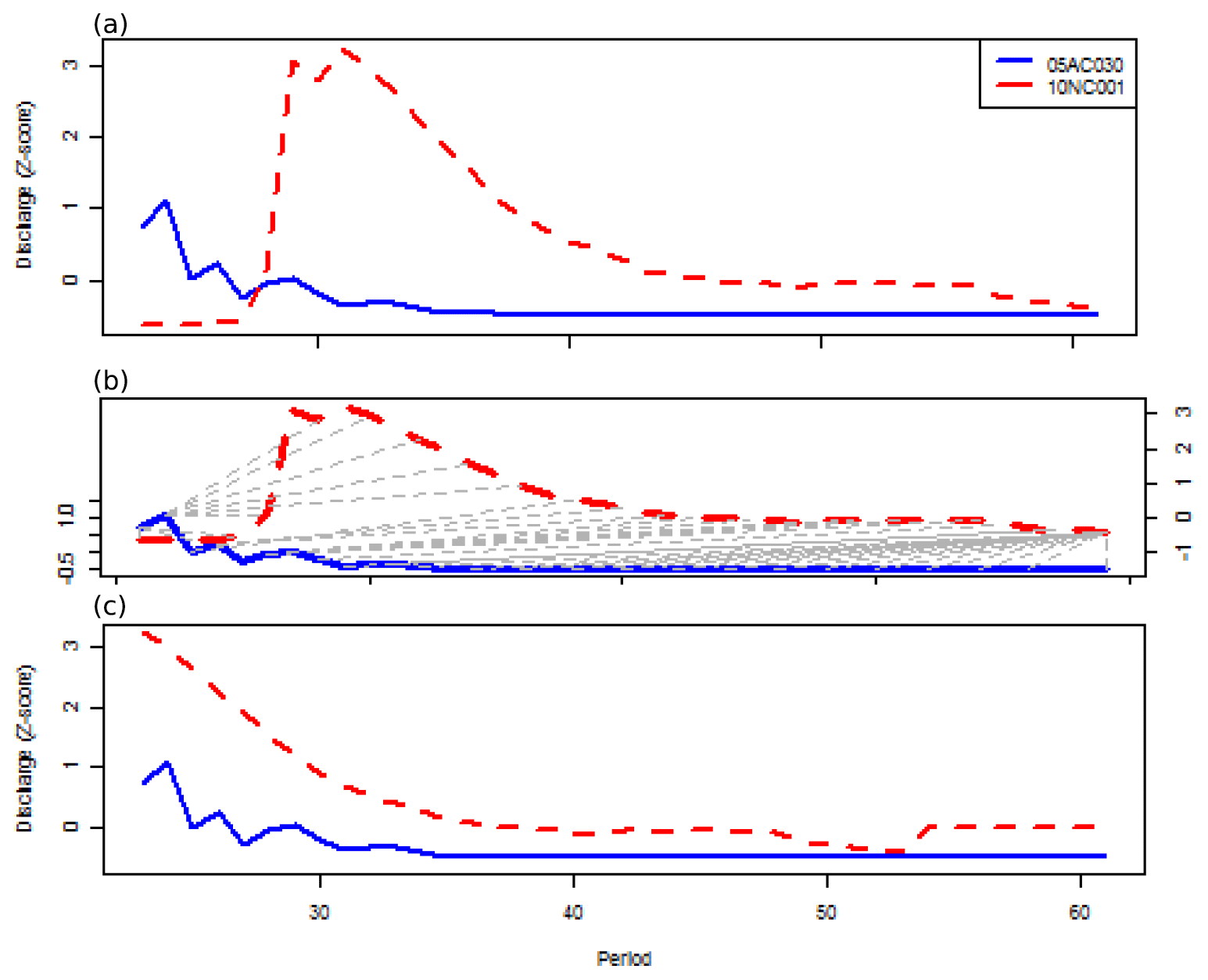
Figure 5 Example of alignment of two time series using dynamic time warping (DTW) from stations 05AC030 Snake Creek near Vulcan, AB, and 10NC001 Anderson River below Carnwath River, NT.

The centroids of each regime type provide insight into differences in regional hydrology. The shape of the centroid and the recession slope(s) of the curves provide information that can be used to further compare differences between clusters.

2.3 Trend Patterns

Trends in each of the 5 d periods for the annual common time window were determined for the period of record of each time series, using Mann–Kendall tests as described above, following the approach of Déry et al. (2009b) for examining trend magnitude for a fixed endpoint in time. Interpreting the results for any fixed time period may not be representative of a longer timescale (Hannaford et al., 2013). As these were comparing periods separated by 360 d, i.e. a resampled time series, autocorrelation was not expected, and therefore pre-whitening was not applied. Tests with 100+ years of record show that nearly 90 % of cases did not show autocorrelation, and the balance was close to the level of significance (0.19). The individual station trend test results are indicated in the upper panels of Figs. 2, 3, and S2–S13, where significant increases and decreases are indicated by blue and red arrows respectively. The significant increasing, no trend, and decreasing trends were assigned scores of 1, 0, and −1 respectively. The individual annual trend scores for the annual common time window for the 395 stations were clustered using the method of k-means, which partitions observations into clusters having similar means and which is well suited to clustering of features such as patterns of significant differences (Likas et al., 2003; Steinley, 2006; Agarwal et al., 2016). The number of clusters chosen (six) was based upon the elbow method (Ketchen and Shook, 1996; Kodinariya and Makwana, 2013); using more than six clusters did not improve the modelling (not shown). These six clusters are hence referred to as “Trend Patterns”.

As the method used here is unconventional, we assessed how the patterns of trends would differ when using varying periods of record. Trends in each of 39 5 d periods were first determined for the entire period of record and were then compared to those of 21 periods, with lengths decreasing by 5 years between 1905 and 2005 (e.g. 1905–2015, 1910–2015, 1913–2015). Eleven stations with more than 3 years of data in the final interval (2005–2015) were excluded so that missing values were not introduced. The ∼ 15 000 comparisons (384 sites for 39 5 d periods) were used to determine the number of cases where the trends did not change. These comparisons were also tested using a classification approach and the adjusted Rand index (Morey and Agresti, 1985) and produced similar results (not provided here).

2.4 Trends in vegetation, water, and snow satellite indices

Given the large study region and the long study period, analyses of time series of Landsat 5 TM data are very resource intensive, both in terms of storage and computational power, and are beyond the scope of desktop computing. Google Earth Engine (GEE) allows for cloud-based planetary-scale analysis, while it serves as a database for petabytes of open-access satellite imagery such as the Landsat archive (Gorelick et al., 2017) and is particularly capable for this study.

Using GEE, Landsat 5 TM image composites (n= 579) were produced to cover the spatial extent of all the gauged basins for the period between 1985 and 2010 by mosaicking the available image scenes for each consecutive 16 d period. Theoretically this would allow for spatially complete mosaics given the 16 d revisit time of the satellite. To determine accurate spectral indices at the basin scale, pixels containing clouds or cloud shadows in each image scene were masked prior to mosaicking using the GEE-integrated Fmask algorithm (Zhu et al., 2015), which introduced intermittent data gaps to the set of mosaics. Additional data gaps were caused by occasional unavailability of satellite image scenes in the Landsat 5 TM catalogue, typically due to image quality or georeferencing issues (USGS and NOAA, 1984). To reduce the computation cost and data volume, the final mosaics were generated at an aggregated spatial resolution of 300 m. The total number of satellite image scenes used was 83 381.

For each basin, three time series of spectral index averages were derived from the 16 d mosaics of Landsat 5 TM data. Each normalized difference index (I) compares two wavelength ranges (W1 and W2) observed by the satellite detectors, using the form I = (W1 − W2)$/$(W1 + W2), each index ranging between −1 and 1. The three common indices used were the Normalized Difference Vegetation Index (NDVI), Normalized Difference Water Index (NDWI), and Normalized Difference Snow Index (NDSI) (Lillesand et al., 2014) and were calculated by

$$\begin{array}{}\text{(1)}& {\displaystyle }\mathrm{NDVI}=\left(R_{\mathrm{NIR}}-R_{\mathrm{Red}}\right)/\left(R_{\mathrm{NIR}}+R_{\mathrm{Red}}\right),\text{(2)}& {\displaystyle }\mathrm{NDWI}=\left(R_{\mathrm{NIR}}-R_{\mathrm{SWIR}}\right)/\left(R_{\mathrm{NIR}}+R_{\mathrm{SWIR}}\right),\mathrm{and}\text{(3)}& {\displaystyle }\mathrm{NDSI}=\left(R_{\mathrm{Green}}-R_{\mathrm{SWIR}}\right)/\left(R_{\mathrm{Green}}+R_{\mathrm{SWIR}}\right),\end{array}$$

where R is the dimensionless top-of-atmosphere reflectance, Green is TM band 2 (green light 0.52–0.60 µm), Red is TM band 3 (red light 0.63–0.69 µm), NIR is TM band 4 (near infrared 0.76–0.9 µm), and SWIR is TM band 5 (shortwave infrared 1.55–1.75 µm). Because of the presence of the masked cloud pixels and data gaps, the basin means were often only calculated from a fraction of the complete pixel set of the basin; this fraction was determined for every observed time step.

For each 16 d period, the mean NDVI, NDWI, NDSI, and fractional coverage were determined for each of 375 gauged basins for which a shapefile of basin boundaries was available (20 basin boundaries were not available from Water Survey of Canada). A sample data set is shown in Fig. S14. Time series of annual maximum, mean, and minimum were determined for each of the normalized different indices and their fractional coverages from these data sets. Since there were only ∼22 images (at most) available for each year in each basin, the entire year was used rather than the annual common time window so that the annual minimum, maximum, and mean would be comparable across the study domain.

Forkel et al. (2013) demonstrated the annual variability of NDVI time series and the effects of using different analysis methodologies. Verbesselt et al. (2010, 2012) and de Jong et al. (2012) used breaks for additive season and trends (bfast) to detect change, particularly phenological change, in satellite imagery; bfast iteratively estimates the time and number of abrupt changes within time series derived from satellite images. While this methodology has considerable appeal and has been used widely and successfully to assess change in target areas, it was impractical to apply bfast here as it is difficult to summarize multiple changes in seasonality, trends, and breakpoints for three indices across 375 basins. A simpler approach, testing for simple trends in the mean, maximum, and minimum indices using Mann–Kendall (McLeod, 2015), avoids the rich complexity possible with bfast but still illustrates that NDVI, NDWI, and NDSI changes were accompanying streamflow regime changes. The minimum NDSI values excluded zero values.

3 Results

3.1 Streamflow Regime Types

The Streamflow Regime Types from the 12-cluster solution are shown in Fig. 6. Each of the 12 plots contains a line for each gauged basin in that type, and the heavy dashed line, where visible, is the centroid of all members; the colour of the lines is based upon stationID. The x axis is time, shown in increments of 5 d periods; these periods are renumbered starting with 1 for period 23. The y axis is the z-score (standard deviation units); the series for each site was converted to a z-score subtracting the mean and dividing by the standard deviation. The differences in the shapes of the hydrographs between regime types are evident and demonstrate how the shapes of the members and locations within a Streamflow Regime Type were similar. The outlying individual cases (e.g. Streamflow Regime Types 6, 7, and 8) are also evident.

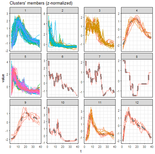
Figure 6 Streamflow Regime Types produced by clustering of the 395 standardized median 5 d streamflows using dynamic time warping. The individual lines are coloured based on stationID; the consistency of colour reflects similar spatial locations. The heavy dashed line is the centroid of the cluster. Note that the number on the x axis is for the aligned series (1–39) as opposed to 23–61. The y-axis value is the z-score and differs in scale between the panels.

Example plots for each of these 12 Streamflow Regime Types are shown in Figs. S2 to S13 to illustrate the similarity and differences between the hydrographs within the streamflow regime types. Streamflow Regime Type 1 basins were generally Rocky Mountain basins that have strong snowmelt and spring rainfall maxima signals (Fig. S2). Streamflow Regime Type 2 basins were reflective of Prairie streams with spring snowmelt and long periods with low or zero flow due to summer water deficits, variable contributing areas, and frozen conditions in winter (Fig. S3). Streamflow Regime Type 3 basins were in the Athabasca River basin dominated by humid upland boreal forest and lowland muskeg (Fig. S4). Streamflow Regime Type 4 (Fig. S5) has both strong snowmelt and late-summer streamflow. Streamflow Regime Type 5 basins were predominantly in the sub-humid Boreal Plains mixed forest (Fig. S6). Basins of Streamflow Regime Types 6–8 and 10 were unique (or nearly so) but were similar to adjacent types (Figs. S7, S8, S9, and S11). An interesting feature of these four types is that peak flows occur at different times in different years. Streamflow Regime Type 9 basins peak later in the summer and were generally smoother than for other basins (Fig. S10). Streamflow Regime Type 11 basins have an early snowmelt peak and high flows extending through into the fall (Fig. S12). Streamflow Regime Type 12 basins have an early snowmelt peak and persistent high flows during summer and extend into the fall (Fig. S13).

The spatial extents of the 12 Streamflow Regime Types were mapped over ecozones in Fig. 7; there is a clear spatial organization rather than a random pattern. This association is also evident in Table 3. Two large-scale features are evident: similar types tend to be from the same spatial areas, and some similar types follow along major rivers. Streamflow Regime Types 3 and 11 follow along rivers and Types 2 and 5 overlap. Streamflow Regime Types 1 (104 members) and 5 (148) occur in the greatest numbers of ecozones (8 and 6 respectively; Table 3).

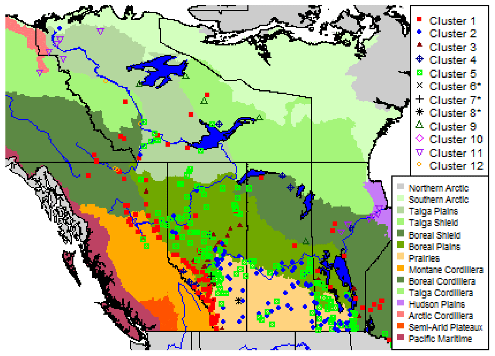
Figure 7 Locations of the 12 Streamflow Regime Types from the changing cold-region domain overlain on the ecosystems of Western Canada. Clusters marked with an ^* have only a single member.

Table 3 Streamflow Regime Type classification in relation to the ecozone in which the station is located.

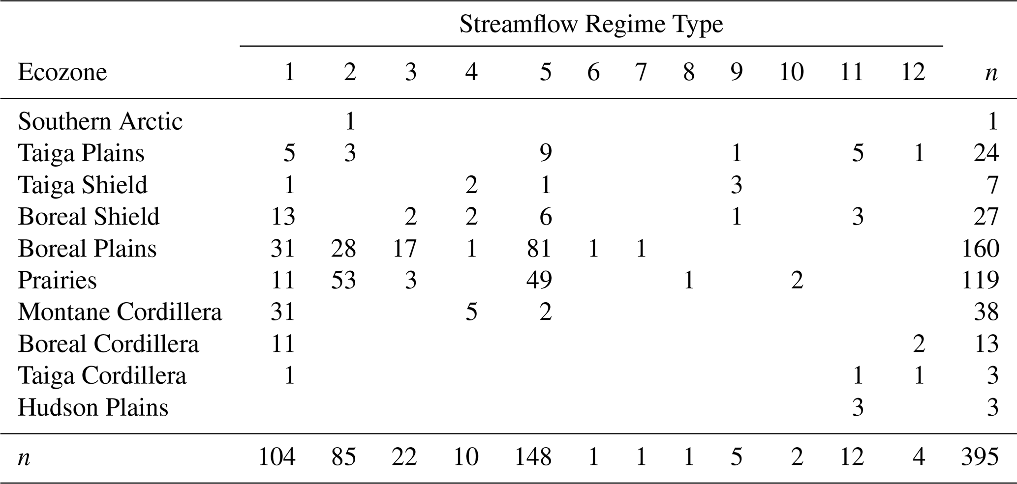
Streamflow Regime Type 1 basins occur in the Cordillera (Montane n= 31 basins, Boreal n= 11, and Taiga n= 1) and also the Boreal Plains (n= 31), Taiga Plains (n= 5), Boreal Shield (n= 13) and Prairies (n= 11); the Type 1 hydrograph shows a sharp, brief melt period followed by a long, slow recession (Fig. 6). Streamflow Regime Type 5 basins were also common in the Prairie ecozone (n= 49), in the Boreal Plains (n= 81) as well as along the Mackenzie River to below Great Slave Lake; the hydrograph for this type shows an earlier and briefer peak than Type 1, with a rapid recession (Fig. 6). Streamflow Regime Type 4 basins (n= 10) were predominantly found in the Montane Cordillera in the west (n= 5) and in the Boreal Shield and Boreal Plains in the east (n= 2 each); the hydrograph shows prolonged high flows during the melt period and a short recession with relatively large flows (Fig. 6). Streamflow Regime Type 3 basins (n= 22) appear in the Boreal Plains (n= 17), Boreal Shield (n= 2) and Prairies (n= 3) and demonstrate the persistence of a mountain runoff signal along the Athabasca River, as this hydrograph contains the late-melt signal from glaciers and high-elevation snowpacks (Fig. 6). Streamflow Regime Type 2 basins (n= 85) were associated with the Prairie ecozone (n= 57) and Boreal Plains (n= 28), but this pattern also occurs in the Southern Arctic (n= 1) and Taiga Plain (n= 3); this pattern has the earliest snowmelt and most rapid recession, and the records often begin with snowmelt already in progress (Fig. 6). Streamflow Regime Type 11 basins (n= 12) were located near the mouth of the Mackenzie in the Taiga Plains and in the Hudson Plains along the Nelson River in Manitoba. Streamflow Regime Type 12 basins (n= 4) were in the Boreal Cordillera. Streamflow Regime Type 6–8 basins (1 each) and 9 (n= 2) were located at the edges of ecozones. While these descriptions are explicit, there was overlapping of types in space (particularly Streamflow Regime Types 2 and 5) and cases where individual basins of a type occur quite separately from each other (Types 9 and 12), as is evident in Fig. 7.

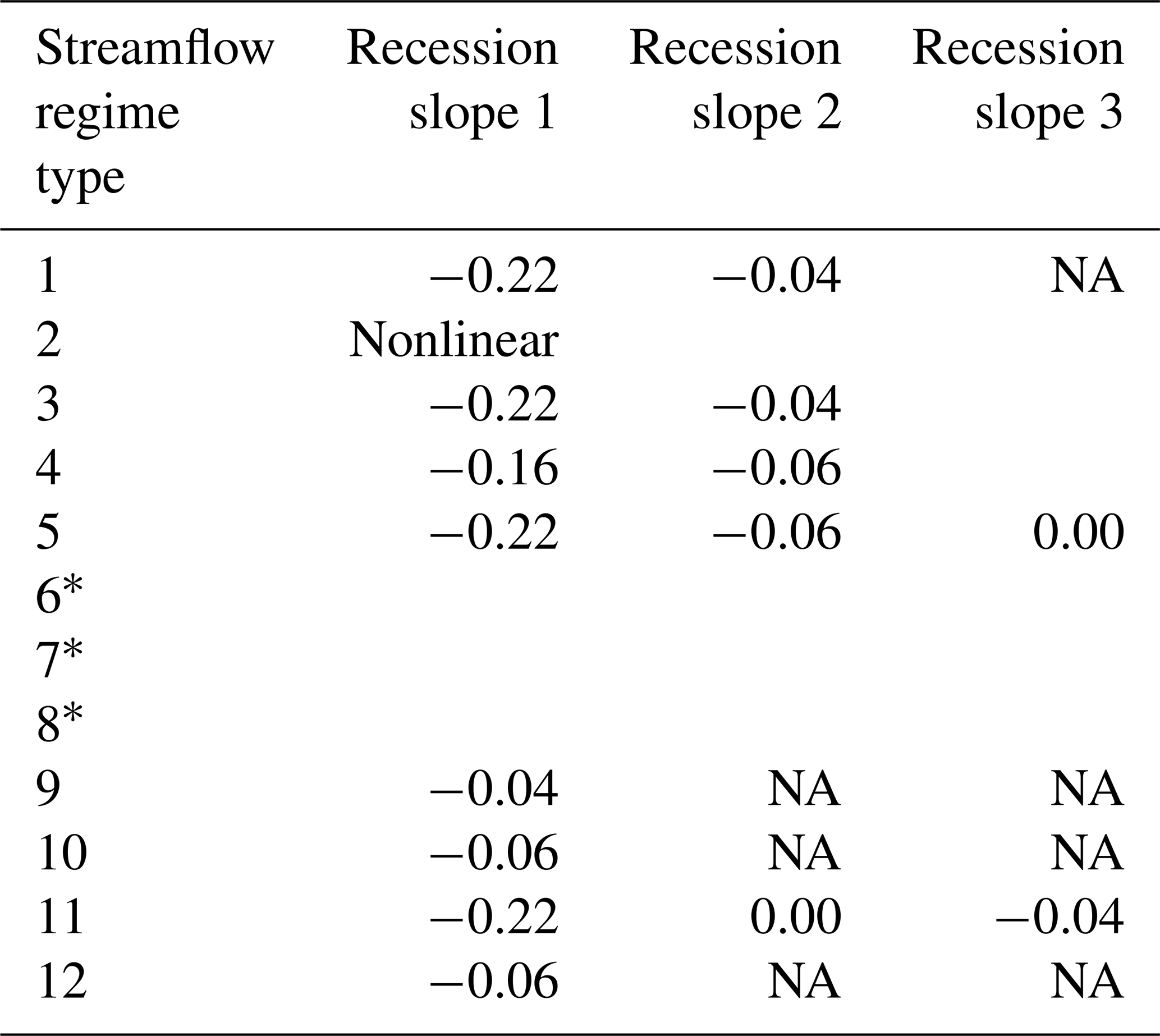
The standardized streamflows plotted in Fig. 6 make it difficult to compare the Streamflow Regime Types; plotting the z-score centroids of each (Fig. 8) makes the comparisons simpler. The non-Prairie Streamflow Regime Types have approximately linear recessions with two slopes (Types 1, 3, 4, and 12) or more (Type 11). The slopes of the recessions are listed in Table 4. Typically, the first recession phase was steeper than the second phase – where there was one. In Streamflow Regime Type 11 the third phase was steeper than the second but not as steep as the first. After a rapid recession, Streamflow Regime Type 2 becomes nearly horizontal, probably due to Prairie streams typically having no base flows due to lack of groundwater contributions. In Streamflow Regime Type 5 the recession has two linear phases and also terminates in a horizontal section, which was again likely to be caused by the absence of base flows in many Prairie basins. These recessions appear to have only five values, two that were steep (−0.22 and −0.16) and two that were much flatter (−0.06 and −0.04) in addition to the zero slope (no slope) of Type 5.

Figure 8 Centroids of the 12 Streamflow Regime Type clusters.

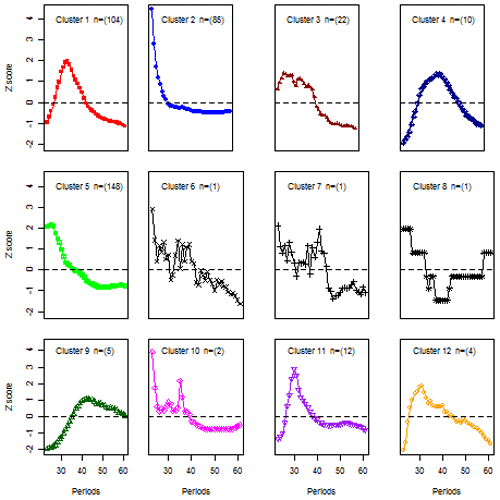
Table 4 Summary of recession slopes amongst the 12 Streamflow Regime Types. Units are z-score/length estimated from Fig. 8. Types with ^* have only one member and are excluded here. NA means not available.

A caution is warranted here. The shapes of hydrographs are controlled by the climate, hydrological processes and landscape predominantly in the area of the basin where most of the runoff is generated, and while association with an ecozone was useful, the ecozone is a generalization and does not always capture hydrological functions in the source areas. In many rivers, the source of runoff lies in the high mountains, and these patterns are transmitted along the downstream river course such as in the Mackenzie, Liard, Athabasca, and Nelson rivers. Such stations are not independent. Differences between Streamflow Regime Type 1 and 4 basins likely reflect low late-summer flows from parts of the Rocky Mountains. In areas where there was overlap between different Streamflow Regime Types, both similarities and differences exist between the basins.

3.2  Trend Patterns

Trend Patterns are based upon the statistical trends in 5 d flows discussed above. Figure 9 illustrates the trend results for one station, 05DA007 Mistaya River near Saskatchewan Crossing, which drains a heavily glaciated mountain basin that is undergoing deglaciation. In the case of Fig. 9 there were three periods (39, 40, and 46) in July and August with significant decreases; the other periods have no trends.

Figure 9 Example of the trend portion of the summary hydrograph: the two dashed lines indicate the start and end of the common window from period 23 to period 61.

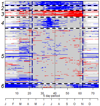
Figure 10 Trend patterns in the 395 stations, significant increases (blue) and significant decreases (red), no trend (gray) and missing (white). The stations are ordered by Trend Pattern (cluster) number and stationID. Data outside the dashed lines were not used in the clustering but are shown where available (periods 1–22 and 62–73).

Figure 10 plots all significant trends for the 395 basins, with significant increases and decreases shown in blue and red, no trend in gray, and no available data in white. These data were ordered by the six Trend Patterns determined using only the data for the 5 d periods from 23 to 61; Fig. S15 shows the data order by stationID. Periods 1–22 and 62–73 were not included in the clustering but were plotted as they are also of interest.

Trend Patterns in Fig. 10 are presented in the order that clusters were formed, showing the distinctly different Trend Patterns 1, 2, 3, 4, and 6, while Trend Pattern 5, the largest group with more than 250 basins (64 % of the total), does not have a consistent organized change despite there being individual periods with increasing or decreasing trends. Trend Pattern 1 shows positive streamflow trends in most of the annual common time window, suggesting a general increase in wetness throughout the spring, summer, and fall. Trend Pattern 2 has positive trends, suggesting increased wetness after period 30 in early summer. Trend Pattern 3 has predominantly significant negative trends, with many more in periods 40–61 than in periods 23–39, suggesting decreases in late-summer and fall streamflow. Trend Pattern 4 has significant increases centred about period 35, suggesting a shift increased snowmelt and rainfall-runoff peaks in June. Trend Pattern 6 shows significant increases in the first periods and last periods of the window but not during the summer; this group of stations all have winter data and show increasing streamflow throughout the late fall, winter, and early spring periods.

The trends presented in Fig. 10 are based on 39 5 d periods using the available data seta with records of at least 30 years. The stability of the trend results with decreasing-length observation periods is demonstrated in Fig. 11, where the trends are compared for increasingly shorter time periods with the results for the entire period. The fraction of the approximately 15 000 reduced-period results that are the same as the complete-period results is greater than 0.75, even when the record length is reduced to 10 years. The mean fraction of sites showing significant trends detected in each time period is about 0.20 and is at a maximum at 35 years and decreases at shorter time intervals (Fig. 11). For a period of 10 years, 5 % of the cases show significant trends, as would be expected by chance alone (based on a p value of ≤ 0.05). The impact of reduced length affects the Trend Patterns differently. Trend Patterns 1 to 3 show greater changes in the fraction of significant trends than Trend Patterns 4 to 6 (Fig. 11).

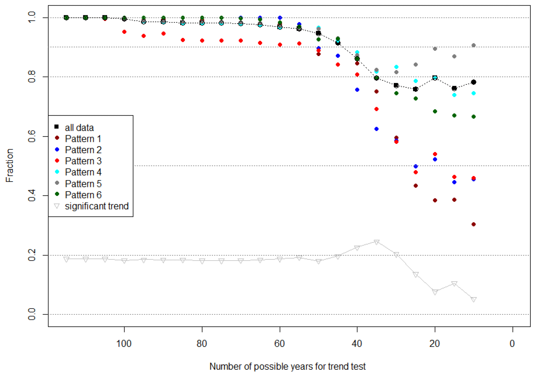
Figure 11 The fraction of stations with the same Trend Pattern as in the original full-length record for period lengths decreasing from 115 to 10 years in 5-year steps. The fraction for all data is plotted as filled black squares and for each of the six Trend Patterns as filled circles (colours are as in other figures). The fraction of stations with a significant trend for each step is plotted as gray triangles. This analysis was done using 384 sites of the original 395; the 11 sites omitted had less than 3 years' worth of observed values in the final time period (2005–2015).

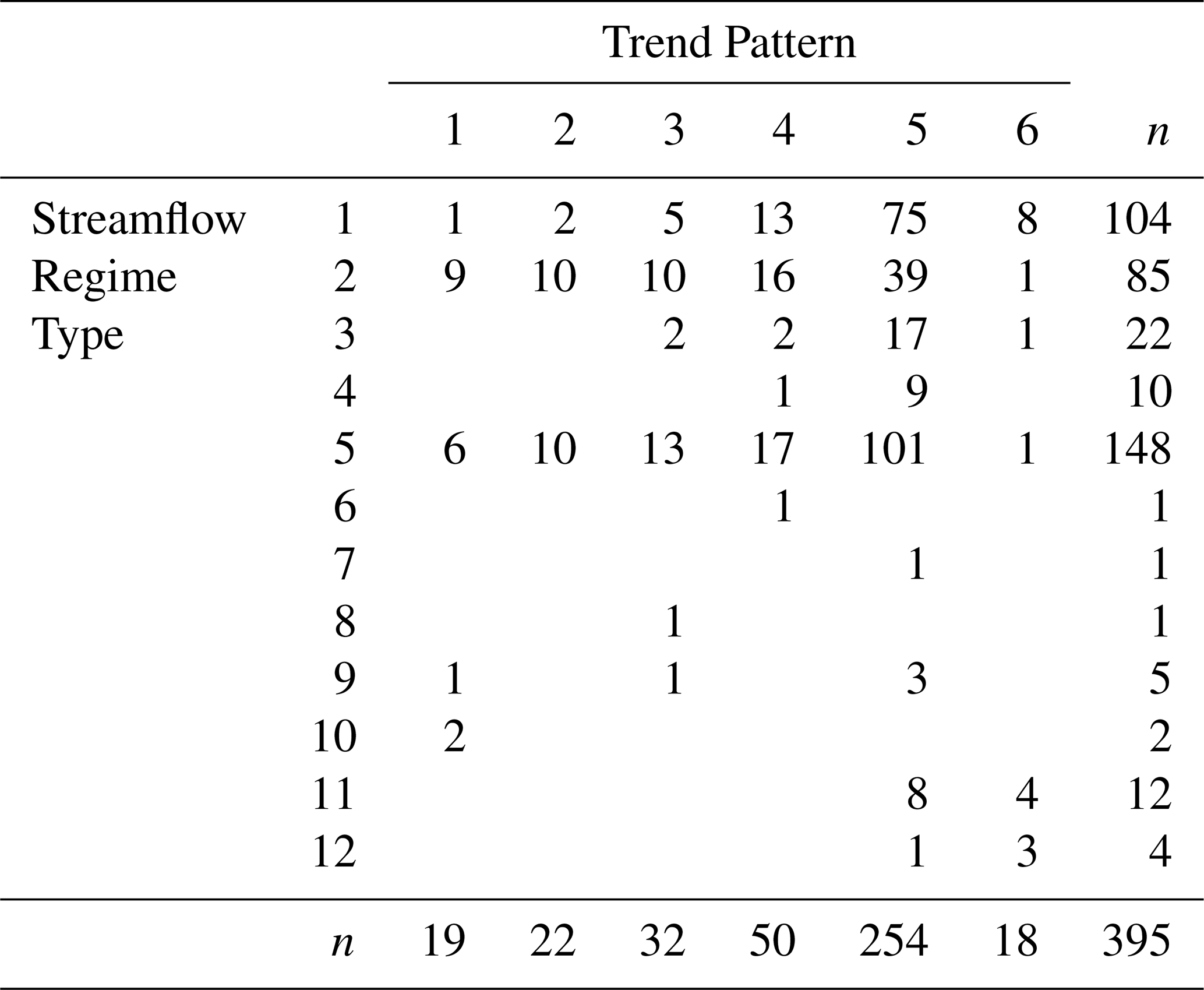
Associating a Trend Pattern with a Streamflow Regime Type is complicated as there were different numbers of basins in the Streamflow Regime Types and Trend Patterns (Table 5). Trend Pattern 5, which lacks any pattern, was very prominent in most of the Streamflow Regime Types having many members. Again, the caution regarding rivers sourced in the mountains and propagating the upstream signal downstream in nested basins also applies to their Trend Pattern as well.

Table 5 Trend Patterns for 395 stations against their Streamflow Regime Type classification.

The six Trend Patterns of the 395 hydrometric stations are mapped to ecozones in Fig. 12. Supplement Figs. S16–S21 provide more detail on the individual Trend Patterns and the station locations. Trend Pattern 1 (n= 19, S16) basins were located at the eastern and western margins of the Prairies with two north of 60^∘, all showing increasing streamflows throughout the entire year. Trend Pattern 2 (n= 22, S17) basins, with early summer increases, were located across the Prairies and in the eastern portion of the Boreal Plain. Trend Pattern 3 (n= 32, S18) basins, showing decreased streamflow, were located predominantly in the western portions of the Boreal Plain and on the eastern edge of the Montane Cordillera. Trend Pattern 4 (n= 50, S19) basins, with larger early summer peaks, were located across the Prairies largely along the northern edge adjacent to the Boreal Plains and in a few northern locations in the Boreal Plain. Trend Pattern 5 (n= 254, S20) does not show an organized change pattern in the annual common time window and was distributed across all the ecozones. Trend Pattern 6 (n= 18, S21) basins, with higher cold and cool season flows, were located entirely in northern areas in the Taiga Plains, Taiga Shield, and Taiga and Boreal Cordillera. Overall, 28 % of the basins show one of the four increasing Trend Patterns, and 8 % have the single decreasing pattern.

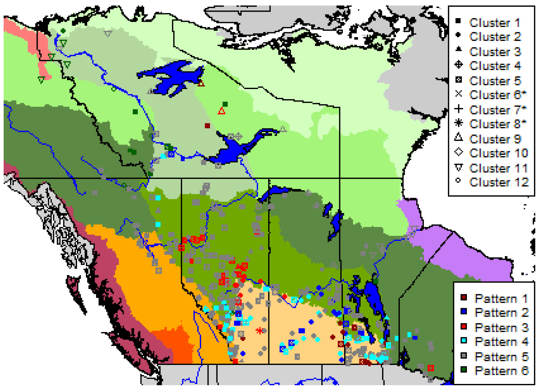
Figure 12 Trend Patterns (colour) and Streamflow Regime Types (cluster no. with symbols) of the 395 stations in the study domain. The ecozone legend is as in Fig. 7.

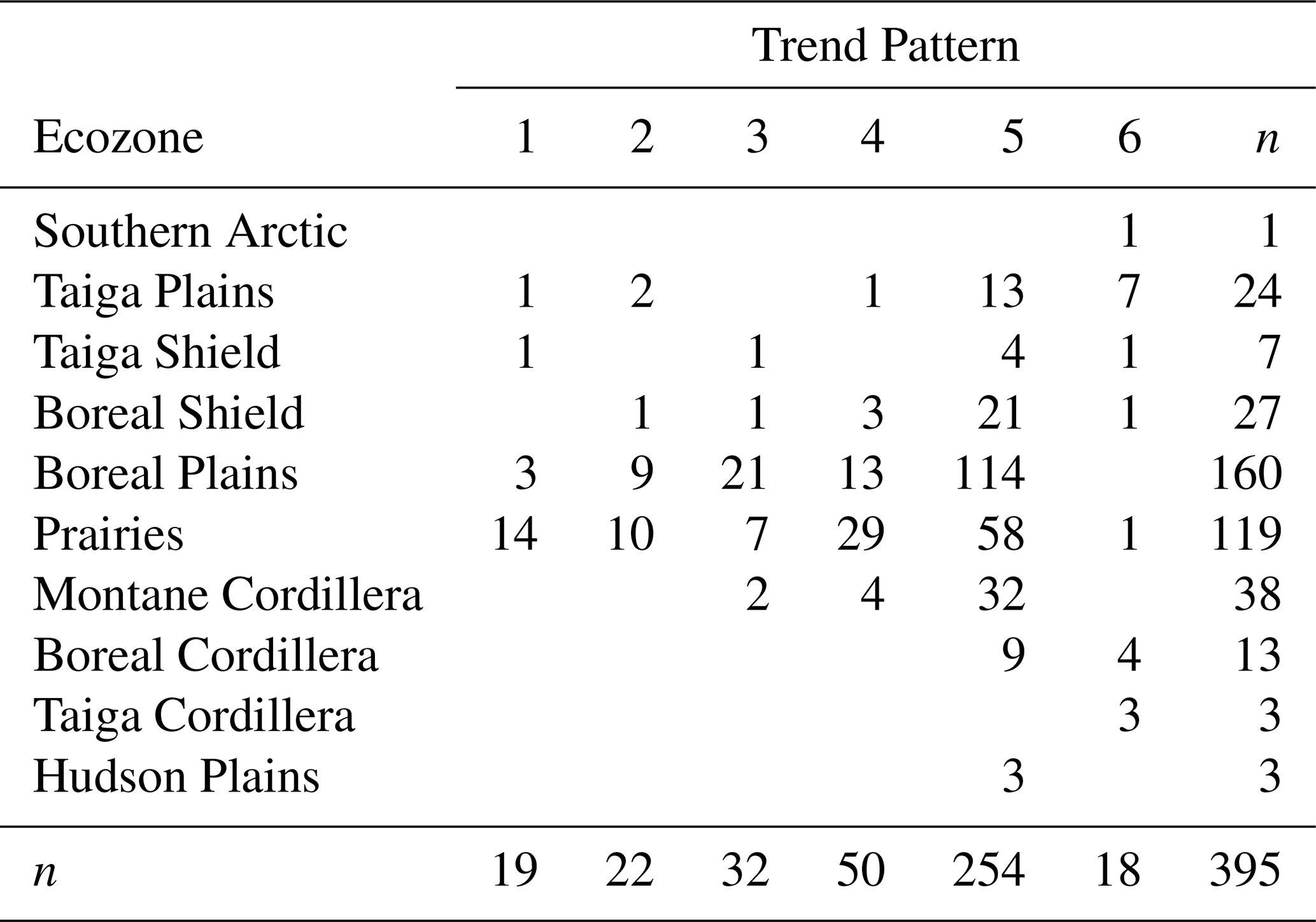
At the ecosystem scale, 51 % of basins in the Prairies exhibit a definite Trend Pattern, with 45 % showing one of the increasing patterns (Trend Patterns 1, 2, 4, and 6) and 6 % the decreasing Trend Pattern 3 (Table 6). In the Taiga, increasing Trend Patterns predominate, with 46 % of stations in the Taiga Plains showing increasing patterns and none with the decreasing Trend Pattern, 29 % of the Taiga Shield having an increasing Trend Pattern and 14 % a decreasing Trend Pattern, and all three of the Taiga Cordillera basins having increasing Trend Patterns (Table 6). The Boreal Shield and Plains have increasing Trend Patterns in 16 % of stations and decreasing Trend Patterns in 13 %. The Boreal and Montane Cordillera have increasing Trend Patterns in 11 % of basins, and only the Montane Cordillera had the decreasing Trend Pattern (5 %) (Table 6). Trend Pattern 6 only occurs in the northern portion of the study area, which is dominated by thawing permafrost. None of the stations on the Hudson Plains showed any Trend Pattern. These results indicate that the streamflow regime change has a spatial basis, influenced by the location and ecozone, rather than by the Streamflow Regime Type.

Table 6 Trend Patterns in relation to the ecozone in which the station is located.

3.3 Trends in vegetation, water, and snow satellite indices

The spatial patterns of trends in the mean values of the three normalized difference indices are presented in Fig. 13. The spatial patterns of the trends in the maximum, mean, and minimum of NDVI, NDWI, and NDSI are provided in Figs. S22–S24 and are also summarized in comparison with Streamflow Regime Type (Table 7), Trend Pattern (Table 8), and ecozone (Table 9). The tables show the fractions of stations grouped by trends that were significant at p ≤ 0.05. In the figures significant trends (p≤ 0.05) are shown as red (decreasing) or blue (increasing) triangles, trends whose significance was ≤ 0.10 are shown as red or blue dots, and those with no trend are plotted in black. There was a stronger association of the trends in the three indices with spatial location and with ecozones than with Streamflow Regime Type or Trend Pattern. Frequently, the trends in vegetation, water, and snow satellite indices occur in a spatial domain that follows the margin between two or more ecozones (Figs. 13 and S22–S24).

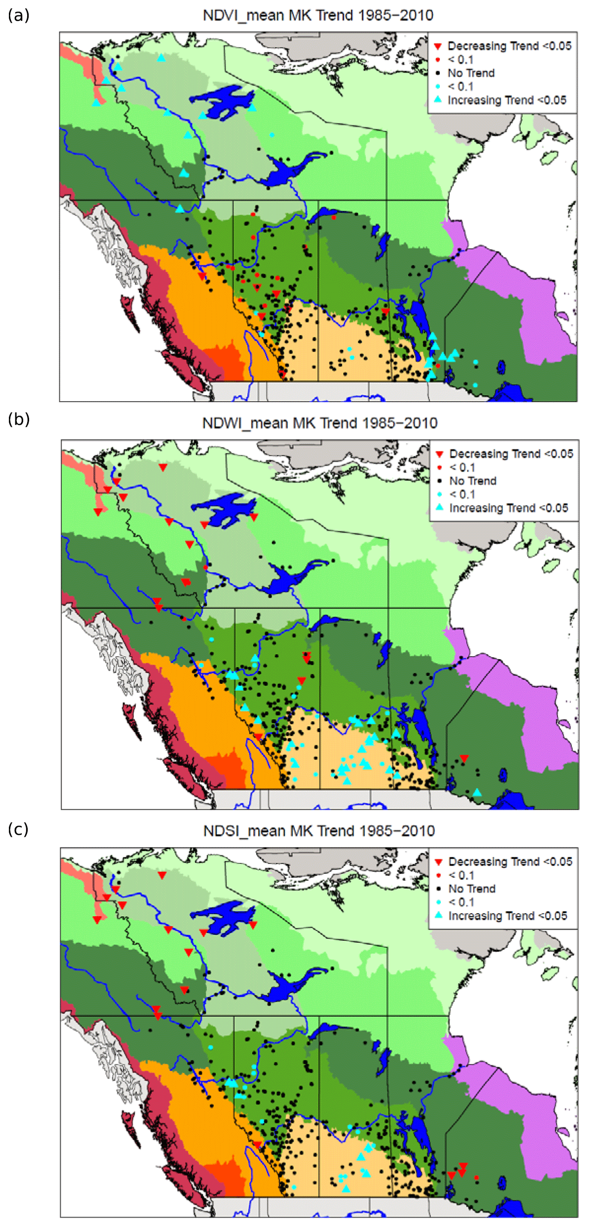
Figure 13 Trends in mean (a) NDVI, (b) NDWI, and (c) NDSI between 1985 and 2010. The ecozone legend is as in Fig. 7.

Table 7 Trends in satellite indices in relation to Streamflow Regime Type. The numbers are the fraction of stations showing a trend; values greater than 0.05 are in bold.

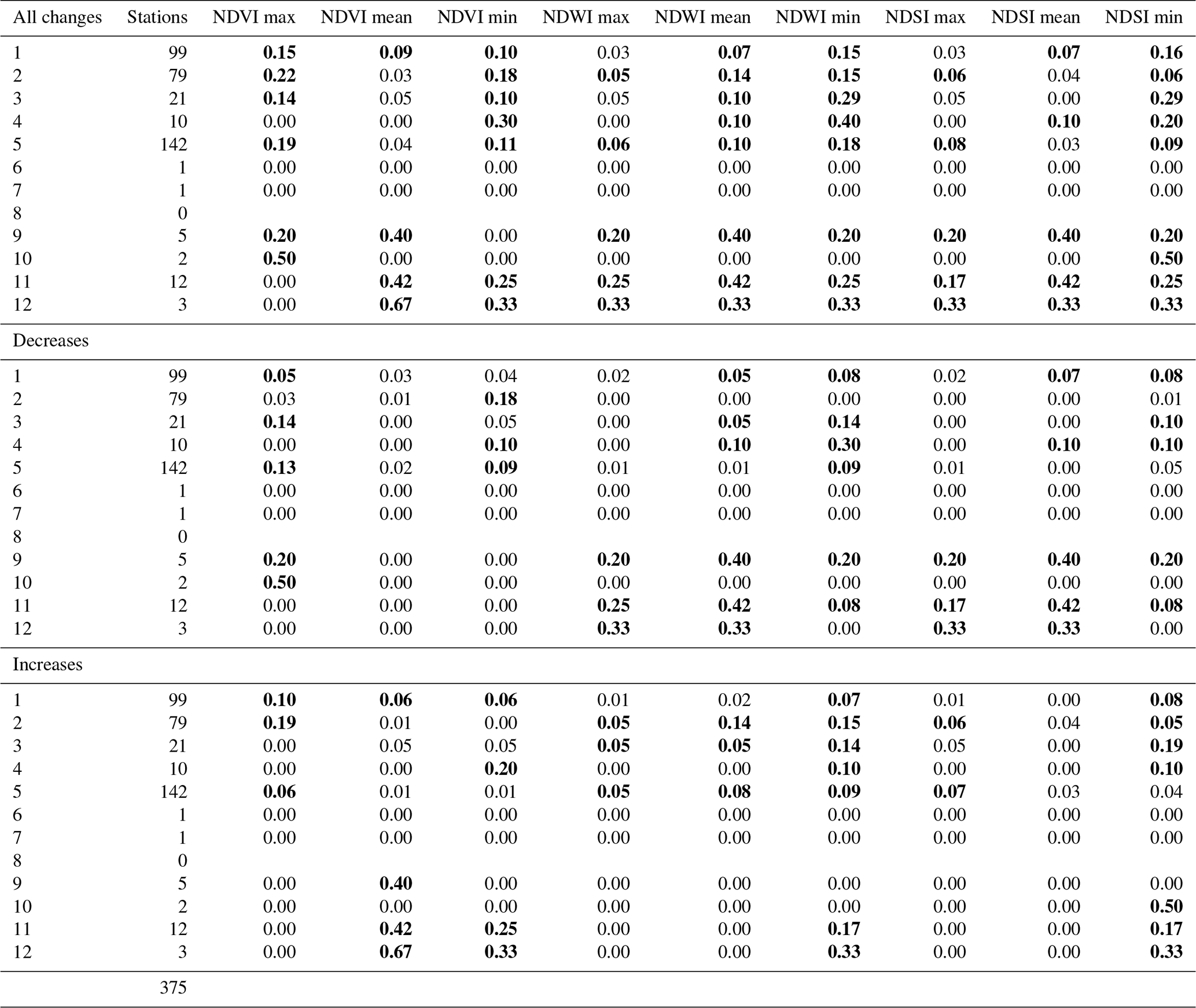
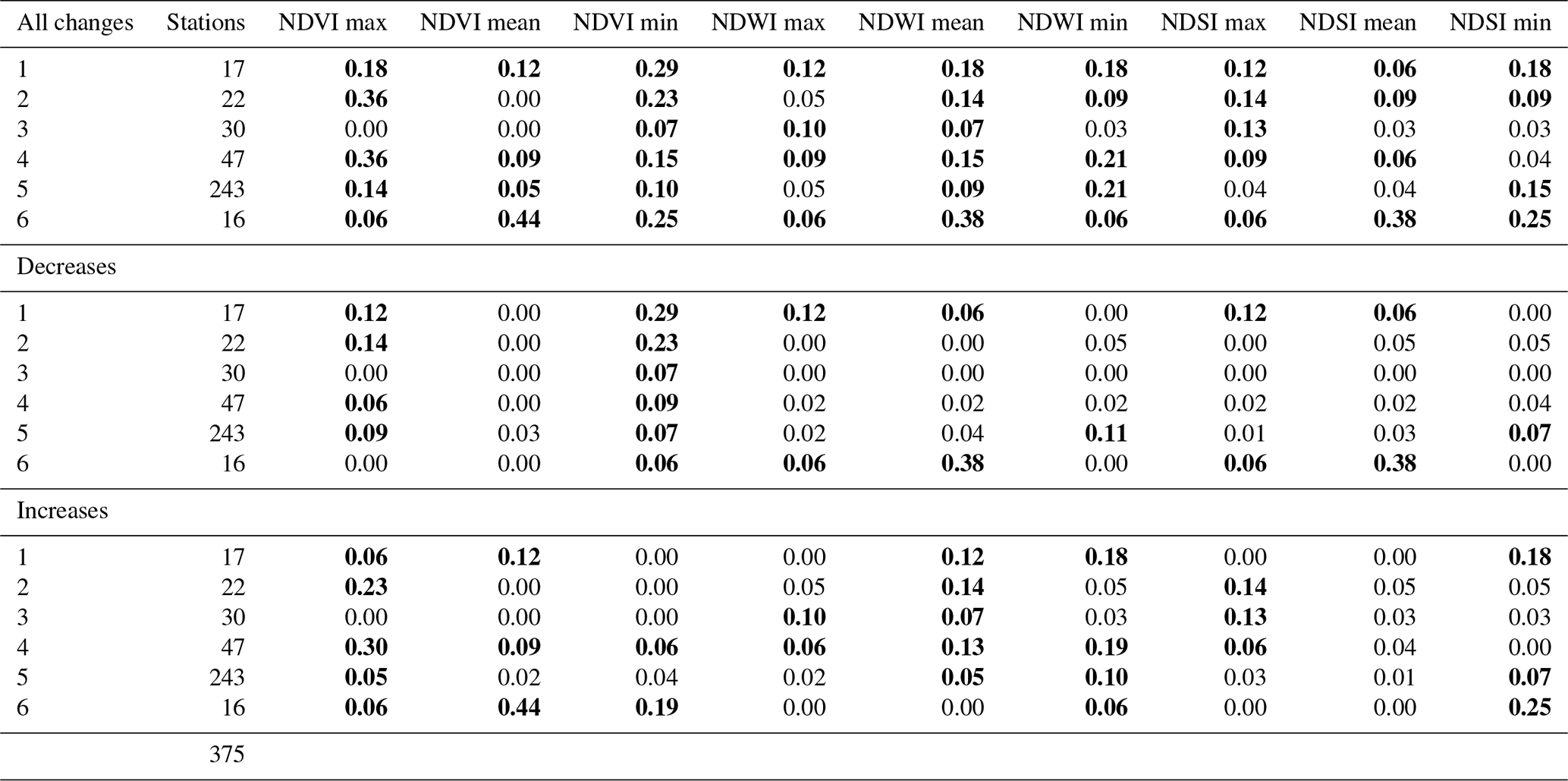
Table 8 Changes in satellite indices by Trend Pattern. The numbers are the fraction of stations showing a trend; values greater than 0.05 are in bold.

3.3.1 NDVI

The fractions of stations having statistically significant trends in NDVI were greater than the 5 % expected by chance alone for most Streamflow Regime Types, as listed in Table 7, which shows the combinations of increasing and decreasing trends and each trend separately. For example, the fraction of all significant trends for maximum NDVI exceeds 5 % in Streamflow Regime Types 1, 2, 3, 5, 9, and 10. The fraction of significant decreasing trends for maximum NDVI was greater than 5 % for Streamflow Regime Types 1, 3, 5, 9, and 10. The fraction of increasing trends in maximum NDVI exceeds 5 % in Streamflow Regime Types 1, 2, and 5. All significant trends in mean NDVI were increasing and occur in Streamflow Regime Types 1, 9, 11, and 12. Significant trends in minimum NDVI were predominantly decreasing in Streamflow Regime Types 2 and 5 and increasing in Streamflow Regime Types 1, 11, and 12 and both increasing and decreasing trends in Streamflow Regime Type 4.

There were also more significant trends in NDVI than would be expected by chance alone in all Trend Patterns (Table 8). The fraction of basins having significant trends in maximum NDVI exceeds 5 % in all Trend Patterns, except Trend Pattern 3, which had no basins with significant trends. All mean NDVI trends were increasing and occur only in Trend Patterns 1, 4, and 6. Minimum NDVI trends were predominantly decreasing in all six patterns and increasing in Trend Patterns 4 and 6.

The associations of trends in mean NDVI between 1985 and 2010 with ecozones are each shown in Figs. 13a and S22 and Table 9. There was a stronger association of NDVI trends with ecozones than with either Streamflow Regime Types or Trend Patterns. Increasing trends in mean NDVI occur in the Taiga Plains, Taiga Shield, Boreal Shield, Boreal Cordillera and Taiga Cordillera ecozones; decreasing trends in mean NDVI were found more often than expected by chance alone in the Montane Cordillera (Fig. 13a and Table 9). The spatial patterns of trends in mean NDVI were similar to those of the maximum and minimum NDVI (Fig. S23); however, there were more basins with significant trends in maximum and minimum NDVI than for mean NDVI. Basins with significant increasing trends in maximum NDVI were found in the western portion of the Prairies and in the Boreal Shield (Fig. S22a and Table 9); decreasing trends in maximum NDVI were found in the southern portion of the Boreal Plains, the eastern Prairies, and the southern Boreal Plains and Boreal Shield (Fig. S22a). The Taiga Plains has basins with both significant increasing and decreasing trends in minimum NDVI, and decreasing trends were found at greater than expected by change alone in the Taiga Shield, Boreal Plains, and Prairies (eastern); increasing trends were found in the Boreal Shield, Montane Cordillera, Boreal Cordillera, and Taiga Cordillera (Fig. S22c). Basins with significant trends were not randomly distributed through any ecozone, as spatial clustering was evident in each of the three NDVI trends in Fig. S22.

Table 9 Changes in satellite indices in relation to ecozones. The numbers are the fraction of stations showing a trend; values greater than 0.05 are in bold.

3.3.2 NDWI

There were more significant trends in NDWI (i.e. hydrological storage) than would be expected by chance alone in most Streamflow Regime Types (Table 7), and they were more prominent in the mean and minimum NDWI than in maximum NDWI. Significant trends in maximum NDWI exceed 5 % in Types 2, 5, 9, 11, and 12 with Streamflow Regime Types 9, 11, and 12 showing increasing trends much greater than the threshold (> 20 %), while Streamflow Regime Types 2, 3, and 5 show decreasing trends in about 5 % of the stations. Significant trends in mean NDWI include both decreasing trends in Streamflow Regime Types 1, 3, 4, 9, 11, and 12 and increasing trends in Streamflow Regime Types 2, 3, and 5. Significant trends in minimum NDWI were decreasing in Streamflow Regime Types 9 and 11 and increasing in Streamflow Regime Types 2 and 12, with both increasing and decreasing trends in Streamflow Regime Types 1, 3, 4, and 5. The largest fraction of significant trends (> 33 %) were decreasing trends in mean NDWI in Streamflow Regime Types 9, 11, and 12.

There were more significant trends in NDWI than would be expected by chance alone for all Trend Patterns (Table 8). Significant decreasing trends in maximum NDWI exceed the threshold 5 % in Trend Patterns 1 and 6, and increasing trends in Trend Patterns 3 and 4 (Table 8). Decreasing trends in mean NDWI exceed 5 % in Trend Patterns 1 and 6, as do increasing trends in Trend Patterns 1 to 5. The fraction of basins with decreasing trends in minimum NDWI exceeded 5 % in Trend Pattern 5 and for increasing trends in Trend Patterns 1, 4, 5, and 6. Only Trend Pattern 5, i.e. without a Trend Pattern, was found to have both increasing and decreasing trends in minimum NDWI.

The associations of trends in mean NDWI with ecozones are shown in Fig. 13b, and Table 9 (Fig. S23 shows results for maximum, mean, and minimum NDWI). Similar to NDVI, there was a stronger spatial association of NDWI trends with ecozones than with either Streamflow Regime Types or Trend Patterns. Decreasing trends in mean NDWI occur in the northern ecozones (Taiga Plains, Taiga Shield, Boreal Cordillera, and Taiga Cordillera; Figs. 13b and S23b); increasing trends in mean NDWI occur only in the Prairies and Boreal Plains. There were more significant trends in mean NDWI than in either maximum or minimum NDWI, but the spatial patterns for mean NDWI trends were similar to those for maximum and minimum NDWI. Basins with significant increasing trends in maximum NDWI were found only in the western portion of the Prairies and the Boreal Shield (Fig. S23a and Table 9); decreasing maximum NDWI trends were found in the eastern portion of the Boreal Plains and in the Cordillera (Fig. S23a). Both increasing and decreasing trends in minimum NDWI were found in the Taiga Plains, Boreal Shield, Boreal Plains, and Montane Cordillera (Fig. S23c). Only decreasing trends were found in the Taiga Shield and Hudson Plains, and increasing trends in minimum NDWI only occurred in the Prairies and Boreal Cordillera (Fig. S23c). Basins with significant trends were not randomly distributed through any ecozone, as spatial clustering was evident in each of the three NDWI trends in Fig. S23.

3.3.3 NDSI

There were also more significant trends in NDSI (snowcover) than would be expected by chance alone for all Streamflow Regime Types (Table 7); this was most prominent in the minimum NDSI. Significant decreasing trends in maximum NDSI exceed the 5 % of basins in Types 9, 11, and 12; increasing trends exceed 5 % in Types 2 and 5. Only decreasing trends in mean NDSI were detected in Streamflow Regime Types 1, 4, 9, 11, and 12. Both decreasing and increasing trends in minimum NDSI occurred in Streamflow Regime Types 1, 3, 4, and 11; in Streamflow Regime Type 9 only decreasing trends in minimum NDSI were found and only increasing trends in Types 2, 10, and 12. The fraction of stations showing increasing trends in minimum NDSI was much greater than that of decreasing trends.

There were more significant trends in NDSI than would be expected by chance alone for all streamflow Trend Patterns (Table 8), with increasing and decreasing trends having similar frequencies. The fraction of significant decreasing trends in maximum NDSI exceeds 5 % in Trend Patterns 1 and 6 (as was true for NDWI) and increasing trends in Trend Patterns 3, 4, and 5 (Table 8). No increasing trends were found in mean NDSI. Decreasing trends in maximum and mean NDSI exceed 5 % in Trend Patterns 1 and 6 and for minimum NDSI in Trend Pattern 5. Increasing trends in minimum NDSI occurred in Trend Patterns 1, 5, and 6. Only Trend Pattern 5, i.e. the pattern without a streamflow regime trend, was found to have both increasing and decreasing trends in minimum NDSI.

The associations of trends in NDSI with ecozones were shown in Figs. 13c and S24 and Table 9. As with NDVI and NDWI, there was a stronger association of NDWI trends with ecozones than with Streamflow Regime Types or Trend Patterns. Decreasing trends in mean NDSI occurred in the Taiga Plains, Taiga Shield, Boreal Shield, and Boreal Cordillera (Fig. 13c, Table 9); there were insignificant increasing trends in mean NDSI, but significant increases were evident in Fig. 13c in the Prairies and Boreal Plains. There were many more significant trends in minimum NDSI than in either maximum or mean NDSI (Table 9, Fig. S24). The spatial patterns for mean NDSI were similar to those for maximum and minimum NDSI. Basins with significant decreasing maximum NDSI trends were found in the Taiga Plains, Taiga Shield, and Boreal Cordillera (Fig. S24a, Table 9); decreasing maximum NDSI was found in the eastern portion of the Boreal Plains and in the Prairies. Trends in minimum NDSI were more numerous than for maximum or mean NDSI (Table 9) and include both increasing and decreasing trends in the Taiga Plains, Boreal Shield, and Boreal Plains (Fig. S24c). Only decreasing minimum NDSI trends were found in the Montane Cordillera, and increasing trends in minimum NDSI only occurred in the Prairies, Boreal Cordillera, and Taiga Cordillera. Basins with significant trends are not randomly distributed through any ecozone, as spatial clustering was evident in each of the three NDSI trends plotted in Fig. S24.

3.4 Trend patterns and changes in satellite indices

Trend Pattern 6 (Fig. S21), with prominent winter increases in streamflow across the permafrost-rich north (Taiga and Southern Arctic ecozones), was originally described by Whitfield and Cannon (2000). This region also has significant increases in mean NDVI (Fig. 13a) and decreases in mean NDWI and NDSI (Fig. 13b). At this scale, one interpretation of the observed trends would be that warming has altered the seasonal pattern and depth of frozen ground and has increased winter flows, groundwater connectivity, and also the greenness of these basins, which suggests increased evapotranspiration (Figs. 13a and S22) and has reduced both the amount of standing water (Figs. 13b and S23) and the snow-covered period (Figs. 13c and S24).

Three other increasing Trend Patterns (1, 2, and 4) show different temporal patterns of change. These three patterns were observed on the Prairies and southern Boreal Plains. These three Trend Patterns have considerable spatial overlap (Fig. 12).

Trend Pattern 1 (Fig. S16) was common in the Manitoba portion of the Prairie and Boreal Plains ecozone, with greater streamflows throughout the period when data were available. This region has no significant changes in mean NDVI (Fig. 13a), nor in NDSI (Fig. 13c), but there were increases in NDWI at the western edge of the region (Fig. 13b). One interpretation is that changes in vegetation and snow indices have been subtle. Streamflows have increased without altering the greenness (and hence evapotranspiration) of these basins (Figs. 13a and S22) or the snow-covered period (Figs. 13c and S24), but there has been increased wetness on the western side of this region (Figs. 13b and S23). The increase in storage is indicative of higher precipitation in this poorly drained post-glacial landscape.

Trend Pattern 2 (Fig. S17) was common in the Alberta and Saskatchewan portion of the Prairie and the Saskatchewan and Manitoba portion of the southern Boreal Plains ecozone. This region has no significant trends in mean NDVI (Fig. 13a) but does display significant positive trends in mean NDWI (Fig. 13b) and NDSI (Fig. 13c). An interpretation is that the increasing trend in water storage (Figs. 13b and S23) may be the result of increases in precipitation, and the increase in the snow-covered period may be due to increased snowfall, which through snowmelt runoff would also increase water storage (Figs. 13c and S24), but the greenness of these basins has not been altered (Figs. 13a and S22).

Trend Pattern 4 (Fig. S19) was common across the Prairie and southern Boreal Plains ecosystems. The region has no significant trends in mean NDVI (Fig. 13a) and only a few increasing trends in NDSI (Fig. 13c), which were restricted to Saskatchewan, but with significant increases in mean NDWI (Fig. 13b) except in Manitoba. Again here, the greenness of these basins has not changed (Figs. 13a and S22), despite trends in indices showing an increase in wetness (Figs. 13b and S23) which may be the result of increases in precipitation, and an increase in the snow-covered period which may be due to increased snowfall (Figs. 13c and S24).

Trend Pattern 3 (Fig. S18) was the only change pattern with decreasing streamflows and was common across the Prairie and southern Boreal Plains ecosystems. Decreasing trends in streamflow were more prevalent in the latter portion of the observed period. The region in which this pattern was observed is concentrated in the western part of the Boreal Plain and into the western portion of the Prairie ecosystem. This region has seen significant decreasing trends in mean NDVI (Fig. 13a), and the overlap of the areas with Trend Pattern 3 basins corresponds well to those basins demonstrating significantly decreasing mean NDVI and without trends in NDWI (Fig. 13b) or in mean NDSI (Fig. 13c). The greenness of these basins (Figs. 13a and S22) may have decreased because the basins are drier in summer since there are no decreases in wetness (Figs. 13b and S23) or snowcover (Figs. 13c and S24).

4 Discussion

This study set out to demonstrate an alternative approach to classifying streamflow regimes, to look for common seasonal Trend Patterns using a warm-season annual common time window across a large spatial domain, and to confirm or contrast hydrological changes with trends in satellite indices. The approach used here was targeted to assess those aspects that have changed and why, the basic element being the hydrological response that depends upon the key streamflow-generating processes in each basin. Analyses of change in this analysis were focused on seasonal patterns rather than on annual measures. In trend studies, time periods are selected that are a trade-off between record length and network density (Hannaford et al., 2013). Any fixed period of years may not be representative of historical variability (Hannaford et al., 2013). Given the large data sets, where stations have records for differing years, where gaps of years may exist in the streamflow record, and with a large number of basins that have only warm-season data, the results remain consistent over a wide range of period lengths of trend tests, with ∼80 % of results remaining unchanged, for periods greater than 30 years (Fig. 11). This suggests that the use of this unconventional methodology is entirely justified for trend studies, using record lengths greater than 30 years. Determining the magnitudes of trends in annual runoff or other annual attributes using this methodology is not appropriate.

By focusing on the warm-season annual common time window, the complex spatial structure seasonal pattern in flows and trends can be explored. In the large spatial domain of this study, it is essential that spatial linkages and patterns are considered for both Streamflow Regime Types and Trend Patterns. Using as many stations as possible, stations having continuous or seasonal operation, provides more resolution of the spatial extent of changes. Trends in streamflow due to climate or landscape changes are not expected to be spatially uniform (Carey et al., 2010; Patterson et al., 2012).

4.1 Streamflow Regime Types

Streamflow regimes are a useful way of considering seasonal hydrology (Bower et al., 2004). Unfortunately, the large numbers of standardized streamflows plotted in Fig. 6 make it difficult to compare the Streamflow Regime Types; plotting the z-score centroids of each (Fig. 8) makes the comparisons clearer. Each of the Streamflow Regime Type centroids have a dominant peak and a specific shape. The peaks may be narrow (Types 1 and 11) or broad (Types 3, 4, 9 and 12). Streamflow Regime Types 2 and 5 associated with the Prairies were not always sampled on the rising limb, because (a) the peaks are due to snowmelt, (b) the Prairies melt early in the year, and (c) the snowmelt period often occurs before the beginning of the annual common time window.

Sample hydrographs of individual stations from each type are shown in Figs. S2–S13. These similarities among the stations are due to the predominance of snowmelt as the source of streamflow in this cold region, and the differences are related to the combinations of landscape processes that mediate the melt (hypsometry, surface storage, groundwater, and glaciers). The classification produced by the algorithm is spatially reasonable in that stations from similar landscapes, hydrology, and climates were clustered together (Table 3). Stations which are nested along a single basin (e.g. Athabasca River, Type 3) were clustered together as the signal derived from the mountains propagates downstream. Distinctions between clusters draining differing terrains, which overlap spatially, such as at the boundary between the Cordillera and Prairies, are to be expected as the landscape gradients or differences are large. Similar results were found in Ontario (Razavi and Coulibaly, 2013). Three clusters (Streamflow Regime Types 6, 7, and 8) each contained a single member, and one (Type 10) had only two members. These Streamflow Regime Types are very different from those containing large numbers of members, and any clustering of hydrographs in this way must balance common characteristics against uniqueness. The use of DTW to address these issues in hydrology has been suggested previously (Ehret and Zehe, 2011; Ouyang et al., 2010; Mansor et al., 2018). Overall, the use of dynamic time warping overcomes the timing differences due to latitude and elevation. While median flows were used here because of the large number of stations, individual years could be used to develop a consensus clustering if a smaller number of stations were to be used.

4.2 Trend Patterns

Like the Streamflow Regime Types, the Trend Patterns also show strong spatial organization; one pattern of decreasing trends, four types of increasing trends, and a large group without trends (Table 5). There was no clear link between the Streamflow Regime Type and the Trend Pattern (Table 5). Basins in mountainous areas generally lack consistent patterns of trends (Trend Pattern 5), but some exceptions do occur. Many studies in British Columbia have shown late-summer streamflow declines (Leith and Whitfield, 1998; Jost et al., 2012; Fleming and Dahlke, 2014). This may be the result of hydrologic resilience (Harder et al., 2015) in mountain basins east of the Continental Divide.

The Trend Patterns have spatial distributions that appear to be unrelated to individual ecozones but, as would be expected from past descriptions of the predominant climate processes on the Prairies, drying in the west and wetting in the east (Borchert, 1950; Rosenberg, 1987; Luckman, 1990; Whitfield et al., 2020), and extending beyond any one ecozone. For example, over the Prairie ecozone (Fig. 12), there are three Trend Patterns with differing patterns of increasing streamflow. Trend Pattern 1 basins are located at the eastern and western margins of the Prairies in the partly forested “parkland” ecozone fringe (Figs. 12 and S16). Trend Pattern 2 basins are located across the Prairies but are concentrated in the more humid east and in the eastern portion of the forested Boreal Plains (Figs. 12 and S17). Trend Pattern 4 basins are scattered across the Prairies and occur along the southern margins of the Boreal Plains (Figs. 12 and S19). The decreasing Trend Pattern 3 basins are prominent in the foothills, boreal forest, and grassland regions just east of the Rocky Mountains across the Boreal Plains and just west of the Prairies (Fig. S18).

Although annual trends in climate and streamflow have been reported widely (e.g. Zhang et al., 2001; Peterson et al., 2002; Déry et al., 2009a; St. Jacques and Sauchyn, 2009; Shook and Pomeroy, 2012; Vincent et al., 2015, 2018), seasonal studies are less common, although they allow determination of process shifts at finer scales of analysis (Whitfield and Cannon 2000; Whitfield et al., 2002; Bennett et al., 2015; Auerbach et al., 2016). The focus of the present study was on runoff timing changes using methods originally developed by Leith and Whitfield (1998) and subsequent improvements (Déry et al., 2009b). Many of the changes reported here have been observed by others. Increased winter streamflow in northern Canada was reported by Whitfield and Cannon (2000) and others subsequently (St. Jacques and Sauchyn, 2009; Bawden et al., 2015). Timing shifts have been reported, particularly in the onset of the spring freshet (Burn, 1994; Westmacott and Burn, 1997) and smaller summer recessions (Leith and Whitfield, 1998). In the headwater basins of the Columbia River basin in British Columbia, the timing of spring snowmelt runoff only changed slightly, and summer flows were unchanged (Hatcher and Jones, 2013). The spatial extent of changes in basins on the Boreal Plains and Prairies are novel findings as studies in the past have seldom incorporated data from hydrometric stations with seasonal records. Using a classification of annual runoff patterns in streams across the Prairies and adjacent areas, Whitfield et al. (2020) determined that basins in the eastern portion of the Prairies were becoming wetter and basins in the west becoming drier, as would be expected (Borchert, 1950) and consistent with the increased streamflows reported for Smith Creek (Dumanski et al., 2015). But, no changes in precipitation or runoff of most seasonal and continuous streamflow records were detected in the Prairies (Ehsanzadeh et al., 2016). Several studies of precipitation in summer across the Prairies reflect similar pattern changes (Akinremi et al., 1999; Asong et al., 2016; DeBeer et al., 2016). In the US Great Plains, intensified drying and increased numbers and durations of low-flow periods and greater flow events of shorter duration were identified (Chatterjee et al., 2018).

The spatial clustering of Trend Patterns does not coincide with Streamflow Regime Types, or exactly with ecozones. The contiguous change regions are broad in space and span ecozone boundaries. This is indicative of changes that are taking place at scales different from those that generate runoff (Streamflow Regime Type) but are related to broad-scale changes that would be expected with changes in weather and climate patterns across the southern portion of the study area and with climate warming in the northern portion. These patterns were partially described by Whitfield and Cannon (2000), and they have been explored and reported on by others since (Burn and Hag Elnur, 2002; Woo and Thorne, 2003; Fleming, 2007; Janowicz, 2008; Bawden et al., 2015; Tan et al., 2018).

4.3 Trends in vegetation, water, and snow satellite indices

The primary interest in trends of normalized difference indices (NDVI, NDWI, and NDSI) was in determining whether the changes were driving or following observed streamflow Trend Patterns. Changes in land use and hydrology at the basin scale can drive streamflow regime changes (Fohrer et al., 2001; Woo et al., 2008). Satellite imagery is increasingly being used for basin-scale analysis, but these studies generally focus on a small number of cases in a small region (Coppin et al., 2004; Bevington et al., 2018; Soulard et al., 2016; Militino et al., 2018; Jorgenson et al., 2018; Lee et al., 2018).

The results presented here demonstrate several broad spatial patterns of change that warrant closer examination in the future. Four specific regions have results that demonstrate significant changes, or lack thereof, in hydrology and satellite indices. These four regions correspond to areas with changes in water storage reported in Rodell et al. (2018). These four GRACE trend regions are consistent with the results presented here. Rodell et al. (2018) suggested the regions result from the following mechanisms: (1) precipitation increases in northern Canada; (2) a progression from a dry to a wet period in the eastern Prairies/Great Plains; (3) a region of surface water drying in the eastern Boreal; and (4) a region of no change along the Rocky Mountains. Based on the results presented here, mechanisms different from those suggested by Rodell et al. (2018) should be considered.

4.3.1 North of 60^∘

Warming has increased winter flows (Figs. 10 and S21) (Whitfield et al., 2004) and increased the greenness of these basins (Figs. 13a and S22) and reduced both the amount of standing water (Figs. 13b and S23) and the snow-covered period (Figs. 13c and S24). Climate change is expected to affect Arctic hydrology by decreasing snowcover and snowfall, decreasing depths of soil freezing, increasing snow-free season rainfall, moving northward of the southern limit of permafrost, and causing an earlier snowmelt with more frequent ice lenses (Kane, 1997); however, it may also increase snowfall and snowcover in places (Krogh and Pomeroy, 2018). In northern Canada, regional and local hydrology are controlled by permafrost thaw (Kane, 1997; Woo et al., 2000; Whitfield and Cannon, 2000; Cannon and Whitfield, 2002; Janowicz, 2008; St. Jacques and Sauchyn, 2009), increasing surface and subsurface connectivity and increasing winter baseflow (Connon et al., 2014; Liljedahl et al., 2016; Carpino et al., 2018; Quinton et al., 2018). Annual runoff in the Mackenzie River has increasing trends due to increasing annual flow trends in the Liard and Peace rivers (Woo et al., 2000, 2008; Déry et al., 2009a; Rood et al., 2017).

Rodell et al. (2018) attributed the increasing trends in GRACE water storage in northern Canada to increased freshwater accumulations (e.g. Forman et al., 2012). Increasing trends in MODIS temperature and moisture patterns were more common than decreases (Potter and Crabtree, 2013). Changes in the timing and peaks of streamflow have occurred in snowmelt-dominated streams of Boreal Alaska, with increasing winter flows, freshet flows, and decreasing flows post-freshet similar to values observed here (Bennett et al., 2015). Climate-driven changes in one taiga/tundra basin include decreasing snowfall, sublimation, soil moisture and evapotranspiration, a deeper active layer, and an earlier loss of snowcover (Krogh and Pomeroy, 2018). The results presented here indicate increased streamflow, particularly in winter, and basin wetness in a wide region north of 60^∘; however, the total number of basins with data remains small.

4.3.2 The Boreal Plains

In the Boreal Plains, there has been more warming in winter and spring than in summer; none of the climate stations examined by Price et al. (2013) and Ireson et al. (2015) showed significant trends in annual precipitation over the interval 1950–2010, but some exhibited a significant decline in annual snowfall and snowfall fraction due to a shortened cold season and earlier snowmelt. In the western Boreal Plains there has been a pervasive decrease in warm-season streamflow (Figs. 10 and S18) accompanied by a decrease in the greenness of these basins (Figs. 13a and S22) because these basins are drier in summer, although satellite images do not show a change in water storage (Figs. 13b and S23) or snowcover (Figs. 13c and S24). The Boreal Plains are expected to be a region of strong ecological sensitivity under a changing climate (Ireson et al., 2015). The southern margins of the Aspen Parkland (a Prairie ecoregion) and Boreal followed the climatic moisture, suggesting that moisture supplies limit the southern extent of the forest (Hogg, 1994). The driest regions of the Boreal forest are found at low elevations in western–central Manitoba, across Saskatchewan and Alberta, and the southwestern Northwest Territories; the boundary follows the zero isoline of the water budget (precipitation minus potential evapotranspiration) (Hogg, 1994). These regions are drying, causing increased risks of forest fire (Groisman et al., 2004). The Boreal Plains are expected to become drier and to have increased frequencies of vegetation shifts and disturbances; forests are expected to contract in the north, while the southern margin will remain stationary (Ireson et al., 2015). Chronic moisture deficits are the controlling factor of the boundary between forest and grassland in Western Canada (Hogg, 1994). In the Boreal Plains, evapotranspiration and changes in soil storage dominate the water balance (Devito et al., 2005). Rodell et al. (2018) suggest that the decreasing trend in “central Canada” (actually, their region would be the western Boreal) was attributed to snowcover declines and to recent drying (Bouchard et al., 2013).

The subarctic climate of the Boreal region has large inter-annual variability and will be prone to future climate change (Woo et al., 2008). Models suggest that future winter flows will increase, spring snowmelt will advance, but that peak and summer flows will decline because evapotranspiration will have increased (Devito et al., 2005). The results presented here confirm these widespread drying trends in the western portion of the Boreal Plains.

4.3.3 The Prairies

Many studies of the Prairies published before 2010 showed drying trends, while more recent literature reports extensive wetting. The climate of the Prairies has become warmer and drier in the previous 50 years, and summer streamflows have decreased (Gan, 1998). More recent literature demonstrates recent increases in precipitation; e.g. Gerken et al. (2018) describe the increases in precipitation and decreases in temperature in the Canadian Prairies during summer, increasing both the probabilities of convection and atmospheric moisture. Garbrecht et al. (2004) report increasing trends in precipitation, streamflow, and evapotranspiration on the Great Plains where a 16 % increase in precipitation led to a 64 % increase in streamflow that occurred in fall, winter, and spring. The seasonality and timing of streamflow in the northern–central United States (Missouri, Souris-Red-Rainy, and Upper Mississippi basins) have changed; i.e. northern portions have earlier snowmelt peaks, and the probabilities of summer and fall streamflow peaks have increased (Ryberg et al., 2015). The number of days with snowfall and heavy snowfall has decreased in Western Canada and increased in the north (Vincent et al., 2018). The western Prairies (Mixed Grassland and Cypress Upland ecoregions) are becoming drier, while the northern and eastern portions (Aspen Parkland ecoregion) have increasing runoffs (Whitfield et al., 2020).

Three Trend Patterns (1, 2, and 4) show increasing streamflows with different temporal patterns of change (Figs. 10, S16, S17 and S20) and overlap the Prairies and southern Boreal Plains (Fig. 12). Change Pattern 1 basins (Fig. S16) are located in the eastern Prairies and the adjacent Boreal Plains and are accompanied by increases in NDVI and no changes in NDWI or NDSI. Change Pattern 2 (Fig. S17) is common in the Alberta and Saskatchewan portion of the Prairie and the Saskatchewan and Manitoba portion of the southern Boreal Plains ecozone and was accompanied by increases in NDWI and NDSI but not by changes in NDVI. Change Pattern 4 (Fig. S19) is also common over the Prairie and southern Boreal Plains ecosystems. This region also has few significant changes in mean NDVI (Fig. 13a) or NDSI (Fig. 13c) but shows increases in NDWI at the western edge of the region (Fig. 13b). These changes are complex and exhibit a series of changes in streamflow, greenness, and snowcover from east to west. In the Aspen Parkland ecoregion, the northern Prairie adjacent to the Boreal Plains has shown increased streamflows (Whitfield et al., 2020). The apparent wetting trend on the northern Great Plains was attributed to a drought that took place before GRACE was deployed followed by years with above-normal precipitation (Rodell et al., 2018).

The poorly drained, post-glacial drainage basins of the Prairie pothole region have high inter-annual variability of annual precipitation (Millett et al., 2009; Hayashi et al., 2016), and there has been oscillation on the decadal scale between wet and dry conditions (Winter and Rosenberry, 1998). A set of 16 closed-basin lakes in the Prairie pothole region that show long-term declining water levels over the 20th century provides a measure of the balance between precipitation and evaporation (van der Kamp et al., 2008). Since the 1990s the southern Prairie pothole region has been influenced by an extended period of increased wetness resulting in higher water levels (McKenna et al., 2017).

The 100th meridian divides North America into an arid west and a humid east, which is expressed in vegetation, hydrology, and agriculture (Seager et al., 2018a, b). This gradient arises from atmospheric circulation and the transport of moisture. In winter, regions west of the meridian are sheltered from Pacific storm precipitation; in summer a southerly flow moves air from the southwest and Gulf of Mexico northwards with a strong west–east moisture transport. Under increasing greenhouse gases the divide is expected to move eastward, resulting in spread of aridity (Seager et al., 2018b). The results presented here indicate that increasing wetness near the meridian is shifting westward in Canada.

4.3.4 The mountains

Most of the basins (73 %) in the Cordillera (Montane, Boreal, and Taiga) fall into Trend Pattern 5 (Table 6, Fig. S20), which has a general lack of structure in changes. Elevation becomes important to the pattern of climate change over western North America only when a significant continental-scale warming dominates, and it is not detectable in the early stages of climate change (Fyfe and Flato, 1999). The lack of trends or timing shifts despite dramatic climate change and decline in low-elevation snowpacks has been found at smaller scales such as Marmot Creek Research Basin in the Montane Cordillera of the central Canadian Rockies (Harder et al., 2015). Many of these basins show some periods with increases or decreases in flow consistent with freshet timing changes (e.g. Figs. 2 and 3), but there was a lack of consistency as indicated by the inability for a cluster of statistically similar patterns to be formed. These timing shifts have been widely reported (Leith and Whitfield, 1998; Luckman, 1998; Whitfield and Cannon, 2000; Rood and Samuelson, 2005; Forbes et al., 2011; Bennett et al., 2015; Luce, 2018; Philipsen et al., 2018; and others). Basins in these ecozones do have trends in NDVI, NDWI, and NDSI, but the results are mixed (Table 9). The fraction of basins with decreasing trends in mean NDVI only just exceeds the 5 % threshold in the Montane Cordillera (6 %); both mean NDWI and mean NDSI exceed the threshold in the Boreal Cordillera (25 %) and Taiga Cordillera (100 %). Increases in mean NDVI exceed the threshold in the Boreal Cordillera (25 %) and Taiga Cordillera (100 %), and there are no increasing trends in these three ecozones for either NDWI or NDSI, suggesting that changes are more prevalent in the north than in the south. Using a modelling approach (Bennett et al., 2012; Schnorbus et al., 2014) demonstrated that detecting climate-driven changes in basins in the British Columbia Rocky Mountains was difficult because of model uncertainty. Despite the ongoing deglaciation in the mountains of the west (Clarke et al., 2015), streamflows in basins in the Canadian Rockies can be resilient to changes in climate (Harder et al., 2015; Whitfield and Pomeroy, 2016).

4.4 Remaining questions, significance and future work

In the Arctic, the patterns, magnitudes, and mechanisms of hydrological and ecological change are often unpredictable or difficult to separate from other drivers (Hinzman et al., 2005). In many disciplines, understanding the complexity of the Arctic is challenged by a lack of scientific knowledge, observational and experimental time series, and the technical and logistic constraints of Arctic research. In the Boreal, Ireson et al. (2015) indicate that the current monitoring of climate, hydrology, and ecology are insufficient for understanding or predicting the potential responses to either human activities or a changing climate. Even with inclusion of more than 200 stations that are observed seasonally, there are regions in the study domain, particularly north of 60^∘, that have too few observations, and consequently the basins that are observed are often larger compared to those in southern regions.

It is important to note that climate signals, particularly for the Pacific Decadal Oscillation (PDO) and Arctic Oscillation (AO), were not considered here. Oscillation in the climate system can be manifest as tests on short time periods (Chen and Grasby, 2009; Hannaford et al., 2013). Bennett et al. (2015) showed some connections of streamflow in Boreal Alaska to PDO but not to AO. The interannual variability of the Liard River is correlated with the PDO (Rood et al., 2017). Within mountainous areas, such as the Cordillera, the hydrological response to the regional climate variability signal is likely to be modified by local factors including location, topography, and land characteristics (Thorne and Woo, 2011). Future work should consider adapting the methodology presented here to examining the relationships of streamflow to these climate signals (and others), by resampling the available station records including complete and partial-year streamflow records in relation to the climate indices.

Are landscape changes related to initial state, and are they a response to or a driver of hydrological change? Broad-scale studies examining streamflow trends and timing changes should employ multiple methods across different scales and consider regime-dependent shifts to better identify and understand changes (Bennett et al., 2015). Here, it was shown that there are several coincident and overlapping regions of change in streamflow and in satellite indices. Further studies, at a finer spatial scale, will be required to determine process drivers and responses.

The main premise of this study was to let the available data tell the story of hydrological structure and change in this large study domain. Including data from seasonal stations that only report a part of the year more than doubled the number of stations available for analysis, and most of these stations are located in the Prairie ecozone, which has often been omitted in studies because of the lack of continuous data. The structure of the available data is complicated, the data set contains streamflow records from entire years and/or only the warm season and for a variety of periods of years, and the sites are not evenly distributed across ecozones. Determining the magnitudes of annual trends was not appropriate with the approach used because of the inconsistency of years of data between sites. But, including the data from both seasonal and continuous stations and an annual common time window rather than only entire years, the results provide an interesting spatial story of trend direction. While there are timing shifts in many Cordillera basins, the changes are inconsistent between sites, suggesting a resilience to change in complex terrain as reported by Harder et al. (2015). In the north, winter streamflows are increasing, and these are reflected in changes detected in satellite indices. The western Boreal Plains basins exhibit decreasing trends in streamflow and are less green (NDVI). There was a complex pattern of changing streamflows across the Prairies, with some drying in the west and areas with different patterns of increased streamflow particularly in the northeastern Prairies.

The motivation for this study came from the NSERC Changing Cold Regions Network study of 2013–2018 (DeBeer et al., 2015, 2021) of Western Canada's rapidly changing cold interior. That study sought to integrate existing and new sources of data with improved predictive and observational tools to understand, diagnose, and predict interactions amongst the cryospheric, ecological, hydrological, and climatic components of this study area. The results presented here are already informing several science research agendas in Canada and internationally. The results also contribute to the Global Water Futures program of 2016–2023 (http://www.globalwaterfutures.ca, last access: 5 May 2021), which has an overarching goal of delivering risk management solutions to manage water futures in Canada in a time of unprecedented change.

The first step to managing future water changes is to understand those of the recent past and that are currently underway, and this study makes a strong contribution to that process. In particular, this study represents a step forward in addressing the complexity of hydrological change; there are many studies of individual basins which, when results are considered individually, tend to be more anecdotal than systematic. It is indeed simpler and easier when there are only a few cases to consider with common variables and record length, as in many studies, but with large numbers of basins the tools for dealing with significant changes are more limited. Sensitivity studies that assess the limits of partial-year analysis of hydrological structure and change are required and seem a logical next step.

5 Conclusions

This study uses accepted techniques with a very large data set to compare existing and new sources of data to understand and diagnose interactions amongst the climatic, hydrological, and ecological components of Western Canada's rapidly changing cold interior. Methods were used in a novel manner that treated hydrometric stations with only warm-season observations in the same way as continuously observed basins. A clustering methodology, dynamic time warping, overcomes differences in timing due to latitude or elevation, separated stations based on Streamflow Regime Type. A clustering of the seasonal pattern of streamflow regime change allowed the examination of the relationship of change with Streamflow Regime Types and with ecozones. Spatial location, rather than Streamflow Regime Type, was a strong determinant of change and was consistent with large-scale change in the climate system.

Trends in satellite indices (NDVI, NDWI, and NDSI), obtained from time series derived from Landsat observations, allow trends in these indices to be related to hydrological changes in nearly 400 basins. While there are no simple one-to-one correspondences among Streamflow Regime Types, seasonal pattern changes, and satellite indices, four prominent regions of changes were diagnosed; these regions were also identified by Rodell et al. (2018) to have changes in water storage as determined from GRACE satellites.

5.1 North of 60^∘

Increased streamflows, particularly in winter, are taking place in the northern portion of the Mackenzie Basin. In these basins, and in the general region, mean NDVI has not changed, but mean NDWI and NDSI have decreased. Degrading permafrost resulting in increased winter streamflow is an important change, which has been observed to take place in this region and which may be driving the observed changes in NDWI. Decreasing snowcover, evidenced by decreased NDSI, may be reflected in the shift in the partition of rainfall and snowfall due to warmer spring transition periods.

5.2 The Boreal Plains and the western Prairies

Decreased streamflows occur in these basins. In this area in general, mean NDVI has significantly decreased, but along the western margin mean NDWI and NDSI have increased. Decreased NDVI was consistent with decreased streamflow; as basins become drier, vegetation will be impacted. Increases in mean NDWI and NDSI occur only at the western margin of this region, suggesting a zone with complex gradients and changes.

5.3 The eastern Prairies

Increased streamflows in summer and fall are occurring across the Prairies, particularly in the east, and along the northern margin and the southern margin of the Boreal Plains. Three types of hydrological changes are evident with differing spatial locations, but the overlap between types suggests that there are multiple processes involved. In these basins, and in this area in general, mean NDVI has significantly increased, mean NDWI has increased, and mean NDSI has not changed. This is consistent with the higher rainfall ratio observed since the 1950s in the region, recent higher summer precipitation and both increased water storage and drainage reported in the northern and eastern Canadian Prairies. Basins in the eastern Prairie show increased streamflows through the entire period of the year that data are available. Some basins, which are centred in Saskatchewan, show increases only during summer and fall which are indicative of changes in the streamflow regime from nival towards pluvial. Some basins show only a narrow time of the year with increased streamflows, which was the largest of these three change patterns, and are found in the western Prairie and along the margin between the Prairie and Boreal Plains. In these basins, mean NDVI has not changed, but NDWI has increased in basins in Saskatchewan and Alberta, and mean NDSI has increased in Saskatchewan. These differences may reflect the differences in the three change patterns. The existence of the east-to-west gradient of these changes was predicted by previous climatological studies (Borchert, 1950; Rosenberg, 1987; Luckman, 1990).

5.4 The mountains

The mountain basins in this study appear to be resilient to change. These basins demonstrate several hydrograph types but generally lack structure in Trend Patterns. Individually, these basins do show periods with increases or decreases in streamflow consistent with freshet timing changes, as has been reported elsewhere, but there was sufficient inconsistency among the basins to define a specific pattern. Basins in these ecozones do have trends in NDVI, NDWI, and NDSI, but the results are mixed. There are decreasing trends in mean NDVI in the Montane Cordillera and mean NDWI and mean NDSI in the Boreal Cordillera and Taiga Cordillera and increasing trends in mean NDVI in the Boreal Cordillera and Taiga Cordillera, and there are no increasing trends in these three ecozones for either NDWI or NDSI; decreasing trends are more prevalent in the north than in the south.

The approach using an annual common time window presented here combines many more stations and years of data and increases the number of stations available for analysis quite dramatically from previous fixed time window methods. Analysis of only the annual common time window demonstrates groups with common spatial patterns in streamflow regimes and groups with common streamflow trends. A common annual time window in the warm season provides sufficient information to adequately resolve regional streamflow patterns and seasonal streamflow trends.