Characteristics of droughts in Argentina's core crop region

This study advances the understanding and impacts of dry episodes on wheat, corn, and soybean yields over Argentina's core crop region. The production of these major crops is intense and is the main contribution to the country's gross domestic product. Our analysis focuses on the droughts' properties, including their magnitude, frequency at different timescales, duration, and severity. We analyzed 40 years of precipitation and soil moisture anomalies and their corresponding nonparametric standardized indices at timescales of 1, 3, and 6 months. The climate variables were complemented with 40 years of the crops' yield data. The percentage of drought occurrence in northeastern Argentina ranges between 12 % and 18 %, with the larger values located towards the core crop region's eastern–northeastern sector. An analysis of drought duration suggests that most cases tend to occur for periods shorter than 3 months, while a few can extend up to 1 year, and even fewer can last longer. More importantly, regardless of the duration, droughts have larger impacts during the crops' critical growth period. Corn and soybean have their critical growth periods during summer and are more sensitive to precipitation and soil moisture deficits than wheat, which has its critical growth period during spring. Quantification of the relation between the droughts' indicators during the crops' critical periods and detrended annual crop yields was performed. Large drought severity values during the crop-sensitive months result in significant crop yield losses. Results suggest that shorter-scale indicators during sensitive periods are more appropriate for predicting crop yield losses than the longer-scale indicators. This new approach can be helpful for regional decision-making systems that support planning by water managers and agricultural stakeholders.

1 Introduction

Southeastern South America (SESA) is a region where agriculture and cattle ranching are the primary resources and contributors to its gross domestic product. In Argentina, for instance, exports of soybean, corn, and wheat and their derived products accounted for about USD 41.4 billion yearly, on average, for 2014–2018 (MAGyP, 2019). Most of the agriculture is rain fed, with irrigation accounting for less than 3 % of the total crop region (Siebert et al., 2013). Thus, crops and stockbreeding are susceptible to climate variability and extremes as they depend highly on natural rainfall. Corn is among the crops more sensitive to water deficits (Minetti et al., 2007), while soybean production requires a middle range of water availability and tends to be negatively impacted by either wet or dry seasonal extremes (Penalba et al., 2007).

Droughts may have devastating economic and social impacts. Documentation of individual drought events has shown that, indeed, this is the case. The 1988–1989 drought in Argentina was ranked as being among the worst episodes on record. The cultivated area was reduced by about 35 %, and the crop yield decreased by about 15 %, resulting in a 44 % loss in productivity and, consequently, high economic losses (IMF, 1990). Another severe drought episode took place during the 2003–2004 austral warm season. The drought started in September 2003 (austral spring), affecting river discharges. By April 2004, the lack of water in the Uruguay River led to the closure of 13 out of 14 turbines at the Salto Grande hydroelectric power plant (La Nación, 2004; Penalba and Vargas, 2008). Yet another severe episode took place during 2008–2009. This drought was, at the time, one of the most intense, with reductions in wheat yields of about 50 % and the death of 1.5 million head of cattle in Argentina (Barrionuevo, 2009). The drought of late 2011–2012 had substantial impacts on soybean and corn production, causing losses of the order of USD 2.5 billion (Webber, 2012). The more recent drought between November 2017 and April 2018 caused a drop of 33 % in soybean production and 15 % drop in maize production during the 2017–2018 season with respect to the previous year (MAGyP, 2018).

Statistical analyses of extreme events in SESA have shown that periods of water deficit can occur at different timescales, with an inverse relationship between frequency and duration, i.e., shorter-lived events tend to be more frequent than those of longer duration. Hence, many observational studies of drought have centered around two approaches. First, studies are based on monthly data to examine droughts' evolution at longer timescales. For instance, Minetti et al. (2007) showed that 1-month-long droughts account for about 53 % of all cases, 2-month droughts are present in 28 % of all cases, and droughts of 3 or more months represent less than 20 % of the cases. Second, studies with daily data have shown that even relatively short dry spells can significantly impact if they occur when crops are most sensitive to water availability, as is the case during the growing season. These dry spells occur over smaller regions than those observed in monthly data and, therefore, have a limited damaging effect (Naumann et al., 2008). Dry spell duration is about 6 d on average in the Humid Pampas, although they increase in length towards the west (Penalba and Llano, 2008; Llano and Penalba, 2010; Naumann et al., 2012). Longer dry spells also present an increasing gradient from east to west, with up to 60 d in the eastern sector and about 190 d in semi-arid west (Llano and Penalba, 2010).

Dry episodes in SESA have experienced decadal and longer time changes. Changes in the frequency of dry and wet spells were reported as early as in the 19th century by Ameghino (1884). He even proposed that such changes were due to the introduction of land use practices in colonial times, going back to the 17th century when water-retaining tall grass was replaced by short grass as agriculture started expanding. Recent studies (e.g., Barrucand et al., 2007; Vargas et al., 2011; Magrin et al., 2014) have reported that the frequency of dry events was larger during the first half of the 20th century but decreased during the second half when a notorious positive trend in precipitation favored the expansion of agriculture towards the west onto once semi-arid regions. Several studies have shown increases in monthly rainfall and a reduction in the number of dry spells during the 20th century (Penalba and Vargas, 2008; Naumann et al., 2008; Vargas et al., 2011). Interestingly, other recent studies (e.g., Krepper and Zucarelli, 2010; Chen et al., 2010; Lovino et al., 2014) have suggested that the positive trend in monthly precipitation may have slowed down in the first decade of the 21st Century. If confirmed, such change could be reflected in more droughts.

The cold phase of El Niño–Southern Oscillation (ENSO), i.e., La Niña, is widely recognized as an important forcing for the onset and duration of extreme dry periods in SESA (Labraga et al., 2002; Penalba and Vargas, 2004; Silvestri, 2005; Barrucand et al., 2007; Vargas et al., 2011). Yet, the ENSO cold phase forcing alone does not always lead to intense droughts (Chen et al., 2010; Cavalcanti, 2012). As discussed by Seager et al. (2010) and Mo and Berbery (2011), the ENSO signal on SESA droughts becomes more intense and with a better-defined spatial shape when the cold ENSO phase is concurrent with a warmer-than-average tropical North Atlantic. In addition to the remote forcings, regional and local factors may contribute to extreme event modulation once they are initiated (Mo and Schemm, 2008; Müller et al., 2014). The moisture transports and soil moisture conditions are all known to influence the events' duration and intensity. Not least, persistent atmospheric circulations, like those associated with blocking episodes, may hinder the development of precipitation systems during long periods. A documented case was the 1962 drought during which a persistent and intense blocking anticyclone prevented the supply of warm and moist air from Brazil and the Atlantic Ocean, leading to drought conditions over most of Argentina (Malaka and Nuñez, 1980).

This research aims to advance the understanding of dry episodes and the understanding of the impacts of dry episodes on wheat, corn, and soybean yields over Argentina's core crop region. Each crop has its phenology with different critical periods (when drought may significantly impact its growth). For this reason, it is essential to consider not only seasonal droughts but also those that center on the critical months. A drought climatology based on different indices is essential for identifying features that the analysis of a single index might miss. This is the approach followed here. Our documentation focuses on drought frequency, duration, and severity and assesses its impacts on the crop yields. Section 2 presents the region of interest and describes the data and methods. The results and productivity indices are shown in Sect. 3. Discussion and conclusions are presented in Sect. 4.

2 Methods

2.1 Region of interest

Our analysis focuses on SESA (Fig. 1a) and, more specifically, on the region known as the core crop region bounded by 36–29^∘ S and 65–59^∘ W (dark brown rectangle in Fig. 1b–d), where most (about 80 %) of the Argentine production of wheat, corn, and soybean are found. The dark green color points out the regions in which each crop's production is more intense. Values of production for each crop are also shown in Fig. 1b–d. This region includes, almost entirely, the provinces of Córdoba and Santa Fe and part of the provinces of Entre Ríos, Buenos Aires, La Pampa, Santiago del Estero, and Corrientes (provinces are identified in Fig. 1a).

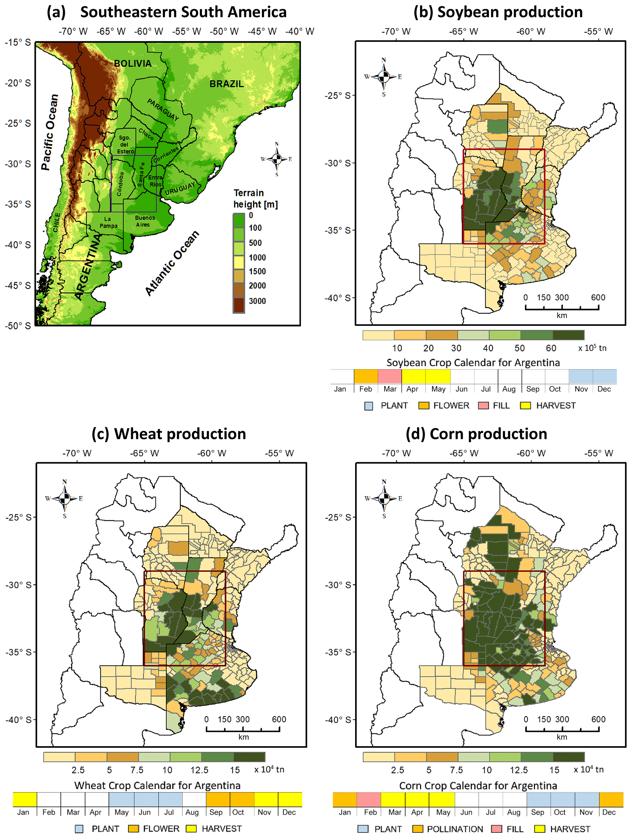
Figure 1 (a) Map of southern South America, with topographic levels and country names. The relevant Argentinian provinces are identified as well. Argentina's core crop region (highlighted with a dark brown rectangle) is the most productive region for corn, wheat, and soybean. The magnitude of production, in tonnes, was taken for the seasons 2010–2011 to 2017–2018 for soybean and corn and from 2010–2011 to 2018–2019 for wheat. The production magnitudes for soybean, wheat, and corn are presented in (b)–(d), respectively. The crops' development cycle is identified in the lower part of each panel. The periods of grain filling and flowering represent the most growth-sensitive months. They are October–November for wheat, December–January for corn, and January–February for soybean (MAGyP, 2019).

Wheat, corn, and soybean have different life cycles that last about 7 to 9 months (lower bars in Fig. 1b–d). Wheat is planted during late austral fall or early winter (May–June) and harvested during summer. It is most sensitive to water availability during its growth period in spring (October–November). Planting of corn and soybean occurs in austral spring (October–December), and both are harvested in the fall. Their most sensitive period takes place during the summer, specifically December–January for corn and January–February for soybeans. Therefore, a year's crop production could be largely impacted even if a dry period lasting just 1 month or even less occurs during the critical growth period. While these are the crops' traditional cycles, it has become possible to have double-cropping at specific locations, i.e., have two crops with different cycles in 1 year by making the second cycle shorter. Crop rotation – which also has the advantage of reducing the need for fertilizers – introduces the planting of corn or soybean right after the wheat harvest, and the second crop results in a smaller, but still profitable, production (Senigagliese, 2004).

2.2 Data sets and drought indices

This analysis of droughts focuses on precipitation (P), soil moisture (SM), and their derived standardized indices. Series of P and SM were turned into anomalies by removing their mean annual cycle. The monthly precipitation data cover 40 years, from January 1979 to December 2018, and were developed by the National Centers for Environmental Prediction (NCEP) Climate Prediction Center (CPC). It consists of in situ observations spatially interpolated to a regular $\mathrm{0.5}{}^{\circ }\times \mathrm{0.5}{}^{\circ }$ latitude–longitude grid cell (Chen et al., 2008). This product has been used as a benchmark for model evaluation in South America (Silva et al., 2011). In the absence of soil moisture observations, we employ products obtained from the Global Land Data Assimilation System (GLDAS; Rodell et al., 2004; Meng et al., 2012; Beaudoing and Rodell, 2019, 2020). GLDAS uses several land surface models to derive soil moisture from the surface water and energy balances forced by observations. The Noah model is considered here. It has four soil layers (0–10, 10–40, 40–100, and 100–200 cm) totaling 2 m depth (Rodell et al., 2004). The total soil moisture in a column is the sum of the content in the four layers. The soil moisture data set consists of monthly values at a spatial resolution of $\mathrm{0.25}{}^{\circ }\times \mathrm{0.25}{}^{\circ }$ over the same period of analysis as precipitation. Evaluation of GLDAS soil moisture products in the Humid Pampas was recently performed by Grings et al. (2015) and Spennemann et al. (2015, 2020). According to Grings et al. (2015), GLDAS is a good soil moisture benchmark in the Pampas region since it achieved the highest correlation (r>0.80) with in situ soil moisture measurements. Spennemann et al. (2015, 2020) also reported that GLDAS reproduces soil moisture observational patterns satisfactorily. They also found that GLDAS products can be used as soil monitoring indices in agricultural production management.

Several drought indices have been defined to characterize droughts. The World Meteorological Organization (WMO) recommends selecting a particular index, depending on the data available and ease of application (Byakatonda et al., 2018). It also recognizes the Standardized Precipitation Index (SPI) advantages for studying meteorological droughts (Hayes et al., 2011). SPI represents a standardized precipitation anomaly and stands among the most used indices to quantify and monitor droughts (Keyantash and Dracup, 2002; Mishra et al., 2009; Hayes et al., 2011). In addition to the SPI or any precipitation index, other environmental variables may need to be included, depending on the study region's characteristics and climate (e.g., Byakatonda et al., 2018). Soil moisture is particularly useful in agricultural areas, as they reflect the water content in the upper part of the soil where crops grow. Then, we used the SPI (McKee et al., 1993, 1995) for precipitation and the Standardized Soil Moisture Index (SSI; Hao and AghaKouchak, 2014; Hao et al., 2014) for soil moisture.

SPI and SSI were computed, following the approaches of Hao and AghaKouchak (2014) and Farahmand and AghaKouchak (2015), which allows us to obtain nonparametric standardized indices for precipitation and soil moisture. A growing body of research attests that a nonparametric approach is better than a parametric one for studies of droughts. Unlike parametric approaches, nonparametric methods do not rely on any theoretical distribution. Parametric and nonparametric (empirical) probability density functions tend to have differences in the tails, where the parametric distribution may not be a good fit (Farahmand and AghaKouchak, 2015). A comparison of parametric and nonparametric estimates of SPI (Soláková et al., 2014) found that differences can be significant in terms of drought severity and not as much in terms of duration. According to Mallenahalli (2020), the nonparametric SPI can better categorize the drought classes, representing the extent of dryness and normality conditions better than parametric approaches. For these reasons, we adopted a nonparametric methodology that uses an empirical function (Gringorten, 1963; Farahmand and AghaKouchak, 2015). This method circumvents the use of theoretical functions, avoids issues with zero precipitation values, and is suitable in precipitation and soil moisture studies. Moreover, it is also an opportunity to provide a different approach to the index construction that has not been tested yet in the region.

The SPI and SSI were calculated following a nonexceedance empirical probability function for extreme events (Gringorten, 1963).

$$\begin{array}{}\text{(1)}& p\left(x_i\right)={\displaystyle \frac{i-\mathrm{0.44}}{n+\mathrm{0.12}}}.\end{array}$$

Equation (1) represents the associated probability of nonexceedance for the ith element of the series, where x is either P or SM, i is the rank of nonzero values of the sample, and n is the size of the sample. This probability is then transformed into standardized indices (SIs), applying the inverse of the standard normal distribution function (∅) to the results of p(x_i) (Farahmand and AghaKouchak, 2015) as follows:

$$\begin{array}{}\text{(2)}& \mathrm{SI}={\mathrm{\varnothing }}^{-\mathrm{1}}\left(p\left(x_i\right)\right).\end{array}$$

This approach is applied to precipitation and soil moisture to create the corresponding indices of SPI and SSI.

Here, SPI and SSI are defined for two different timescales, 3 and 6 months, to facilitate the monitoring of meteorological and agricultural droughts. SPI3 (values for SPI at the 3-month scale) reflect wet or dry conditions for short and medium time ranges and estimate the climate conditions at critical stages of the crops' growth. SPI6 (values for SPI at the 6-month scale) provides information between seasons and can be a reference point for the start of the anomalous behavior of flows and reservoir levels, which usually have larger timescales than precipitation itself. As defined by soil moisture content, the less variable SSI index can identify and monitor seasonal agricultural droughts more directly (Hao et al., 2014). While SPI is widely used for drought monitoring and prediction, SSI produces a reliable representation of drought persistence (Farahmand and AghaKouchak, 2015). Additionally, we determined SPI1 (values for SPI at 1-month scale) as an index with higher variability for comparison in Figs. 2 and 4.

The time series of wheat, maize, and soybean yields cover the seasons from 1979–1980 to 2018–2019 for the provinces of Santa Fe and Córdoba, covering most of the core crop region (see Fig. 1d). Data are available from the Ministry of Agriculture, Livestock, and Fisheries (MAGyP, 2020).

2.3 Definitions and approach

A drought is a sustained period of below-normal water availability (Tallaksen and Van Lanen, 2004; Van Loon, 2015). Droughts are identified as being meteorological droughts when there is a precipitation deficit over a period of time. A continued precipitation deficit can lead to a scarcity of soil moisture that does not meet the plants' water demand. In this case, the drought is called an agricultural drought. This study focuses on meteorological and agricultural droughts and their impacts on crop yields within the region of interest.

For this analysis, droughts are defined as those periods in which SPI or SSI depart from the mean by at least minus 1 standard deviation. Drought events below that threshold range from moderate to extreme droughts (McKee et al., 1995). Weaker or milder droughts were estimated using a threshold of one-half the standard deviation. Droughts persist as long as they continue to exceed the threshold. We also examined different periods, starting at 1 month and continuing to more prolonged periods. We included the 1-month results in Fig. 6 for completeness, but most of our analysis and conclusions are based on longer periods.

Low-frequency variability modes in the drought indices were identified using a singular spectrum analysis (SSA) approach (Ghil et al., 2002; Wilks, 2006). SSA decomposes the time series in temporal–empirical orthogonal functions (T–EOFs) and temporal–principal components (T-PCs) and facilitates the interpretation of processes related to interannual modes of climate variability and the cases of drought. The SSA was used to identify the nonlinear trends and interannual quasi-oscillatory modes. Following Von Storch and Navarra (1995), we choose a window length (W) of 120 months, as it does not exceed one-third of the length of the whole period and resolves quasi-periods in the interannual band (1 year < T < 10 years).

Dry events were analyzed by studying their frequency, duration, severity, and areal extent. Drought frequency (F) indicates the percentage of droughts during the time of analysis, with respect to the total possible cases, in scales of months or the critical month periods for crop growth. Therefore, the frequency analysis is performed at monthly steps for the whole period and for each crop's critical period. The frequency distribution of drought events also depends on the duration (D); that is, the length in time that an index remains below the threshold until it reaches the threshold again. The drought magnitude is defined as the average deficit of an index during the duration of the event. The drought severity (S) is equivalent to the accumulated water deficit on the event (Dracup et al., 1980), and it is defined as the magnitude times the duration, i.e., $S=D\times M$ (see Yevjevich, 1967; Keyantash and Dracup, 2002). The properties of frequency, duration, and severity of droughts are unique to the thresholds that define them. The analysis is completed with the examination of the droughts' areal extent (A).

An analysis of the relation between drought occurrence and annual crop yields of wheat, corn, and soybean is performed for Santa Fe and Córdoba. First, crop yield data were detrended to remove the increasing yields resulting from technological and genetic improvements. The detrended series can be better related to drought characteristics. Then, we examined the Pearson correlation coefficients between the annual detrended crop yields and the drought indices for the critical crop months (October–November, ON, for wheat; December–January, DJ, for corn; January–February, JF, for soybean).

3 Results

3.1 Droughts in the core crop region

3.1.1 Spatial analysis

Figure 2 presents the spatial distribution of the percentage of months under moderate to extreme drought conditions for northern Argentina as characterized by SPI1, SPI3, SPI6, and soil moisture anomalies. The occurrence of drought in northeastern Argentina ranges between 12 % and 14 % for SPI1 (Fig. 2a), while months with droughts seem to increase up to 18 % as characterized by SPI3 and SPI6 (Fig. 2b and c). Soil moisture anomalies show that droughts are distributed mainly in the north of Argentina, with about 16 %–18 % of months with drought. Droughts, as characterized by SPI1, SPI3, and SPI6 (Fig. 2a–c), reveal a homogeneous spatial distribution and an increasing drought percentage, as with the timescale of the indicator. In contrast, the spatial pattern of soil moisture anomalies shows a decrease in drought percentages for arid regions (Fig. 2d). Inside the core crop region, droughts are more frequent towards the north, with percentages of months under moderate to extreme drought conditions from 14 % to 16 % for SPI1 and SPI3 (see Fig. 2a and b). Figure 2d indicates that months with drought conditions, as represented by SPI6, are equivalent to 18 % towards the region's north and southwest. Conversely, drought presence declines towards the southeastern core crop region, as all SPI and SM show percentages descending to 12 % (Fig. 2a–d).

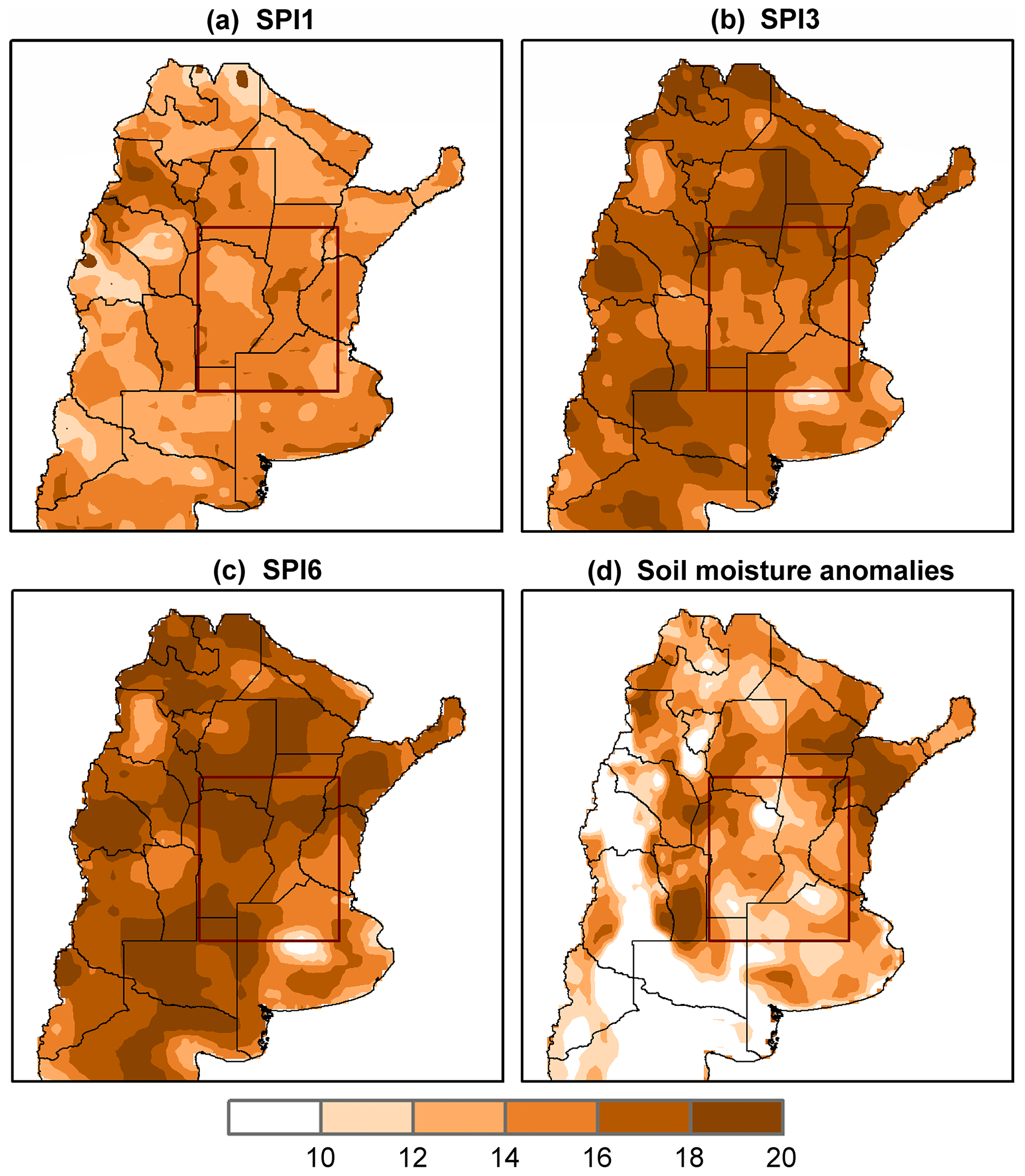
Figure 2 Percentage of months under moderate to extreme drought conditions (months below 1 standard deviation) of the total months, from January 1979 to December 2018, according to (a) SPI1, (b) SPI3, (c) SPI6, and (d) soil moisture anomalies.

The drought's occurrence during the crops' critical growing periods provides valuable information for decision-making. Crops have a stage during growth when they become more sensitive to water availability, and this changes with the type of crop. Spring and summer represent the most critical seasons in terms of the crops' critical months. For instance, the crucial period for wheat occurs in late spring (October and November). For corn, it is during the summer (December and January), and it is even later for soybean (January and February). Therefore, Fig. 3 presents the spatial distribution of the percentage of months under moderate to extreme drought conditions characterized by SPI during the corresponding critical months for each crop. The three crop types present many areas in which drought conditions are 18 % or higher. Figure 3a–c shows that shorter-duration droughts characterized by SPI3 tend to be more common towards the west of the region, particularly affecting corn and soybean crops. Figure 3d–f shows that longer duration droughts, as represented by SPI6, have a probability of 18 % over all of the core crop region but mainly during corn and soybean critical months. These results suggest that droughts over the core crop region are more frequent during summer months than during spring, affecting the corn and soybean critical periods more than the wheat's critical period.

Figure 3 Percentage of months under moderate to extreme drought conditions (months below 1 standard deviation) during the crops' critical growing months from January 1979 to December 2018. (a) Wheat during October–November, (b) corn during December–January, and (c) soybean during January–February for SPI3. Panels (d)–(f) are the same but for SPI6.

3.1.2 Temporal variability

Figure 4 presents the time series of SPI1, SPI3, SPI6, and soil moisture anomalies, area averaged over the core crop region. SPI indices and soil moisture (Fig. 4a–d) help identify wet and dry periods and their interannual variability. Notably, as the SPI timescale increases (from 1 month to 6 months), the variability is reduced (see Fig. 4a and c). Soils function as a physical filter because the output signal (soil moisture) has a lower frequency variability than the input precipitation. The reason is that the time it takes for the precipitated water to infiltrate the soil and move through deeper layers has a dampening or smoothing effect that Entekhabi et al. (1996) described as a low-pass filter.

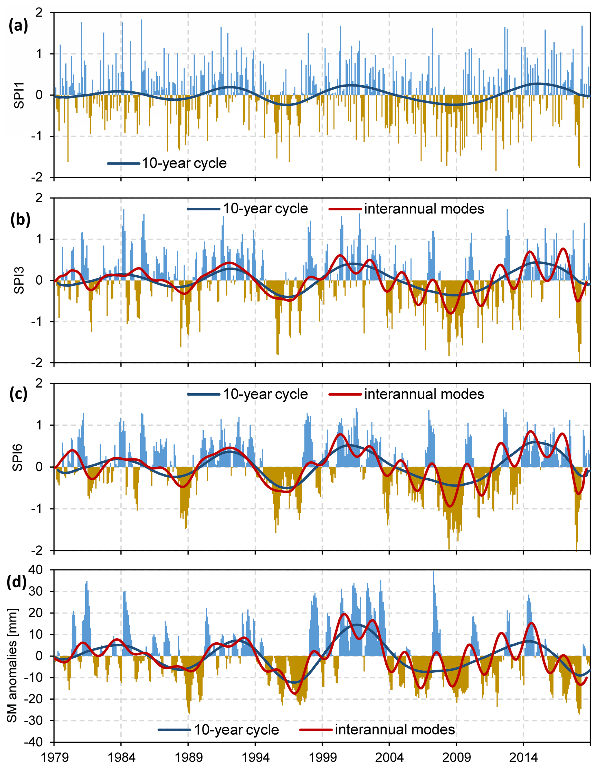
Figure 4 Areal-averaged time series from January 1979 to December 2018 for (a) SPI1, (b) SPI3, (c) SPI6, and (d) soil moisture anomalies in the core crop region. The dominant modes of interannual variability are plotted in solid lines.

Table 1 summarizes the dominant modes of interannual variability for SPI1, SPI3, SPI6, and soil moisture. They are (i) a trend, (ii) a band with decadal periodicities, and (iii) a band close to 2.3-year periodicities. Trends explain different percentages of the total variability of the series. Interannual modes in both bands can explain 35 % of the total variability of the SPI6 series and 37 % of the soil moisture variability. Decadal cycles in the SPI and soil moisture series are closely related and reflect the dry periods of 1987–1991, 1994–1999, and 2004–2013 (see Fig. 4a–d). The short-term 2.3-year cycle of interannual variability is evidenced by frequent wet and dry events between 2000 and 2018 (see Fig. 4b–d). Interestingly, higher amplitudes, starting around 2000, are noticed. This result agrees with Lovino et al. (2018a, b), who suggested that short-term variability (2.5- to 4-year periods) in precipitation exhibits a large increase in amplitude after 2000.

Table 1 Percentage of variance explained by the dominant modes of interannual variability detected, using SSA, with a window length of 120 months. Computations were done over SPI1, SPI3, SPI6, and soil moisture anomalies from January 1979 to December 2018 in the core crop region.

3.1.3 Frequency distribution

Figure 5 presents histograms of precipitation and soil moisture anomalies that were prepared to analyze the distribution of wet and dry periods over the core crop region. As we are dealing here with anomalies, a right-skewed histogram indicates more cases of water deficit conditions than water excess conditions, while a left-skewed histogram indicates the opposite. The kurtosis, in addition, reflects the propensity for producing outliers (Westfall, 2014). The precipitation and soil moisture anomalies display right-skewed histograms (Fig. 5a) with different kurtosis. This result indicates that drought episodes are more common than wet events over the region. The precipitation histogram (blue; hatched) exhibits extreme events that are related to a higher kurtosis (see inset in Fig. 5a) and heavy-tailed distribution (Westfall, 2014). The soil moisture histogram shows a more compact distribution, with low kurtosis and light-tailed histograms. This indicates that weak water deficit events are more frequent (e.g., about 150 events are found in the range −10 to 0 mm). On the other hand, a wider departure from the mean for the precipitation histogram indicates that extreme dry events may occur although their frequency is low, revealing, on the one hand, the need to use multiple indices and, on the other, the complexity of their simultaneous interpretation.

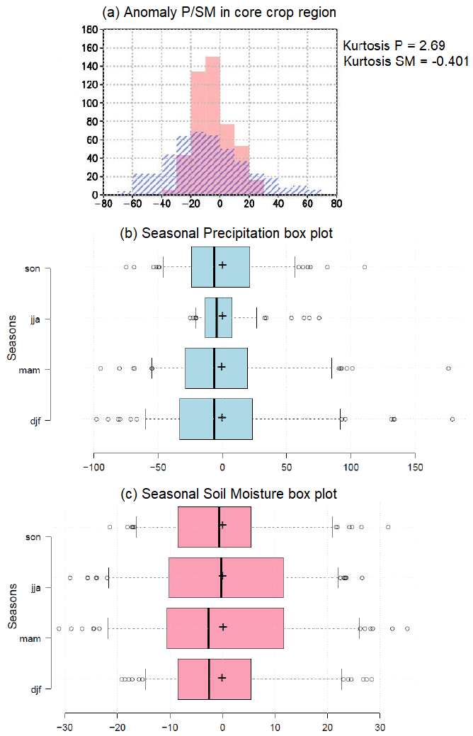
Figure 5 Frequency histograms in the core crop region and kurtosis values for (a) precipitation anomalies (blue; hatched) and soil moisture anomalies (light red). (b) Box plots of seasonally averaged time series inside the core crop region for precipitation anomalies. (c) Same as (b) but for soil moisture anomalies (light red). All computations were done from January 1979 to December 2018.

To better understand the seasonal distribution of dry events inside the core crop region, seasonal box plots were built for precipitation and soil moisture anomalies (Fig. 5b and c). The use of anomalies leads to an average of 0, while the median is slightly negative, following the skewed histograms in Fig. 5a. Precipitation plots in Fig. 5b present the widest distribution during summer (December–February; DJF), followed by autumn (March–May; MAM) and spring (September–November; SON). For each season, the lower and upper whiskers of the box plot stand for the 5th and 95th percentiles; values outside the whiskers (i.e., below the 5th percentile or above the 95th percentile) represent the outliers. The figure shows that the more extreme dry events can happen during summer and autumn, with outliers reaching −100 mm. In contrast, during winter (JJA), most of the values are found near 0 mm with small deviations. Outliers around −25 mm indicate that this region's events are not necessarily extreme.

Box plots for soil moisture in Fig. 5c show that seasonal distributions are more uniform, probably due to their lower variability and lower range values than precipitation. Interestingly, the outliers have the largest magnitudes during autumn (MAM), reaching deviations between −20 and −30 mm. This result is consistent with a delay with respect to precipitation, which showed the most extreme cases during summer (DJF). The delay also results in the soil moisture exhibiting more extreme cases during winter (JJA), following the large values for precipitation during autumn (MAM).

3.1.4 Drought duration

Drought duration is defined as the number of months that a given drought index (SPI and SSI) exceeds a certain threshold, X_i. For both SPI and SSI, the value $X_{\mathrm{1}}=-\mathrm{0.5}$ identifies mild to extreme droughts, while using $X_{\mathrm{2}}=-\mathrm{1}$ detects moderate to extreme droughts. Figure 6 shows the SPI and SSI frequency of droughts inside the core crop region regarding different events' durations, expressed in months. Each histogram presents the number of events for each duration, hinting at different types of droughts.

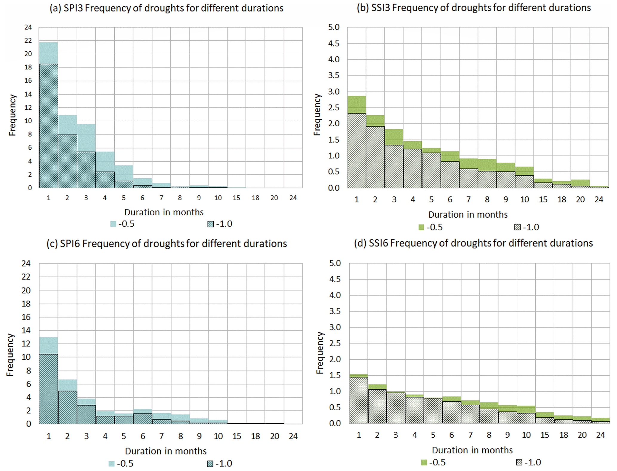
Figure 6 Histograms of droughts for different durations (in months) in the core crop region. (a) SPI3, (b) SSI3, (c) SPI6, and (d) SSI6. Color bars indicate mild to extreme droughts for which the values are less than $X_{\mathrm{1}}=-\mathrm{0.5}$. Hatched bars in all the panels indicate moderate to extreme droughts for which the values are less than $X_{\mathrm{2}}=-\mathrm{1}$. All computations were done from January 1979 to December 2018.

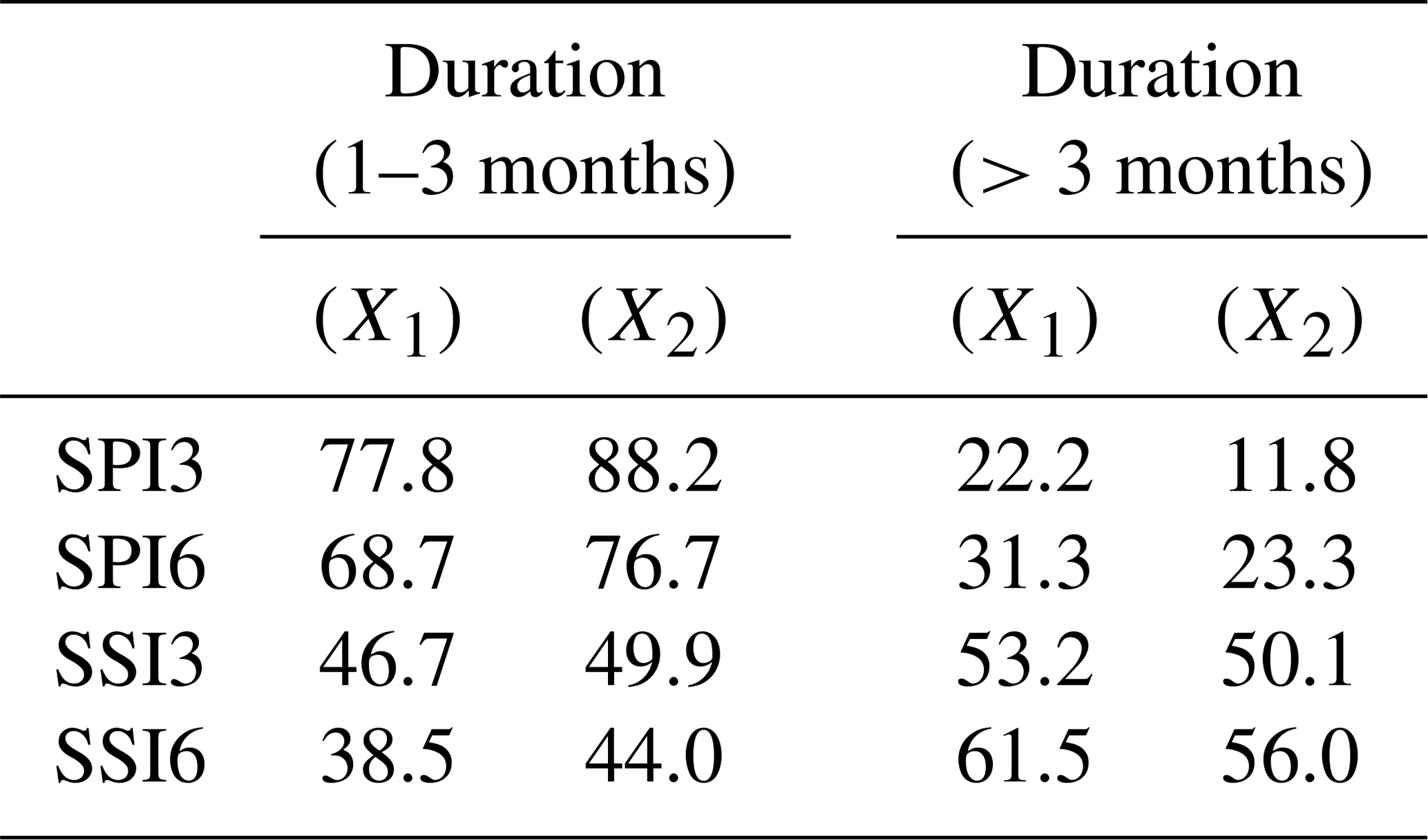
All histograms in Fig. 6 present a common pattern, with a higher frequency for short-term events (1–3 months). The frequency (or the number of cases) declines as drought duration increases. These results suggest that long-term droughts, particularly beyond 7 months, are uncommon in the core crop region. Table 2 presents the percentages of drought occurrence for short-term droughts and events more prolonged than 3 months, as characterized by SPIs and SSIs at timescales of 3 and 6 months. The SPI indices are better able to identify short-lived droughts than the standardized index based on soil moisture.

Table 2 Frequency of droughts for different durations, expressed as a percentage of the total drought events in core crop region, from indices of SPIs and SSIs. Droughts were detected using the thresholds X₁ (one-half standard deviation) and X₂ (one standard deviation) from January 1979 to December 2018. The duration of the events was grouped into short-term (1–3 months) and long-term droughts (>3 months).

In contrast, SSI seems a better fit to detect more prolonged droughts (see Table 2). In summary, short-term droughts are better represented by an index like SPI, with higher variability and a shorter timescale. Long-term drought events are more easily detected with an index of lower variability and a higher timescale.

3.1.5 Severity and spatial extent of droughts

Drought duration and magnitude are also essential for describing droughts. It is central to have a measure of severity and spatial extent of the drought. Severity can be defined as the product between the drought duration and drought magnitude. A drought's spatial extent refers to the area that exceeds a certain threshold (e.g., X₂), and it is expressed as a percentage of the total core crop region. Figure 7 presents the time series of severity and spatial extent, computed from SPIs and SSIs, for the core crop region. According to Fig. 7a and b, the most severe droughts occurred during 1988–1989, 1995–1996, 2008–2009, and the last one during 2017–2018, consistent with the analysis in Fig. 4. Time series of drought severity are negative because they result from the product of a negative drought magnitude (defined by using a negative threshold like X₂) and a positive duration. Severity indices seem to be greater in magnitude (more negative) when computed from 6-month timescales (SPI6 and SSI6), which is due to a lesser index variation as the time aggregation of the index increases.

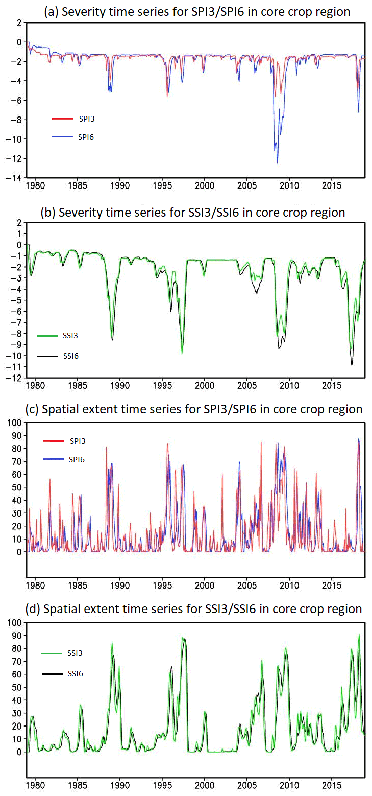
Figure 7 (a) Average time series of drought severity for events below X₂ in the core crop region based on SPI3 and SPI6 indices. (b) As in panel (a) but for SSI3 and SSI6. (c) Average time series of the droughts' spatial extent for events below X₂ as a percentage of the core crop region's total area, based on SPI3 and SPI6 indices. (d) As in panel (c) but for SSI3 and SSI6. All computations were done from January 1979 to December 2018.

The core crop region extends over 500 000 km² in Argentina's center (shown in Fig. 1). Figure 7a and c suggests that the more severe droughts are also the ones with a greater spatial extent within this area. Furthermore, for every severe event, the SPI time series indicate that droughts are extended around 80 % to 90 % of the core crop region, increasing these events' impacts on the region's main activities. Even droughts that are not quantitatively as severe can spread almost in equal proportions as the severe ones; for instance, the shorter droughts detected by SPI3 in 1996, 2002, 2006, and 2012 spread through 60 % to 80 % of the core crop region (see red lines in Fig. 7c). The soil moisture's lower variability results in similar time series of SSI3 and SSI6 (Fig. 7b and d) that have a high ability to identify drought events with increased severity and large spatial extension. Our results suggest that both SPI and SSI can identify severe droughts, but they have subtle differences. SPI is useful for detecting a drought's extension, whether it is severe or not. On the other hand, SSI tends to filter out nonsevere droughts, offering a cleaner representation of the more extended severe cases.

3.2 Crop yields in the core crop region

Due to the importance for regional economies, it is always of interest to stress the droughts' negative impact on crops. Changes in crop yield, defined as crop production per unit area, expressed as kilograms per hectare (kg ha⁻¹), reflect not only the effects of climate variability but also nonclimatic factors like technological and biotechnological advances (including seed quality, different use of fertilizers, and sawing or harvesting dates), usually in the form of a positive nonlinear trend. This can be seen in Fig. 8, which presents the 1979–2018 area-averaged time series of corn, wheat, and soybean yields for the provinces of Santa Fe and Córdoba. The wheat and soybean trends show a significant change around the mid-1990s, whereas, for corn, a change occurred earlier in the late 1980s. On average, wheat and soybean yields increased from 1000 to 3000 kg ha⁻¹ (Fig. 8a and c), while corn yield increased from 3000 to almost 8000 kg ha⁻¹ (Fig. 8b). As stated, at least most of the increases may be due to advances in the production process. These trends should be removed when examining the crop yield variability and its relation to droughts. Crop yield time series were fitted with a cubic polynomial trend (see dotted lines in Fig. 8a–c). Then, the trends were subtracted from the original series, leaving the shorter-term variability (see Fig. 8d–f). Detrended time series of one or more crop yields exhibit the largest negative anomalies concurrently with the most severe droughts identified by SPI6 and soil moisture anomalies (Fig. 4c and d) recorded in 1988–1989, 1995–1996, 2008–2009, and 2017–2018 (Fig. 8d–f). Not all crops are affected equally by drought, as slight differences in the onset of the drought and the crops' critical growth periods may affect them differently.

Figure 8 The time series of the area-averaged annual crop yield over the provinces of Santa Fe and Córdoba from 1979 to 2018. (a) Wheat, (b) corn, and (c) soybean yields. Cubic polynomial trends are shown as dotted lines. Panels (d)–(f) show the detrended yields for Santa Fe (blue) and Cordoba (orange). The superimposed gray bars characterize the SPI3 values corresponding to the crops' critical growing months, including ON for wheat, DJ for corn, and JF for soybean.

Table 3 presents the correlation coefficients between detrended crop yields and SPI/SSI during the crops' critical growth periods. The results suggest a direct relation between summer crops (corn and soybean) and deficits in precipitation and soil moisture during both crops' critical growth periods. Of the three crops, wheat yields have the lowest correlations with the indices. Table 3 also shows that the shorter-scale indicators (SPI3 and SSI3) achieve a better correlation with crop yields than the longer-scale indicators (SPI6 and SSI6), making them a good descriptor of crop yield losses.

Table 3 Correlation coefficients of the annual detrended crop yield and the maximum or minimum index value for critical crop months (ON for wheat, DJ for corn, and JF for soybean). Maximum or minimum index values are identified according to whether detrended annual crop yields are negative or positive.

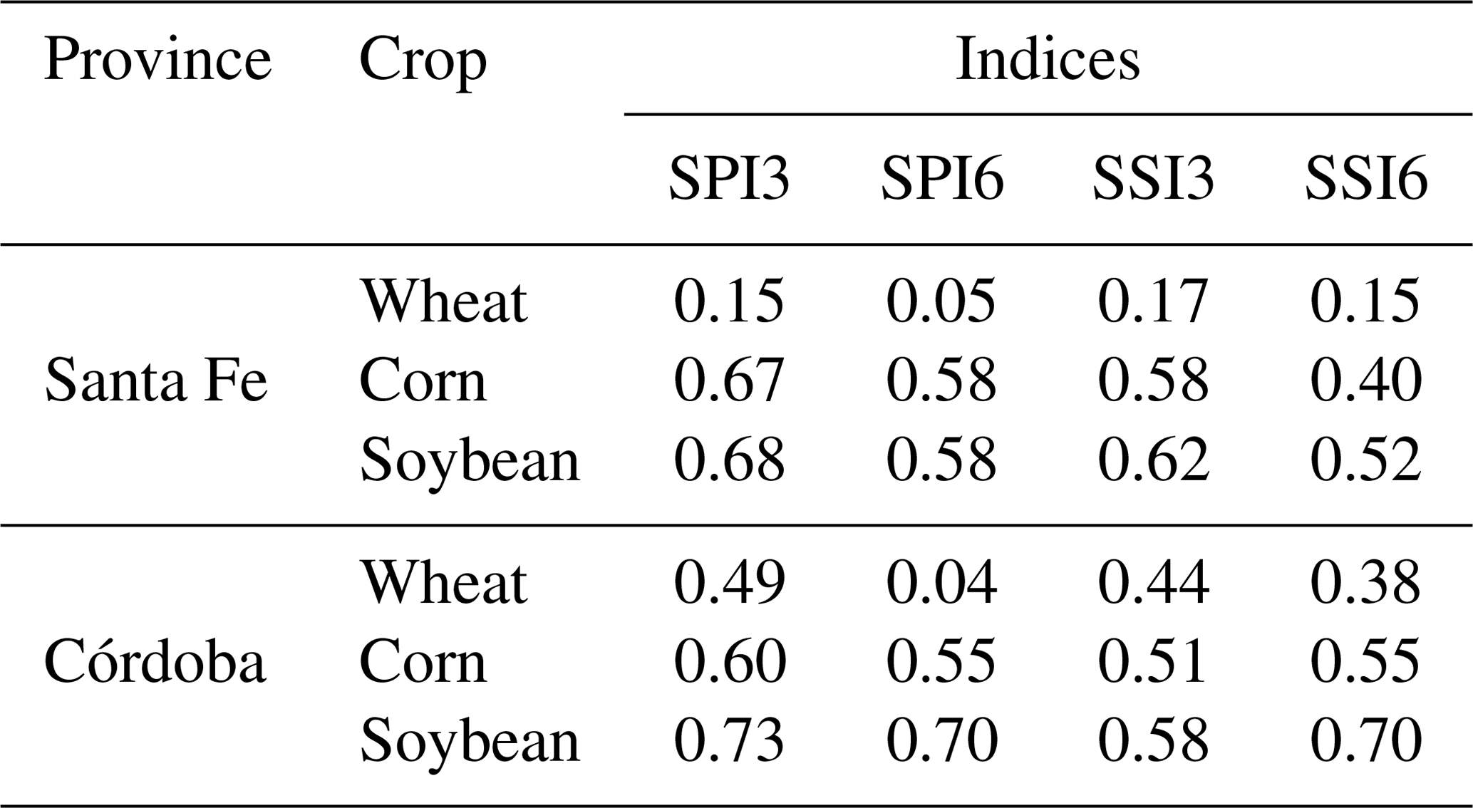
Figure 8d–f shows that large negative anomalies of detrended corn and soybean yields (Fig. 8e and f) are consistent with the lowest values of SPI3 during the drought events in 1988–1989, 1995–1996, and 2017–2018 (Fig. 7). Severity, derived from SSI3 and SSI6, reached extreme negative values around −8 during the crops' critical growth period. Similarly, a considerable reduction in wheat production in 2009 is related to large (negative) drought severity values, particularly for the Santa Fe province (see the blue line in Fig. 8d). Although there are some differences in the anomaly values, the detrended series of corn and soybean yield are in phase and exhibit a close resemblance (Fig. 8e and f). Increases and decreases in production take place nearly simultaneously, unlike the behavior of wheat (Fig. 8d). Both crops present significant yield losses approximately in the years of major droughts (see Fig. 7). This could be related to the 1-month overlap during both sensitive periods, as the two crops have January as a common month during their critical growth in the summer.

The detrended time series (Fig. 8d–f) show declines in production due to major drought events. The losses in production may reach up to 1500 kg ha⁻¹ for corn and between 500 and 1000 kg ha⁻¹ for wheat and soybean. Correlations between SPI3 and the different crop yields (Table 3) suggest that corn and soybean are more sensitive to water availability. Figure 8e and f show that SPI3 values and crop production have a better representation with a detrended series of corn and soybean yields. Notably, a good fit is observed for the most severe drought events in 1988–1989, 1995–1996, and 2017–2018. Conversely, from 1998 to 2007, no severe events occurred (see Fig. 7a and b). For those years, crop production ranges from neutral to positive values, with a maximum for corn in Córdoba. However, in this period without severe droughts, a drop in the Córdoba' soybean yield occurred in 2004 that is correlated with a moderate drought represented by an SPI close to −1.2 during the soybean's critical period. This could imply that SPI3 may also be used as a drought indicator during moderate drought events. We have not discussed the compound effect of water scarcity and heat waves, which may intensify crop yield losses. Llano and Vargas (2016) suggested that the compound event of precipitation and maximum temperature in the corn critical growth period have the greatest influences on crop production in central and eastern Argentina.

4 Discussion and conclusions

This study documents droughts in Argentina's core crop region, a region where wheat, corn, and soybean production is the most abundant. The investigation is based on the analysis of precipitation and soil moisture and their derived SPI and SSI indices, respectively, at different timescales. The drought properties that were examined include magnitude, duration, severity, and areal extension. The analysis was completed by examining the relationship between drought properties and crop yields. Droughts were identified as events with a water shortage exceeding 1 standard deviation, or more, of the mean values. The requirement was slightly relaxed for estimating the duration of events, considering water deficits that depart at least half of a standard deviation. The analysis was performed at different timescales, i.e., all months and monthly for each crop's critical growing months. Crop yields have increased through the years due to more beneficial climate conditions and, more importantly, thanks to agro-technological advancements. We inspected drought impacts on crop yield after removing those trends.

Our results indicate that the drought's occurrence percentage depends on whether SPI or SM anomalies are used, as the standardized nature and time aggregation of the SPI index tends to emphasize longer timescales. Short-term droughts are more easily detected when using an index with higher variability and a short timescale. For this reason, short-term drought-prone regions and their relation to seasonality within the core crop region are better identified using SPI1 and SPI3. The presence of long-term events is more readily recognized with an index of lower variability and at lower timescales.

Spatial patterns of drought's occurrence percentage for all times considered do not show clear features. The drought's occurrence percentage in northeastern Argentina ranges between 12 %–18 %, depending on the drought indicator and location, with the larger values found towards the core crop region's eastern–northeastern sector. The drought's percentage of occurrences, based on soil moisture anomalies, shows a second area of slightly high values for the semi-arid climate towards the core crop region's western portion. During summer, droughts affect corn and soybean production, mainly towards the west and center of the core crop region.

Soil moisture acts as a temporal filter because it smooths out the highly variable precipitation, resulting in a lower frequency signal. Similarly, the SPI time series variability is reduced when the timescale increases from 1 month to 6 months. Frequency analysis for different durations indicates that short-term droughts are more common than long-term droughts. Our findings show that values accumulated for 1–3 months account for about 78 %–88 % of the events, depending on the threshold and variable considered. A few can extend up to 1 year and even fewer last even longer. However, if a multiyear drought experienced breaks, each period would be regarded as a separate case. These results are consistent with drought frequency values found by Minetti et al. (2007), who reported that similar 1–3 months events account for 90 % of the Argentine Humid Pampa cases. Small differences could be related to the use of different indices and thresholds in the definition of drought. In general, long-term drought events are more easily detected with an index of lower variability, like SSI, and a higher timescale.

The timing of droughts is central to their impact on crop yields. The reason is that the crops' fastest growth during the critical periods is highly susceptible to water availability. Even a short-duration dry event, if concurrent with the critical growth period, may significantly impact crop performance. Large drought severity values taking place during sensitive months will result in significant crop yield losses. Suppose a severe drought event is identified and quantified during the crop-sensitive months. In that case, the drought indicator can be helpful as a warning that crop yields can be expected to be lower, potentially resulting in significant economic losses. Our results suggest that the shorter-scale indicators (SPI3 and SSI3) during crop critical periods are most appropriate for predicting crop yield losses than the longer-scale indicators (SPI6 and SSI6).

Argentine agriculture has benefited from the increased use of fertilizers, agrochemicals, and the management of genetically modified crops, leading to important positive trends in crop yields. Removing those trends facilitates contrasting of year-to-year yield variability and climate variations. Previous studies have partially addressed the relationship between droughts and losses on crop yields (e.g., Podestá et al., 2009; Holzman et al., 2014; Jozami et al., 2018). Our study advances the topic by providing a novel severity analysis and quantifying the link between detrended crop yield and drought indicators (SPI/SSI) during crop critical growth periods. Wheat yields have the lowest correlations with drought indices. On the other hand, our results suggest a direct relation between corn and soybean yields and deficits in precipitation and soil moisture during both crops' critical growth periods. Corn seems to be the summer crop most sensitive to water deficits, in terms of crop productivity. As a note of caution, corn production may be affected by water availability and temperature and geographical adaptation (Butler and Huybers, 2013). These two features have not been addressed here.