A simple cloud-filling approach for remote sensing water cover assessments

The empirical attribution of hydrologic change presents a unique data availability challenge in terms of establishing baseline prior conditions, as one cannot go back in time to retrospectively collect the necessary data. Although global remote sensing data can alleviate this challenge, most satellite missions are too recent to capture changes that happened long ago enough to provide sufficient observations for adequate statistical inference. In that context, the 4 decades of continuous global high-resolution monitoring enabled by the Landsat missions are an unrivaled source of information. However, constructing a time series of land cover observation across Landsat missions remains a significant challenge because cloud masking and inconsistent image quality complicate the automatized interpretation of optical imagery.

Focusing on the monitoring of lake water extent, we present an automatized gap-filling approach to infer the class (wet or dry) of pixels masked by clouds or sensing errors. The classification outcome of unmasked pixels is compiled across images taken on different dates to estimate the inundation frequency of each pixel, based on the assumption that different pixels are masked at different times. The inundation frequency is then used to infer the inundation status of masked pixels on individual images through supervised classification. Applied to a variety of global lakes with substantial long term or seasonal fluctuations, the approach successfully captured water extent variations obtained from in situ gauges (where applicable), or from other Landsat missions during overlapping time periods. Although sensitive to classification errors in the input imagery, the gap-filling algorithm is straightforward to implement on Google's Earth Engine platform and stands as a scalable approach to reliably monitor, and ultimately attribute, historical changes in water bodies.

1 Introduction

The water extent of many lakes has changed substantially over the last few decades (Busker et al., 2019). Once imposing bodies of water have declined to a small fraction of their historical volume in many parts of the world, with the Aral Sea standing out as an iconic example (Micklin, 2007). In more humid climates, shifts in the flow regimes of tributary streams has affected the seasonal variability in the corresponding lakes. For example, in the Mekong basin, changes in the seasonal flood pulse of the Tonlé Sap threaten the lake's sensitive ecosystems and fishery (Kummu and Sarkkula, 2008), with direct repercussions for the region's food security and unique biodiversity. These changes often emerge as a result of the complex interplay of natural (e.g., changing temperatures and precipitations) and anthropogenic (damming and irrigation) factors (Haddeland et al., 2014). Proper attribution of their drivers is critical to inform policy, but it is hampered by a dearth of monitoring data due to prevailing financial, institutional, and legal barriers (Solander et al., 2016). In that context, a substantial body of recent research has focused on monitoring surface water extents using satellite data, with applications ranging from small reservoirs (Avisse et al., 2017; Gao et al., 2012; Zhao and Gao, 2018) to large water bodies (Mercier et al., 2002) at the regional (Müller et al., 2016), continental (Zou et al., 2018), and global scales (Busker et al., 2019; Pekel et al., 2016a; Gao et al., 2012; Wang et al., 2018). By providing a consistent global space–time representation of the Earth system, satellite imagery offers a unique ability to study and attribute change ex post, in situations where in situ observations are nonexistent, unavailable, or disputed. Yet a sufficiently large sample of high-quality remote sensing observations is necessary to attribute change with adequate statistical power (Müller and Levy, 2019). Hence, imagery used to monitor lake water extent to quantify long-term patterns needs to (i) cover a sufficiently long period of regular observations (e.g., several decades of monthly observations) and (ii) allow open water to be consistently distinguished from dry land at a high spatial resolution in all weather conditions, including through clouds. These two requirements are challenging to satisfy simultaneously.

All-weather water detection can be achieved using active remote sensing at microwave frequencies. The process is unimpeded by clouds and does not rely on reflected sunlight. Synthetic aperture radars (SARs), in particular, leverage the fact that areas of open, smooth water bodies exhibit lower backscatter coefficients in the X, L, or C bands (Bioresita et al., 2018). A number of recently launched SAR missions (e.g., COSMO-SkyMed, TerraSAR-X, and Sentinel-1) allow for the detection of water at resolutions and return times that are appropriate for capturing local changes in water cover (Pérez Valentín and Müller, 2020). For instance, Sentinel-1 was launched in 2014 and has a 6 d revisit time and a spatial resolution of 20 m. However promising in their ability to monitor ongoing changes, these very recent sensors are unable to capture events that happened before their launch.

In contrast, satellites with optical sensors have been orbiting the Earth for decades and remain a preferred source of information to monitor open water (see Huang et al., 2018a, for a recent review). A number of spectral indices have been proposed to detect water using multispectral imagery (see Zhou et al., 2017), including the Modified Normalized Difference Water Index (MNDWI; Xu, 2006) used in this study. These indices leverage the high contrast between land and water at specific frequencies of the electromagnetic spectrum, and a range of techniques have been developed to systematically classify pixels as “wet” or “dry”, based on their spectral index (see Lu and Weng, 2007). A fundamental limitation of optical sensors, however, is their inability to capture land surface reflectance through clouds. A number of studies have addressed this impediment by leveraging the high (daily) return time of NASA's Moderate Resolution Imaging Spectroradiometer (MODIS) mission to build cloud-free, lower frequency (e.g., bi-weekly) mosaics (Gao et al., 2012; Wang et al., 2018). MODIS has relatively short coverage period (1999 and 2002 to the present for the Terra and Aqua satellites, respectively) but has been combined with space-borne radar altimeters to monitor lake water extents in earlier periods (up to 1992, using the Topex–Poseidon altimeter) by leveraging overlapping coverage periods to estimate water level–inundation area relationships (Gao et al., 2012). However, the limitations normally associated with radar altimetry (narrow swath, coarse cross-track spacing, and large along-track path length (see Yale et al., 1998) have restricted this approach to lakes that are well covered by altimeter orbits (Gao et al., 2012). In addition, the relatively coarse spatial resolution (250 to 500 m for visible and near-infrared bands) of MODIS limits its applicability for smaller lakes. Unlike MODIS, the successive Landsat missions provide high-resolution coverage of the Earth's surface since the 1970s. Landsat imagery has recently been used by Pekel et al. (2016a) to generate consistent monthly 30 m resolution estimates of global surface water cover (GSW) between the mid-1980s and 2015. However, Landsat image interpretation is complicated by a set of well-known challenges including clouds, cloud shadows, terrain shadows, and the Scan Line Corrector (SLC) failure on Landsat 7. These effects complicate the detection of surface water, causing approximately one-third of the pixels in the GSW data set to be marked as “no data” (see the code and data availability section). Discarding these masked pixels when identifying water-covered pixels will lead to a substantial underestimation of water cover (Zhao and Gao, 2018). This points to the need for scalable and easily implementable post-processing approaches to infer the inundation status of masked pixels.

We address this problem by predicting the binary class (e.g., wet or dry) of masked (no data) pixels, based on the observed class of comparable unmasked pixels. A total of two broad sets of such gap-filling approaches have been proposed in the literature. The first set of approaches is based on topographic consistency, i.e., a pixel will not be dry if it lies at an elevation that is lower than the highest (unmasked) “inundated” pixel within the same water body (Khandelwal et al., 2017; Avisse et al., 2017). An important limitation to these approaches is the reliance on either a digital elevation model (Khandelwal et al., 2017; Avisse et al., 2017) or a radar altimeter (Van Den Hoek et al., 2019). However, digital elevation models can have a low level of accuracy in the vertical direction (with standard deviation of the order of meters; Avisse et al., 2017) and may not capture the topography of regions that were flooded during the satellite overpass, whereas radar altimeters are limited with the spatial coverage limitations that we previously discussed (Yale et al., 1998). In contrast, the second set of studies does not rely on ancillary information but uses the historical inundation frequency (IF) of a masked pixel (estimated using observations taken at times when the pixel was unmasked) to predict its current inundation status. Zou et al. (2018) use a fixed IF threshold of 0.75 (i.e., pixels that are inundated on 75 % or more of the unmasked images) to identify permanent water bodies. Zhao and Gao (2018) apply a heuristic on the histogram of the IF of unmasked inundated pixels; masked pixels with an IF value larger than the IF corresponding to an arbitrary (i.e., 0.17) fraction of the mean histogram value are classified as inundated. Schwatke et al. (2019) use an IF image as a proxy for a digital elevation model and estimates an area–IF curve for each lake as a proxy for its area–elevation curve. An iterative algorithm is then used to estimate the maximum IF value of masked inundated pixels, so as to maintain topographic consistency within the lake.

Here, we present a new method for a cloud-filling remotely sensed time series of surface water. In particular, we use a supervised classification technique to infer a statistical relationship between the IF value and the inundation status of the unmasked pixels, which we then use to predict the inundation status of the masked pixels of the same image. Unlike Zou et al. (2018) and Zhao and Gao (2018), the proposed approach does not rely on arbitrary heuristics but uses information from all unmasked pixels (both inundated and dry) to infer the status of masked pixels. Unlike Schwatke et al. (2019), the approach is exclusively based on pixel-level statistical relationships and does not rely on aggregate-level constraints such as maintaining topographic consistency within the lake. This feature allows it to use a standard machine learning technique (random forest) and leverage the massive parallelization capability of the Google Earth Engine, thus benefiting from the scalability and portability associated with that platform. The approach is independent from cloud and water classification approaches that are used to construct the ternary images (i.e., images comprised of wet, dry, and no data values) used as input, and our results demonstrate that gap-filling performance is generally robust to unbiased classification errors.

The proposed gap-filling algorithm is described in Sect. 2.1, along with its four underlying assumptions. These assumptions then structure the validation of the approach. We first assess its sensitivity to deviations from each assumption through the numerical experiments described in Sect. 2.2, with results presented in Sect. 3.1. We then evaluate the propensity for such deviations to happen in practice by applying the approach to monitor the extent of nine global lakes using Landsat 5, 7, and 8 imagery. The selected lakes represent a variety of sizes and climatic and topographic characteristics and were selected based on the availability of in situ data (Sect. 3.2) or documented historic water extent variations (Sect. 3.3). Section 4 discusses the results and offers concluding thoughts on the specific contribution of the proposed method with regard to other existing gap-filling algorithms. We also provide a JavaScript function that can be readily integrated into any Google Earth Engine script (see the code and data availability section).

2 Methods

2.1 Gap-filling algorithm

The algorithm addresses the challenge of converting a time series of ternary images (wet, dry, and “masked' categories; Fig. 1b) into an equivalent time series of binary images (wet and dry; Fig. 1d). To do so, it uses a readily available supervised classification method (random forest; Pelletier et al., 2016) to infer the category (wet vs. dry) of masked pixels based on their inundation history. For this purpose, space–time information about historical water extents are compiled into a single inundation frequency (IF; Fig. 1c) image representing the historic probability of each pixel location i being categorized as wet across the time series of images as follows:

Figure 1 Illustration of the gap-filling algorithm. (a) Original Landsat 7 false color composite image for Choke Canyon, TX, in November 2000. (b) Input-classified ternary image from (Pekel et al., 2016a) with the wet, dry, and masked classes represented in green, dark pink, and light pink, respectively. (c) Inundation frequency image constructed using the 430 monthly ternary images from Pekel et al. (2016a) between March 1984 and December 2019. The IF value is displayed on a linear scale of grays, with values of 0 and 1, respectively, represented as black and white. (d) Output binary image for November 2000, with wet and dry pixels represented in green and dark pink, respectively. (e) Examples of classification errors, as follows: (i) light clouds over land mistakenly classified as clouds, (ii) land-in-cloud shadows mistakenly classified as water, and (iii) light cloud over water mistakenly classified as land.

$$\begin{array}{}\text{(1)}& {\text{IF}}_i={\displaystyle \frac{N_i^{\left(\text{wet}\right)}}{N_i^{\left(\text{wet}\right)}+N_i^{\left(\text{dry}\right)}}}={\displaystyle \frac{N_i^{\left(\text{wet}\right)}}{N-N_i^{\left(\text{masked}\right)}}},\end{array}$$

where $N_i^{\left(\text{wet}\right)}$, $N_i^{\left(\text{dry}\right)}$ and $N_i^{\left(\text{masked}\right)}$ are (respectively) the number of times pixel i appears as wet, dry, or masked over the N considered monthly images. For each image, the supervised classification algorithm then proceeds to estimate a statistical relationship between the inundation status of unmasked pixels and their IF value. This relationship is then used to infer the status of all pixels of the image based on their own IF value. Classification noise that emerges from the uncertainty of the estimated statistical relationship is then dampened through morphological filtering (Schowengerdt, 2006). Note that the supervised classification algorithm is run independently on each individual image using a different set of unmasked classified pixels as training (depending on the associated cloud mask) but using the same IF image as the predictor. An implementation example using monthly ternary images (wet, dry, and masked) from Pekel et al. (2016a) is provided in the code and data availability section below.

A fundamental assumption of the approach is that pixels with a higher IF value are lower topographically and, therefore, more likely to be inundated on any given image. More specifically, if unmasked pixels associated with a certain IF value are inundated in a given image, it is very likely that pixels with an equal or higher IF value (i.e., pixels of equal or lower elevation) are also inundated. This assumption holds if the following four important conditions are satisfied:

• Classification accuracy. The ternary input image must be accurate in that the classification technique accurately distinguishes water, land, and no data in the original multispectral imagery. An overly eager cloud detector would mask too many pixels and decrease the precision of the supervised classification in the gap-filling process. An overly cautious cloud detector (or a faulty water detector) would lead to misclassification of water (or clouds) as land and vice versa. This then affects gap-filling by introducing errors in both the IF raster and the classification of unmasked pixels in individual images used to train the supervised classifier.

• Independence. The propensity of a pixel to be masked in any given image must be independent of its inundation status. If this assumption does not hold, the inundation status of a pixel determines its cloud coverage. Under these conditions, the relationship between its IF and inundation status estimated in cloudless conditions will not reliably predict its status in cloudy conditions. This situation may arise, for instance, from fog being produced by the micro-climatic conditions associated with open water (Koračin et al., 2014) or from spatially persistent classification errors associated with topographic shading (Huang et al., 2018b).

• Stationarity. The statistical relationship between the IF value and the inundation status of pixels must not change over time. A threat to the stationarity assumption might emerge, for instance if erosion or sedimentation processes substantially alter the near-shore bathymetry of the lake.

• Homogeneity. The statistical relationship between the IF value of the pixels and their inundation status must be homogeneous in space. This assumption is necessary for the IF inundation status relationship estimated for unmasked pixels to be transferred and applied to mask pixels. This could be violated in situations in which the lake bathymetry contains multiple depressions and the lake separates into multiple water bodies as water levels fall.

2.2 Validation

A direct validation of the approach would require a sample of in situ observations of lake extents that (i) is representative of the variety of water bodies that the method applies to and (ii) matches the monthly frequency and multi-decadal observation period that are targeted by the analysis. The few openly available data sets that span such long observation periods typically focus on small- to medium-sized regulated reservoirs within the US and/or feature lake elevation time series with no reliable elevation area relationships to estimate lake extents. To address this data availability challenge, we use a two-step validation approach focusing on the four main error sources identified in the previous section. In the first step, we investigate the sensitivity of the gap-filling algorithm to each error source using numerical experiments (Sect. 2.2.1). In the second step, we illustrate the application of the approach for monitoring the water extent of real lakes and discuss the propensity for each error source to emerge in real life. The approach is implemented on a sample of nine particular lakes that span a variety of sizes, geographic locations, and levels of data availability (Sect. 2.2.2).

2.2.1 Numerical experiments

We use numerical experiments to evaluate the sensitivity of the gap-filling approach to deviations from its four fundamental assumptions. The experiments use 430 monthly ternary classification images (wet, dry, and masked) obtained from Pekel et al. (2016a) for Choke Canyon Reservoir (TX) between March 1984 and December 2019. Note that the experiment hinges on the controlled addition of random classification errors and is not materially affected by the specific location chosen as a baseline. The numerical experiment then proceeds, as follows:

1. A fraction F₁ of unmasked pixels in each image is randomly selected and masked.

2. A fraction F₂ of the remaining unmasked pixels in each image is then (independently) randomly selected and flipped, i.e., recast as wet if they are dry and vice versa.

3. The gap-filling algorithm is then carried out using the appropriate combinations of images from steps 1 and 2 (see below) to construct the IF raster and the training data set.

4. The predicted inundation status (wet or dry) of the pixels masked in step 1 are compared to their original status. The proportion of masked pixels that are misclassified in the gap-filling process is recorded as gap-filling error. We finally compute the mean gap-filling error across images and its 95 % empirical confidence interval.

We carried out the following experiments to simulate deviations from each of the four assumptions (see the code and data availability section below):

• Classification accuracy. We simulate the effects of (i) over-detection of clouds and (ii) under-detection of clouds or misclassification of land as water (and vice versa) by, respectively, (i) varying the fraction F₁ of unmask pixels in step 1 and (ii) varying the fraction F₂ of “flipped” pixels in step 2. We simulate the combined effect of both types of errors by considering combinations of F₁ and F₂.

• Independence. We evaluate the effect of a correlation between the IF value of the pixels and their inundation status by comparing the outcome of two experiments. In the first (baseline) experiment, the pixels flipped in step 2 are independently drawn for each image. In the second (alternative) experiment, the pixels flipped in step 2 are drawn once and do not vary across images. Because the flipped pixels are persistently wrongly classified in the alternative experiment, we expect a persistent bias to emerge in the relationship between IF and inundation status estimated by the supervised classifier. This, in turn, will lead to a larger gap-filling error compared to the baseline experiment. We measure the effect of a non-independent inundation status as the difference between the gap-filling errors associated with the alternative and baseline experiments.

• Stationarity. We simulate the effect of an IF inundation status relationship that evolves over time by only introducing errors in the images used to construct the IF raster. We introduce persistent errors in step 2 by flipping the same pixels in all images, which we then use to construct the IF raster. However, we use the outcome of step 1 (the unflipped images) as training data when carrying out the supervised classification in step 3. This represents the situation in which an outdated (here, noisy) IF is being used to classify contemporaneous observations. The larger the percentage of pixels flipped, the “noisier” the IF and, thus, the less representative it is of the actual IF of the training images. Under these conditions, the simulated gap-filling errors represent the effect of violating the stationarity assumption.

• Homogeneity. We simulate the effect of a spatially heterogeneous IF inundation status relationship by introducing a persistent error in the training data but not in the images used to construct the IF raster. Under these conditions, the relationship between the IF value and the inundation status that prevails for the unflipped pixels will be inverted for the flipped pixels. This portrays a situation in which an arbitrary subset of pixels with a given IF value will tend to be wet whenever the remaining pixels with the same IF value are dry, as can emerge, for example, in a wetland landscape, where water bodies are governed by the same hydrologic drivers when connected and different drivers when disconnected (e.g., drainage vs. seepage). In that context, the fraction F₂ of pixels flipped represents the degree of heterogeneity of the landscape (i.e., 50 % means that half the pixels are governed by an inverted IF flooding status relationship).

2.2.2 Application to real lakes

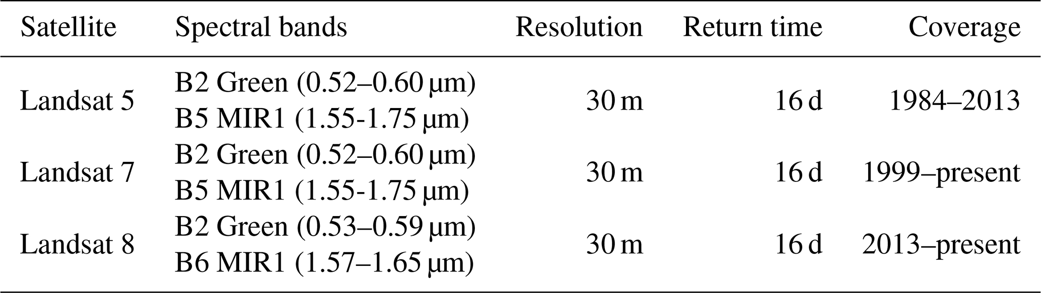
We focus on nine particular lakes – six gauged lakes in the US and three ungauged lakes outside the US (Fig. 2) – to illustrate the practical application of the gap-filling algorithm (Sect. 3.2) and discuss the validity of its four underlying assumptions in operational situations (Sect. 4). The six US lakes have between 17 and 47 years of daily water level observations, available from the United States Geological Survey and the Texas Water Development Board. The four water bodies in Texas are emblematic of changing seasonal to interannual lake conditions that prevail in intensively managed small lakes and reservoirs in semiarid areas. The two reservoirs in upstate New York represent the complex topography and strongly seasonal climate and land cover (including snow and ice) that prevail in high-latitude mountainous regions and complicate cloud and water detection. For each lake, monthly water extents were determined based on daily water levels, using the provided elevation–area–capacity tables and corrected for additive bias (see the Supplement). The three lakes outside the US have documented seasonal and interannual changes in their water extents that are of major regional significance, i.e., lakes Tonlé Sap (Cambodia), Urmia (Iran), and Chapala (Mexico). No long-term in situ observations were available for validation. However, we compared estimates from the Landsat 7 to estimates from Landsat 5 and 8 during respective overlapping periods. This process provides reasonable estimates of lake extent prediction errors, assuming that the sources of the errors across Landsat missions are close to independent (different sensors on different space platforms taking images at different times; see Table 1).

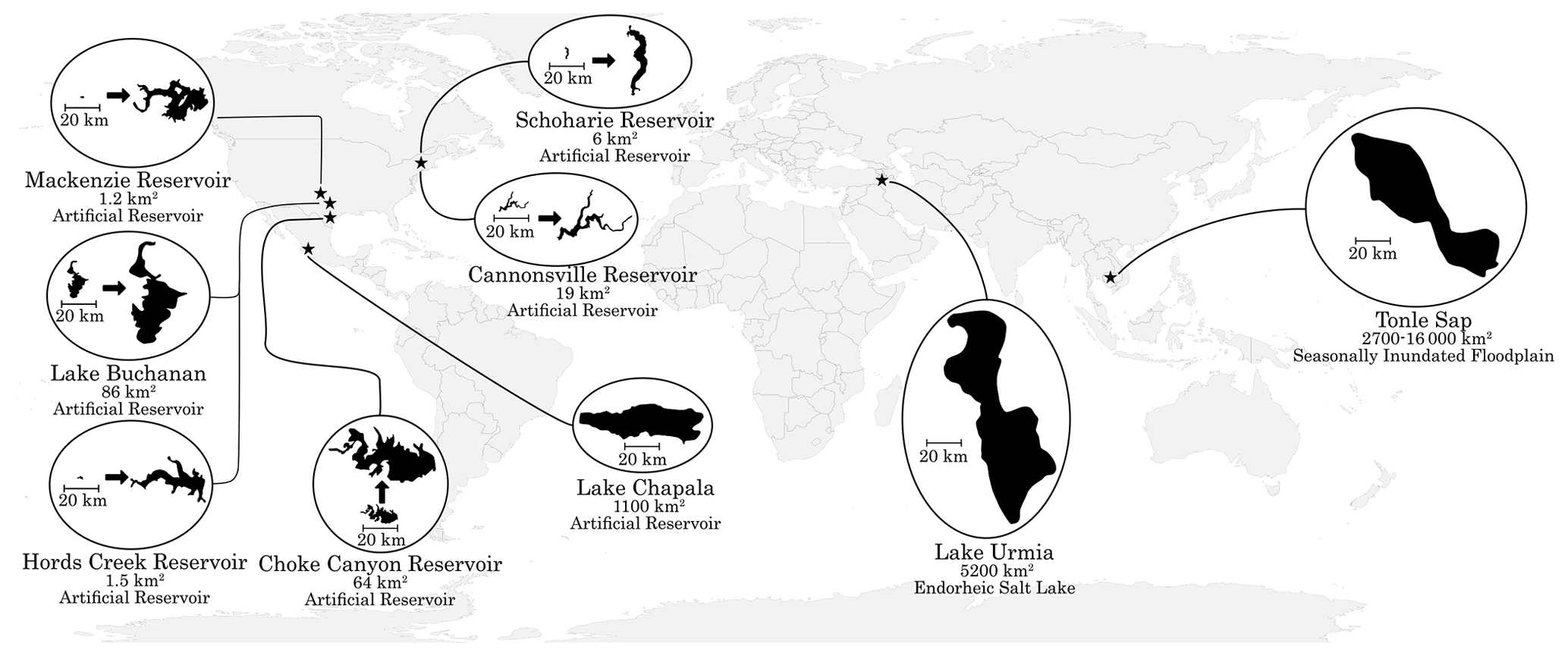
Figure 2 Location and characteristics of the considered water bodies.

Input to the gap-filling algorithm can be provided by any cloud- and water-detection method that is able to generate the required input ternary images. Here, we demonstrate its application using two particular techniques that are widely used in practice and straightforward to implement on Google Earth Engine, noting that more elaborate approaches to detect both clouds (Foga et al., 2017) and water (Rokni et al., 2014; Lu and Weng, 2007) on Landsat imagery are available. A rudimentary cloud-scoring algorithm, on the Google Earth Engine (ee.Algorithms.Landsat.simpleCloudScore()), is used to detect and mask clouds based on Top of Atmosphere Landsat reflectance images. Pixels indicated as faulty (e.g., due to the Landsat 7 Scan Line Corrector failure) are also masked out. The weekly to biweekly Landsat images are then aggregated at the monthly timescale through maximum value compositing using the Normalized Difference Vegetation Index (NDVI; Chen et al., 2003). This last step is based on the presumption that clouds have a low NDVI value. Cloud-free pixels of each monthly image were then classified as wet or dry, based on their modified normalized difference water index (MNDWI) value (Xu, 2006), i.e., the normalized difference between the green and mid-infrared bands of the relevant Landsat sensor (see Table 1 for corresponding bands in the considered imagery). The MNDWI enhances water/land contrasts by leveraging the ability of open water (compared to dry land) to preferentially absorb and reflect in the mid-infrared and green regions of the electromagnetic spectrum, respectively. A clustering algorithm is applied to each image to identify the MNDWI threshold that partitions its pixels into two sets so as to minimize the MNDWI variance within each set. Because it can dynamically separate dry and wet pixels in cloud-free images, unsupervised classification stands as a promising (and somewhat less arbitrary) alternative to the manual determination of classification thresholds implemented in past studies (e.g., Müller et al. (2016), among others). However, by minimizing within-cluster variance, k means tends to favor clusters of comparable sizes (Jain, 2010), which is problematic for cloudy images with preferential cloud covers on either land or water. As an extreme example, if all unmasked pixels are covered by water, a two-cluster k means classification will not be able to distinguish water from land. We address this issue by computing the median value from the set of MNDWI thresholds obtained from the classification of individual images. This single median MNDWI threshold is then used to (re)classify all unmasked pixels from all monthly images. Assuming the unsupervised classification can distinguish water from dry land on most images, the median threshold will allow for the identification of all unmasked pixels, from the above extreme example, as wet. A time series of lake area is finally generated by counting, on each monthly classified image, the number of inundated pixels within a predetermined polygon, encompassing the maximum historical extent of the lake. Outlier predictions associated with detection errors (see Sect. 4) are automatically identified and removed using the approach described in (Chen and Liu, 1993).

Table 1 Properties of Landsat data sources.

3 Results

3.1 Numerical validation

Results of the numerical experiments are presented in Fig. 3. Figure 3a displays gap-filling errors for various combinations of F₁ (pixels masked) and F₂ (pixels flipped). The former (F₁) represents the effect of the supervised classifier being provided with “too little” information in the sense that the cloud detector overestimates cloud coverage. Results in Fig. 3a suggest that this has a modest effect on gap-filling errors as long as the remaining (unmasked) pixels are correctly classified as water or land. Introducing even modest levels of classification errors in the unmasked pixels (e.g, F₂=5 %–10 % of unmasked pixels are flipped) can cause the gap-filling error to blow up for high levels of F₁. In other words, for sufficiently high cloud cover or small lake size, the accuracy of the approach becomes highly sensitive to classification errors, which occur in the example when more than 75 % of the lake is masked. Given that the lake in the synthetic analysis is ∼1 km², precautions should be taken when lakes are covered by excessive clouds or lakes are sufficiently small such that unmasked pixels cover less than 25 ha (or roughly 17×17 Landsat pixels).

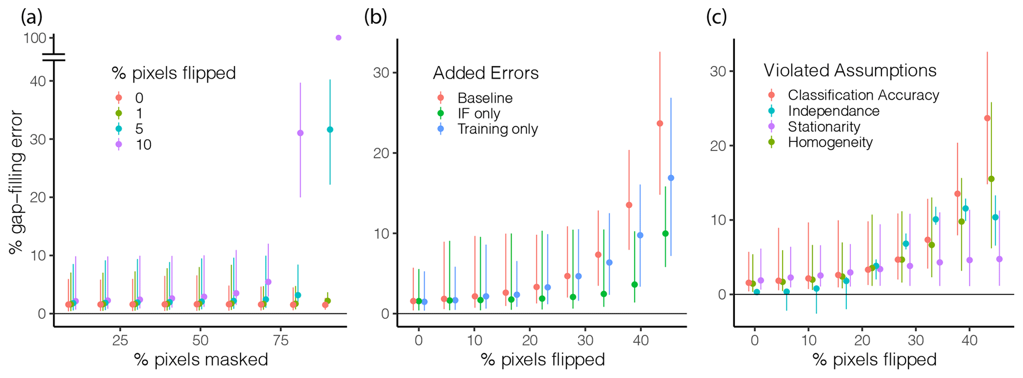
Figure 3 Results of the numerical experiments. (a) Gap-filling errors resulting from various combinations of independent random errors in cloud (percent of pixels masked) and water (percent of pixels flipped) detection. (b) Origin of the gap-filling errors associated with faulty land/water detection. Images with introduced errors are alternatively used to construct the IF raster (green) or the training data set (blue), or both inputs (red) of the supervised classifier are used to estimate the status of masked pixels. (c) Effect of deviations from the four fundamental assumptions obtained from the four numerical experiments described in Sect. 2.2. The percent of gap-filling errors in (b and c) were evaluated by masking 5 % of unmasked pixels in each image. These pixels were than used as validation data (step 1 in Sect. 2.2). Validation pixels were randomly and independently sampled for each image.

These classification errors are further investigated in Fig. 3b. Of note is that gap-filling errors arising from water–land classification errors (Fig. 3b) are generally larger than those arising from an overestimation of cloud cover (Fig. 3a). This suggests that the gap-filling approach works best when combined with an overly eager cloud-detection algorithm that tends to overestimate (rather than underestimate) cloud cover. Importantly, Fig. 3b also suggests that the gap-filling approach is generally robust to faulty water–land classification in input images. Introducing classification errors into up to F₂=30 % of unmasked pixels of each image causes gap-filling errors in less than 10 % of the control pixels. For context, a value of F₂=50 % would represent a situation in which wet and dry pixels are perfectly randomly distributed throughout the image (white noise). An F₂ value larger than 50 % reintroduces some signal; in particular, F₂=100 % has the same information as F₂=0 but with all wet and dry pixels being swapped. The numerical experiment also allows the assessment of the pathway through which input classification errors affect gap-filling performances. Specifically, the supervised classification is affected by (i) errors in the IF raster used as a predictor of inundation status for all images and by (ii) errors in the individual images used by the classifying as training. We investigate the relative importance of these two pathways by using the flipped images from step 2 (see Sect. 2.2) to either construct the IF raster or serve as training data for the classifier; unflipped images from step 1 are then used to fulfill the other task. Results in Fig. 3b suggests that the gap-filling algorithm is more sensitive to classification errors in its training data (blue) than to errors in its IF raster (green).

Results in Fig. 3c indicate the sensitivity of the gap-filling approach to deviations from each of its four underlying assumptions. The approach is most sensitive to errors in the detection of water and land in the input ternary imagery, although diversions from all four assumptions have a generally modest effect on gap-filling errors. As in Fig. 3b, gap-filling errors remain below 10 % for up to 30 % of pixels flipped (note that red symbols in Fig. 3b and c have an identical meaning). For higher levels of deviations (>30 % of pixels flipped), deviations from the independence (blue) and homogeneity (green) assumptions have comparable effects, which are both lower than that of classification errors (red) and higher than that of non-stationarities (purple). Note that the experiments used to evaluate stationarity and homogeneity assumptions are similar to the experiments for distinguishing the IF errors from training errors on Fig. 3b, with the important distinction that the errors introduced to evaluate the assumptions are persistent in space (i.e., they are not independently drawn for each input image). The negative values in the gap-filling errors obtained for the independence experiment (blue) arise from an image-by-image subtraction of classification errors that is included in the experiment (see Sect. 2.2). For particular images, the gap-filling error obtained from independently drawn classification errors is ostensibly larger than that obtained from persistent classification errors.

3.2 Application to real lakes

Applications to US lakes with available in situ lake level observations are presented in Figs. 4 (Hords, TX, Choke, TX, and Cannonsville, NY) and S1 in the Supplement (Buchanan, TX, Mackenzie, TX, and Schohaire, NY), where the gap-filling algorithm was combined with commonly implemented approaches to detect clouds and water on multispectral Landsat imagery. Lake area outputs from seven (brown) generally fit bias-corrected water extent estimates (black) are based on lake level observations, suggesting that the remote sensing approach was able to capture the strong temporal change in the water extent of these intensively managed reservoirs. Of note is that the outlier predictions, which were removed without user input (following Chen and Liu, 1993, and displayed as crosses in Figs. 4 and S2) predominantly concern lakes in upstate New York and are clustered in the winter season (shaded in Figs. 4 and S2). This points to known challenges in detecting open water in a landscape where land (and sometimes water) are covered by snow (e.g., Acharya et al., 2018). These challenges and their implications for the gap-filling algorithm are further discussed in Sect. 4. After removing winter classification results, lake extents estimated from Landsat 7 were strongly correlated to in situ observations for all lakes (Figs. 4 and S1).

Figure 4 Application to lakes with in situ observation data. (a, c, e) Time series representation water extent from the in situ observation (black) and Landsat 7 (brown). Automatically removed outliers (crosses) are also displayed for indicative purposes. Winter months (December to February) are shaded for Cannonsville, NY. (b, d, f) Scatterplot of absolute percentage errors on Landsat 7 water extent estimates (compared to in situ observations) against the proportion of the lake's maximum footprint that was covered by clouds.

Application to lakes Tonlé Sap, Urmia and Chapala, where no in situ observations are available, shows a high level of agreement across Landsat missions during overlapping periods (Fig. 5). The analysis suggests that recent fluctuations in the amplitude of the seasonal inundation cycles of Tonlé Sap, which are critical for maintaining its function as a regional biodiversity and food security hot spot, are decreasing. This is consistent with recent modeling simulations that predict decreased seasonal variations owing to flow regime alterations in the Mekong tributary region (Yu et al., 2019; Kummu and Sarkkula, 2008). The dramatic desiccation of Lake Urmia, once among the world's largest freshwater lakes, is also clearly visible in our analysis. Lake extent has declined steadily since the late 1990s, reaching a low point in August 2014, which is consistent with existing estimates (AghaKouchak et al., 2015). Similarly, large water fluctuations in Lake Chapala, a strategic and historically over-exploited reservoir in central Mexico (Wester, 2008; Godinez-Madrigal et al., 2019) in the 1990s and early 2000s, can be seen in our analysis, along with the effects of the dramatic (albeit controversial; Godinez-Madrigal et al., 2019) remediation policies that were implemented thereafter to restore lake levels (Wester, 2008).

Figure 5 Implementation of the approach on lakes with documented changes. (a, c, e) Time series of monthly lake extent estimates from Landsat 5 (blue), Landsat 7 (brown), and Landsat 8 (green) for lakes Urmia (a), Tonlé Sap (c), and Chapala (e). (b, d, f) Scatterplot of absolute percentage errors on Landsat 8 water extent estimates (compared to Landsat 7 estimates) against the proportion of the lake's maximum footprint that is covered by clouds.

4 Discussion

Results from the numerical experiments suggest that the performance of the gap-filling algorithm is generally robust to deviations from its four underlying assumptions. However, the analysis also showed that performance can be strongly impacted if these deviations are substantial enough. Therefore, the propensity of these four deviations to emerge in practice is an important question to consider when validating the proposed approach.

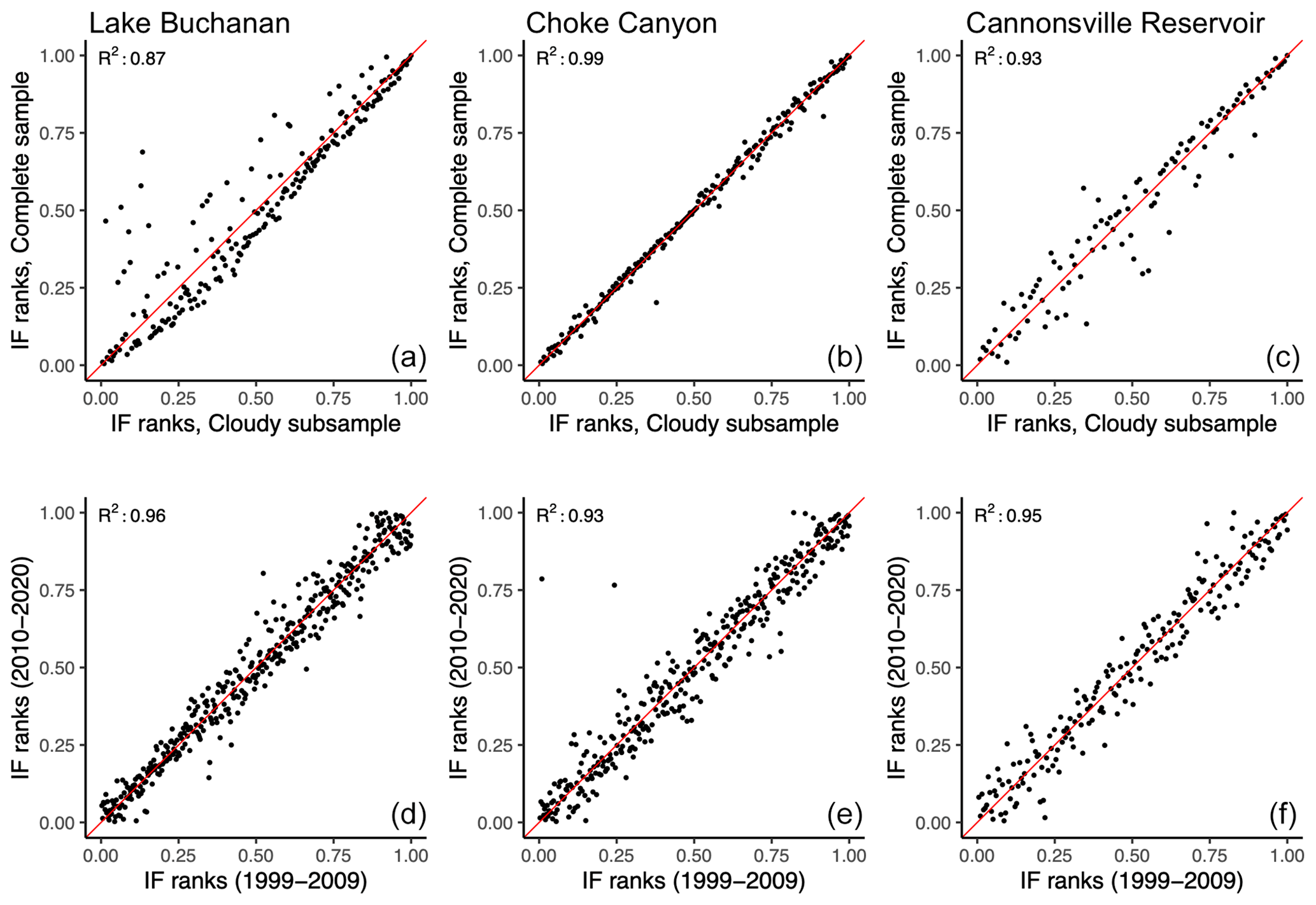
Figure 6 Assessment of the independence (a–c) and stationarity (d–f) assumptions for Lake Buchanan (a, d), Choke Canyon Reservoir (b, e), and Cannonsville Reservoir (c, f). (a–c) Inundation frequency ranks per pixel estimated under cloudless conditions (unsupervised classification; y axis) plotted against corresponding ranks estimated using the full sample of observations (combined supervised–unsupervised classification; x axis). (d–f) Inundation frequencies ranks per pixel estimated using the first (x axis) and second (y axis) half of the Landsat 7 observation period (1999–2019).

• Classification Accuracy. Despite its widespread use, the identification of clouds and water based on spectral indices entails inherent limitations. For example, challenges in distinguishing open water pixels from cloud or topographic shadows, or from snow-covered land, based on their MNDWI values, have been reported in the literature (see, e.g., Zhang et al., 2015; Huang et al., 2018b) and encountered in our analysis (Fig. 1e). However, the lack of direct in situ observations of lake extents and the highly local nature of the error source (e.g., topography, snow cover) make it challenging to estimate their general prevalence. Instead, we find it helpful to characterize classification errors as having two distinct and alternative effects. On the one hand, misclassification of either land or water as clouds, for instance due to an overly eager cloud detector, will decrease the amount of input information (too little information). On the other hand, misclassification of water (or land) as land (or water) will introduce an error into the input information (wrong information). This situation can emerge from an overly cautious cloud detector, where undetected clouds are then arbitrarily classified as either water or land. Results from the numerical experiments suggest that wrong input information has a much larger effect on the gap-filling performance than too little input information (compare red symbols in Fig. 3a and b). This insight is corroborated by comparing two sets of lakes from the case studies. The approach performed well for the two small lakes in Texas (Hords Creek and Mackenzie Reservoir; ∼1 km² each), where the semiarid climate and the flat topography are not prone to water classification error, but their small size limits the number of input pixels (too little information). In contrast, the two lakes in upstate New York (Schoharie and Cannonsville reservoirs) have more input pixels, but the cold climate and mountainous terrain introduce errors in the unsupervised classification of water and land (wrong information). There, the gap-filling algorithm performed markedly worse, particularly in winter when snow and ice are prevalent. These results illustrate a key limitation of the approach, i.e., that gap-filling accuracy is constrained by the accuracy of the input ternary imagery. They also suggest that the approach is more compatible with an overly eager cloud detector. By overestimating cloud cover, the input imagery will err in favor of providing too little (rather than wrong) information, which has a smaller effect on the accuracy of the gap-filling algorithm. The benefits of an over-eager cloud-detection algorithm will be limited when unmasked pixels cover a sufficiently small area (roughly 20–30 ha), at which point accuracy becomes highly sensitive to wrong information.

• Independence. A threat to the independence requirement may emerge if the inundation status of a pixel determines its cloud coverage. For instance, fog can be produced by the micro-climatic conditions associated with open water (Koračin et al., 2014). We test whether threats to the independence assumptions emerged in our case studies by comparing the inundation frequency of pixels during cloudless days with their inundation frequency estimated for all days. The former corresponds to the IF value from Eq. (1). The latter was determined by computing the estimated IF values of pixels after gap filling, which includes cloudy days. We sampled 4000 pixels with IF values between (and excluding) 0 and 1 for both images (before and after gap filling). We then ranked the pixels according to their IF value for each image. The independence assumption implies that the pixel rank is not affected by its cloud coverage status. A pixel with a higher inundation frequency than another for a subset of observations that had cloudless conditions should also have a higher inundation frequency if the full sample of observations (cloudless and cloudy) is considered. Results, shown in Fig. 6a–c, suggest that the ranking of inundation frequency does not depend on cloud coverage. In other words, the independence assumption does not appear to be threatened in the considered lake. Note that non-random cloud coverage will only affect classification output if it concerns pixels near shores (i.e., where $\mathrm{0}<\text{IF}<\mathrm{1}$). This excludes permanently inundated pixels, which are predominantly affected by fog over water (Koračin et al., 2014).

• Stationarity. We used a split-sample approach to determine whether the relationship between IF and the inundation status of pixels remains constant over time. A total of two IF images were constructed using the first (1998–2009) and second (2010–2020) half of the available Landsat 7 images. The inundation frequencies given by the first and second IF images were then collected for a random sample of 5000 pixels, with $\text{IF}\in [\mathrm{0},\mathrm{1}]$ in both images. The sampled pixels were then ranked according to their IF value for each image. The stationary assumption implies that the rank of the pixels does not vary between the two observation periods. If the bathymetry did not change, a pixel that is more often inundated than another pixel during the 1998–2009 period should still be inundated more often during the 2010–2020 period. Results in Fig. 6 (bottom) suggest that the effect of bathymetric change on the classification outcome is negligible. Note that classification outcomes are only affected by bathymetric changes that concern those pixels that lie within the range in the variability of the water extent. This excludes pixels that are permanently covered (IF=1), where bathymetry may be most affected by sedimentation processes.

• Homogeneity. The homogeneity assumption implies that the relationship between the historical inundation frequency of a pixel and its current inundation status does not vary in space. In other words, pixels that are historically more often inundated will more likely be inundated on any given day. This assumption clearly holds for the non-disjoint bodies of water that are considered in this study but may not apply to bodies of water that fragment upon drainage (Fig. 7). There, the gap-filling algorithm should be applied independently for each homogeneous region. The need to identify homogeneous regions a priori in fragmenting lakes and more complex wetland landscapes is an important limitation of the approach.

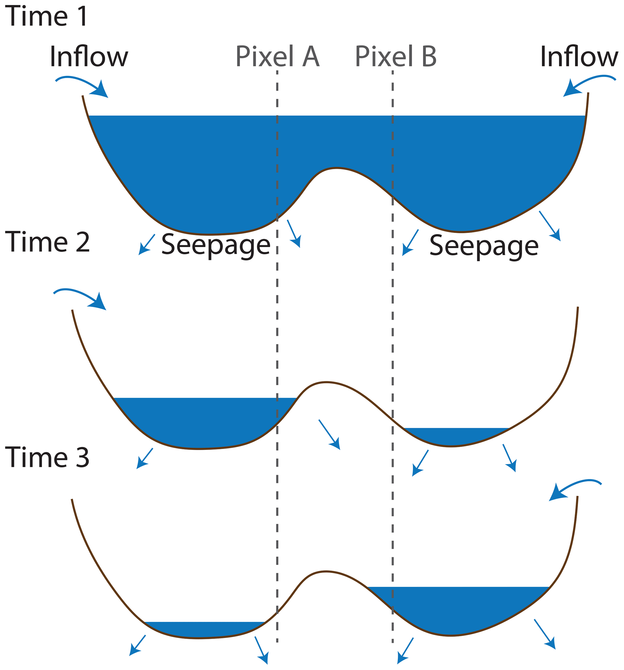
Figure 7 Violation of the homogeneity assumption in a fragmenting lake. A single body of water (top) might fragment into independent fragments when draining (middle and bottom). In the figure, the lake is drained by seepage, and the two fragments are supplied by distinct tributaries. Under these conditions, pixels A and B might have an identical IF value but do not have an identical flooding status at times 2 and 3 and, hence, violate the homogeneity assumption.

5 Conclusion

We propose a gap-filling approach that uses a standard supervised classification algorithm to predict the binary status (wet–dry) of masked pixels based on the historic frequency of their status. We validate the approach by (i) using numerical simulation to assess its sensitivity to deviations from its four fundamental assumptions and (ii) applying it to nine global lakes representing a variety of sizes, climates, topographies, and levels of in situ data availability. Applying the approach to real lakes also allows us to evaluate the propensity for fundamental assumptions of the approach to hold in practical situations. Both analyses suggest that the approach is robust to substantial deviations from its underlying assumptions, several of which are likely to hold in most practical settings. However, the analyses also outlined two important limitations of the approach. First, the approach is sensitive to classification errors in the input imagery, particularly in small lakes. Misclassification of the output binary classes (here wet/dry) have a stronger impact on performance than the misidentification of masked pixels (here clouds), and the effect is exacerbated when unmasked lakes pixels fall below 25 ha (roughly 17×17 Landsat pixels). This further implies that the approach might not perform well in locations in which circumstances (topographic shading, cloud shading, snow/ice, etc.) make it difficult to reliably distinguish water from clouds and land using multispectral imagery. In contrast, the method appears generally robust to situations where a limited number of input classified pixels are available for training (e.g., small lakes or high cloud coverage). These two observations imply that the approach is preferably combined with a cloud detector that tends to overestimate cloud coverage. Second, the approach requires the a priori identification of homogeneous regions, where the relationship between the inundation frequency and inundation status of pixels is unique. This requirement limits the scalability of the approach in complex wetland landscapes, where the relationship might vary through space.

Despite these limitations, the approach stands as a promising approach (it can be readily implemented in Google Earth Engine; see the code and data availability section) to monitor the water extent of lakes and reservoirs at scale, particularly when combined with recent global data sets of ternary (wet, dry, or masked) water cover (Pekel et al., 2016a; Donchyts et al., 2016). More generally, the algorithm can be used to infer the status of any masked binary imagery (not only water cover) that satisfies its four fundamental assumptions.