Multivariable evaluation of land surface processes in forced and coupled modes reveals new error sources to the simulated water cycle in the IPSL (Institute Pierre Simon Laplace) climate model

Evaluating land surface models (LSMs) using available observations is important for understanding the potential and limitations of current Earth system models in simulating water- and carbon-related variables. To reveal the error sources of a LSM, five essential climate variables have been evaluated in this paper (i.e., surface soil moisture, evapotranspiration, leaf area index, surface albedo, and precipitation) via simulations with the IPSL (Institute Pierre Simon Laplace) LSM ORCHIDEE (Organizing Carbon and Hydrology in Dynamic Ecosystems) model, particularly focusing on the difference between (i) forced simulations with atmospheric forcing data (WATCH Forcing Data ERA-Interim – WFDEI) and (ii) coupled simulations with the IPSL atmospheric general circulation model. Results from statistical evaluation, using satellite- and ground-based reference data, show that ORCHIDEE is well equipped to represent spatiotemporal patterns of all variables in general. However, further analysis against various landscape and meteorological factors (e.g., plant functional type, slope, precipitation, and irrigation) suggests potential uncertainty relating to freezing and/or snowmelt, temperate plant phenology, irrigation, and contrasted responses between forced and coupled mode simulations. The biases in the simulated variables are amplified in the coupled mode via surface–atmosphere interactions, indicating a strong link between irrigation–precipitation and a relatively complex link between precipitation–evapotranspiration that reflects the hydrometeorological regime of the region (energy limited or water limited) and snow albedo feedback in mountainous and boreal regions. The different results between forced and coupled modes imply the importance of model evaluation under both modes to isolate potential sources of uncertainty in the model.

1 Introduction

Land surface models (LSMs) are essential for understanding the large-scale exchange of energy, water, and carbon between the land surface and the atmosphere. LSMs coupled with atmospheric general circulation models (GCMs) have been used to simulate global climate and climate change under international frameworks, such as the Coupled Model Intercomparison Project (CMIP; Taylor et al., 2012; Eyring et al., 2016a), contributing to Earth sciences and policymaking for mitigating and adapting to climate change. To understand the potential and limitations of climate change simulations, evaluating outputs of LSMs with available observations is important (Flato et al., 2013). Uncertainties associated with LSMs can arise from a deficiency in model physics and parameterization (Liu et al., 2003), errors in atmospheric forcing data (Guo et al., 2006; Nasonova et al., 2011; Yin et al., 2018), boundary conditions, including vegetation and land use changes (Guimberteau et al., 2017; Boisier et al., 2014), and/or error propagation through land–atmosphere coupling (so-called “climate drift”; Dirmeyer, 2001). Recently, convenient tools for systematic model evaluation have been developed (e.g., Eyring et al., 2016c; Gleckler et al., 2016; Best et al., 2015); however, further in-depth model evaluation is required to reveal the underlying processes and sources that lead to uncertainties in simulations (Eyring et al., 2016b).

Notably, focusing on the differences between LSM simulations with and without GCM coupling would provide novel knowledge about LSM evaluation (Liu et al., 2003; Zabel et al., 2012; T. Wang et al., 2015). LSM simulations that are without GCM coupling but are forced by an atmospheric data set (also called “offline” or “stand-alone” mode) do not allow feedback between the atmosphere and land surface. Therefore, errors in the simulated values solely arise from deficiency model structure/parameterization, uncertainty in the forcing data (Yin et al., 2018), and mismatch in land cover between model and forcing data (Zabel et al., 2012). The foremost influential forcing factor on the water cycle is precipitation (Qian et al., 2006; Decharme and Douville 2006), although radiation and land cover (i.e., vegetation) can also affect hydrological variables (Dirmeyer, 2001; Guo et al., 2006) such as surface soil moisture (SSM) or evapotranspiration (ET), depending on the temporal scale (Guo et al., 2006) and the hydrometeorological condition of the region (i.e., energy limited or water limited; Nasonova et al., 2011; Zabel et al., 2012). Anthropogenic factors (e.g., irrigation) may also cause errors in the simulated variables when not accounted for by the LSM (Yin et al., 2018). On the other hand, coupled LSM simulations are also affected by errors in atmospheric simulation, which can be enhanced through land–atmosphere interaction (Mahfouf et al., 1995; Liu et al., 2003; T. Wang et al., 2015). Such errors occur at short timescales (i.e., several days) up to seasonal timescales (Dirmeyer, 2001) via the interlinkage of hydrological variables (e.g., rainfall, SSM, ET, and infiltration) in the LSM scheme and thermal variables (Cheruy et al., 2017; Ait-Mesbah et al., 2015).

Among the various LSMs, we focused on the Organizing Carbon and Hydrology in Dynamic Ecosystems (ORCHIDEE) LSM (e.g., Krinner et al., 2005; d'Orgeval et al., 2008; Guimberteau et al., 2017), which enables the explicit representation of processes governing the water, carbon, and energy budgets with a highly flexible spatial resolution (Raoult et al., 2019). We used the ORCHIDEE (revision 4783; tag 2.0) version, which is implemented in the IPSL's (Institute Pierre Simon Laplace) climate model (CM) configurations used for CMIP6 (Eyring et al., 2016a), including the Land Surface, Snow and Soil Moisture Model Intercomparison Project (LS3MIP), with offline simulations (van den Hurk et al., 2016). Through an in-depth assessment of five simulated variables (i.e., SSM, ET, leaf area index (LAI), surface albedo, and precipitation) that should be closely interlinked, and a special focus on the differences between forced and coupled simulations, the aim of this study is to better understand which land surface processes deserve further improvements in the studied LSM and to investigate the land–atmosphere coupling role in diagnosed model uncertainties.

The Global Climate Observing System (GCOS, 2010) designates the five selected variables as being essential climate variables (ECVs), thereby allowing us to take advantage of recent progress in their global-scale observation. Using satellite data, researchers have developed various retrieval algorithms to acquire SSM (Jackson et al., 1999; Wigneron et al., 2007, 2017), ET (Zhang et al., 2010; Miralles et al., 2011; Zeng et al., 2014), LAI (Zhu et al., 2013), albedo (Schaaf et al., 2002; Qu et al., 2014), and precipitation (Adler et al., 2003) which can be used as reference data for LSM evaluation. Empirical upscaling products from global in situ observations (Jung et al., 2011, 2019) can also be used. The selected variables are particularly interesting for land surface processes; SSM is a recognized driver of surface–atmosphere interactions (Seneviratne et al., 2010), constraining the partitioning of sensible/latent heat and plant activity and determining ET and vegetation dynamics (e.g., Gu et al., 2006). ET affects atmospheric humidity (usually described by the vapor pressure deficit) and cloud formation, creating feedback systems among SSM, ET, and precipitation (Yang et al., 2018). Accounting for long-term vegetation dynamics, which can be measured by LAI, interlinked with such hydrological processes, is important in monitoring carbon cycle and ecosystem services that are related to climate change (IPCC, 2014) and natural disasters (Adikari and Noro, 2010). Another important parameter in the surface energy exchange is the surface albedo, which controls the reflection of incident solar radiation and is interlinked with hydrological processes (especially through surface snow cover) and vegetation dynamics (Bonan, 2008).

To investigate the potential sources of model uncertainty, we considered various landscape factors (“factor analysis”) in addition to the traditional statistical evaluation. This work aims at increasing knowledge about the features and limitations of ORCHIDEE and is a practical example of in-depth model evaluation focusing on the differences between forced and coupled modes. The remainder of this paper is organized as follows. Section 2 describes the simulation setting, the reference data sets, and the factor analysis. Section 3 presents results for the spatiotemporal patterns of the model uncertainties and factor analysis. Finally, Sects. 4 and 5 provide a discussion and conclusions, respectively.

2 Materials and methods

2.1 Model and simulations

2.1.1 Description of the land surface model

ORCHIDEE (Organizing Carbon and Hydrology in Dynamic Ecosystems) is the LSM used in the IPSL Earth System Model (ESM). This global process-based model of the land surface describes the complex links between the terrestrial biosphere and the water and the energy and carbon exchanges between the land surface and the atmosphere (Krinner et al., 2005). The used version in the IPSL-CM6 ESM for the CMIP6 simulations (Boucher et al., 2020), which is known as tag 2.0, was previously described in many papers (Raoult et al., 2019; Boucher et al., 2020; Cheruy et al., 2020; Tafasca et al., 2020), and we only summarize its main features in this paper, with some details on the related parameterizations to the five studied ECVs.

The land cover is described with 15 plant functional types (PFTs), including one for bare soil, as seen in the full list in Table 2, and they can all coexist in each grid cell, where the fractions used here are from the CMIP6 data sets (Boucher et al., 2020). For each PFT, the transpiration serves as a coupling flux between the water, energy budget, and photosynthesis process, which drive the evolution of the biomass and LAI owing to generic equations with PFT-specific parameters (Krinner et al., 2005). Evapotranspiration (ET) is controlled by the energy and water budget via a bulk aerodynamic approach, where the following four parallel fluxes are distinguished: sublimation, interception loss, soil evaporation, and transpiration. In each grid cell, the first two fluxes proceed at a potential rate from the grid cell fractions with snow and canopy water, respectively. The soil evaporation and transpiration originate from the complementary snow-free fractions covered by bare soil and vegetation which depend on LAI, as the effectively foliage-covered fraction exponentially increases with LAI. These two fluxes depend on soil moisture; transpiration is limited by the stomatal resistance, which increases when soil moisture drops from field capacity to wilting point; soil evaporation is not limited by a resistance but only by upward capillary fluxes, which control the soil propensity to meet the evaporation demand.

The soil moisture (SM) dynamics are described over a soil depth of 2 m and discretized into 11 soil layers to solve the Richards equation. SM in the top 10 cm is regarded as SSM. The hydraulic conductivity and retention properties depend on the SM owing to the van Genuchten–Mulaem equations, with parameters depending on the soil texture (Tafasca et al., 2020), which is read from the map of Zobler (1986). The infiltration is limited by the surface hydraulic conductivity, and it is calculated with a time-splitting procedure inspired by the Green–Ampt equation, where a sharp piston-like wetting front is assumed (d'Orgeval et al., 2008; Vereecken et al., 2019). The surface runoff is made of non-infiltrated water (infiltration-excess runoff); however, ponding is allowed in flat areas, and it can reinfiltrate at later time steps. This so-called reinfiltration fraction linearly decreases from 1, in totally flat grid cells, to 0, where the mean grid cell slope exceeds 0.5 %. For CMIP6, the ORCHIDEE model does not include the irrigation impact on the SM, ET, and vegetation growth, although the model can simulate this anthropogenic pressure (Xi et al., 2018).

The snow processes are described by a three-layer scheme of intermediate complexity (Wang et al., 2013) in which the snow albedo and insulating properties depend on the snow density and age. The ORCHIDEE 2.0 also includes a revised parameterization of the interplay between the vegetation and the snow albedo, and the optimized parameters match the remote sensing albedo data from the Moderate Resolution Imaging Spectroradiometer (MODIS) sensor, distinguishing the visible and near-infrared (NIR) bands (Boucher et al., 2020). For the calculation of the heat diffusion, which includes the soil-freezing effects (permafrost), the soil is extended to 90 m, and the moisture content of the deepest hydrological layer is extrapolated to the entire profile between 2 and 90 m. The thermal soil properties depend on the soil texture, moisture, and carbon content (Guimberteau et al., 2018).

2.1.2 Forced and coupled simulations

To separate the errors caused by the ORCHIDEE model structure/parameterization from the ones resulting from the simulated climate through land–atmosphere coupling, we compared a forced and a coupled simulation. In the coupled simulation, the ORCHIDEE LSM is coupled to the LMDZ6A atmospheric GCM (Hourdin et al., 2020), as embedded in the IPSL-CM6 ESM for the CMIP6 simulations (Boucher et al., 2020; Cheruy et al., 2020). The only difference between the atmospheric physics used in this paper and the one used for CMIP6 concerns the parameterization of deep and shallow convection and their interaction, modified to improve the description of the intertropical convergence zone and the El Niño–Southern Oscillation. The description of these differences and their impact on precipitation and other variables controlling the near-surface climate can be found in Mignot et al. (2021).

The coupled simulation was run over 1985–2014 (following a 5-year spin up), using a “nudging” approach to constrain the large-scale atmosphere dynamics toward the synoptic atmospheric conditions (Cheruy et al., 2013). To this end, the simulated wind fields (zonal and meridional wind components) are relaxed toward the ERA-Interim winds (Dee et al., 2011) by adding a correction term in the evolution equation for the wind. By reducing the internal variability, this method allows the direct comparison of the observations and simulations, and it was successfully used for evaluating the coupled land–atmosphere parameterizations (Cheruy et al., 2013; Wang et al., 2016), including with the IPSL-CM6 ESM (Cheruy et al., 2020).

In the forced simulation, which covers 1979–2009, the required near-surface meteorological data by the ORCHIDEE LSM (liquid and solid precipitation, incoming longwave and shortwave radiation, 2 m air temperature and specific humidity, 10 m wind speed, and surface pressure) are prescribed from the downscaled and bias-corrected reanalysis data (WATCH Forcing Data ERA-Interim – WFDEI), provided at the 0.5^∘ resolution with a 3 h time step (Weedon et al., 2011, 2014). Precipitation is bias-corrected using monthly data from the Global Precipitation Climatology Centre (GPCC version V6; Schneider et al., 2014), with a specific correction of undercatch errors, following Adam and Lettenmaier (2003).

The spatial resolution differs between the two simulations, reflecting the grid of the atmospheric data; the coupled simulation has a coarser resolution (144 × 142, corresponding roughly to 2.5^∘ in longitude and 1.25^∘ in latitude) than that of the forced simulation (0.5^∘ grid). To make the evaluation consistent and simple, we used the same spatial resolution for our analyses, and we oversampled the LMDZ6A grid mesh to the finer resolution (0.5^∘) so as to keep as much spatial information as possible from the high-resolution offline grid mesh. To investigate variability patterns on seasonal to interannual scales, all the data were aggregated into monthly time steps. A total of five interlinked variables (SSM, ET, LAI, albedo, and precipitation) were considered in this evaluation, and the study region was 60^∘ S–90^∘ N, 180^∘ W–180^∘ E (i.e., Antarctica and Greenland were excluded).

2.2 Reference data

2.2.1 Surface soil moisture

The SSM product provided by European Space Agency Climate Change Initiative (ESA CCI; Liu et al., 2012) was used as a reference. It is a merged product comprising multiple SSM data derived from various passive and active microwave satellites (i.e., SMMR, SSM/I, TMI, AMSR-E, Windsat, SMOS, AMSR2, AMI-WS, ASCAT-A, and ASCAT-B) providing a long-term (1978–2018) SSM data set with 0.25^∘ resolution. The CCI-SSM product has been evaluated extensively against in situ observations (e.g., Al-Yaari et al., 2019b), and their accuracy has been reported as being relatively high compared to that of other existing products such as SMOS-L3, LPRM, and AMSR2 (Ma et al., 2019).

Because it includes low-quality data flags for snow, dense vegetation, and radio frequency interference (RFI; Oliva et al., 2012), we applied data screening following Al-Yaari et al. (2016). We screened out all the pixels where the provided uncertainty was larger than 0.06 m³/m³ (volumetric water content). Next, any data records in which the SSM was not in a valid range (either >0.6 or <0.0; Fernandez-Moran et al., 2017; Dorigo et al., 2013) were excluded. Finally, to exclude any areas covered by snow or dense vegetation and other unreliable regions, we kept only those areas in which the quality flag was zero (fine quality pixels). The screened data set was then aggregated into 0.5^∘ × 0.5^∘ and monthly time steps. This screening process removed 3.6 % of all the original pixels.

We performed an initial check on the time series of the global average of CCI-SSM and found an artificial trend therein that depended on the availability of the observation data (Fig. S6 in the Supplement). As reported by other researchers (e.g., Loew et al., 2013), this artificial trend could lead to misinterpretation of long-term signals. To mitigate such artificial trends and initialization errors of each data, we selected a stable period (i.e., without a discontinuous jump in time series) during 1993–1999 for comparison with both the forced and coupled simulations. Because of the differing natures of LSM-simulated and LSM observed SSM (e.g., dependence on meteorological forcing data/atmospheric model and model parameterization), their absolute SSM (m³/m³) values (i.e., magnitudes) are not comparable (Reichle et al., 2004). In addition, since the CCI-SSM product is scaled by the comparison with a different LSM (GLDAS-Noah), a direct comparison between CCI-SSM and ORCHIDEE may lead to misleading results, as they have different soil representation (Raoult et al., 2019). Given this issue, the LSM- and satellite-based SSM were compared with statistically normalized values rather than absolute values of SSM (e.g., Polcher et al., 2016). Therefore, a spatiotemporal normalization (Eq. 1) was applied to each co-masked data set to eliminate systematic biases among the data sets and make the comparison reliable (Fig. S7B) as follows:

$$\begin{array}{}\text{(1)}& {\mathrm{SSM}}_{\mathrm{norm}}={\displaystyle \frac{\mathrm{SSM}-\stackrel{\mathrm{‾}}{\mathrm{SSM}}}{{\mathit{\sigma }}_{\mathrm{SSM}}}},\end{array}$$

where SSM_norm is the normalized SSM, and $\stackrel{\mathrm{‾}}{\mathrm{SSM}}$ and σ_SSM are the mean and standard deviation, respectively, of all the available SSM sampled along spatial and temporal dimension during the period.

2.2.2 ET

In a preliminary study, we compared a ground-based machine learning ET product (Jung et al., 2011, 2019), three remote-sensing-based physical model products (Miralles et al., 2011; Zhang et al., 2010; Zeng et al., 2014), and their ensemble (see Figs. S2 and S7). We found that they showed similar spatiotemporal structures although they differed in absolute values in some regions, and the ground-based product was the most consistent with the ensemble. Therefore, we decided to use the ground-based ET (millimeters per day) as a representative from 1987 to 2009. It is also advantageous in that it is derived from the upscaling of FLUXNET data (Jung et al., 2011, 2019) and is independent from specific ET retrieval algorithms. The original spatial resolution (1^∘) of the data was resampled into 0.5^∘ resolution to match that of the forced simulation, and the original temporal resolution was monthly time steps. A preliminary check of the time series and spatial patterns of the reference data revealed no artifact patterns (e.g., no abrupt jump in time series as found in CCI-SSM), so we used them with no pixel screening or normalization.

2.2.3 LAI

We used the global LAI data set of Zhu et al. (2013), referred to hereinafter as LAI3g, which is based on a neural network algorithm in conjunction with the third-generation Global Inventory Modeling and Mapping Studies (GIMMS 3g) and MODIS LAI product, with an original spatial resolution of 0.5^∘ and a half-monthly temporal resolution. Considering the common period among LAI3g and the coupled and forced simulations, we selected 1987–2009 as the comparison period, and we resampled all data at 0.5^∘ spatial resolution and aggregated them into monthly time steps.

2.2.4 Albedo

We used the MODIS albedo product (Qu et al., 2014) as reference data, which provided the bi-hemispherical reflectance (white sky albedo) for the visible and NIR bands. The original 500 m spatial resolution and 16 d temporal resolution were resampled (i.e., upscaled) into 0.5^∘ resolution and monthly time steps. The common period between simulations and observation, 2003–2009, was used for evaluation. The pixels with a retrieval failure of the albedo were excluded from the analysis.

2.2.5 Precipitation

We also evaluated the simulated precipitation because it is the primary factor that influences the hydrological variables (Qian et al., 2006; Decharme and Douville, 2006). To this end, we used the GPCC data set version 6 (Schneider et al., 2014), which was also used to bias correct the WFDEI meteorological forcing of the offline ORCHIDEE simulation (Sect. 2.1.2). This gridded product at 0.5^∘ provides monthly precipitation, derived from quality-controlled observed precipitation from over 65 000 stations worldwide, and accounts for a climatological correction of undercatch based on Legates and Willmott (1990).

2.2.6 Data processing

For consistency between the observed and simulated data, we subjected the former to aggregation or resampling toward the 0.5^∘ spatial resolution and monthly time steps for each variable, as described above. Due to the presence of data gaps in the reference data sets, which are either because of the acquisition issues or the quality control and data screening, we masked the simulated data sets to match the spatiotemporal data availability of the corresponding reference data. For the SSM, the dense snow regions (with a snow water equivalent exceeding 48 mm) in the simulated data were further excluded so as to avoid unreliable comparisons with uncertain references. Also, co-masking was performed after the spatiotemporal resampling, followed by the statistical normalization (only for the SSM). The resulting coverage of the selected comparison period is summarized in Table 1 for each variable.

Table 1 Overview of the selected reference data sets and period of analysis. The last column gives the percent of land pixels, in the maps of Figs. 2 and 3, with observed values. A smaller amount of SSM data is available compared to the others as a result of relatively strict quality control. For ET and LAI, no data were available in extremely arid regions.

After the abovementioned preprocessing, to compare the spatial patterns of the observed and simulated data, we focus on the following three accuracy criteria calculated at the 0.5^∘ scale along monthly time steps: the bias, Pearson's correlation coefficient (CC), and root mean square error (RMSE). The criteria were calculated along the temporal axis for each pixel (i.e., the result was shown as one global map for a criterion). The statistical significance of the bias (compared to zero) and CC was assessed at each pixel with Student's t test and Pearson's test, respectively, with a p value of 5 % in both cases. Note that the evaluation periods were different among SSM (1993–1999), ET, LAI and precipitation (1987–2009), and albedo (2003–2009). However, the impact of the chosen period on the evaluation is likely to be limited (see Table S1 in the Supplement).

2.3 Factor analysis

To reveal features of the simulations in detail, the accuracy criteria were evaluated against various landscape/meteorological factors (Fig. 1), namely PFT, LAI, irrigation, precipitation, slope, snow, and ET. For each factor, time series were averaged temporally to make only one global map (i.e., the classification criteria were applied on long-term basis). The value of each factor was classified into a specific number of levels (classes), which were used as ordinal scales. Each factor was classified as given in Table 2, and each factor is described in detail below:

1. For PFT, we used the input data set that is used in ORCHIDEE. This includes fractional coverages in each pixel of 15 PFTs. We created a dominant PFT map by picking up the PFT class that has maximum fractional coverage for each pixel.

2. For LAI, we used the LAI3g data (Sect. 2.2.3), classifying them into three levels (see Table 1 for the specific class definitions).

3. For irrigation, we used a global map of irrigation areas (Siebert et al., 2010), which indicates the fractional coverage (%) of an irrigated area with 5 arcmin spatial resolution. It was classified into six levels.

4. For precipitation, we used the pluriannual mean of GPCC during the same period as the investigated ECVs. It was classified into five levels.

5. For slope, this classification was done by referring to the ETOPO5 DEM (5 arcmin global relief model of Earth's surface; NOAA, 1988), which is also used in ORCHIDEE to control reinfiltration of the water.

6. We used the pluriannual mean of the forced SWE for the factor analysis of the forced simulation and that of the coupled SWE for the coupled simulation. The SWE was classified into five levels.

7. For ET, we used the pluriannual mean of Jung et al. (2011, 2019) during the same period as the investigated ECVs.

Here, the dominant PFTs, irrigation, slope, and SWE were only used for the factor analysis, while LAI, precipitation, and ET were also used for validation and come from independent sources. The PFT fractions and SWE, however, were not independent from our simulations, but we assumed it was not problematic for factor analysis, which mostly aims at suggesting process-based explanations to the main model errors.

Table 2 Correspondence between classification levels and values for each factor.

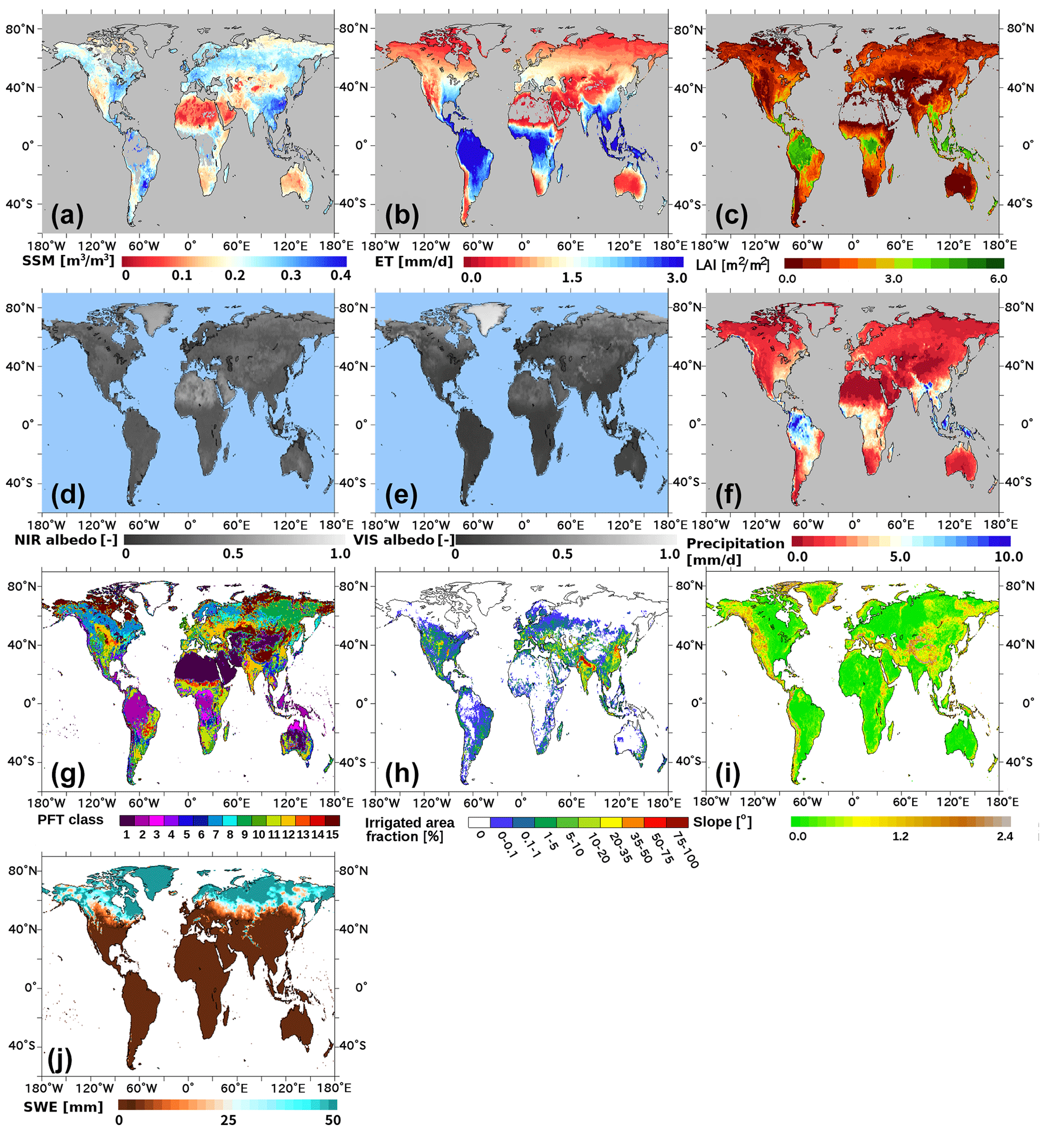
Figure 1 Spatial patterns of pluriannual mean reference data used for validation (marked with +) and/or factor analysis (marked with ×). (a +) SSM from ESA CCI. (b $+\times$) ET product of Jung et al. (2019). (c $+\times$) LAI3g. (d +) MODIS NIR albedo. (e +) MODIS visible albedo. (f $+\times$) GPCC precipitation data. (g ×) Dominant plant functional type used in ORCHIDEE (see Table 2 for the class definition). (h ×) Fractional area equipped with irrigation. (i ×) Slope derived from ETOPO5. (j ×) Snow water equivalent derived from the forced-mode ORCHIDEE.

3 Results

3.1 Spatial and temporal patterns of model errors

Overall, the spatial structures of the ECVs simulated in both modes were consistent with those of the reference products, as shown by comparing the corresponding pluriannual mean maps (Figs. S1–S5). To refine this comparison, Fig. 2 shows the spatial bias patterns of the five variables (normalized SSM, ET, LAI, albedo, and precipitation), in both forced and coupled modes. Differences between forced and coupled modes are also shown in Fig. S6. Spatiotemporal averages of bias, RMSE, and correlation coefficients are summarized in Table 3. The spatial patterns of the temporal CC are also shown for SSM and albedo (Fig. 3) for further discussion.

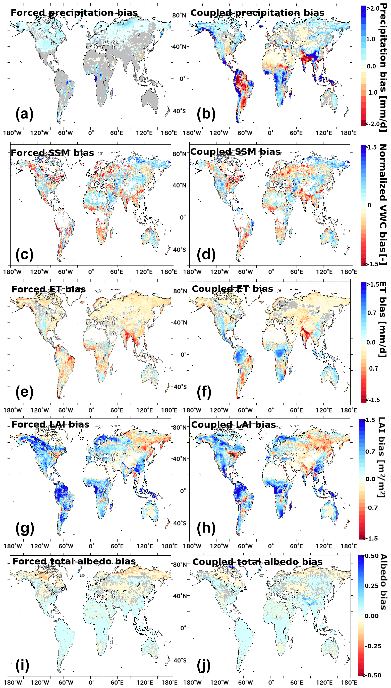
Figure 2 Pluriannual average of bias (i.e., simulated values minus observed values) for the five evaluated variables simulated in forced mode (left) and coupled mode (right). (a, b) Precipitation bias against GPCC. (c, d) SSM bias against CCI-SSM, in normalized volumetric water (VWC) content during period 1 (1993–1999). (e, f) ET bias against upscaled FLUXNET data. (g, h) LAI bias against LAI3g data. (i, j) Total albedo bias against MODIS albedo product. Gray areas are statistically insignificant pixels.

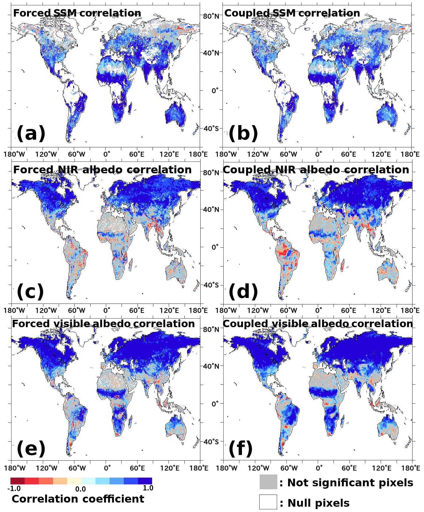
Figure 3 Spatial patterns of the correlation coefficient along time series (with monthly time steps) per pixel for SSM and albedo. (a, b) Correlation coefficient between simulated SSM and CCI-SSM in normalized VWC for forced and coupled mode, respectively. (c, d) Correlation coefficient between simulated and observed (MODIS) albedo in NIR band for forced and coupled mode, respectively. (e, f) Those in visible band. White areas are null pixels that were excluded by the quality control, and gray areas are statistically not significant pixels.

The precipitation bias in forced mode is very small in most regions since the simulation relies on bias-corrected precipitation (WFDEI), which relies on the GPCC data set used here as reference data. Yet, it is not negligible everywhere (Fig. 2a), and the forced ORCHIDEE precipitation (WFDEI) is higher than GPCC in small tropical pockets, the US Great Plains, and boreal zones, which are prone to precipitation undercatch because of strong winds and/or a large fraction of snowfall (Becker et al., 2013). The largest precipitation biases in coupled mode, i.e., in absolute value, are found in the wettest areas (humid tropics) and mountain ranges (Fig. 2b), which is consistent with the analysis of Cheruy et al. (2020) in terms of bias sign and spatial pattern.

Figure 2c–d show that the spatial pattern of normalized SSM bias in forced and coupled modes are consistent and delineate the biased regions clearly. The strong negative biases in normalized SSM was observed over the boreal region (except eastern Siberia) with high SWE values (Fig. 1j), suggesting the relation to snow or permafrost. Note that satellite observation uncertainties in such snowy regions could also be a reason for the discrepancy. The farm belt of India and China (with a lot of irrigation in Fig. 1h) exhibits a systematic lower bias in SSM. Apart from those, arid (northern Africa, central Australia, and northern China) and tropical (the Congo and the Amazon basins) regions also showed lower correlation (Fig. 3a–c), part of which can be attributed to the inherent feature that CC tends to be low when the range in which the sample varies is narrow. To better identify the error sources in SSM, we plotted the mean seasonal cycles (i.e., monthly climatology) separately for each latitude zone (Fig. 4). Substantial parts of the time series were consistent between simulation and observation (except the grayed-out period due to insufficient sample size and low reliability of the reference data). The underestimated simulated SSM values compared to the CCI-SSM values in the summer season in 30–60^∘ N (Fig. 4b) may be attributed to anthropogenic water input due to irrigation because this region includes large-scale agricultural fields (Fig. 1h). In the low-latitude regions, the simulated values tend to underestimate SSM in the dry season and to show larger seasonal change (Fig. 4c, d). Most of the areas exhibited small ET biases in absolute value (Fig. 2e, f), suggesting that ORCHIDEE is highly capable of representing global ET. The coupled simulation tended to simulate larger ET values than the forced simulation did, which can be explained to some degree by the larger mean precipitation in the coupled simulation than that in the forced one (as shown by the larger positive bias for the coupled simulation in Table 3). Regions with large ET biases were distributed in the tropical (the Amazon and the Congo basins and the maritime continent), mountainous (the Rockies, Andes, and Himalayas), and agricultural (especially in India) regions. Mountainous regions tended to be characterized by a positively biased precipitation in the coupled simulation (Fig. 2b), which caused a positive ET bias (especially in North and South America). Tropical regions exhibited complex responses in ET between the coupled and forced simulations. The maritime continent (Indonesia and the other tropical Pacific islands) had negative ET biases for both simulations. The Congo basin and a large part of the Amazon basin exhibited contrasting patterns between the simulations (the uncoupled one had a negative bias, whereas the coupled one had a positive bias). The link between ET and precipitation in the coupled simulation was only straightforward in the Congo basin, where the positively biased precipitation (water input) led to a positive bias of ET. In a part of the maritime continent, the coupled ET was negatively biased despite a positive bias of precipitation. Conversely, the coupled ET was positively biased in the Amazon basin despite a negative bias of precipitation.

Table 3 Land averages of the evaluation criteria (bias, RMSE, and CC) for the selected variables and reference data sets. The same bias on the average over land for all variables was observed between forced and coupled simulations. Positive systematic bias was observed for LAI, and a large uncertainty (i.e., RMSE) was observed for SSM and ET. ET shows the best correlation coefficient. Overall, the coupled simulation tends to behave more realistically, despite the overestimation of precipitation.

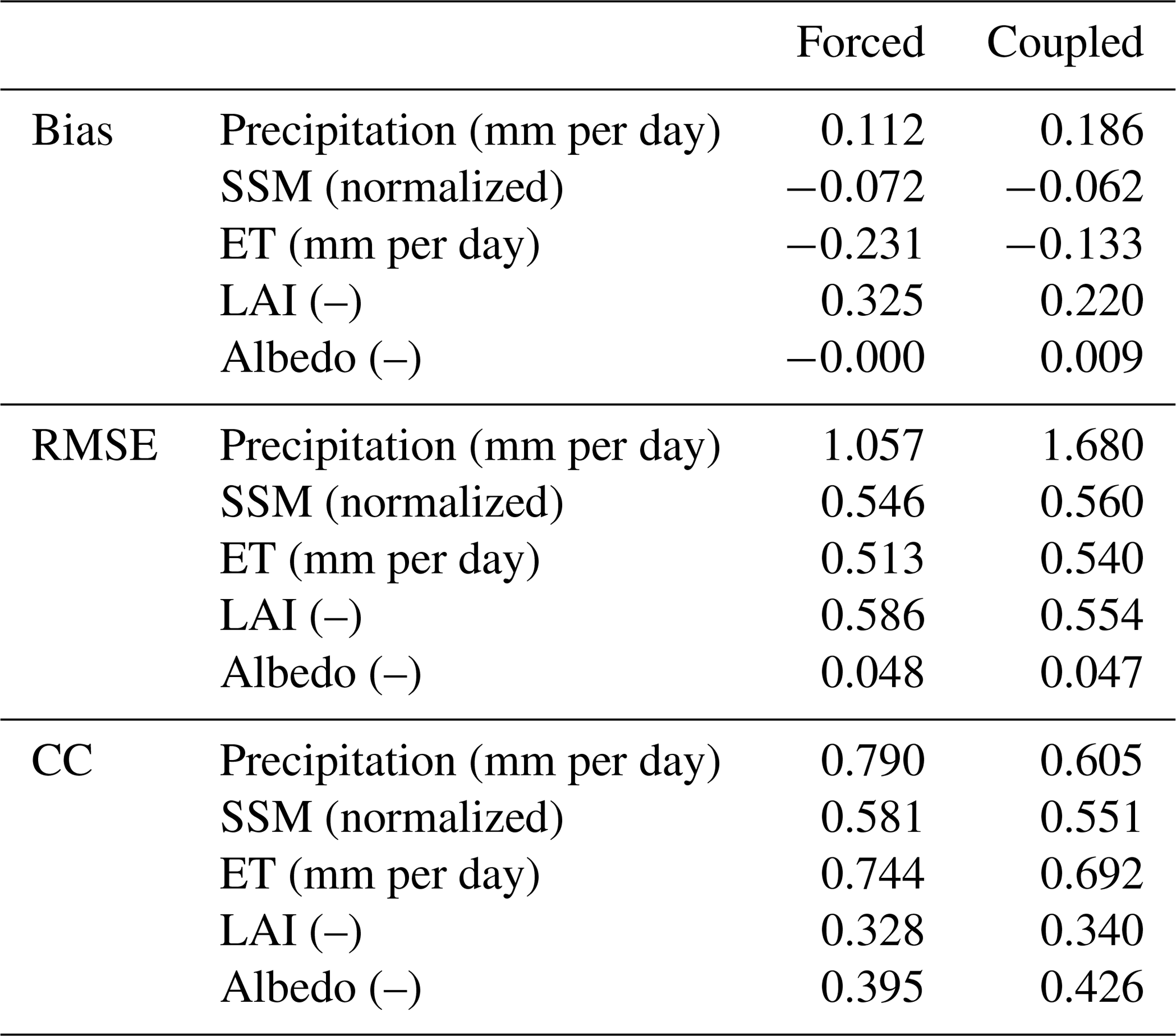
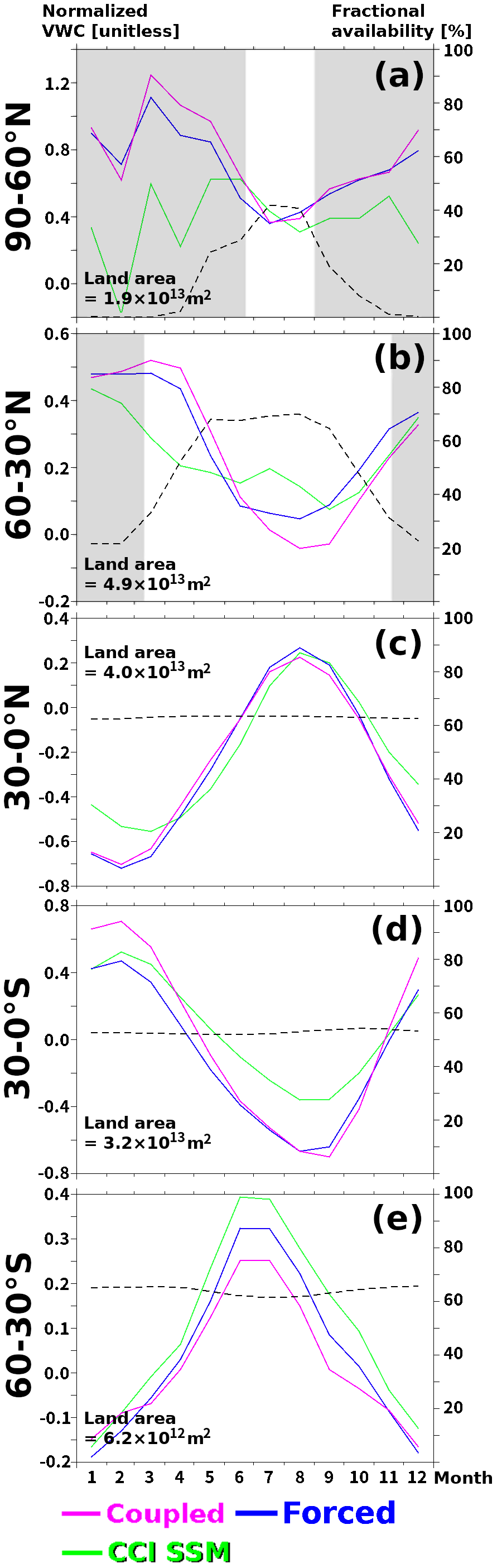
Figure 4 Comparison of SSM seasonal variations among reference (CCI-SSM) and simulations (forced and coupled) for each latitude zone. The dashed black line is the fraction of available pixels to all land pixels over each zone. Depending on the snow mask, the number of available pixels varied along the season in high-latitude regions. To avoid a misleading interpretation, a small number of samples with unreliable SSM reference and periods of less pixel availability (< 30 %) are grayed out.

Positive bias of LAI was observed in large areas globally (Fig. 2g, h). Given the strong similarity between the forced and the coupled bias maps, it is suggested that the bias comes mostly from the surface component, such as PFT maps, or the reference data. In fact, LAI retrievals by space-borne sensors like MODIS may be saturated for large values of LAI (Zhao et al., 2016), resulting in an underestimation of LAI in reference. Despite such a positive bias tendency, the boreal region in eastern Siberia, the shores of the Great Lakes in North America, and the basin of the Mekong River all exhibited negative bias of LAI. In addition, there were hot spots of negatively biased LAI in such regions as the Zambezi River system lying across Angola and Zambia. Contrasting biases between the simulations were observed around the Himalayas.

In most regions, the simulated bias for total albedo was small, and the bias patterns were generally similar between the forced and coupled modes (Fig. 2i, j). The largest biases were the overestimation in the mountainous regions (especially the Himalayas in the coupled mode) and the underestimation in the boreal and polar regions, where snow affects the albedo. In addition, simulated and observed albedo were uncorrelated (or negatively correlated) in many regions apart from the boreal one (Fig. 3c–f). Low correlation coefficients in the arid and tropical region can be attributed to the temporal invariance of the land surface. However, even in some temperate and semi-arid zones where temporal variance is likely to be high, low correlation was observed. In such regions, seasonal changes in the land surface (caused mainly by vegetation phenology and the snowfall/snowmelt cycle) may not be described well in ORCHIDEE. In fact, the global monthly climatology (Fig. 5a, f) showed that global mean NIR albedo was overestimated all year long, except in the spring when visible albedo was underestimated. The main source of the NIR albedo overestimation seemed to come from the temperate zone (30–60^∘ N; Fig. 5c), suggesting overestimated vegetation cover (having high reflectance in NIR spectral region) there from summer to autumn. There was a systematic overestimation of albedo in the tropical band (Fig. 5d, e, i, j), and a small underestimation in the snow-related season (winter to spring) of the boreal band (Fig. 5b, g).

Figure 5 Monthly climatological time series of global and zonal mean albedo. The left column shows the NIR band (a – global average; b–e – zonal average for each 30^∘ in latitude), while the right column (f–j) shows the visible band (the vertical arrangement is the same as that for NIR).

3.2 Factor analysis

The bivariate linear regressions between simulated ECV bias and factors (Table 4) and the box plots against each factor class (Figs. 6–8) firstly reveal a large bias variability within each class, resulting in a large part from the spatial variability of the simulated variables across the various climates and biomes of the globe. However, some controls could be identified despite this variability. It is particularly the case for irrigation, which has an obvious impact on the simulated hydrological variables (SSM, ET, LAI, and precipitation; Fig. 6a, c, e, and g). Both the coupled and forced models show negatively biased values in the largely irrigated areas (classes 5 and 6), except for the forced-mode SSM. This is understandable because the simulations overlook irrigation, which creates artificial water input to the soil, resulting in additional ET and plant growth in reality. Interestingly, the coupled simulation underestimates the observed values more than the forced one does (Fig. 6a, c, e, and g), which probably relates to a positive feedback driven by surface–atmosphere coupling (Mahfouf et al., 1995; Liu et al., 2003; T. Wang et al., 2015). Since the forcing WFDEI precipitation is based on in situ rain gauges which integrate the impact of the real-world irrigation, this factor has a relatively weak effect in the forced mode.

Table 4 Spatial correlation coefficients (SCCs) between biases (in forced and coupled modes) and potential explanatory factors. PFT was excluded here because it is on a nominal scale. Statistically insignificant SCCs appear in italics. SSM tended to be underestimated in high P, SSM, ET, and LAI regions for both forced and coupled modes. Between forced and coupled ET, an opposite association with P, ET, and LAI was observed. LAI in both modes was positively biased in high P, ET, and SSM regions (probably corresponding to the tropical region). Albedo and coupled P were strongly associated with slope. Irrigation is likely to bias SSM and ET negatively, and the effect was more enhanced in the coupled mode.

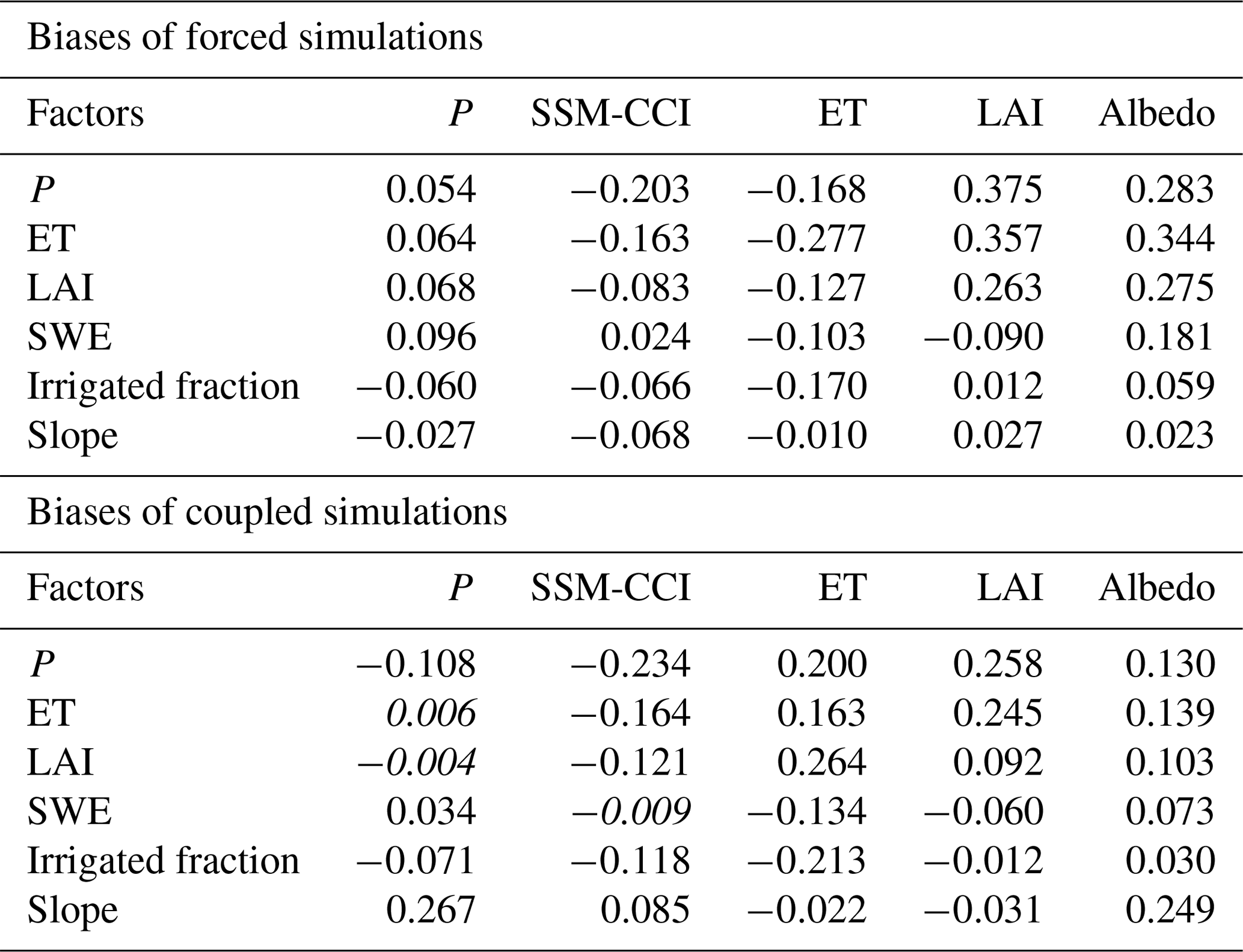
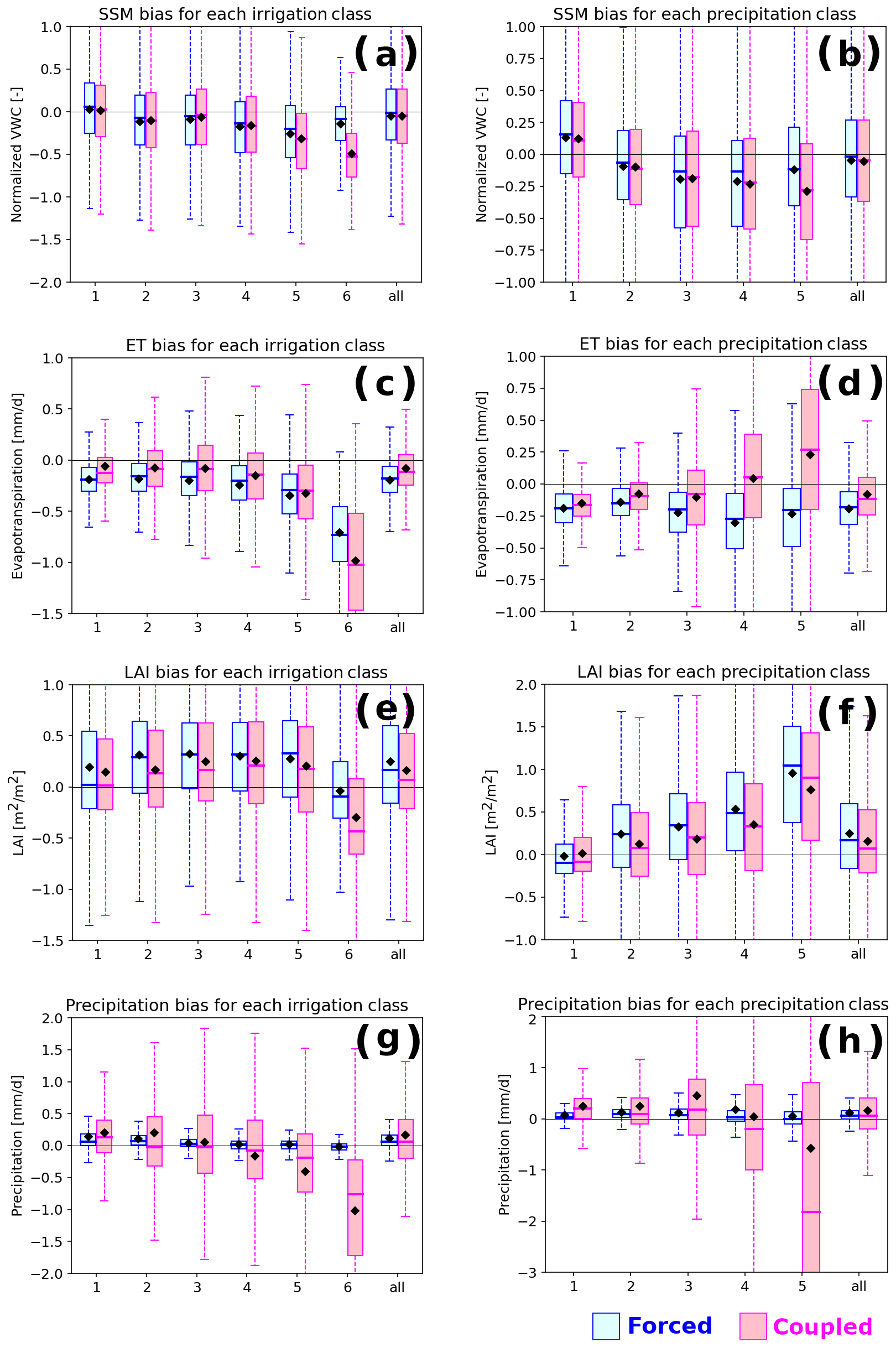
Figure 6 Box plots of mean biases (simulated minus observed values) of SSM, ET, LAI (forced/coupled), and precipitation (coupled only) against each class of irrigation and precipitation. The upper limit, middle line, and lower limit of the boxes correspond to 25, 50, and 75 percentile values, respectively. The upper and lower limits of whiskers are maximum and minimum values, respectively. The diamond indicates the mean value of the class. (a, b) SSM bias. (c, d) ET bias. (e, f) LAI bias. (g, h) Precipitation bias vs. irrigation and precipitation classes, respectively. Blue and pink boxes correspond to forced mode and coupled mode, respectively. The horizontal black line shows zero. Each class of landscape factors (i.e., x axis) is defined in Table 1.

The contrasting ET bias pattern between forced and coupled modes in the Congo and the Amazon basins (Fig. 2e, f) was also confirmed in the factor analysis of precipitation (classes 4 and 5, which probably correspond to tropical regions; Fig. 6d), PFT (class 2 – broadleaf evergreen in Fig. 7a), LAI (class 3 in Fig. 7b), and ET (class 3 in Fig. 8a). This also explains the contrasting correlation sign of ET bias with P, SSM, ET, and LAI in Table 4.

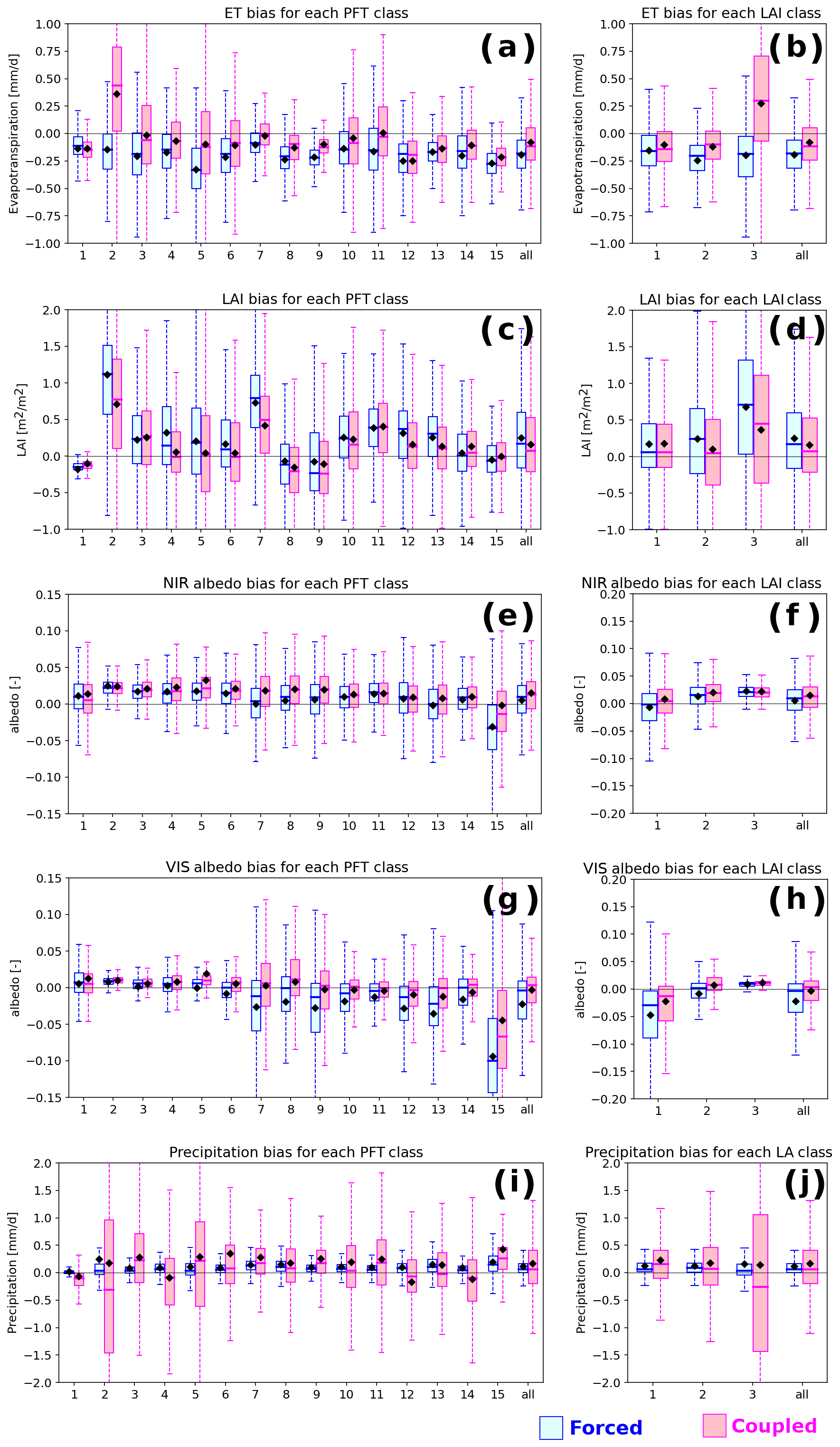
Figure 7 Box plots of mean biases (simulated minus observed values) of ET, LAI, NIR/visible albedo (forced/coupled), and precipitation (coupled only) against each class of PFT and LAI. (a, b) ET bias. (c, d) LAI bias. (e, f) NIR albedo bias. (g, h) Visible albedo bias. (i, j) Precipitation bias vs. PFT and LAI classes, respectively. Legends and axes are the same as in Fig. 6, and each class of landscape factors (i.e., x axis) is defined in Table 1.

Figure 8 Box plots of mean biases (simulated minus observed values) against each class of ET, slope, and SWE. (a, b) ET and LAI bias vs. ET class. (c, d, e) NIR albedo, visible albedo, and precipitation bias vs. slope class. (f, g) NIR and visible albedo bias against SWE class, respectively. Legends and axes are the same as in Fig. 6, and each class of landscape factors (i.e., x axis) is defined in Table 1.

The factor analysis confirms the positive bias of LAI in the tropical regions, which are characterized by high precipitation (classes 4 and 5 in Fig. 6f), broadleaf evergreen forest (PFT 2 in Fig. 7c), high LAI (class 3 in Fig. 7d), and high ET (class 4 in Fig. 8b). However, some of the positive bias in such tropical regions might be compensated by the negative bias of the simulated precipitation (especially in the Amazon; Fig. 2b, also confirmed by class 3 in Fig. 7j), resulting in a smaller bias of LAI in the coupled simulation than that in the forced simulation. Negative LAI bias in the boreal region is also confirmed by the PFT factor analysis (classes 8, 9, and 15 in Fig. 7c). Eastern Siberia is the main place with negative LAI biases (Fig. 2g, h). Possible explanations include persistent snowpack reducing the vegetation growing season, underestimated maximum LAI in the model, and errors in the reference LAI product, especially at high latitudes, due to the less reliable assessment of solar reflectance from space (Guimberteau et al., 2018).

For albedo, the effect appeared in the factor analysis against slope (class 3 in Fig, 8c and d) and SWE (classes 4 and 5 in Fig. 8f and g) as a discrepancy between the coupled and forced simulations. In the steep regions, the coupled simulation tended to be positively biased because of the precipitation bias. In the high SWE region, the negative bias of albedo was enhanced in the forced simulation. This is due to the already mentioned compensation of the positive bias in the mountainous region with the negative bias in the boreal and polar regions (Fig. 2i, j). The NIR albedo in the tropical region (classes 2 and 3 in Fig. 7e and class 3 in Fig. 7f) tended to be slightly large for both simulations. This is consistent with the positive bias of LAI in such regions (Fig. 2g, h), although the range of bias was small.

4 Discussion

In general, the ORCHIDEE simulations show good spatiotemporal consistency with the reference data, except for issues related to external water addition/subtraction and surface–atmosphere coupling. An example of the external source of water input is irrigation. Largely irrigated areas obviously lead to underestimated hydrology-related model parameters (i.e., SM, ET, and LAI). Although the impact of irrigation on ORCHIDEE SSM simulation has been suggested by Yin et al. (2018) over a specific region (China), our experiment demonstrated explicitly that the effect on SSM in the forced mode is relatively small on the global scale and rather larger on ET and LAI (Fig. 6a, c, and e). Integrating the irrigation process in ORCHIDEE with an ancillary agricultural map and data assimilation (Raoult et al., 2019) may improve the accuracy (de Rosnay et al., 2003). Through the land–atmosphere coupling (Al-Yaari et al., 2019a), the impact of the irrigation is emphasized in the coupled simulation (Fig. 6a, c, e, and g), where strong negative bias was observed in not only ET, LAI, and precipitation but also SSM over largely irrigated areas. Specifically, a lack of description of the additional water input and artificial vegetation over irrigated agricultural land led to lower SSM and LAI, which, in turn, led to lower ET. In the coupled simulation, the lower SSM also led to lower humidity and lower precipitation, resulting in enhanced underestimation of SSM in the next time step (i.e., positive feedback). The enhanced SSM underestimation caused enhanced ET underestimation and enhanced LAI underestimation through the parameterizations of carbon assimilation and vegetation phenology. The underestimation of precipitation in the coupled simulation over irrigated areas (e.g., India in Fig. 2b; classes 5 and 6 in Fig. 6g) supports the validity of this emphasizing effect in the coupled model, which is consistent with other reports (Mahfouf et al., 1995; Liu et al., 2003; T. Wang et al., 2015). The spatial similarity between the bias maps of SSM, ET, and precipitation (Fig. 2a–f) over central and southern Africa, Australia, and a large part of southern and eastern Asia also suggests a strong interlink between them in coupled mode. A potential interpretation is that precipitation is the first-order control on SSM and ET in the region (i.e., water-limited ET). It also can be interpreted as a result from a positive feedback between precipitation, SSM, and ET in such regions, as reported by Yang et al. (2018).

However, other factors need to be considered regarding land–atmosphere feedback and their influence on coupled precipitation and ET. In particular, ET is not controlled solely by precipitation but also by radiation (Cheruy et al., 2020), and temperature determines the potential ET (Dirmeyer, 2001; Nasonova et al., 2011). The complex response of ET to precipitation in the present study suggests the importance of those factors. For example, there may be a negative feedback in the Amazon and the maritime continent between precipitation and ET because these areas are strongly energy limited (Seneviratne et al., 2010; McVicar et al., 2012). In the maritime continent, positive precipitation bias meant more cloud coverage than reality, which decreased the available energy and ET. In contrast, the negative precipitation bias in the Amazon meant less cloud coverage, larger available energy, and larger ET than in reality.

Although such feedback explains the overestimated ET in the Congo and the Amazon basins in the coupled simulation, it does not explain the underestimated ET in the forced simulation. Potential explanations are excessive water stress on ET, insufficient soil-water-holding capacity, underestimated precipitation or radiation in WFDEI, and/or an overestimation of ET by the Jung product in the regions of high precipitation. Conversely, too weak water stress in dry areas (either for transpiration or soil evaporation) can also explain the negative correlation between forced-mode ET bias and precipitation (Table 4). A solution could be to activate a resistance to soil evaporation, increasing with the top soil dryness (Cheruy et al., 2020). Such contrasting results between the forced and coupled modes imply the importance of model evaluation under both modes to isolate the potential error sources.

Compared with the forced mode, the positively biased precipitation simulated by the coupled mode may positively bias the albedo, particularly in the mountainous areas (high slope class in Fig. 8c–e) via considerable snow cover. This probably arose from an incomplete atmospheric simulation of the local climate (Cheruy et al., 2020), such as an updrift along a mountain slope. Coarse spatial resolution of the atmospheric simulation in the coupled mode can also make it difficult to represent the impact of mountainous topography on local climate (Decharme and Douville, 2006). Theoretically, the overestimation of albedo should decrease the available energy at the surface, thereby decreasing ET and surface temperature. The slight negative bias of ET in the Himalayas (Fig. 2f), despite the positive bias of precipitation (Fig. 2b), can be explained by the decrease in available energy due to the increased albedo (Fig. 2j). Such an ice–albedo interaction in the ORCHIDEE–LMDZ coupled mode has also been reported over the boreal region (T. Wang et al., 2015; particularly pronounced in spring temperature over eastern Siberia). Taking the ice–albedo feedback into consideration with the secondary factors (i.e., radiation and temperature) that affect ET, the link between precipitation and ET in the coupled mode is rather complex in the mountainous and boreal regions. Moreover, the deficit of available energy may reduce photosynthesis and, thus, vegetation growth, causing a peaky underestimation of LAI in the Himalayas in the coupled mode (Fig. 2h), which is not observed in the forced mode (Fig. 2g).

Part of the positive biases in normalized SSM in the eastern Siberia and polar region (Fig. 2c, d) may be attributed to freezing and snowmelt and related vegetation phenology, as excessively large or fast snowmelt occurs in the spring in ORCHIDEE (Fig. 5b, g). However, other control factors are likely involved in SSM overestimation, such as wetlands, permafrost, and albedo. The negative albedo bias found in the boreal zone (Fig. 2i, j) in spite of the positive snowfall bias (Fig. 2a, b) can also be explained by the excessive snowmelt. This underestimation of albedo in many boreal areas, also noted in Cheruy et al. (2020), was expected to lead to overestimated ET, but it did not lead to an obvious ET bias because of the underestimated LAI (Fig. 2g, h). Given the spectral features of land cover (Petty, 2006), the NIR albedo is related largely to an abundance of vegetation, i.e., LAI. Therefore, uncertainty in snow and LAI leads to uncertainty in the surface albedo, which further propagates uncertainty in the energy balance and water cycles. Such a complicated relationship should be treated in the special tuning of ORCHIDEE for high latitudes (Druel et al., 2017; Guimberteau et al., 2018). In addition to high-latitude regions, vegetation seasonality in the temperate zones seemed uncertain. In the temperate forests, the model is likely to simulate spring green-up that is considerable and/or very fast (Fig. 5c), which causes an overestimated NIR albedo and discrepancies in LAI and albedo seasonality.

Regardless of the origin (i.e., satellite, reanalysis, or in situ), observations inevitably contain inherent uncertainty, which leads to uncertainty in the model assessment. SSM retrieval over substantially high/low vegetation, tropical/arid regions, and highly heterogeneous and high-roughness regions remains challenging (Ma et al., 2019). Therefore, some part of the low SSM correlation in arid/tropical regions (Fig. 3a, b) can be attributed to uncertainties in the satellite products in addition to an inherent feature of CC. Snow cover and RFI (Oliva et al., 2012) may also cause uncertainties in satellite-based SSM estimation, although we attempted to remove such uncertain pixels by means of a preliminary quality check. Using multiple data sources (e.g., the Soil Moisture Active Passive (SMAP) product; Entekhabi et al., 2010) as references for model evaluation (Eyring et al., 2016b) is a promising way to address such uncertainties. A brief attempt with the SMOS-IC product (Fernandez-Moran et al., 2017) is shown in Fig. S8. Inconsistency between the model-simulated SSM depth (up to 10 cm) and the penetration depth of satellite sensors (several centimeters) may also cause uncertainties in the assessment, although using normalized SSM instead of absolute SSM is likely to mitigate the effect to some extent.

The satellite-based LAI product (Zhu et al., 2013) may be affected by the saturation issue of optical satellite data (i.e., MODIS) in regions with high LAI. The snow albedo of the MODIS product (MCD43) has a slightly larger uncertainty (RMSE ≈ 0.07; Stroeve et al., 2005, 2013) than that of the snow-free daily mean albedo (RMSE = 0.034; D. Wang et al., 2015). However, this does not alter our conclusion about the ORCHIDEE albedo uncertainty in the snow region, but some of the uncertainty might be attributed to the error in satellite observation.

We depended largely on satellite-derived data for the SSM, LAI, and albedo evaluations. By contrast, we used a FLUXNET-based product (Jung et al., 2019) for the ET evaluation, which has potential uncertainties arising from (i) the statistical upscaling process (model tree ensemble; Jung et al., 2009), (ii) the input data required in machine learning prediction, and (iii) the heterogeneous distribution of ground stations. Because the latter potential issue is particularly important for hardly accessible regions such as tropical and mountainous areas, progress in the data coverage of the FLUXNET network is desirable. Although ET products derived from satellite data (Miralles et al., 2011; Zhang et al., 2010; Zeng et al., 2014) can also be used, unlike the other variables (SSM, LAI, and albedo), the retrieval of ET is not done directly from the satellite observations but depends largely on the process-oriented models. Therefore, in addition to the uncertainties in the satellite observations themselves, such products have uncertainties that arise from ancillary data (e.g., atmospheric conditions and land cover) required in the model and from imperfections in the model structure/parameterization (a preliminary comparison among the different data sources can be found in Fig. S9).

The difference between the forced ORCHIDEE precipitation (WFDEI) and GPCC (Fig. 2a) probably comes from the undercatch correction based on Legates and Willmott (1990) for GPCC and on Adam and Lettenmeier (2003) for WFDEI. Schneider et al. (2014) acknowledge that, for the GPCC product, “the biggest uncertainty issue is the correction of the systematic gauge-measuring error (general undercatch of the true precipitation)”, but this is very likely true for all precipitation products.

Note that the present study is based on a specific LSM (i.e., ORCHIDEE 2.0), atmospheric model (i.e., LMDZ6A), and forcing data (WFDEI). Future work should include addressing the uncertainties that arise from the LMDZ model structure/parameterization and the resolution in the numerical simulation (Hourdin et al., 2013). Uncertainties that arise from the atmospheric model have been analyzed for ET and SSM by Cheruy et al. (2020). For China, forced ORCHIDEE simulations with WFDEI have been shown to perform better than with other forcing data sets (Princeton Global Meteorological Forcing and Climatic Research Unit – National Centers for Environmental Prediction; Yin et al., 2018). More generally, the uncertainty arising from atmospheric forcing selection should be kept in mind as it is comparable to the one of varying the LSM in forced simulations (Guo et al., 2006). Other perspectives include factor analysis against other hydrometeorlogical parameters such as radiation, temperature, and precipitation frequency (Qian et al., 2006; Yin et al., 2018).

5 Conclusions

This paper has presented an in-depth evaluation of five interlinked essential climate variables (namely surface soil moisture, evapotranspiration, leaf area index, albedo, and precipitation) simulated by ORCHIDEE land surface model under different simulation modes (either forcing by WFDEI or coupled with LMDZ). Statistical evaluation was conducted using various reference data sources (ESA CCI, upscaled FLUXNET, Global Inventory Modeling and Mapping Studies (GIMMS) 3g, MODIS products, and GPCC), and factor analysis was conducted against various landscape factors (namely plant functional type, leaf area index, irrigation, precipitation, slope, snow water equivalent, and evapotranspiration). Although ORCHIDEE consistently represented the spatiotemporal patterns of each essential climate variable in general, some issues were found relating to water cycles and their different consequences between the forced and coupled simulations. There were errors relating to freezing and/or snowmelt, artificial water input, such as irrigation, and precipitation bias propagated through surface–atmosphere coupling in the coupled mode. The factor analysis revealed a strong link between irrigation and precipitation (that further affected surface soil moisture, evapotranspiration, and leaf area index, particularly in the coupled mode) and a relatively complex link between precipitation and evapotranspiration that reflected the hydrometeorological regime of the region (energy limited or water limited) and the snow–albedo feedback in mountainous and boreal regions. In addition, the description of vegetation and snow seasonality seemed to be an issue in ORCHIDEE. Excessive and/or too fast green-up in temperate forest may lead an overestimation of leaf area index and near infrared albedo. Excessive and/or too fast snowmelt in spring in the boreal region may result in the underestimation of albedo in such regions, which can affect the energy balance and water cycles. The different results between the forced and coupled modes stress the importance of model evaluation under both modes to determine each potential error source in model simulation.