the Creative Commons Attribution 4.0 License.
the Creative Commons Attribution 4.0 License.
 | 16 Apr 2021
Global cotton production under climate change – Implications for yield and water consumption
Werner von Bloh
Sibyll Schaphoff
Christoph Müller
Being an extensively produced natural fiber on earth, cotton is of importance for economies. Although the plant is broadly adapted to varying environments, the growth of and irrigation water demand on cotton may be challenged by future climate change. To study the impacts of climate change on cotton productivity in different regions across the world and the irrigation water requirements related to it, we use the process-based, spatially detailed biosphere and hydrology model LPJmL (Lund–Potsdam–Jena managed land). We find our modeled cotton yield levels in good agreement with reported values and simulated water consumption of cotton production similar to published estimates. Following the Inter-Sectoral Impact Model Intercomparison Project (ISIMIP) protocol, we employ an ensemble of five general circulation models under four representative concentration pathways (RCPs) for the 2011–2099 period to simulate future cotton yields. We find that irrigated cotton production does not suffer from climate change if CO2 effects are considered, whereas rainfed production is more sensitive to varying climate conditions. Considering the overall effect of a changing climate and CO2 fertilization, cotton production on current cropland steadily increases for most of the RCPs. Starting from ∼65 million tonnes in 2010, cotton production for RCP4.5 and RCP6.0 equates to 83 and 92 million tonnes at the end of the century, respectively. Under RCP8.5, simulated global cotton production rises by more than 50 % by 2099. Taking only climate change into account, projected cotton production considerably shrinks in most scenarios, by up to one-third or 43 million tonnes under RCP8.5. The simulation of future virtual water content (VWC) of cotton grown under elevated CO2 results for all scenarios in less VWC compared to ambient CO2 conditions. Under RCP6.0 and RCP8.5, VWC is notably decreased by more than 2000 m3 t−1 in areas where cotton is produced under purely rainfed conditions. By 2040, the average global VWC for cotton declines in all scenarios from currently 3300 to 3000 m3 t−1, and reduction continues by up to 30 % in 2100 under RCP8.5. While the VWC decreases by the CO2 effect, elevated temperature acts in the opposite direction. Ignoring beneficial CO2 effects, global VWC of cotton would increase for all RCPs except RCP2.6, reaching more than 5000 m3 t−1 by the end of the simulation period under RCP8.5. Given the economic relevance of cotton production, climate change poses an additional stress and deserves special attention. Changes in VWC and water demands for cotton production are of special importance, as cotton production is known for its intense water consumption. The implications of climate impacts on cotton production on the one hand and the impact of cotton production on water resources on the other hand illustrate the need to assess how future climate change may affect cotton production and its resource requirements. Our results should be regarded as optimistic, because of high uncertainty with respect to CO2 fertilization and the lack of implementing processes of boll abscission under heat stress. Still, the inclusion of cotton in LPJmL allows for various large-scale studies to assess impacts of climate change on hydrological factors and the implications for agricultural production and carbon sequestration.
- Article
(1723 KB) - Full-text XML
-
Supplement
(4910 KB) - BibTeX
- EndNote


Being an extensively produced natural fiber on earth, cotton (Gossypium spp.) is providing income to millions of farmers. According to the World Bank Atlas (Sheth, 2017), 8 of the top 10 cotton-producing countries are classified as developing countries, and their exports of the crop reached ∼ USD 30 billion in 2017 (ITC, 2019) (full overview in Table S1). Particularly in the West African region – the world's third-largest cotton exporter (following North America and Central Asia) – cotton has played an important part in the economic development and has remained a key source of livelihood for many farmers (Hussein et al., 2005; Perret and Bossard, 2006). Worldwide, cotton is already broadly adapted to growing in temperate, subtropical, and tropical environments, but growth may be challenged by future climate change (Bange et al., 2016). Climate change is likely to affect cotton production both positively and negatively. Temperature influences cotton growth and development by determining rates of fruit production, photosynthesis, and respiration (Turner et al., 1986; Hearn and Constable, 1984).
However, the growth of cotton plants differs at varying stages of plant development and by plant organ (Burke and Wanjura, 2010), and thus a temperature optimum for cotton cannot be defined. Yield and growth of cotton are directly affected by a high temperature. Additionally, hot weather conditions increase the evaporative demand on cotton plants, leading to more intense water stress (Hall, 2000). Elevated atmospheric carbon dioxide concentrations ([CO2]) on the other hand are expected to increase cotton yields as cotton is a C3 crop (Kimball, 2016). Numerous free-air carbon dioxide enrichment (FACE) studies demonstrated a strong reaction of cotton yield and growth to an increased CO2 concentration (Kimball, 1983; Cure and Acock, 1986; Hileman et al., 1994; Hendrix et al., 1994; Reddy et al., 1997; Mauney et al., 1994; Bhattacharya et al., 1994). Likewise, water-use efficiency can be improved by CO2 enrichment because it increases biomass and causes partial stomatal closure at the same time, consequently reducing transpiration (Mauney et al., 1994; Hileman et al., 1994; Broughton, 2015; Ko and Piccinni, 2009).
Crop models have been used to assess the effect of changing climate conditions on crop productivity, but the main focus has been on major staple crops – such as maize, wheat, rice, and soybean (e.g., Challinor et al., 2014; Rosenzweig et al., 2014; Müller et al., 2015; Pugh et al., 2016; Schleussner et al., 2018) – that provide the majority of calories to human nutrition (Yahia et al., 2019; Welch and Graham, 2004).
The response of other crops has been assessed less thoroughly, despite their importance for economies or human nutrition. With this study, we aim to examine the impacts of climate change on cotton productivity in different regions across the world. We therefore add cotton as an additional crop to the global dynamic vegetation, hydrology, and crop growth model LPJmL (Lund-Potsdam-Jena managed land) version 4.0 (Schaphoff et al., 2018b). We provide an evaluation of model skill by comparing simulated cotton yields to yield statistics (FAO, 2018). To study climate change impacts on future cotton productivity, we simulate future cotton yields and related irrigation water requirements under a set of future climate scenarios (Hempel et al., 2013), following the Inter-Sectoral Impact Model Intercomparison Project (ISIMIP) protocol (Warszawski et al., 2014).
2.1 The LPJmL model
The global dynamic vegetation model LPJmL is a well-established and thoroughly evaluated model (Schaphoff et al., 2018b, a; Müller et al., 2017) that is unique in combining natural vegetation, hydrology, and managed ecosystems (croplands, pastures) in one consistent framework for gridded large-scale applications. The model has been extensively described by Schaphoff et al. (2018b), and we here only provide a short summary of the most relevant features for this study and the extensions implemented for cotton. Agricultural crops have been implemented as annual crops with daily computation of photosynthesis, autotrophic respiration, evapotranspiration, and allocation of assimilates to plant organs (Bondeau et al., 2007). Individual crops are grown on separate spatial units (stands) within each grid cell so that different crops do not compete for water and light, mimicking monocultures. Also purely rainfed and irrigated crop cultivation can be simulated on separate stands, and irrigation water can be applied by different irrigation techniques and can be limited by actual freshwater availability (Jägermeyr et al., 2015). LPJmL – here operated at a 0.5 arcdeg spatial resolution – simulates processes underlying the growth and productivity of both natural and agricultural vegetation (Sitch et al., 2003; Bondeau et al., 2007; Lapola et al., 2010; Rolinski et al., 2017). The model represents 10 plant functional types (PFTs) as well as 12 crop functional types (CFTs) and 3 bioenergy plantation systems (Beringer et al., 2011). In LPJmL, carbon, water, and energy fluxes are closely linked to reproduce plant growth dynamics and to account for the effects of changes in climate conditions and water availability (Gerten et al., 2004, 2007). Several features – such as river routing (Rost et al., 2008a), irrigation systems (Jägermeyr et al., 2015), a soil hydrological and carbon distribution scheme (Schaphoff et al., 2013), and a fire module (Thonicke et al., 2010) – further improved the model. The calculation of photosynthesis is based on the Farquhar model (Collatz et al., 1991; Haxeltine and Prentice, 1996; Sitch et al., 2003). Water consumption is ruled by plant physiology, and the coupling between vegetation and water cycle enables the separation of productive (transpiration) and unproductive (interception, evaporation) portions of plant water use. Moreover, water flows are divided into green (precipitation) and blue (irrigation) water (Rost et al., 2008b; Jägermeyr et al., 2015, 2016). The evaluation of various model components – e.g., crop yields, evapotranspiration, and river discharge – has shown that LPJmL is a tool suitable for analyzing changes in vegetation and water. Schaphoff et al. (2018a) provide a comprehensive evaluation of the LPJmL model.
2.2 Implementation and parameterization of cotton
Twelve crop types are already implemented in LPJmL (temperate and tropical cereals, pulses, maize, rice, temperate and tropical roots, sunflower, soybeans, groundnut, rapeseed, sugar cane) (Bondeau et al., 2007; Lapola et al., 2010). In this study we include cotton, which was originally implemented as a perennial crop in LPJmL by Fader et al. (2015) for the Mediterranean region. However, in most parts of the world, cotton is cultivated as an annual crop (Ritchie et al., 2007; Whitaker et al., 2018). We modify the modeling approach developed by Fader et al. (2015) accordingly and implement cotton into LPJmL version 4.0 (Schaphoff et al., 2018b) as an annual crop. Similar to Fader et al. (2015), the cotton plant is simulated and parameterized as an agricultural tree, and we calculate phenology and growth on a daily basis (see below). We adopt most of the key parameters used by Fader et al. (2015) and adjust values for plant density and temperature optimum for photosynthesis (Table 1). Other than adjusting these two parameters, we did not calibrate any plant growth parameters. To account for regional differences, we use country-specific planting densities provided by several studies (Sect. 2.2.2). As the intensity of irrigation on irrigated cotton-producing areas in the different production regions is unknown, we conduct simulations with different levels of deficit irrigation (25, 50, 75, and 100 % of required irrigation water) and select the irrigation level that produces the cotton yield that is closest to observations (Sect. 2.3). In this study, simulated cotton yields should be understood as the entire cotton fruit, that is, both cotton lint and cottonseed.
Table 1Key parameters of cotton according to Fader et al. (2015).

Values marked with an asterisk (*) were adjusted. Kest: tree density range; HR: harvest ratio; Tb: base temperature; Phopt: optimum temperature range for photosynthesis; Tlim: lower and upper coldest monthly mean temperature; WCF: conversion factor (moisture content) from dry to fresh matter.
2.2.1 Phenology and growth
Wild cotton is a deciduous perennial tree, and the fruiting habit of the plant is not clearly established; i.e., vegetative and reproductive growth occur at the same time (Ritchie et al., 2007). During the growing period the leaves supply photosynthates to plant growth and the developing fruit and are shed only when the plant is stressed such as during drought, disease, nutrient starvation, or frost (Wullschleger and Oosterhuis, 1990). The perennial nature of cotton, even its modern cultivars, is not helpful in achieving high yields of cotton lint and seed. Consequently, through breeding and changes in cultivation practices, cotton is now farmed as an annual crop to prevent diseases and optimize cotton production (Ritchie et al., 2007; Whitaker et al., 2018). Once the entire crop is mature, the leaves serve no useful purpose, and their removal can be beneficial for mechanical harvesting. Crop maturity is characterized by slowed development of new main-stem nodes, causing first-position white flowers to appear progressively closer to the plant apex (Oosterhuis et al., 1993). The development of cotton plants is particularly sensitive to temperature, leading to an acceleration of all stages of phenological development (Bange et al., 2001; Hodges et al., 1993; Reddy et al., 1997). However, being an indeterminate plant, the phenological phases of cotton cannot be clearly distinguished and represented as a function of temperature (Bange et al., 2016), and the growing period is thus not necessarily shortened by warming as, e.g., observed in annual crops.
To account for the current production system, cotton is implemented in LPJmL as small agricultural trees that are planted annually and removed at the end of the growing period, representing the annual production mode.
The phenology – i.e., the temporal dynamic of the canopy greenness – is computed with the growing season index concept as described and parameterized by Forkel et al. (2014). The daily phenology status is determined by multiplying limiting effects of cold temperature, short-wave radiation, water availability, and heat stress. Thus, vegetation greenness is limited by temperature-induced heat stress. The saplings are initialized with 2.3 gC of sapwood and a leaf-area index of 1.6 m2 m−2. Similar to phenology, gross primary production (GPP) and net assimilation (NPP) of cotton plants are calculated daily. Increasing daily air temperature values lead to a higher respiration (maintenance) rate, which can exceed carbon assimilation, resulting in a negative NPP (Schaphoff et al., 2018b). Fruit growth is expressed as daily carbon accumulation (Cfruit) of a fraction of NPP after square set, i.e., as soon as squares (pre-bloom fruiting buds) emerge. The development of squares indicates the initiation of a fruiting branch. The model implementation assumes that cotton fruit growth occurs after the fractional cover of green leaves has reached 60 % of full leaf cover, i.e., when the phenology scaler phen =0.6. This follows the description of Ritchie et al. (2007) on the canopy and fruit development of cotton plants.
where HR is the harvest ratio and NPP the daily net primary productivity of the tree. On days with negative NPP, fruit growth is halted, but accumulated yield is not reduced, reflecting the fact that boll development dominates plant growth at this stage of reproductive growth (Ritchie et al., 2007). At the end of the growing period, cotton harvest H is determined as
where the day of square set (DS) and harvest day (DH) define the length of the simulated reproductive period.
A possible simultaneous establishment of herbaceous PFTs in the same areas of agricultural trees, representing grasses and weeds (for modeling details see Schaphoff et al., 2018b), can be simulated by LPJmL but was turned off in the simulations here. This mimics effective weed control, mainly practiced in cotton farming today to reduce competition for water and nutrients (Ritchie et al., 2007; Whitaker et al., 2018).
2.2.2 Specification of planting densities, sowing dates, and irrigation
A country-specific planting density (kest) is used as model input, which is, apart from irrigation and sowing dates, the only management aspect that is explicitly considered. These country-specific planting densities have been taken from the literature (Abdullaev et al., 2007; Iqbal et al., 2012; Venugopalan et al., 2013; Dong et al., 2006; Bednarz et al., 2006; Zhi et al., 2016; Khan et al., 2017; Bozbek et al., 2006; Echer and Rosolem, 2015; Dai and Dong, 2014; Vaughan, 2005; Akhtar et al., 2002) and are shown in Fig. S1. The cotton-specific planting density parameter (plants m−2 a−1) was introduced similar to the annual establishment rate kest of PFT individuals (Schaphoff et al., 2018b).
The growing season of cotton plants is prescribed from the sources specified in Sect. 2.3. Thereby the sowing date defines the start of the growing period and ranges between Julian day 1 and 335 of the year of sowing. The prescribed growing season length varies from 153 to 243 d for cotton plants to reach harvest.
Five hydrologically and thermally active layers represent the soil profile in LPJmL where roots access water, depending on their PFT/CFT-specific root distribution (Schaphoff et al., 2018b). The soil water content of the first layer determines the infiltration rate, and water not infiltrated forms the surface runoff. Similar to the infiltration approach, the percolation rate is limited by soil moisture of the lower layer, and excess water above saturation feeds the lateral runoff (Schaphoff et al., 2013).
Cotton is produced in rainfed or irrigated systems, whereas irrigation generally serves to reduce the impacts of rainfall deficits and thus reduces interannual yield variability. However, the actual amount of water applied to fields is unknown and determined by water availability, water management systems, and economic rationale. The extent to which rainfall deficits are compensated for by irrigation is thus not only a question of equipment for irrigation (Portmann et al., 2010), and water stress can still affect interannual yield variability in irrigated systems. In order to test the importance of deficit irrigation for cotton production, we performed several runs, varying the fraction of soil pore space filled up in individual irrigation events from 0 (corresponding to purely rainfed conditions) to 1 (meeting full irrigation demand) by increments of 0.25.
If the soil water content in the upper 50 cm of the soil falls below 90 % of field capacity, an irrigation event is triggered. Soil water lower than atmospheric water demand requires a daily net irrigation (NIR, millimeters). NIR is calculated as the amount of water needed to fill soil water up to field capacity Wfc in the upper root layers of the soil.
where wa is the soil water in millimeters actually available.
Inefficiencies of different irrigation systems cause additional water needs to meet crop water demand. For that reason, LPJmL considers conveyance efficiency (Ec) and calculates application requirements (AR) for each system. Consequently, the gross irrigation requirement (GIR; millimeters) – i.e., the amount of water requested for abstraction – results in
where Store is a storage buffer. The storage buffer is filled up with available irrigation water not used due to available precipitation and is released in the next irrigation event. A detailed explanation about the computation of NIR, GIR, and Store in LPJmL is given in Rost et al. (2008b) and Jägermeyr et al. (2015). The application requirements are calculated as
where Wsat is the soil moisture content at saturation level (in mm); DU is an irrigation system-specific scalar (no unit), to distribute irrigation water uniformly across the field, and wfw is the available free water (in millimeters) (Jägermeyr et al., 2015). Note that the computation of GIR is relevant for simulations in which irrigation water is constrained by available river discharge and reservoir capacity (e.g., Jägermeyr et al., 2015) but not here, where we assume explicit levels of deficit irrigation but no additional constraints on water limitation.
This model development is based on LPJmL4, a model version that does not account for nutrient limitations, and, thus, fertilizer effects are not considered.
2.3 Modeling protocol, input, and reference data
All simulations are conducted at a 0.5∘ longitude–latitude grid resolution with daily weather input data and annual data on atmospheric carbon dioxide concentrations ([CO2]). To simulate historical results, we ran the LPJmL model for the period 1901–2011 using the Climate Research Unit's TS 3.23 monthly data for temperature, wet days, and cloudiness (Harris et al., 2014) and precipitation data (Version 5) provided by the Global Precipitation Climatology Centre (Rudolf et al., 2011). Monthly weather input data are converted to daily data, using an internal weather generator (Schaphoff et al., 2018b). Data on [CO2] refer to records at the Mauna Loa station (Tans and Keeling, 2015). A 120-year spin-up (recycling the first 30 years of input climatology) preceded transient runs to bring water fluxes and soil temperatures into dynamic equilibria. As soil carbon pools have no effect on cotton productivity in this version of the model, a longer spin-up to correctly initialize soil and vegetation carbon pools (Schaphoff et al., 2018b) is not necessary here. Simulations for future periods are conducted for four different representative concentration pathways (RCPs) – RCP2.6, RCP4.5, RCP6.0, and RCP8.5 (Moss et al., 2010) – each implemented by five different general circulation models (GCMs): GFDL-ESM2M (Dunne et al., 2012, 2013), HadGEM2-ES (Jones et al., 2011), IPSLCM5A-LR (Dufresne et al., 2013), MIROC-ESM (Watanabe et al., 2011), and NorESM1-M (Bentsen et al., 2013), which have been bias-corrected as described by Hempel et al. (2013). Data on [CO2] for future periods are taken from the corresponding RCP data sets (Moss et al., 2010) as provided by the ISIMIP project (Frieler et al., 2017). To assess how cotton plants respond to future climate change, we ran the model for the time span 1951–2099, again preceded by a 120-year spin-up period. The averaging time for historical yields differs (depending on the purpose) and is indicated for each figure. Future yield projections are presented as 2070–2099 averages, compared to annual means averaged over the reference period 1980–2009, or as full time series. The spatial distribution of cropland dedicated to cotton was taken from the land-use data set MIRCA2000 (Portmann et al., 2010), which provides both rainfed and irrigated harvested areas around the year 2000 with a spacial resolution of 5 arcmin (Fig. S2).
Sowing dates and growing period were provided as gridded model input, combining sowing and harvest information provided by the ICAC's World Cotton Calendar (WCC) (Committee, 2014) and Portmann et al. (2010). More precisely, we used the WCC data and filled gaps with data offered by MRICA (Fig. S3). Because increasing temperatures do not necessarily shorten the period of growth for cotton plants (Bange et al., 2010; Luo et al., 2014a) and parameterization of cotton partly reflects more advanced cultivars (Sect. 2.2), we here assume that the growing season length remains static in all simulations.
Cotton yield levels modeled under different irrigation options on irrigated cotton areas (Sect. 2.2.2) were compared with national yield levels published by FAO (2018), reported as “Seed cotton” there. Since LPJmL is a global model, we evaluated the model at the global and national level. However, on the grid cell level simulated cotton yield results were also tested against semi-controlled field experiments. For these comparisons management assumptions (sowing and harvest dates, planting densities) were adapted to reproduce experimental conditions (Fig. S8).
3.1 Evaluation of model performance
In order to evaluate the performance of this extended LPJmL model version, simulated historical cotton yields are compared to observed data (Fig. 1) published by FAOSTAT (FAO, 2018). The modeled cotton yield levels are in good agreement with reported values. Statistical analyses for both the top 10 cotton-producing countries and cotton-growing countries in West Africa show that simulated national yield levels can reproduce reported national yield levels well (Fig. 1). For the top 10 cotton-producing countries, cotton yields simulated under full irrigation often match FAO values best. The whiskers that depict the range of yield levels simulated with different irrigation options on the irrigated cotton cropland often reach the zero line, indicating that cotton production in these countries (Pakistan, Turkmenistan, Turkey, Uzbekistan, etc.) is not possible without irrigation. National yield levels can also be reproduced well in West Africa, where in contrast to the top 10 producer countries hardly any irrigated cotton production exists (Fig. S2). An overview of the model performance for all cotton-growing countries is given in the Supplement, Table S2.
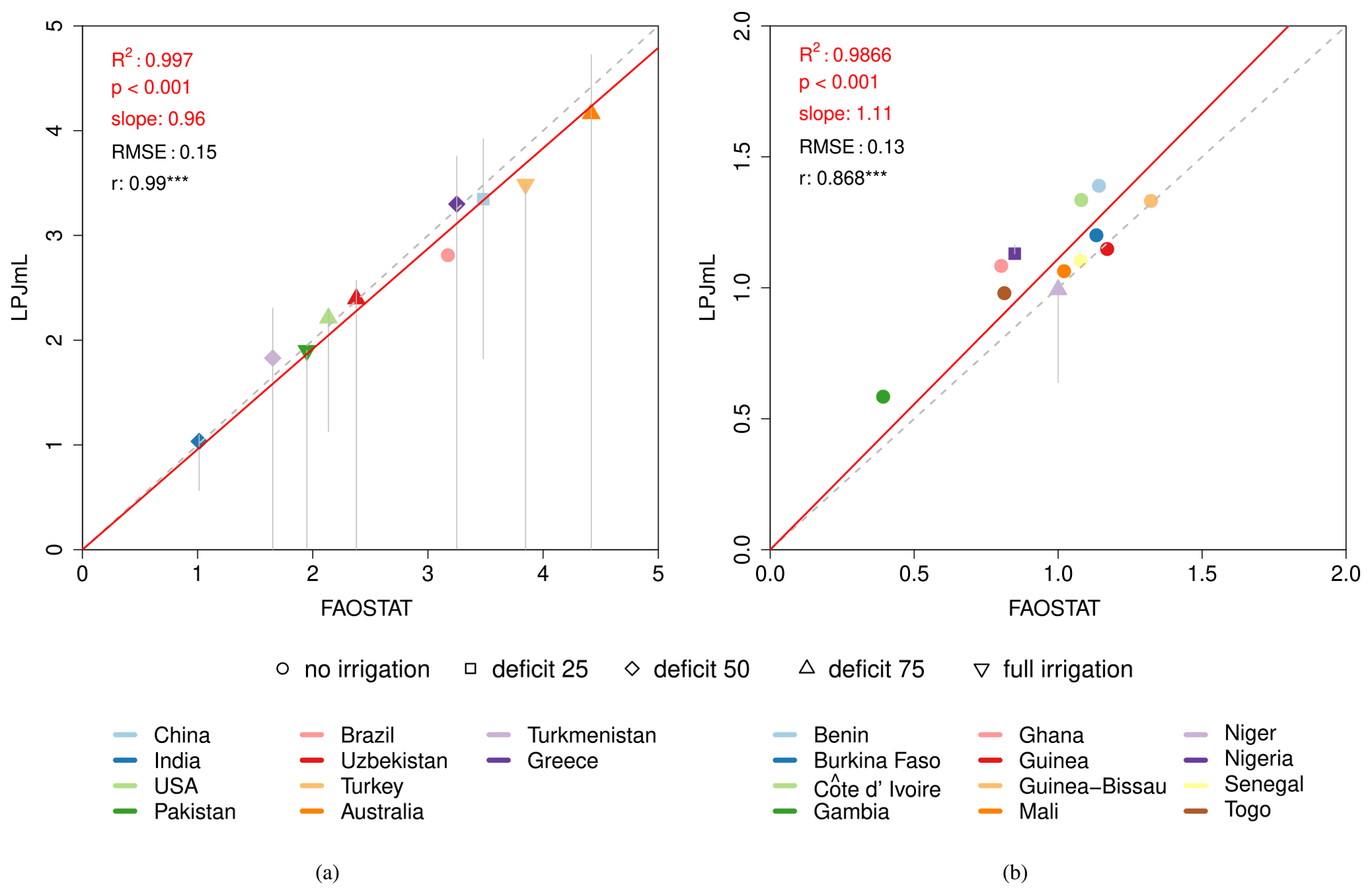
Figure 1Comparing simulated cotton yields [t ha−1] to observed values for (a) the top 10 cotton-producing countries and (b) West African countries. Whiskers indicate the yield range of different irrigation options on irrigated cotton cropland in these countries (Portmann et al., 2010). LPJmL yield data and FAOSTAT yield data were both averaged over the time period 2000–2009.
For these simulations, the planting densities in LPJmL have not been calibrated against observed yield levels but are based on reported planting densities (Fig. S1). The model simulations can reproduce statistically significant shares of reported variability in time of intensely managed top producing countries, such as the USA and Australia as well as a few West African countries (Figs. 2 and S4) and other countries (Table S2). The model also reproduces some of the historical interannual variation in global cotton production (Fig. 3). The spatial pattern of cotton yields is shown in Fig. S5.
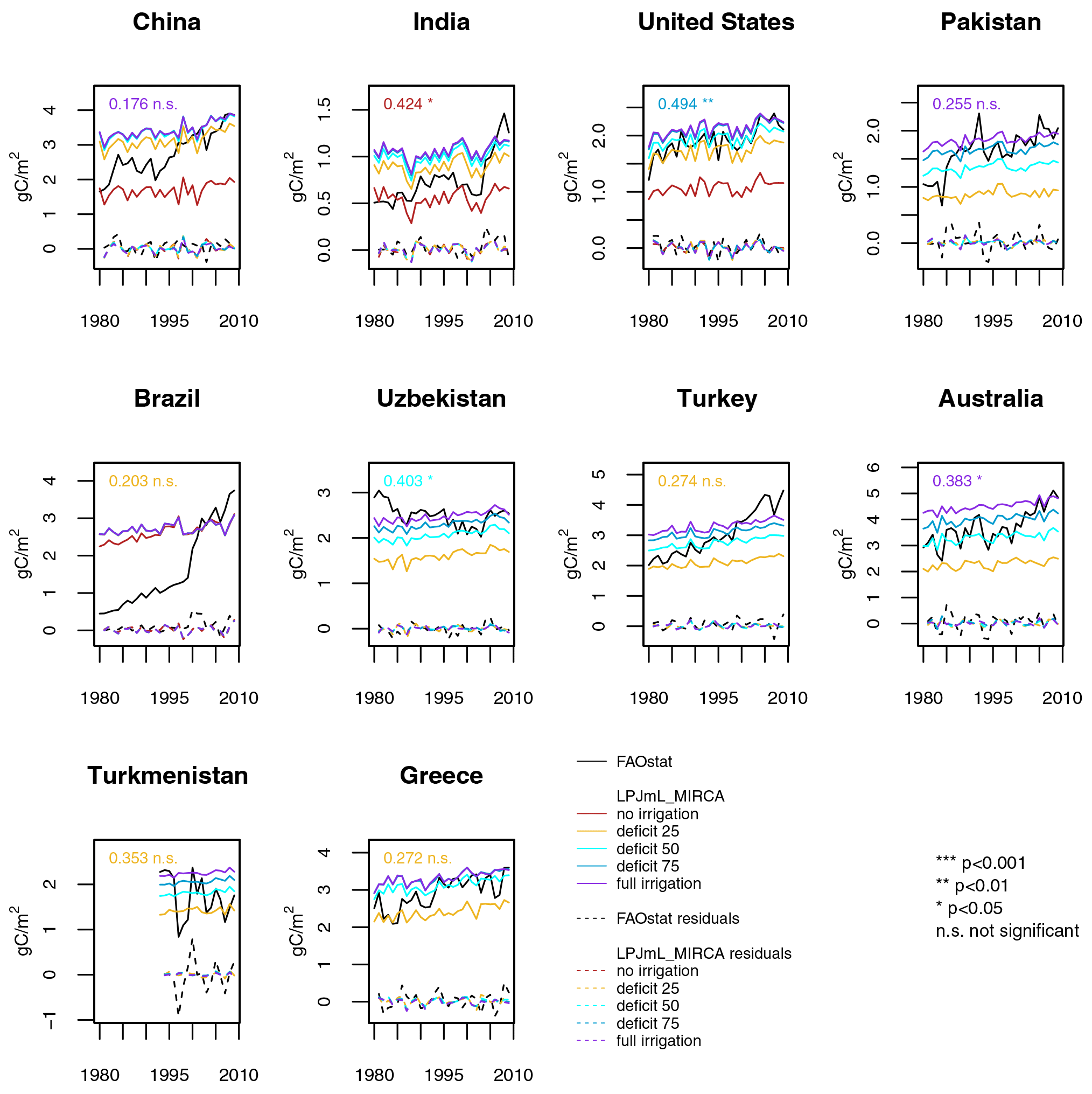
Figure 2Comparing interannual yield variability for the top 10 cotton-producing countries. Numbers in each plot depict the correlation coefficient between simulated residuals and FAOSTAT residual data. The different irrigation options (on irrigated cropland only) are shown in colored lines. The color of the correlation coefficient indicates the best-fitting irrigation option. For Turkmenistan, yields have only been reported from 1992 onward (FAO, 2018), so only these years are shown in the plot.
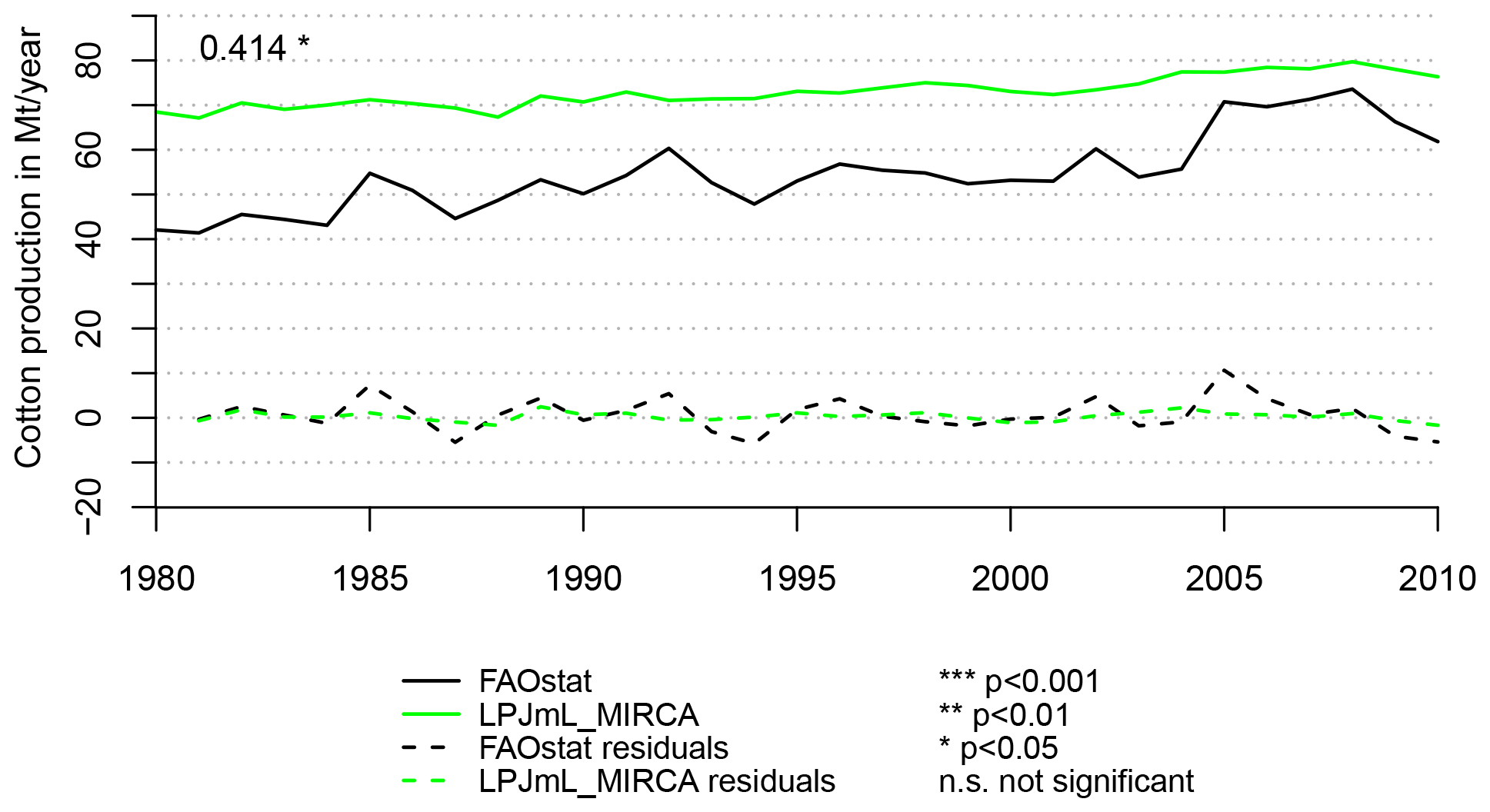
Figure 3Time series of historical global cotton production [million tonnes per year]. The number in the plot depicts the correlation coefficient between simulated residuals and FAOSTAT residuals.
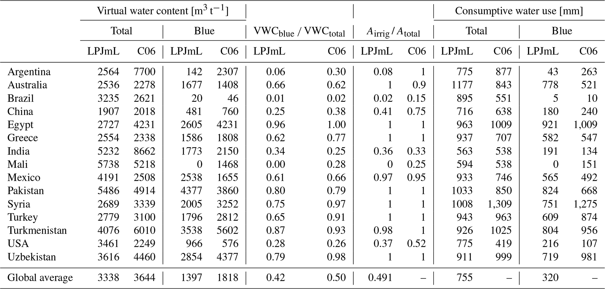
We further evaluate the model results with respect to the water consumption of cotton production against data provided by Chapagain et al. (2006), averaged over the time period 1997–2001. For reasons of comparability, we therefore followed the concept of “virtual water content” (Allan, 1997, 1998) and calculated the virtual water content of cotton (tonnes per meter) as the ratio of the water (green and blue in cubic meters per hectare) used to grow a crop in the field to the related crop yield (tonnes per hectare). We find that LPJmL simulations of water consumption of cotton production are in good agreement with the estimates of Chapagain et al. (2006) with respect to the order of magnitude and spatial variability (Fig. S6 and Table 2). The virtual water content is quite variable across regions and mainly in an inverse relation of the yield pattern (Fig. S5), suggesting that spatial yield variability is higher than the spatial variability in actual evapotranspiration. As virtual water content is a criterion for water-use efficiency (Hoekstra, 2003; Hoekstra and Mekonnen, 2012; Zhuo and Hoekstra, 2017), moderate values in regions with high irrigation shares (compare Figs. S6 and S7) point to an efficient use of (blue) water. The efficiency of blue-water use depends on management practices – such as irrigation techniques, irrigation strategies, and mulching practices (Gleick, 2003; Perry, 2007; Perry et al., 2009; Zhuo and Hoekstra, 2017) – to reduce non-beneficial losses (soil evaporation) as well as on other yield-reducing factors, such as nutrient limitations or pests. In the Indo-Gangetic plain, drip irrigation of cotton is only applied in experimental fields, and farmers grow cotton by applying irrigation water through flood irrigation (Thind et al., 2008; Aujla et al., 2008). Here, the water consumption of cotton production is at the high end, indicating substantial non-beneficial water losses (Thind et al., 2010).
Table 2Virtual water content and consumptive water use for cotton production in the major cotton-producing countries for the period 1997–2001. Reference data taken from Chapagain et al. (2006), here referred to as C06. VWCblue: blue virtual water content; VWCtotal: total virtual water content; Airrig: irrigated harvested cotton area; Atotal: total harvested cotton area.
For the evaluation of the modeled cotton yield response to elevated [CO2], we compare simulated yield effects to those reported from open-top chamber (OTC) and FACE experiments. Kimball (2016) report strong yield increases in cotton bolls under elevated [CO2] (∼38 %), which is a stronger yield response than most other crops. Experimental data from Kimball et al. (1992) and Mauney et al. (1994) also show that the level of water and nutrient availability affects the relative cotton yield response to elevated [CO2]. Similarly, LPJmL yields also result in a strong response depending on the level of [CO2] increase and water stress (see Fig. S8). Observational data are only available for one OTC site (Phoenix, AZ, USA) and one FACE site (Maricopa, AZ, USA), so it remains unclear how the cotton yield response to elevated [CO2] varies across different climate zones and management regimes. However, the range of simulated yield increases under elevated [CO2] seems to be often adequately reproduced by LPJmL in the corresponding grid cells (Fig. S8).
3.2 Climate change impacts on cotton production
Considering the overall effect of climate change and CO2 fertilization, future cotton productivity slightly increases – starting from ∼65 million tonnes in 2010 – until 2040 for all RCPs similarly by ∼10 %. For RCP2.6, global cotton production on current cropland slightly declines after 2040, while for the remaining RCPs simulated production on current cropland steadily increases. Looking at RCP4.5 and RCP6.0, cotton production equates to 83 and 92 million tonnes at the end of the century, respectively. Under RCP8.5, simulated global cotton production rises by more than 50 % up to 102 million tonnes by 2099 (Figs. 4 and S9 for relative changes).
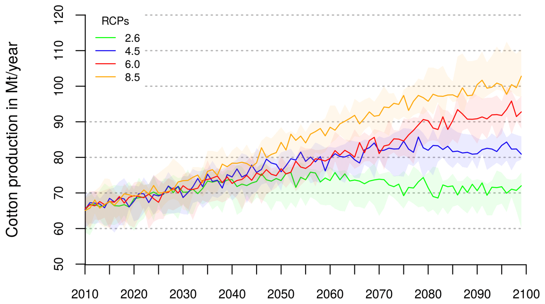
Figure 4Simulated global cotton production [million tonnes] for different RCPs. Transparent colors show the uncertainty ranges of five different GCM patterns.
Spatial patterns of projected changes in cotton yields (Fig. S10) show that increases are mainly expected in cooler or irrigated environments (Fig. S2), but exceptions exist, such as Pakistan and northern India, where cotton yields are projected to only slightly increase despite irrigation. Overall, the spatial patterns of projected yield increases seem to be quite static but scale with the emission scenario (RCP, Fig. S10).
The projected increases in yield are the result of interacting processes, which are often dominated by a positive response to elevated [CO2]. Higher temperatures initially stimulate cotton plant growth by accelerating phenological processes and thus reaching full canopy closure earlier in the season. If, however, high temperatures persist throughout the growing season, phases of plant stress (heat and water stress) emerge earlier and then reduce leaf cover and halt the reproductive growth of cotton plants. This yield-decreasing effect of climate change is masked by the strong growth-stimulating effect of elevated [CO2] (see Figs. S11 and S12 for simulations with static [CO2], where yields continuously decline with increasing climate change).
Without the beneficial effect of elevated [CO2], climate change leads to yield declines in most of the current cotton production area (Fig. S13). Across all RCPs the spatial variation of impacts shows a diverse pattern, resulting in climate-only-induced yield losses up to 2 t ha−1 in large parts of the cotton production area. Projected cotton yields for the high-end emission scenario (RCP8.5) decline significantly in Bolivia, Argentina, Iraq, Syria, and Egypt. Considerable losses are also projected for the USA, Brazil, India, Pakistan, Central Asia, the southeastern part of China, and Australia if no effects of CO2 fertilization are assumed. Only for Peru, northeast China, and some parts of Central Asia do the simulations project sustained cotton yield gains under climate change only.
3.3 Climate change impacts on irrigation water consumption
While changes in atmospheric CO2 may turn into enhanced water use or water-use efficiency of cotton production, the impact of elevated CO2 on cotton growth depends also on plant water availability. The simulation of future virtual water content of cotton grown under elevated CO2 results for all scenarios in less virtual water content compared to ambient CO2 conditions (Fig. 5). While there is only a slight decrease in virtual water content of cotton under RCP2.6, this effect is continuously strengthened across the emission scenarios (RCPs) for both well-watered and water-stressed conditions. Under RCP6.0 and RCP8.5, virtual water content is notably decreased by more than 2000 m3 t−1 in areas where cotton is produced under purely rainfed conditions, e.g., in West Africa and India. By 2040, the average global virtual water content for cotton declines in all scenarios from currently 3300 to 3000 m3 t−1 (Fig. S14a). Thereafter it slightly increases again under RCP2.6, while reduction continues for the remaining scenarios until the end of the century. The most considerable decrease by 30 % results in 2100 under RCP8.5 (Fig. S14b). The projected reduction of VWC of cotton is predominantly caused by increased cotton productivity, not by a reduction in cotton water consumption, i.e., the amount of water evapotranspired in cotton fields. Global cotton water consumption slightly increases from currently ∼235 km3 by 3.6 and 3 % at the end of the century under RCP2.6 and RCP8.5, respectively.
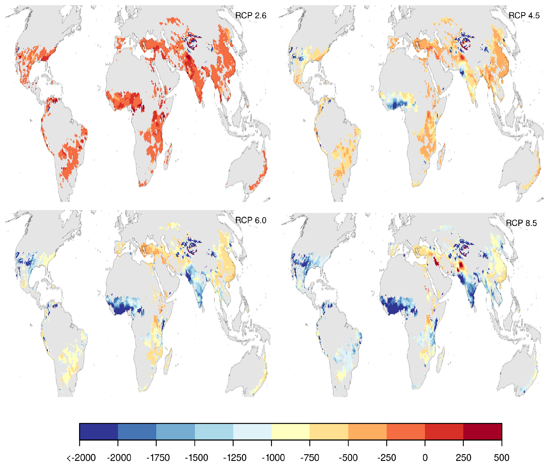
Figure 5Simulated changes in virtual water content of seed cotton [m3 t−1] for different RCPs. The spatial pattern of rainfed and irrigated cotton harvested areas was kept constant at the pattern of the year 2000 as provided by Portmann et al. (2010). Gray indicates areas currently not used for cotton production. Values were averaged over the five GCM patterns and over the period 2070–2099. Baseline period for comparison: 1980–2009.
While the virtual water content improves by the CO2 effect, elevated temperature (and water stress) acts in the opposite direction. Except for RCP2.6, the global virtual water content of cotton increases slightly but steadily under RCPs until mid-century. For RCP4.5 and RCP6.0 this development continues, resulting in a virtual water content roughly 10 % above the current value by 2100 (Fig. S15b) if no CO2 effect is assumed. The most obvious alteration is projected for RCP8.5, where the changing climate without accounting for the CO2 effect leads to an average global virtual water content of more than 5000 m3 t−1 by the end of the simulation period (Fig. S15a). The spatial pattern reveals that in all scenarios the virtual water content increases in all regions if CO2 effects are not accounted for. However, most drastic changes occur again in West Africa and India, where also the strongest changes are observed when CO2 effects are accounted for. While the CO2 effect leads to decreasing virtual water content in these regions, it increases by 2000 m3 t−1 if the CO2 effects are not accounted for (Fig. S16). Although cotton production strongly declines if the CO2 effect is neglected, increased VWC values clearly impinge on global water consumption of cotton production. For RCP2.6 and RCP8.5, the evapotranspiration related to cotton plantations amounts to 244 km3 (3.7 %) and 251 km3 (6.5 %) in 2100, respectively.
4.1 Model performance
The model can reproduce national yield levels very well (Fig. 1). This can in part be expected as we use the best-performing level of deficit irrigation in the comparison as well as national planting densities and reported growing seasons. However, overall yield levels are often not very sensitive to smaller changes in irrigation levels (full vs. deficit 75), and it is plausible to assume that irrigation typically is applied in quantities that are sufficient to eliminate the majority of water stress. Also, yield levels in countries with no or little irrigation can also be well reproduced. National planting densities have been taken from literature sources and were not selected to match observed yield levels. A wide range of (national) cotton planting densities is reported in the literature, which would allow for further modification of this parameter to refine our results. However, field research has shown different effects of increasing plant density on cotton yield, and to understand how cotton growth is affected by that parameter multiple interacting factors must be considered (Heitholt and Sassenrath-Cole, 2010). In this study, we therefore have selected planting densities corresponding to the lower end of the spread reported and kept these values static, but the literature suggests that planting densities have changed over time, explaining part of the temporal variation in cotton yields (Venugopalan et al., 2013). Another key component is the cultivar choice as several breeding programs have developed high-yielding cotton varieties well adapted to different environmental conditions (e.g., Bange and Milroy, 2004; Stiller et al., 2004, 2005; Bibi et al., 2008b).
The temporal variation in cotton yields can only partly be reproduced. This comparison is hampered by using static management assumptions in the absence of good spatially and temporally resolved management data, which is a general difficulty in evaluating gridded crop models' performance (Müller et al., 2017). The contribution of weather variability to yield levels remains unclear as the yield variability in reported yield statistics is affected not only by variability in weather but also by varying management conditions (Schauberger et al., 2016). Ray et al. (2012) reported that only 30 % of global yield variability can be attributed to weather drivers for maize, wheat, rice, and soybean, and Müller et al. (2017) also found better agreement between crop model simulations and yield statistics in high-input countries, suggesting that agreement between crop model simulations and yield statistics can only be expected in countries where management conditions are stable. Larger jumps in yield statistics as, e.g., in Brazil, China, India, Pakistan, and several West African countries suggest changes in management that cannot be expected to be reproduced by this modeling setup with static management assumptions (Dong et al., 2005; Venugopalan et al., 2013; Rossi et al., 2004). Additionally, inconsistencies between different data sets used to determine agricultural areas dedicated to cotton (details in Fader et al., 2015) cause significant deviations from the annual harvested cotton areas provided by FAO (2018), which was also reported as a source of uncertainty for other crops (Porwollik et al., 2017).
The good agreement with Chapagain et al. (2006) on virtual water content of cotton production adds further trust to the model simulations, as productivity and water consumption are intrinsically coupled in the model. Even though the estimates from Chapagain et al. (2006) are also model-based estimates rather than observations, the simulated patterns are plausible and have been achieved with different methods.
4.2 Implications of climate impacts
Elevated [CO2] has been shown to increase leaf photosynthetic rates and crop radiation-use efficiency (Hileman et al., 1994; Idso and Idso, 1994; Reddy and Zhao, 2005; Broughton, 2015) and reduce transpiration at the leaf level through reduced stomatal conductance (Hileman et al., 1994; Broughton, 2015; Zhao et al., 2004) in cotton. Both effects potentially lead to improvements in growth and yield. A broad range of yield increases, averaging around 38 %, has been reported for cotton bolls for an increase in [CO2] of 190 ppm (360 to 550 ppm), which is substantially stronger than the average response in most other crops, but only based on a very small set of experiments (Kimball, 2016). In line with changes in transpiration rates for canopies under elevated [CO2], Mauney et al. (1994) reported increased water-use efficiency as a function of increasing biomass production rather than a reduction in water use in the FACE experiments. In contrast, Reddy et al. (2005b) showed that increases in temperatures above optimum decrease cotton yield due to increased boll abscission and smaller boll size. In their experiment, even a significant increase in [CO2] did not fully compensate for the negative effects on yields. The authors concluded that future increases in [CO2] in combination with higher temperatures will decrease regional cotton yields. Likewise Reddy and Zhao (2005), Bibi et al. (2008a), Oosterhuis and Snider (2011), and Soliz et al. (2008) have shown cotton yields to be negatively impacted by elevated temperature (direct climate change). This is in line with our findings, except for Peru and northeast China, where we find that current yields are maintained under climate change. This is likely because present temperatures are considerably below the growth optimum and evaporative demand remains comparably low in the climate change scenarios considered here. In our model simulations, CO2 fertilization overcompensates for climate-change-induced yield penalties, and, although CO2 effects on cotton yields are largely unclear, FACE data support a strong positive effect (Hileman et al., 1994; Idso and Idso, 1994; Reddy et al., 1999; Mauney et al., 1994; Mauney, 2016). Even though Kimball (2016) do not report any results on CO2 fertilization effects under limited N supply, the co-limitation by nutrients is not covered here, and future research should account for these effects as well, e.g., by implementing these cotton features into the model version LPJmL5.0 that was developed in parallel (von Bloh et al., 2018). As with high air temperature (above 35 ∘C) the abscission of bolls increased sharply, leading to a boll retention close to zero at 40 ∘C (Reddy et al., 1991, 2005a; Zhao et al., 2005; Luo et al., 2014a), the performance of LPJmL on cotton yields could be enhanced by introducing a yield penalty depending on high temperature, e.g., a zero boll harvest index at temperatures above 35 ∘C. In this study, the upper optimum temperature limit constrains photosynthesis at 32 ∘C, indirectly inhibiting yield gain. However, decreasing crop yields caused by high temperatures are often a consequence of temperature-triggered water stress (Schauberger et al., 2017; Schlenker and Roberts, 2009), which is reflected in our model by an increased crop water demand.
Cotton is a perennial, indeterminate crop, and cultivated species are generally photoperiodic insensitive. Consequently, warmer temperatures will increase the rate of plant development but not necessarily reduce the length of growing season if temperature seasonality is the limiting factor (Waha et al., 2012; Minoli et al., 2019) and sufficient water and nutrients are available (Bange and Milroy, 2004; Wang et al., 2008; Stiller et al., 2004; Luo et al., 2014a; Bange et al., 2016). Hence, one major effect that reduces crop yields in annual crops (Ottman et al., 2012; Asseng et al., 2015) is not as relevant for cotton. However, cotton management decisions, such as actively shortening the season for growing cotton (Constable and Bange, 2015), were not accounted for.
Climate change is associated with changes in patterns of precipitation and water availability; hence, cotton plants in some regions may be subjected to plant water deficits. Water deficit limits growth and productivity of cotton plants, and the severity of the problem may increase due to changing world climatic trends (Le Houérou, 1996). Plant water deficits depend on both the supply of water to the soil and the evaporative demand of the atmosphere. Changes in atmospheric [CO2] may alter the water-use efficiency of cotton production. Cotton grown under [CO2] of 700 ppm uses water more efficiently compared with plants grown at a CO2 concentration of 350 ppm (Reddy et al., 1995, 1998; Ephrath et al., 2011) because closing the stomata to reduce the transpiration rate does not impede the same penalty on carbon assimilation under elevated [CO2]. Samarakoon and Gifford (1995, 1996) also found higher water-use efficiencies for cotton grown at [CO2] of 710 ppm than at ambient [CO2] (352 ppm) but demonstrated a higher plant water use compared with cotton grown at ambient [CO2] since increased biomass outpaced the water savings at leaf level. FACE experiments, however, showed no differences in total plant water use – i.e., evapotranspiration – of cotton grown at 550 ppm and ambient [CO2] (Dugas et al., 1994; Kimball et al., 1994; Hunsaker et al., 1994). Total water consumption (evapotranspiration) can thus be expected to respond to leaf biomass (canopy development), water-use efficiency, and water availability.
Our results suggest that the beneficial effects of elevated [CO2] on cotton yields overcompensate for yield losses from direct climate change impacts (temperature rise, changes in precipitation). Even though experimental evidence supports strong CO2 effects on cotton and it is plausible to assume that cash crops such as cotton are grown with sufficient fertilizer applications if economically feasible, several caveats remain. First, there are only very few data on cotton grown under elevated [CO2], so the modeled response remains inherently uncertain, especially in different climate zones and at high [CO2], which typically has not been investigated in experiments. Second, negative effects of heat days with temperatures above 35 ∘C are not represented in the model. Possible negative effects on crop phenology, such as the shedding of leaves under conditions of heat and/or drought, are not sufficiently understood and are also not represented in the model. Large shares of current cotton production areas are irrigated, and we find that irrigated cotton production does not suffer from climate change if CO2 effects are considered, whereas rainfed production is more sensitive to climate change. However, climate change also affects water availability for irrigation and thus has the potential to also substantially affect agricultural production (Elliott et al., 2014). These effects are not considered here, as the ISIMIP protocol for agricultural production prescribes unlimited water supply for irrigation (Frieler et al., 2017). Considering these caveats, our results need to be considered optimistic. Further research on the effectiveness of long-term and high-end CO2 fertilization effects as well as damages from heat is necessary to better constrain results. Accounting for constraints in freshwater availability is feasible with LPJmL in further research, yet many confounding effects, such as impacts from ozone (Schauberger et al., 2019) or pests and diseases, cannot be easily considered.
Overall, our simulation of climate change impacts on global cotton production results in patterns similar to other crops. Given the economic relevance of cotton production in areas such as West Africa or South Asia, climate change (elevated temperature and water stress effects) poses additional stress and deserves special attention. This holds particularly true as agriculture in these regions is already under pressure from increased demand for intensification considering rapid population growth. Changes in virtual water content and water demands for cotton production are of special importance, as cotton production is known for its intense water consumption that led, e.g., to the loss of most of the Aral Sea (Glantz, 1999; Pereira et al., 2009).
The implications of climate impacts on cotton production on the one hand and the impact of cotton production on water resources (with major impacts particularly in India and Uzbekistan) on the other hand illustrate the need to assess how future climate change may affect cotton production and its resource requirements. The inclusion of cotton in LPJmL allows for various large-scale studies to assess impacts of climate change on hydrological factors and its implications for agricultural production and carbon sequestration.The limited availability of data (such as valid information on tree density, irrigation management, and sowing dates) substantially limits model performance and evaluation. Another issue related to data scarcity is the need for scenarios of future cropping patterns, adaptation, and management as a consequence of climatic and socioeconomic change. With climate change very likely affecting the potential growing areas of cotton (as for other agricultural crops) and their profitability, it is essential to provide crop yield estimates and associated water requirements under different climate scenarios to other research projects, e.g., on land-use change projections (Nelson et al., 2014). Analyzing future cotton production may require a more detailed parameterization of cotton production, allowing for the differentiation of cotton varieties; grid-cell-specific planting densities and its differentiation between irrigated and rainfed conditions; and a crop-specific fruit set, which at present depends on the phenological development. The extended version of LPJmL is an important improvement as it allows for explicitly studying cotton production under climate change and associated water consumption. Results need to be carefully assessed and interpreted, as model performance remains uncertain under given constraints on data availability for model evaluation. Future work should focus on effects of climate change on irrigation water availability as well as on an implementation of heat stress effects on cotton productivity.
As the most widely produced natural fiber, cotton is of high importance to economies, but the growth of and irrigation water demand on cotton may be challenged by future climate change. To study how future cotton productivity is affected by projected climate change, we use the global biogeochemical model of hydrology, carbon exchange, and crop growth, LPJmL, expanded to include cotton plants. Available data on observations and published estimates are used to validate the model, and a set of climate scenarios following the ISIMIP protocol are used to simulate global future cotton yield and water consumption. We then analyze the global cotton production and irrigation water consumption under spatially varying present and future climatic conditions. Our results suggest that the beneficial effects of elevated [CO2] on cotton yields overcompensate for yield losses from direct climate change impacts, i.e., without the beneficial effect of [CO2] fertilization. While changes in atmospheric CO2 may turn into enhanced water use or water-use efficiency of cotton production, the impact of elevated CO2 on cotton growth also depends on plant water availability. The extended version of LPJmL is an important improvement as it allows for explicitly studying cotton production under climate change and associated water consumption. Our results should be regarded as optimistic, because of high uncertainty with respect to CO2 fertilization and the lack of implementing processes of boll abscission under heat stress. Thus they need to be carefully assessed and interpreted, as model performance remains uncertain under given constraints on data availability for model evaluation. Future work should focus on effects of climate change on irrigation water availability as well as on an implementation of heat stress effects on cotton productivity.
The model code of LPJmL4 is publicly available through PIK's GitHub repository at https://github.com/PIK-LPJmL/LPJmL and should be cited as Schaphoff (Ed.), S., von Bloh, W., Thonicke, K., Biemans, H., Forkel, M., Gerten, D., Heinke, J., Jägermeyr, J., Müller, C., Rolinski, S., Waha, K., Stehfest, E., de Waal, L., Heyder, U., Gumpenberger, M., and Beringer, T.: LPJmL4 Model Code. V. 4.0, GFZ Data Services, https://doi.org/10.5880/pik.2018.002, 2018. An extended, exact version of the code and the output data from the model simulations described here is published via GFZ Data Services at https://doi.org/10.5880/Pik.2020.001 and should be referenced as Jans (Ed.), Y., von Bloh,W., Schaphoff, S., and Müller, C.: LPJmL4 model code and model output for: Global cotton production under climate change – Implications for yield and water consumption. GFZ Data Services, https://doi.org/10.5880/Pik.2020.001, 2021.
The supplement related to this article is available online at: https://doi.org/10.5194/hess-25-2027-2021-supplement.
YJ and CM designed the study. YJ and WvB developed the model code, and YJ performed the simulations. YJ prepared the manuscript with contributions from all co-authors.
The authors declare that they have no conflict of interest.
We thank Jens Heinke and Susanne Rolinski for valuable discussions.
This research has been supported by the Bundesministerium für Umwelt, Naturschutz und Reaktorsicherheit (grant no. 16_II_148_Global_A_IMPACT).
The publication of this article was funded by the
Open Access Fund of the Leibniz Association.
This paper was edited by Pieter van der Zaag and reviewed by Kokou Adambounou Amouzou and one anonymous referee.
Abdullaev, I., Giordano, M., and Rasulov, A.: Cotton in Uzbekistan: water and welfare, in: The Cotton Sector in Central Asia – Economic Policy and Development Challenges, The School of Oriental and African Studies, London, UK, 112–128, 2007. a
Akhtar, M., Cheema, M. S., Jamil, M., Farooq, M. R., and Aslam, M.: Effect of plant density on four short statured cotton varieties, Asian Journal of Plant Sciences, 1, 644–645, 2002. a
Allan, J. A.: “Virtual water”: a long term solution for water short Middle Eastern economies?, School of Oriental and African Studies, University of London, London, UK, 1997. a
Allan, J. A.: Virtual water: A strategic resource global solutions to regional deficits, Groundwater, 36, 545–546, 1998. a
Asseng, S., Ewert, F., Martre, P., et al.: Rising temperatures reduce global wheat production, Nat. Clim. Change, 5, 143–147, https://doi.org/10.1038/nclimate2470, 2015. a
Aujla, M., Thind, H., and Buttar, G.: Response of normally sown and paired sown cotton to various quantities of water applied through drip system, Irrigation Sci., 26, 357–366, 2008. a
Bange, M. and Milroy, S. P.: Effect of temperature on the rate of early fruiting developmental processes of cotton, in: Proceedings 10th Australian agronomy conference, Australian Agronomy Society, Hobart, Australia, 29 January–1 February 2001, available at: http://www.regional.org.au/au/asa/2001/1/d/bange.htm (last access: 12 April 2021), 2001. a
Bange, M., Baker, J. T., Bauer, P. J., Broughton, K. J., Constable, G. A., Luo, Q., Oosterhuis, D. M., Osanai, Y., Payton, P., Tissue, D. T., Reddy, K. R., and Singh, B. K.: Climate Change and Cotton Production in Modern Farming Systems, ICAC review articles on cotton production research, CAB International, Boston, MA, 61 pp., available at: https://books.google.de/books?id=KUJFjwEACAAJ (last access: 12 April 2021), 2016. a, b, c
Bange, M. P. and Milroy, S. P.: Growth and dry matter partitioning of diverse cotton genotypes, Field Crop. Res., 87, 73–87, https://doi.org/10.1016/j.fcr.2003.09.007, 2004. a, b
Bange, M. P., Constable, G. A., McRae, D., and Roth, G.: Cotton, in: Adapting Agriculture to Climate Change: Preparing Australian Agriculture, Forestry and Fisheries for the Future, edited by: Stokes, C. and Howden, M., CSIRO Publishing, Melbourne, Australia, 49–66, 2010. a
Bednarz, C. W., Nichols, R. L., and Brown, S. M.: Plant density modifies within-canopy cotton fiber quality, Crop Sci., 46, 950–956, 2006. a
Bentsen, M., Bethke, I., Debernard, J. B., Iversen, T., Kirkevåg, A., Seland, Ø., Drange, H., Roelandt, C., Seierstad, I. A., Hoose, C., and Kristjánsson, J. E.: The Norwegian Earth System Model, NorESM1-M – Part 1: Description and basic evaluation of the physical climate, Geosci. Model Dev., 6, 687–720, https://doi.org/10.5194/gmd-6-687-2013, 2013. a
Beringer, T., Lucht, W., and Schaphoff, S.: Bioenergy production potential of global biomass plantations under environmental and agricultural constraints, GCB Bioenergy, 3, 299–312, https://doi.org/10.1111/j.1757-1707.2010.01088.x, 2011. a
Bhattacharya, N., Radin, J., Kimball, B., Mauney, J., Hendrey, G., Nagy, J., Lewin, K., and Ponce, D.: Leaf water relations of cotton in a free-air CO2-enriched environment, Agr. Forest Meteorol., 70, 171–182, 1994. a
Bibi, A., Oosterhuis, D., and Gonias, E.: Photosynthesis, quantum yield of photosystem II and membrane leakage as affected by high temperatures in cotton genotypes, Journal of Cotton Science, 12, 150–159, 2008a. a
Bibi, A. C., Oosterhuis, D. M., and Gonias, E. D.: Changes in the antioxidant enzymes activity of cotton genotypes during high temperature stress, Life Sci. Int. J., 2, 621–627, 2008b. a
Bondeau, A., Smith, P. C., Zaehle, S., Schaphoff, S., Lucht, W., Cramer, W., Gerten, D., Lotze-Campen, H., Müller, C., Reichstein, M., and Smith, B.: Modelling the role of agriculture for the 20th century global terrestrial carbon balance, Global Change Biol., 13, 679–706, https://doi.org/10.1111/j.1365-2486.2006.01305.x, 2007. a, b, c
Bozbek, T., Sezener, V., and Unay, A.: The effect of sowing date and plant density on cotton yield, J. Agronomy, 5, 122–125, 2006. a
Broughton, K.: The integrated effects of projected climate change on cotton growth and physiology, PhD thesis, University of Sydney, Sydney, Australia, available at: https://ses.library.usyd.edu.au/handle/2123/14057 (last access: 28 March 2019), 2015. a, b, c
Burke, J. J. and Wanjura, D. F.: Plant Responses to Temperature Extremes, in: Physiology of Cotton, edited by: Stewart, J. M., Oosterhuis, D. M., Heitholt, J. J., and Mauney, J. R., Springer, Dordrecht, The Netherlands, 123–128, https://doi.org/10.1007/978-90-481-3195-2_12, 2010. a
Challinor, A. J., Watson, J., Lobell, D. B., Howden, S. M., Smith, D. R., and Chhetri, N.: A meta-analysis of crop yield under climate change and adaptation, Nat. Clim. Change, 4, 287–291, https://doi.org/10.1038/nclimate2153, 2014. a
Chapagain, A. K., Hoekstra, A. Y., Savenije, H. H., and Gautam, R.: The water footprint of cotton consumption: An assessment of the impact of worldwide consumption of cotton products on the water resources in the cotton producing countries, Ecol. Econ., 60, 186–203, 2006. a, b, c, d, e
Collatz, G. J., Ball, J. T., Grivet, C., and Berry, J. A.: Physiological and environmental regulation of stomatal conductance, photosynthesis and transpiration: a model that includes a laminar boundary layer, Agr. Forest Meteorol., 54, 107–136, https://doi.org/10.1016/0168-1923(91)90002-8, 1991. a
Committee, I. C. A.: ICAC World Cotton Calendar, available at: http://worldcottoncalendar.icac.org/ (27 December 2018), 2014. a
Constable, G. and Bange, M.: The yield potential of cotton (Gossypium hirsutum L.), Field Crop. Res., 182, 98–106, 2015. a
Cure, J. D. and Acock, B.: Crop responses to carbon dioxide doubling: a literature survey, Agr. Forest Meteorol., 38, 127–145, 1986. a
Dai, J. and Dong, H.: Intensive cotton farming technologies in China: Achievements, challenges and countermeasures, Field Crop. Res., 155, 99–110, https://doi.org/10.1016/j.fcr.2013.09.017, 2014. a
Dong, H., Li, Z., Tang, W., and Zhang, D.: Evaluation of a production system in China that uses reduced plant densities and retention of vegetation branches, Journal of Cotton Science, 1, 1–9, 2005. a
Dong, H. Z., Li, W. J., Tang, W., Li, Z. H., and Zhang, D. M.: Effects of genotypes and plant density on yield, yield components and photosynthesis in Bt transgenic cotton, J. Agron. Crop Sci., 192, 132–139, 2006. a
Dufresne, J.-L., Foujols, M.-A., Denvil, S., Caubel, A., Marti, O., Aumont, O., Balkanski, Y., Bekki, S., Bellenger, H., and Benshila, R.: Climate change projections using the IPSL-CM5 Earth System Model: from CMIP3 to CMIP5, Clim. Dynam., 40, 2123–2165, 2013. a
Dugas, W., Heuer, M., Hunsaker, D., Kimball, B., Lewin, K., Nagy, J., and Johnson, M.: Sap flow measurements of transpiration from cotton grown under ambient and enriched CO2 concentrations, Agr. Forest Meteorol., 70, 231–245, 1994. a
Dunne, J. P., John, J. G., Adcroft, A. J., Griffies, S. M., Hallberg, R. W., Shevliakova, E., Stouffer, R. J., Cooke, W., Dunne, K. A., and Harrison, M. J.: GFDL’s ESM2 global coupled climate-carbon earth system models, Part I: Physical formulation and baseline simulation characteristics, J. Climate, 25, 6646–6665, 2012. a
Dunne, J. P., John, J. G., Shevliakova, E., Stouffer, R. J., Krasting, J. P., Malyshev, S. L., Milly, P. C. D., Sentman, L. T., Adcroft, A. J., and Cooke, W.: GFDL’s ESM2 global coupled climate-carbon earth system models, Part II: carbon system formulation and baseline simulation characteristics, J. Climate, 26, 2247–2267, 2013. a
Echer, F. R. and Rosolem, C. A.: Cotton yield and fiber quality affected by row spacing and shading at different growth stages, Eur. J. Agron., 65, 18–26, https://doi.org/10.1016/j.eja.2015.01.001, 2015. a
Elliott, J., Deryng, D., Müller, C., Frieler, K., Konzmann, M., Gerten, D., Glotter, M., Flörke, M., Wada, Y., Best, N., Eisner, S., Fekete, B. M., Folberth, C., Foster, I., Gosling, S. N., Haddeland, I., Khabarov, N., Ludwig, F., Masaki, Y., Olin, S., Rosenzweig, C., Ruane, A. C., Satoh, Y., Schmid, E., Stacke, T., Tang, Q., and Wisser, D.: Constraints and potentials of future irrigation water availability on agricultural production under climate change, P. Natl. Acad. Sci. USA, 111, 3239–3244, https://doi.org/10.1073/pnas.1222474110, 00193, 2014. a
Ephrath, J., Timlin, D., Reddy, V., and Baker, J.: Irrigation and elevated carbon dioxide effects on whole canopy photosynthesis and water use efficiency in cotton (Gossypium hirsutum L.), Plant Biosyst., 145, 202–215, 2011. a
Fader, M., von Bloh, W., Shi, S., Bondeau, A., and Cramer, W.: Modelling Mediterranean agro-ecosystems by including agricultural trees in the LPJmL model, Geosci. Model Dev., 8, 3545–3561, https://doi.org/10.5194/gmd-8-3545-2015, 2015. a, b, c, d, e, f
FAO: FAOSTAT database, Food and Agriculture Organization of the United Nations, Rome, Italy, 2018. a, b, c, d, e
Forkel, M., Carvalhais, N., Schaphoff, S., v. Bloh, W., Migliavacca, M., Thurner, M., and Thonicke, K.: Identifying environmental controls on vegetation greenness phenology through model–data integration, Biogeosciences, 11, 7025–7050, https://doi.org/10.5194/bg-11-7025-2014, 2014. a
Frieler, K., Lange, S., Piontek, F., Reyer, C. P. O., Schewe, J., Warszawski, L., Zhao, F., Chini, L., Denvil, S., Emanuel, K., Geiger, T., Halladay, K., Hurtt, G., Mengel, M., Murakami, D., Ostberg, S., Popp, A., Riva, R., Stevanovic, M., Suzuki, T., Volkholz, J., Burke, E., Ciais, P., Ebi, K., Eddy, T. D., Elliott, J., Galbraith, E., Gosling, S. N., Hattermann, F., Hickler, T., Hinkel, J., Hof, C., Huber, V., Jägermeyr, J., Krysanova, V., Marcé, R., Müller Schmied, H., Mouratiadou, I., Pierson, D., Tittensor, D. P., Vautard, R., van Vliet, M., Biber, M. F., Betts, R. A., Bodirsky, B. L., Deryng, D., Frolking, S., Jones, C. D., Lotze, H. K., Lotze-Campen, H., Sahajpal, R., Thonicke, K., Tian, H., and Yamagata, Y.: Assessing the impacts of 1.5 ∘C global warming – simulation protocol of the Inter-Sectoral Impact Model Intercomparison Project (ISIMIP2b), Geosci. Model Dev., 10, 4321–4345, https://doi.org/10.5194/gmd-10-4321-2017, 2017. a, b
Gerten, D., Schaphoff, S., Haberlandt, U., Lucht, W., and Sitch, S.: Terrestrial vegetation and water balance – hydrological evaluation of a dynamic global vegetation model, J. Hydrol., 286, 249–270, https://doi.org/10.1016/j.jhydrol.2003.09.029, 2004. a
Gerten, D., Schaphoff, S., and Lucht, W.: Potential future changes in water limitations of the terrestrial biosphere, Climatic Change, 80, 277–299, https://doi.org/10.1007/s10584-006-9104-8, 2007. a
Glantz, M.: Creeping environmental problems and sustainable development in the Aral Sea basin, Cambridge University Press, Cambridge, UK, 1999. a
Gleick, P. H.: Global freshwater resources: soft-path solutions for the 21st century, Science, 302, 1524–1528, 2003. a
Hall, A. E.: Crop Responses to Environment, CRC Press, Boca Raton, Florida, 248 pp., 2000. a
Harris, I., Jones, P. D., Osborn, T. J., and Lister, D. H.: Updated high-resolution grids of monthly climatic observations – the CRU TS3.10 Dataset, Int. J. Climatol., 34, 623–642, https://doi.org/10.1002/joc.3711, 2014. a
Haxeltine, A. and Prentice, I. C.: A General Model for the Light-Use Efficiency of Primary Production, Funct. Ecol., 10, 551–561, https://doi.org/10.2307/2390165, 1996. a
Hearn, A. B. and Constable, G. A.: Irrigation for crops in a sub-humid environment VII, Evaluation of irrigation strategies for cotton, Irrigation Sci., 5, 75–94, 1984. a
Heitholt, J. and Sassenrath-Cole, G.: Inter-Plant Competition: Growth Responses to Plant Density and Row Spacing, in: Physiology of Cotton, edited by: Stewart, J. M., Oosterhuis, D. M., Heitholt, J. J., and Mauney, J. R., Springer, Dordrecht, The Netherlands, 179–186, https://doi.org/10.1007/978-90-481-3195-2_17, 2010. a
Hempel, S., Frieler, K., Warszawski, L., Schewe, J., and Piontek, F.: A trend-preserving bias correction – the ISI-MIP approach, Earth Syst. Dynam., 4, 219–236, https://doi.org/10.5194/esd-4-219-2013, 2013. a, b
Hendrix, D., Mauney, J., Kimball, B., Lewin, K., Nagy, J., and Hendrey, G.: Influence of elevated CO2 and mild water stress on nonstructural carbohydrates in field-grown cotton tissues, Agr. Forest Meteorol., 70, 153–162, 1994. a
Hileman, D., Huluka, G., Kenjige, P., Sinha, N., Bhattacharya, N., Biswas, P., Lewin, K., Nagy, J., and Hendrey, G.: Canopy photosynthesis and transpiration of field-grown cotton exposed to free-air CO2 enrichment (FACE) and differential irrigation, Agr. Forest Meteorol., 70, 189–207, 1994. a, b, c, d, e
Hodges, H. F., Reddy, K., McKinion, J., and Reddy, V.: Temperature effects on cotton, Bulletin, Mississippi State University, Starkville, MS, USA, available at: https://www.mafes.msstate.edu/publications/bulletins/b0990.pdf (last access: 13 April 2021), 1993. a
Hoekstra, A. Y.: Virtual water: An introduction, in: Virtual water trade, in: Proceedings of the international expert meeting on virtual water trade, Value of water research report series (11), IHE Delft, Delft, The Netherlands, 12–13 December 2002, 13–23, 2003. a
Hoekstra, A. Y. and Mekonnen, M. M.: The water footprint of humanity, P. Natl. Acad. Sci. USA, 109, 3232–3237, https://doi.org/10.1073/pnas.1109936109, 2012. a
Hunsaker, D., Hendrey, G., Kimball, B., Lewin, K., Mauney, J., and Nagy, J.: Cotton evapotranspiration under field conditions with CO2 enrichment and variable soil moisture regimes, Agr. Forest Meteorol., 70, 247–258, 1994. a
Hussein, K., Perret, C., and Hitimana, L.: Economic and social importance of cotton in West Africa: Role of cotton in regional development, trade and livelihoods, Tech. Rep., Sahel and West Africa Club/OECD, Paris, France, 45 pp., 2005. a
Idso, K. E. and Idso, S. B.: Plant responses to atmospheric CO2 enrichment in the face of environmental constraints: a review of the past 10 years' research, Agr. Forest Meteorol., 69, 153–203, 1994. a, b
Iqbal, M., Ahmad, S., Nazeer, W., Muhammad, T., Khan, M. B., Hussain, M., Mehmood, A., Tauseef, M., Hameed, A., and Karim, A.: High plant density by narrow plant spacing ensures cotton productivity in elite cotton (Gossypium hirsutum L.) genotypes under severe cotton leaf curl virus (CLCV) infestation, Afr. J. Biotechnol., 11, 2869, https://doi.org/10.5897/AJB11.3259, 2012. a
ITC: Trade Map – List of exported products for the selected product (Cotton), available at: https://www.trademap.org/tradestat/Product_SelProduct_TS.aspx?nvpm=17c7c7c7c7c527c7c7c47c17c17c27c27c17c17c37c1, last access: 11 September 2019. a
Jägermeyr, J., Gerten, D., Heinke, J., Schaphoff, S., Kummu, M., and Lucht, W.: Water savings potentials of irrigation systems: global simulation of processes and linkages, Hydrol. Earth Syst. Sci., 19, 3073–3091, https://doi.org/10.5194/hess-19-3073-2015, 2015. a, b, c, d, e, f
Jägermeyr, J., Gerten, D., Schaphoff, S., Heinke, J., Lucht, W., and Rockström, J.: Integrated crop water management might sustainably halve the global food gap, Environ. Res. Lett., 11, 025002, https://doi.org/10.1088/1748-9326/11/2/025002, 2016. a
Jans (Ed.), Y., von Bloh, W., Schaphoff, S., and Müller, C.: LPJmL4 model code and model output for: Global cotton production under climate change–Implications for yield and water consumption, GFZ Data Services, https://doi.org/10.5880/Pik.2020.001, 2021.
Jones, C. D., Hughes, J. K., Bellouin, N., Hardiman, S. C., Jones, G. S., Knight, J., Liddicoat, S., O'Connor, F. M., Andres, R. J., Bell, C., Boo, K.-O., Bozzo, A., Butchart, N., Cadule, P., Corbin, K. D., Doutriaux-Boucher, M., Friedlingstein, P., Gornall, J., Gray, L., Halloran, P. R., Hurtt, G., Ingram, W. J., Lamarque, J.-F., Law, R. M., Meinshausen, M., Osprey, S., Palin, E. J., Parsons Chini, L., Raddatz, T., Sanderson, M. G., Sellar, A. A., Schurer, A., Valdes, P., Wood, N., Woodward, S., Yoshioka, M., and Zerroukat, M.: The HadGEM2-ES implementation of CMIP5 centennial simulations, Geosci. Model Dev., 4, 543–570, https://doi.org/10.5194/gmd-4-543-2011, 2011. a
Khan, A., Najeeb, U., Wang, L., Tan, D. K. Y., Yang, G., Munsif, F., Ali, S., and Hafeez, A.: Planting density and sowing date strongly influence growth and lint yield of cotton crops, Field Crop. Res., 209, 129–135, https://doi.org/10.1016/j.fcr.2017.04.019, 2017. a
Kimball, B. A.: Carbon dioxide and agricultural yield: An assemblage and analysis of 430 prior observations 1, Agron. J., 75, 779–788, 1983. a
Kimball, B. A.: Crop responses to elevated CO2 and interactions with H2O, N, and temperature, Curr. Opin. Plant Biol., 31, 36–43, https://doi.org/10.1016/j.pbi.2016.03.006, 2016. a, b, c, d
Kimball, B. A., Mauney, J., La Morte, R., Guinn, G., Nakayama, F., Radin, J., Lakatos, E., Michell, S., Parker, L., Peresta, G., Nixon III, P., Savoy, B., Harris, S., MacDonald, R., Pros, H., and Martinez, J.: Carbon Dioxide Enrichment: Data on the Response of Cotton to Varying CO2 Irrigation, and Nitrogen [Dataset], Tech. Rep., Carbon Dioxide Information Analysis Center (CDIAC), Oak Ridge National Laboratory (ORNL), Oak Ridge, Tennessee, USA, https://doi.org/10.3334/CDIAC/vrc.ndp037, 1992. a
Kimball, B. A., LaMorte, R. L., Seay, R. S., Pinter Jr., P. J., Rokey, R. R., Hunsaker, D. J., Dugas,W. A., Heuer, M. L., Mauney, J. R., Hendrey, G. R., Lewin, K. F., and Nagy, J.: Effects of free-air CO2 enrichment on energy balance and evapotranspiration of cotton, Agr. Forest Meteorol., 70, 259–278, 1994. a
Ko, J. and Piccinni, G.: Characterizing leaf gas exchange responses of cotton to full and limited irrigation conditions, Field Crop. Res., 112, 77–89, 2009. a
Lapola, D. M., Schaldach, R., Alcamo, J., Bondeau, A., Koch, J., Koelking, C., and Priess, J. A.: Indirect land-use changes can overcome carbon savings from biofuels in Brazil, P. Natl. Acad. Sci. USA, 107, 3388–3393, https://doi.org/10.1073/pnas.0907318107, 2010. a, b
Le Houérou, H. N.: Climate change, drought and desertification, J. Arid Environ., 34, 133–185, 1996. a
Luo, Q., Bange, M., and Clancy, L.: Cotton crop phenology in a new temperature regime, Ecological Modelling, 285, 22–29, 2014. a, b, c
Mauney, J.: Carbon Allocation in Cotton Grown in CO2 Enriched Environments, Journal of Cotton Science, 20, 232–236, 2016. a
Mauney, J. R., Kimball, B. A., Pinter Jr., P. J., LaMorte, R. L., Lewin, K. F., Nagy, J., and Hendrey, G. R.: Growth and yield of cotton in response to a free-air carbon dioxide enrichment (FACE) environment, Agr. Forest Meteorol., 70, 49–67, 1994. a, b, c, d, e
Minoli, S., Egli, D. B., Rolinski, S., and Müller, C.: Modelling cropping periods of grain crops at the global scale, Global Planet. Change, 174, 35–46, https://doi.org/10.1016/j.gloplacha.2018.12.013, 2019. a
Moss, R. H., Edmonds, J. A., Hibbard, K. A., Manning, M. R., Rose, S. K., van Vuuren, D. P., Carter, T. R., Emori, S., Kainuma, M., Kram, T., Meehl, G. A., Mitchell, J. F. B., Nakicenovic, N., Riahi, K., Smith, S. J., Stouffer, R. J., Thomson, A. M., Weyant, J. P., and Wilbanks, T. J.: The next generation of scenarios for climate change research and assessment, Nature, 463, 747–756, https://doi.org/10.1038/nature08823, 2010. a, b
Müller, C., Elliott, J., Chryssanthacopoulos, J., Deryng, D., Folberth, C., Pugh, T. A. M., and Schmid, E.: Implications of climate mitigation for future agricultural production, Environ. Res. Lett., 10, 125004, https://doi.org/10.1088/1748-9326/10/12/125004, 2015. a
Müller, C., Elliott, J., Chryssanthacopoulos, J., Arneth, A., Balkovic, J., Ciais, P., Deryng, D., Folberth, C., Glotter, M., Hoek, S., Iizumi, T., Izaurralde, R. C., Jones, C., Khabarov, N., Lawrence, P., Liu, W., Olin, S., Pugh, T. A. M., Ray, D. K., Reddy, A., Rosenzweig, C., Ruane, A. C., Sakurai, G., Schmid, E., Skalsky, R., Song, C. X., Wang, X., de Wit, A., and Yang, H.: Global gridded crop model evaluation: benchmarking, skills, deficiencies and implications, Geosci. Model Dev., 10, 1403–1422, https://doi.org/10.5194/gmd-10-1403-2017, 2017. a, b, c
Nelson, G. C., Valin, H., Sands, R. D., Havlík, P., Ahammad, H., Deryng, D., Elliott, J., Fujimori, S., Hasegawa, T., and Heyhoe, E.: Climate change effects on agriculture: Economic responses to biophysical shocks, P. Natl. Acad. Sci. USA, 111, 3274–3279, 2014. a
Oosterhuis, D. M. and Snider, J. L.: High temperature stress on floral development and yield of cotton, in: Stress Physiology in Cotton, edited by: Oosterhuis, D. M. and Robertson, W. C., 1–24, The Cotton Foundation Cordova, TN, USA, available at: https://www.journal.cotton.org/foundation/upload/Stress-Physiology-in-Cotton.pdf#page=12 (last access: 12 April 2021), 2011. a
Oosterhuis, D. M., Bourland, F. M., and Tugwell, N. P.: Physiological Basis for the Nodes-Above-White-Flower Cotton Monitoring System, in: 1993 Proceedings Beltwide Cotton Conferences, 10–14 January, 1181–1183, National Cotton Council, Memphis, TN, USA, 1993. a
Ottman, M. J., Kimball, B., White, J., and Wall, G.: Wheat growth response to increased temperature from varied planting dates and supplemental infrared heating, Agron. J., 104, 7–16, 2012. a
Pereira, L. S., Cordery, I., and Iacovides, I.: Coping with water scarcity: Addressing the challenges, Springer Science & Business Media, Paris, France, 272 pp., 2009. a
Perret, C. and Bossard, L.: Atlas on Regional Integration in West Africa: Cotton, Tech. Rep., Sahel and West Africa Club/OECD, Paris, France, 20 pp., 2006. a
Perry, C.: Efficient irrigation; inefficient communication; flawed recommendations, Irrig. Drain., 56, 367–378, 2007. a
Perry, C., Steduto, P., Allen, R. G., and Burt, C. M.: Increasing productivity in irrigated agriculture: Agronomic constraints and hydrological realities, Agr. Water Manage., 96, 1517–1524, 2009. a
Portmann, F. T., Siebert, S., and Döll, P.: MIRCA2000–Global monthly irrigated and rainfed crop areas around the year 2000: A new high-resolution data set for agricultural and hydrological modeling, Global Biogeochem. Cy., 24, https://doi.org/10.1029/2008GB003435, 2010. a, b, c, d, e
Porwollik, V., Müller, C., Elliott, J., Chryssanthacopoulos, J., Iizumi, T., Ray, D. K., Ruane, A. C., Arneth, A., Balkoviˇc, J., Ciais, P., Deryng, D., Folberth, C., Izaurralde, R. C., Jones, C. D., Khabarov, N., Lawrence, P. J., Liu, W., Pugh, T. A. M., Reddy, A., Sakurai, G., Schmid, E., Wang, X., de Wit, A., and Wu, X.: Spatial and temporal uncertainty of crop yield aggregations, Eur. J. Agron., 88, 10–21, 2017. a
Pugh, T. A. M., Müller, C., Elliott, J., Deryng, D., Folberth, C., Olin, S., Schmid, E., and Arneth, A.: Climate analogues suggest limited potential for intensification of production on current croplands under climate change, Nat. Commun., 7, 12608, https://doi.org/10.1038/ncomms12608, 2016. a
Ray, D. K., Ramankutty, N., Mueller, N. D., West, P. C., and Foley, J. A.: Recent patterns of crop yield growth and stagnation, Nat. Commun., 3, 1293–1299, https://doi.org/10.1038/ncomms2296, 2012. a
Reddy, A. R., Reddy, K., and Hodges, H.: Interactive effects of elevated carbon dioxide and growth temperature on photosynthesis in cotton leaves, Plant Growth Regul., 26, 33–40, 1998. a
Reddy, K. R. and Zhao, D.: Interactive effects of elevated CO2 and potassium deficiency on photosynthesis, growth, and biomass partitioning of cotton, Field Crop. Res., 94, 201–213, 2005. a, b
Reddy, K. R., Hodges, H. F., and McKinion, J. M.: A comparison of scenarios for the effect of global climate change on cotton growth and yield, Funct. Plant Biol., 24, 707–713, 1997. a, b
Reddy, K. R., Davidonis, G. H., Johnson, A. S., and Vinyard, B. T.: Temperature regime and carbon dioxide enrichment alter cotton boll development and fiber properties, Agron. J., 91, 851–858, 1999. a
Reddy, K. R., Vara Prasad, P., and Kakani, V. G.: Crop responses to elevated carbon dioxide and interactions with temperature: cotton, Journal of Crop Improvement, 13, 157–191, 2005a. a
Reddy, K. R., Vara Prasad, P. V., and Kakani, V. G.: Crop responses to elevated carbon dioxide and interactions with temperature: cotton, Journal of Crop Improvement, 13, 157–191, 2005b. a
Reddy, V., Baker, D., and Hodges, H.: Temperature effects on cotton canopy growth, photosynthesis, and respiration, Agron. J., 83, 699–704, 1991. a
Reddy, V., Reddy, K., and Hodges, H.: Carbon dioxide enrichment and temperature effects on cotton canopy photosynthesis, transpiration, and water-use efficiency, Field Crop. Res., 41, 13–23, 1995. a
Ritchie, G. L., Bednarz, C. W., Jost, P. H., and Brown, S. M.: Cotton growth and development, Tech. Rep., The University of Georgia, Georgia, USA, 2007. a, b, c, d, e, f
Rolinski, S., Müller, C., Heinke, J., Weindl, I., Biewald, A., Bodirsky, B. L., Bondeau, A., Boons-Prins, E. R., Bouwman, A. F., Leffelaar, P. A., te Roller, J. A., Schaphoff, S., and Thonicke, K.: Modeling vegetation and carbon dynamics of managed grasslands at the global scale with LPJmL 3.6, Geosci. Model Dev., 11, 429–451, https://doi.org/10.5194/gmd-11-429-2018, 2018. a
Rosenzweig, C., Elliott, J., Deryng, D., Ruane, A. C., Müller, C., Arneth, A., Boote, K. J., Folberth, C., Glotter, M., and Khabarov, N.: Assessing agricultural risks of climate change in the 21st century in a global gridded crop model intercomparison, P. Natl. Acad. Sci. USA, 111, 3268–3273, 2014. a
Rossi, J., Novick, G., Murray, J., Landivar, J., Zhang, S., Baxevanos, D., Mateos, A., Kerby, T., Hake, K., and Krieg, D.: Ultra narrow row cotton: global perspective, in: Proceedings of the Technical Seminar of the 63rd Plenary Meeting of the ICAC: How to Improve Yields and Reduce Pesticide Use, Mumbai, India, 28 November–3 December 2004, 7–11, 2004. a
Rost, S., Gerten, D., Bondeau, A., Lucht, W., Rohwer, J., and Schaphoff, S.: Agricultural green and blue water consumption and its influence on the global water system, Water Resour. Res., 44, W09405, https://doi.org/10.1029/2007WR006331, 2008a. a
Rost, S., Gerten, D., and Heyder, U.: Human alterations of the terrestrial water cycle through land management, Adv. Geosci., 18, 43–50, https://doi.org/10.5194/adgeo-18-43-2008, 2008b. a, b
Rudolf, B., Becker, A., Schneider, U., Meyer-Christoffer, A., and Ziese, M.: New GPCC full data reanalysis version 5 provides high-quality gridded monthly precipitation data, Gewex News, available at: https://www.researchgate.net/profile/Udo_Schneider2/publication/268383243_New_GPCC_Full_Data_Reanalysis_Version_5_Provides_High-Quality_Gridded_Monthly_Precipitation_Data/links/553fc36c0cf29680de9da43f.pdf (last access: 9 March 2016), 2011. a
Samarakoon, A. and Gifford, R.: Soil water content under plants at high CO2 concentration and interactions with the direct CO2 effects: a species comparison, J. Biogeogr., 22, 193–202, https://doi.org/10.2307/2845910, 1995. a
Samarakoon, A. and Gifford, R.: Elevated CO2 effects on water use and growth of maize in wet and drying soil, Funct. Plant Biol., 23, 53–62, 1996. a
Schaphoff, S., Heyder, U., Ostberg, S., Gerten, D., Heinke, J., and Lucht, W.: Contribution of permafrost soils to the global carbon budget, Environ. Res. Lett., 8, 014026, https://doi.org/10.1088/1748-9326/8/1/014026, 2013. a, b
Schaphoff, S., Forkel, M., Müller, C., Knauer, J., von Bloh, W., Gerten, D., Jägermeyr, J., Lucht, W., Rammig, A., Thonicke, K., and Waha, K.: LPJmL4 – a dynamic global vegetation model with managed land – Part 2: Model evaluation, Geosci. Model Dev., 11, 1377–1403, https://doi.org/10.5194/gmd-11-1377-2018, 2018a. a, b
Schaphoff, S., von Bloh, W., Rammig, A., Thonicke, K., Biemans, H., Forkel, M., Gerten, D., Heinke, J., Jägermeyr, J., Knauer, J., Langerwisch, F., Lucht, W., Müller, C., Rolinski, S., and Waha, K.: LPJmL4 – a dynamic global vegetation model with managed land – Part 1: Model description, Geosci. Model Dev., 11, 1343–1375, https://doi.org/10.5194/gmd-11-1343-2018, 2018b. a, b, c, d, e, f, g, h, i, j
Schaphoff (Ed.), S., von Bloh, W., Thonicke, K., Biemans, H., Forkel, M., Gerten, D., Heinke, J., Jägermeyr, J., Müller, C., Rolinski, S., Waha, K., Stehfest, E., de Waal, L., Heyder, U., Gumpenberger, M., and Beringer, T.: LPJmL4 Model Code. V. 4.0, GFZ Data Services, https://doi.org/10.5880/pik.2018.002, 2018.
Schauberger, B., Rolinski, S., and Müller, C.: A network-based approach for semi-quantitative knowledge mining and its application to yield variability, Environ. Res. Lett., 11, 123001, https://doi.org/10.1088/1748-9326/11/12/123001, 2016. a
Schauberger, B., Archontoulis, S., Arneth, A., Balkovic, J., Ciais, P., Deryng, D., Elliott, J., Folberth, C., Khabarov, N., Müller, C., Pugh, T. A. M., Rolinski, S., Schaphoff, S., Schmid, E.,Wang, X., Schlenker, W., and Frieler, K.: Consistent negative response of US crops to high temperatures in observations and crop models, Nat. Commun., 8, 1–9, 2017. a
Schauberger, B., Rolinski, S., Schaphoff, S., and Müller, C.: Global historical soybean and wheat yield loss estimates from ozone pollution considering water and temperature as modifying effects, Agr. Forest Meteorol., 265, 1–15, https://doi.org/10.1016/j.agrformet.2018.11.004, 2019. a
Schlenker, W. and Roberts, M. J.: Nonlinear temperature effects indicate severe damages to US crop yields under climate change, P. Natl. Acad. Sci. USA, 106, 15594–15598, 2009. a
Schleussner, C.-F., Deryng, D., Müller, C., Elliott, J., Saeed, F., Folberth, C., Liu, W., Wang, X., Pugh, T. A. M., Thiery, W., Seneviratne, S. I., and Rogelj, J.: Crop productivity changes in 1.5 ∘C and 2 ∘C worlds under climate sensitivity uncertainty, Environ. Res. Lett., 13, 064007, https://doi.org/10.1088/1748-9326/aab63b, 2018. a
Sheth, K.: Top cotton producing countries in the world, available at: https://www.worldatlas.com/articles/top-cotton-producing-countries-in-the-world.html (last access: 11 September 2019), 2017. a
Sitch, S., Smith, B., Prentice, I. C., Arneth, A., Bondeau, A., Cramer, W., Kaplan, J. O., Levis, S., Lucht, W., Sykes, M. T., Thonicke, K., and Venevsky, S.: Evaluation of ecosystem dynamics, plant geography and terrestrial carbon cycling in the LPJ dynamic global vegetation model, Global Change Biol., 9, 161–185, https://doi.org/10.1046/j.1365-2486.2003.00569.x, 2003. a, b
Soliz, L. M. A., Oosterhuis, D. M., Coker, D. L., and Brown, R. S.: Physiological response of cotton to high night temperature, Am. J. Plant Sci. Biotechnol., 2, 63–68, 2008. a
Stiller, W. N., Reid, P. E., and Constable, G. A.: Maturity and leaf shape as traits influencing cotton cultivar adaptation to dryland conditions, Agron. J., 96, 656–664, 2004. a, b
Stiller, W. N., Read, J. J., Constable, G. A., and Reid, P. E.: Selection for water use efficiency traits in a cotton breeding program, Crop Sci., 45, 1107–1113, 2005. a
Tans, P. and Keeling, R.: Trends in Atmospheric Carbon Dioxide, National Oceanic & Atmospheric Administration, Earth System Research Laboratory (NOAA/ESRL), Boulder, CO, USA, available at: http://www.esrl.noaa.gov/gmd/ccgg/trends (last access: 30 August 2019), 2015. a
Thind, H., Aujla, M., and Buttar, G.: Response of cotton to various levels of nitrogen and water applied to normal and paired sown cotton under drip irrigation in relation to check-basin, Agr. Water Manage., 95, 25–34, 2008. a
Thind, H. S., Buttar, G. S., and Aujla, M. S.: Yield and water use efficiency of wheat and cotton under alternate furrow and check-basin irrigation with canal and tube well water in Punjab, India, Irrigation Sci., 28, 489–496, https://doi.org/10.1007/s00271-010-0208-6, 2010. a
Thonicke, K., Spessa, A., Prentice, I. C., Harrison, S. P., Dong, L., and Carmona-Moreno, C.: The influence of vegetation, fire spread and fire behaviour on biomass burning and trace gas emissions: results from a process-based model, Biogeosciences, 7, 1991–2011, https://doi.org/10.5194/bg-7-1991-2010, 2010. a
Turner, N. C., Hearn, A. B., Begg, J. E., and Constable, G. A.: Cotton (Gossypium hirsutum L.): Physiological and morphological responses to water deficits and their relationship to yield, Field Crop. Res., 14, 153–170, 1986. a
Vaughan, A. M.: Factors affecting plant density and cotton yields in Turkmenistan, PhD thesis, Universty of Western Sydney, Sydney, Australia, available at: http://researchdirect.westernsydney.edu.au/islandora/object/uws3A3605/ (last access: 13 April 2018), 2005. a
Venugopalan, M. V., Kranthi, K. R., Blaise, D., Lakde, S., and Shankaranarayanan, K.: High density planting system in cotton – The Brazil Experience and Indian Initiatives, Cotton Res. J., 5, 172–185, 2013. a, b, c
von Bloh, W., Schaphoff, S., Müller, C., Rolinski, S., Waha, K., and Zaehle, S.: Implementing the nitrogen cycle into the dynamic global vegetation, hydrology, and crop growth model LPJmL (version 5.0), Geosci. Model Dev., 11, 2789–2812, https://doi.org/10.5194/gmd-11-2789-2018, 2018. a
Waha, K., van Bussel, L. G. J., Müller, C., and Bondeau, A.: Climate-driven simulation of global crop sowing dates, Global Ecol. Biogeogr., 21, 247–259, https://doi.org/10.1111/j.1466-8238.2011.00678.x, 2012. a
Wang, H., Gan, Y., Wang, R., Niu, J., Zhao, H., Yang, Q., and Li, G.: Phenological trends in winter wheat and spring cotton in response to climate changes in northwest China, Agr. Forest Meteorol., 148, 1242–1251, 2008. a
Warszawski, L., Frieler, K., Huber, V., Piontek, F., Serdeczny, O., and Schewe, J.: The Inter-Sectoral Impact Model Intercomparison Project (ISI-MIP): Project framework, P. Natl. Acad. Sci. USA, 111, 3228–3232, https://doi.org/10.1073/pnas.1312330110, 2014. a
Watanabe, S., Hajima, T., Sudo, K., Nagashima, T., Takemura, T., Okajima, H., Nozawa, T., Kawase, H., Abe, M., Yokohata, T., Ise, T., Sato, H., Kato, E., Takata, K., Emori, S., and Kawamiya, M.: MIROC-ESM 2010: model description and basic results of CMIP5-20c3m experiments, Geosci. Model Dev., 4, 845–872, https://doi.org/10.5194/gmd-4-845-2011, 2011. a
Welch, R. M. and Graham, R. D.: Breeding for micronutrients in staple food crops from a human nutrition perspective, J. Exp. Bot., 55, 353–364, 2004. a
Whitaker, J., Culpepper, S., Freeman, M., Harris, G., Kemerait, B., Perry, C., Porter, W., Roberts, P., Shurley, D., and Smith, A.: 2018 Georgia Cotton Production Guide, Tech. Rep., Georgia Cotton Commision, Tifton, USA, available at: http://www.ugacotton.com/production-guide/ (last access: 26 March 2019), 2018. a, b, c
Wullschleger, S. D. and Oosterhuis, D. M.: Photosynthetic Carbon Production and Use by Developing Cotton Leaves and Bolls, Crop Sci., 30, 1259–1264, https://doi.org/10.2135/cropsci1990.0011183X003000060021x, 1990. a
Yahia, E. M., García-Solís, P., and Celis, M. E. M.: Contribution of Fruits and Vegetables to Human Nutrition and Health, in: Postharvest Physiology and Biochemistry of Fruits and Vegetables, edited by: Yahia, E. M., Woodhead Publishing, Sawston, Cambridge, UK, 19–45, https://doi.org/10.1016/B978-0-12-813278-4.00002-6, 2019. a
Zhao, D., Reddy, K. R., Kakani, V. G., Mohammed, A. R., Read, J. J., and Gao, W.: Leaf and canopy photosynthetic characteristics of cotton (Gossypium hirsutum) under elevated CO2 concentration and UV-B radiation, J. Plant Physiol., 161, 581–590, 2004. a
Zhao, D., Reddy, K. R., Kakani, V. G., Koti, S., and Gao, W.: Physiological causes of cotton fruit abscission under conditions of high temperature and enhanced ultraviolet-B radiation, Physiologia Plantarum, 124, 189–199, 2005. a
Zhi, X.-Y., Han, Y.-C., Li, Y.-B., Wang, G.-P., Du, W.-L., Li, X.-X., Mao, S.-C., and Feng, L.: Effects of plant density on cotton yield components and quality, J. Integr. Agr., 15, 1469–1479, https://doi.org/10.1016/S2095-3119(15)61174-1, 2016. a
Zhuo, L. and Hoekstra, A. Y.: The effect of different agricultural management practices on irrigation efficiency, water use efficiency and green and blue water footprint, Front. Agric. Sci. Eng., 4, 185–194, 2017. a, b