User-oriented hydrological indices for early warning systems with validation using post-event surveys: flood case studies in the Central Apennine District

Floods and flash floods are complex events, depending on weather dynamics, basin physiographical characteristics, land use cover and water management. For this reason, the prediction of such events usually deals with very accurate model tuning and validation, which is usually site-specific and based on climatological data, such as discharge time series or flood databases. In this work, we developed and tested two hydrological-stress indices for flood detection in the Italian Central Apennine District: a heterogeneous geographical area, characterized by complex topography and medium-to-small catchment extension. The proposed indices are threshold-based and developed considering operational requirements of National Civil Protection Department end-users. They are calibrated and tested through the application of signal theory, in order to overcome data scarcity over ungauged areas, as well as incomplete discharge time series. The validation has been carried out on a case study basis, using flood reports from various sources of information, as well as hydrometric-level time series, which represent the actual hydrological quantity monitored by Civil Protection operators. Obtained results show that the overall accuracy of flood prediction is greater than 0.8, with false alarm rates below 0.5 and the probability of detection ranging from 0.51 to 0.80. Moreover, the different nature of the proposed indices suggests their application in a complementary way, as the index based on drained precipitation appears to be more sensitive to rapid flood propagation in small tributaries, while the discharge-based index is particularly responsive to main-channel dynamics.

1 Introduction

Floods are recognized among the most destructive natural hazards (Berz et al., 2001), affecting 21 million people, globally, each year; unfortunately, this dramatic estimation is expected to rise up to 54 million by 2030 (Lehman, 2015). So far, according to the data reported by MunichRe (2018), 2017 has been the worst year in terms of overall loss caused by natural hazards.

It has also been long recognized that the increase in the frequencies of severe precipitation events represents a characteristic signature of observed climate changes at a global scale; the intensification of the hydrological cycle due to the warming climate is projected to change river floods' magnitude and frequency (Field et al., 2012; Blöschl et al., 2017). Kundzewicz and Schellnhuber (2004) highlighted that about one-third of all reported events and one-third of economic loss resulting from natural catastrophes are attributable to floods all over the world. Different works seek to analyse the impact of climate change scenarios on flood hazards in Europe, finding that several European countries will experience increasing flood risk in the future (Dankers and Feyen, 2009; Feyen et al., 2012). Alfieri et al. (2015) showed a significant increase in the frequency of extreme events (i.e. larger than 100 %) in 21 out of 37 European countries, in the reference period 2006–2035, to be followed by a further deterioration in the subsequent future. Blöschl et al. (2019) demonstrated clear regional patterns of both increasing and decreasing river flood discharges in the past 5 decades in Europe, attributable to changing climate. More specifically, the Mediterranean area is one of the climate system's hotspots most responsive to climate changes (Giorgi, 2006; Giorgi and Lionello, 2008). Indeed, 185 flood events were recorded in the Mediterranean countries between 1990 and 2006, with the number of cases affecting Spain, Italy and France being 59 % of the total. On the Italian Peninsula, these events caused EUR 20 billion of damage to buildings and infrastructures (Llasat et al., 2010). Mysiak et al. (2013) estimated that some 3.5 million people (6 % of the total Italian population) live in hydrogeological risk areas. The history of Italy is characterized by many devastating floods, causing deaths, related economic loss, and deep social and environmental impact. Given the high landscape variability, the complex topography and climatic variability, Italy is one of the most exposed countries to geomorphological risk. Meteorological patterns are frequently characterized by deep convective clouds that originate intense and localized rainfall, rapidly developing into localized floods. Salvati et al. (2018) estimated that 441 flood events occurred over 420 Italian sites from 1965 to 2014, causing a total number of 771 fatalities.

Considering the last 2 decades, Italy is the 6th country in the world for number of victims caused by hydrogeological hazards and 18th in terms of economic loss (Eckstein et al., 2019). The European Parliament defined floods as “the potential to cause fatalities, displacement of people, and damage to the environment, which can severely compromise economic development”.

In the EU Directive 2007/60/CE concerning the “Assessment and management of flood risks”, the realization of a flood risk map is prescribed over river basins with a significant potential risk of flooding (European Parliament, 2007). To this aim, tools for flood event prediction may also provide useful information for the mitigation strategies during the planning phase. Since the 1970s, the hydrological forecast has improved (e.g. Jain et al., 2018; Ranit and Durge, 2018; Hapuarachchi et al., 2011); a comprehensive review of the different hydrological forecasting techniques is given in Teng (2017), where empirical models are found to be sufficiently suitable for post-event monitoring and analysis, while hydrodynamic models are better suited for dams and flash flood assessment. Ultimately, simplified conceptual models are applicable for probabilistic flood risk assessment and multi-scenario modelling in well-defined channels. The data availability for the validation of hydrological models also influences the choice of the most suitable forecasting system (Jain et al., 2018; Cloke and Peppenberger, 2008).

The use of deterministic hydrological models for a hydrological forecast involves a series of critical points: first of all, the need to calibrate and validate models with very long time series of flow discharge data. These data are not always available, in particular on small seasonal streams, which are usually not instrumented but more prone to destructive flooding phenomena (Alfieri et al., 2017). Furthermore, there is significant uncertainty in river discharge estimations due to rating curve interpolation and extrapolation, the presence of unsteady flow conditions, and the seasonal changes in the river roughness (Di Baldassarre and Montanari, 2009; Di Baldassarre and Claps, 2011). Moreover, it is difficult to establish a flow discharge threshold value, beyond which the river can be considered under stress conditions; this value is site-specific and refers to a certain river section and, therefore, cannot be considered general for the whole drainage network.

In the IPCC (Intergovernmental Panel on Climate Change) SREX (Managing the Risks of Extreme Events and Disasters to Advance Climate Change Adaptation; https://archive.ipcc.ch/report/srex/, last access: 6 April 2021) report (Field et al., 2012), floods are defined as “the overflowing of the normal confines of a stream or other body of water or the accumulation of water over areas that are not normally submerged. Floods include river (fluvial) floods, flash floods, urban floods, pluvial floods, sewer floods, coastal floods, and glacial lake outburst flood”. Precipitation intensity, duration, amount and timing are the principal mechanisms affecting a flood event. Moreover, the relationship between the rainfall and drainage network response is complex (Bates et al., 2008; Kundzewicz, 2012) and sensitive to rain spatial distribution. In large river basins, for example, river floods are generated by intense and enduring rain, while short-duration, highly intense rainfall is expected to determine floods in small basins. Chen et al. (2010) have highlighted different flooding drivers. The main ones are (i) pluvial flood, due to the limited capacity of a drainage system, and (ii) fluvial flood, caused by deluges from the river channel. The fluvial flood events considerably differ from pluvial (rainfall) flood events in spatial–temporal scale including their magnitude. The fluvial events usually occur for a duration of days or even weeks with widespread damage in the floodplains of the river system. On the other hand, pluvial flooding hardly ever happens for more than a 1 d duration and with an influence on local regions (Chen et al., 2010; Patra et al., 2016; Apel et al., 2016).

In general, precipitation indices are applied for flash flood prediction, since a negligible contribution of infiltration processes is assumed for small catchments (Reed et al., 2007; Hurford et al., 2012; Ahn and Il Choi, 2013). Moreover, Alfieri et al. (2012) highlighted that precipitation-based indices are preferable over uninstrumented rivers. Schroeder et al. (2016) developed a flash flood severity index, universally applicable to all geographic locations, but many other authors have obtained better prediction scores by using runoff threshold indices (Norbiato et al., 2009; Javelle et al., 2010; Raynaud et al., 2015; Alfieri et al., 2014), where thresholds are chosen on a climatological basis, for a given return period. However, the application of such indices is limited to historically monitored river segments, where a reference climatology is available. When historical runoff estimations are not available, validation is carried out on a case study basis if a reference flood hydrograph is available at the station level (Nikolopoulos et al., 2013; Silvestro et al., 2015). Eventually, for validations of hydrological models assimilating rainfall estimation from remote sensing techniques, the reference flood hydrograph is obtained by forcing the hydrological model with rain gauge observations (Borga, 2002; Vieux and Bedient, 2004; Berenguer et al., 2005).

Given the complexity of the topic, many authors have recognized that effective design of early warning systems (EWSs) is a key element for fostering forecast skills and improving resilience to natural hazards (Basha and Rus, 2007; Alfieri et al., 2011, 2012; Kundzewicz, 2012; Krzhizhanovskaya et al., 2012; Mysiak et al., 2013; Corral et al., 2019). In this framework, scientists in different fields have to deal with the effective development of robust new techniques and analyses. On the other hand, the achieved results need to be useful for the end-users, matching specific requirements. Horlick-Jones (1995) was the first to highlight the necessity of structured collaboration between the Civil Protection and scientists, in the framework of the United Nations International Decade for Natural Disaster Reduction. Italian Legislative Decree No. 1 of 2 January 2018 defines, in article 19, the role of the scientific community participating in the National Civil Protection Department (also referred to as the Civil Protection), whose task is the development of products deriving from research and innovation activities aimed at managing emergencies and risk prevention and forecasting. This study results from the need to identify useful and easy-to-understand tools for flood event prediction.

In the proposed work, several flood events affecting the Italian Peninsula in the last few years have been analysed, to assess the possibility of defining a general-purpose alarm index to highlight segments of drainage network where critical stresses are expected. The idea of a hydrological-stress index arose from the collaboration with the Civil Protection; this method is currently used in the framework of the agreement between the Centre of Excellence CETEMPS and the Abruzzo Regional Functional Center, where the former was appointed as a competence centre of the Italian Civil Protection and of the Abruzzo region as well. In detail, we developed and validated two hydrological-stress indices, related to different flooding drivers over Central Italy. Due to its complex topography, the Central Apennine District (Central Italy, Fig. 1) is characterized by both large and structured catchments (e.g. the Tiber and Aterno-Pescara; see next section) and short ephemeral tributaries and torrents, which have a faster response to weather extremes and are more likely to be hit by a flash flood. Little information is available for those small catchments, and hydrometric and/or discharge thresholds are, hence, difficult to define. The discussed indices are meant to be used in a complementary way, having the advantage of being strongly user-oriented, as they are calibrated taking into account a correspondence between the Civil Protection alarm level issued and index threshold. The innovative nature of the presented hydrological-stress indices lies in the definition of a unique index threshold, associated with an alarm state, which assumes the same value over each point of the drainage network reconstructed by the model. The indices have been conceived to be applied over an interregional domain, devoid of climatological hydro-meteorological time series. Before evaluating the performance of the hydrological forecast through the use of these indices, a procedure for their validation on past floods is to be defined, by assimilating observed meteorological data. The proposed evaluation procedure is designed to tackle hydrological data scarceness and takes advantage of signal theory processing methods.

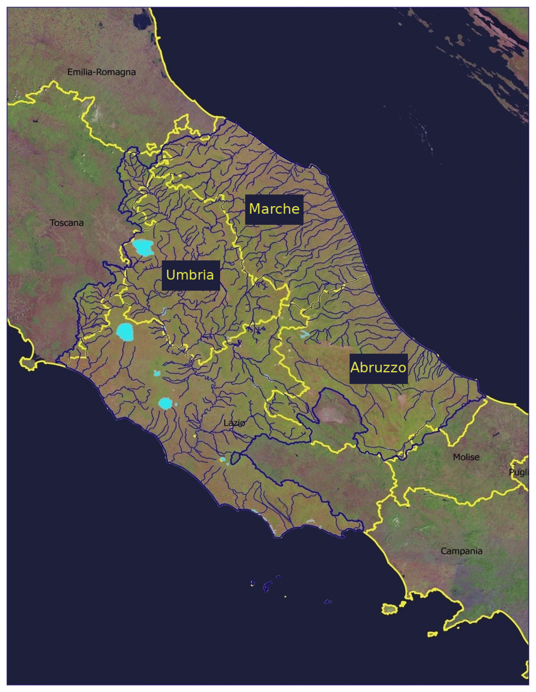
Figure 1 The Central Apennine Hydrological District (solid blue lines) and its main hydrography (thin blue lines). The north-eastern boundary is delimited by the Potenza river basin, while the south-eastern limit is represented by the Sangro basin in Abruzzo. The western side is delimited by the Tiber basin. Yellow lines indicate administrative boundaries of Italian regions. The three considered regions are highlighted: Umbria, Marche, Abruzzo (courtesy of the Tiber Basin Authority, https://www.autoritadistrettoac.it/i-numeri-del-distretto, last access: 10 June 2020).

The paper is organized as follows: a detailed description of the chosen hydrological model and of the proposed hydrological-stress indices is reported in Sect. 2, while a detailed description of the validation methods is provided in Sect. 3. In Sect. 4 the geographical framework of the study area is described, and in Sect. 5 the application of the proposed approach to several case studies is discussed.

2 Cetemps Hydrological Model

The Cetemps Hydrological Model (CHyM hereafter) has been developed at the Centre of Excellence CETEMPS, since 2002 (Verdecchia et al., 2008b; Coppola et al., 2007). The original purpose was the development of an operational hydrological model for flood alert mapping (Tomassetti et al., 2005). However, CHyM has also been applied in climatological studies to investigate the effects of climate changes on the hydrological cycle (Coppola et al., 2014; Sangelantoni et al., 2019).

CHyM is a fully distributed, physically based hydrological model, where the main hydrological processes are explicitly simulated by a physically based numerical scheme.

An important characteristic of the model is the possibility of simulating the hydrological cycle over any geographical domain with any spatial resolution up to the DEM resolution. To this aim, the NASA SRTM (Shuttle Radar Topography Mission) DEM source file (https://lpdaac.usgs.gov/products/srtmgl3v003/, last access: 4 April 2020) is implemented in the model with a native resolution of 90 m. Therefore, CHyM can simulate geographical domains with horizontal resolutions ≥90 m, even if the lower limit in choosing the spatial resolution deals with the validity of the numerical schemes used to simulate the hydrological processes (e.g. the kinematic wave of shallow water, which is used to solve the continuity equation, is considered a good approximation with a horizontal resolution of a few hundred metres).

For our national operational activity, we had divided the Italian territory into seven geographical sub-domains, each one characterized by a spatial resolution which is chosen in order to optimize computational requirements (lower resolutions mean faster simulations) and the correct drainage network extraction (higher resolutions mean more accurate drainage network reconstruction). In this paper, the operational spatial resolution associated with each sub-domain is the same as that of the operational set-up (Taraglio et al., 2019; Colaiuda et al., 2020). Starting from the NASA data, the DEM is upscaled by applying the cellular automata spatial interpolation technique (Coppola et al., 2007).

In this section, the surface runoff calculation scheme is described in detail; other parameterizations, such as evapotranspiration, infiltration, melting and return flow, are described in Coppola et al. (2014).

2.1 Runoff

To simulate the surface runoff, the continuity equation for surface routing and channel flow is explicitly solved. The flow direction for each grid point is established following the minimum energy principle; therefore, the flow direction is assigned to the grid point located adjacently to the maximum downhill slope. The channel flow is computed according to the kinematic-wave approximation of the shallow-water equation (Lighthill and Whitham, 1955), where the continuity equation is expressed through the following simplified form:

$$\begin{array}{}\text{(1)}& {\displaystyle \frac{\partial Q}{\partial x}}+{\displaystyle \frac{\partial F}{\partial t}}=q,\end{array}$$

where F is the flow cross-sectional area, Q is the flow rate of water discharge (m³/s), q is the rate of lateral water inflow per unit of length, t is the time and x is the coordinate along the river path.

According to the shallow-water approximation, the Saint-Venant equation for the momentum conservation is expressed through the rating curve approximation:

$$\begin{array}{}\text{(2)}& Q=\mathit{\alpha }{F}^m,\end{array}$$

where α is the kinematic-wave parameter and m is the kinematic-wave exponent, adimensional, which is assumed to be ≈1 for cylindrical river geometry. The kinematic-wave parameter α has the dimension of a speed:

$$\begin{array}{}\text{(3)}& \mathit{\alpha }={\displaystyle \frac{S^{\mathrm{1}/\mathrm{2}}{R}^{\mathrm{2}/\mathrm{3}}}{n\left(\mathit{\mu }\right)}},\end{array}$$

where S is the longitudinal bed slope of the flow element; n is Manning's roughness coefficient, depending on the land use type μ; and R is the hydraulic radius, considered a linear function of the drained area D, according to the following formula.

$$\begin{array}{}\text{(4)}& R=\mathit{\beta }+\mathit{\gamma }{D}^{\mathit{\delta }},\end{array}$$

where β, γ and δ are empirical constants to tune in the calibration phase. If the hydraulic radius is expressed in metres and the drained area is expressed in square kilometres, typical values of β, γ and δ are 0.0015, 0.35 and 0.33, respectively.

As for the surface flow outside the channel network, we assume that the surface water depth y is constant over each grid point; therefore, the continuity equation assumes the following form:

$$\begin{array}{}\text{(5)}& {\displaystyle \frac{\partial \mathit{\phi }}{\partial x}}+{\displaystyle \frac{\partial y}{\partial t}}=\mathit{\xi },\end{array}$$

where φ is flow rate over the longitudinal dimension (m²/s) of the grid point and ξ is the rate of water inflow per unit of area (m/s). The momentum equation has a linear relationship between the flow rate and the water depth, but Manning's roughness coefficient is increased by a factor M_n as the water is assumed to flow with a lower speed. For the operational simulations, the model default value of M_n for a river grid point is set to 4.5, but this parameter can be established during the calibration phase. An arbitrary drained-area threshold of 100 km² is set to distinguish the overland flow from the channel flow, which is expected to occur for drained areas wider than that threshold.

2.2 CHyM flood stress indices for operational activities

The hydrological model, CHyM, has been widely calibrated using climatological discharge time series of the river Po, as reported in Coppola et al. (2014). To this aim, it is important to note that the conditions of the Po are representative of many alluvial rivers in Europe (Di Baldassarre et al., 2009).

In general, long time series of flow discharge data are necessary to calibrate and validate hydrological models. However, such data are not always available from all Italian regions and, in many cases, rating curves used for the discharge estimation are not constantly updated. Furthermore, hydrometric-level measurements are not available or less available for major floods, when sensors installed along rivers stop working, due to severe meteorological conditions. For this reason, many data in the upper part of the rating curve are missed and larger errors in the discharge estimation are often associated with higher-discharge bins. Finally, hydrometers are installed over main river channels and small catchments are often excluded from discharge estimations, even if they are more prone to destructive flooding phenomena, especially in a complex-orography context. Hydrometric and/or discharge thresholds are defined punctually and differ for each sensor. In our stress index approach, discharge and runoff are combined with geographical information related to the upstream basin displacement, using other variables, such as the hydraulic radius (a linear function of the drained area) and time of concentration (that implicitly considers runoff conditions upstream). Therefore, stress indices are able to give information in each point of the drainage network, and their mutual variation from upstream to downstream along the river path is proportional. For this reason, general thresholds, valid for all grid points of the drainage network, may be defined. Moving from discharge-only to combined discharge-based and runoff-based indices, with the aim of calibrating such indices on a threshold basis for flood alert purposes, gives us the possibility of calibrating and validating different information, which is not the discharge amount but the river stress conditions, which is given by Civil Protection authorities using hydrometric thresholds, as well as stress timing. Furthermore, the good estimation of the stress state on a river channel is also provided by event reports and from press releases in those locations where no sensors are installed and, hence, no thresholds are defined. Since the index validation is not numerical, the problem of missing discharge data is overcome, the threshold-based calibration, rather than physical quantities, being a sufficient condition for our purpose to validate an alert system.

Moreover, it is important to highlight the influences of various flooding drivers (Ashley et al., 2005; Balmforth et al., 2006) since pluvial flooding happens together with fluvial flooding. Those flood scenarios were derived, for example, by adding rainstorms to the fluvial flood events, and this condition is easily found when we consider Italian river basins with a size of up to even a few tens of kilometres. In this case, fluvial and pluvial floods are combined and are sufficient from a few days to a few hours of intense rainfall, depending on the considered basin. For this reason, we developed two different indices linked to the different flooding sources: the CHyM Alert Index (CAI), a pluvial flood index related to the limited capacity of a drainage systems, and Best Discharge-based Drainage (BDD), a fluvial flood index related to deluges from river channels. These indices and the associated stress thresholds are general; the signal of the hydrological forecast is easy and quick to understand.

The hydrological-stress indices use the quantity of drained water and the geomorphological characteristics of the different basins. Although the units of measurement of the indices are expressed in millimetres, they do not represent rainfall. Both indices refer to the water accumulated on the ground over time. Three different thresholds for each of the two indices have been defined, in accordance with the protocols in use at the National Civil Protection Department. Since our intention is to develop unique thresholds with the same values at all grid points, we had to optimize threshold choice to maximize hit rate and minimize false alarms. In order to reasonably limit the scope of this paper, only results related to the moderate threshold (orange, pre-alert) are reported. The reason for our preference for this threshold lies in the consideration of its meaning in the Civil Protection alert system. In fact, the orange threshold exceedance can be considered the most crucial one for the Civil Protection Department, because its exceedance starts the activation of protection measures for people and infrastructure safety, as foreseen in risk plans. The indices have been tested over a wide area in Central Italy, where many different catchments are located. Index validation is presented in “perfect conditions”, i.e. forcing the hydrological model with observed meteorological variables. In our operational activity, as stressed in Ferretti et al. (2020) and Colaiuda et al. (2020), CHyM uses observed meteorological data for the spin-up process and meteorological model output to predict hydrological stress for the next 24/48 h. Therefore, the index stress map is released from 6 to 48 h in advance in the operational set-up.

2.2.1 CHyM Alert Index

The CHyM Alert Index (CAI) has long been used for the operational activities of flood alert mapping in Central Italy. The CAI is calculated as a function of the rainfall drained in each elementary cell of the simulated geographical domain. More specifically, the index is associated with each grid point, being the ratio between the total drained precipitation and total drained area in the upstream basin, with respect to the specific grid point. The proposed definition of the hydrological-stress index also has a simple physical interpretation: it represents the average precipitation drained in each cell, considering the rain falling over the whole upstream basin of the selected cell, during a time interval corresponding to the mean time of concentration. A first version of the CAI is described and tested in Tomassetti et al. (2005) and Verdecchia et al. (2008a); in its initial formulation, the mean time of concentration of the upstream basin was considered a fixed term (36 or 48 h, depending on the basin dimension). An updated version is presented in this work, where the average time of concentration, t_c, is explicitly calculated from each drainage path k, down to the considered grid point of coordinates i, j:

$$\begin{array}{}\text{(6)}& \stackrel{\mathrm{‾}}{t_{\mathrm{c}}^{i,j}}=\sum _{k=\mathrm{1}}^N{\displaystyle \frac{t_{k\to ij}^{i,j}}{N}},\end{array}$$

where N indicates the total possible flowing paths.

The time of concentration is computed for each grid point of the geographical domain. It can be defined as the time required for a raindrop to travel from the hydraulically most distant point in the watershed to the outlet. Each grid point is considered an outlet: namely, it may be a “mouth cell” draining toward a sea point, a “tributary mouth cell” draining toward the interception with the main river or a cell draining toward the border of the simulated domain. The water velocity for each cell of the domain is computed according to Eq. (3). The time of concentration used in the CAI calculation is an average calculated across all possible times of concentration resulting from draining paths toward the considered grid point.

The updated formula of the CAI is then the following:

$$\begin{array}{}\text{(7)}& \mathrm{CAI}={\displaystyle \frac{{\int }_{\mathrm{UP}}{\int }_{t-\mathrm{\Delta }t}^{t}P\left(t,s\right)\mathrm{d}t\mathrm{d}s}{{\int }_{\mathrm{UP}}\mathrm{d}s}},\end{array}$$

where P is the precipitation available for the runoff. The integral over the space s is calculated considering the whole upstream basin of the selected cell. For the stress state identification, three different thresholds have been defined, after carrying out empirical tests: each threshold has been adequately chosen to qualitatively match the three different Civil Protection states of hydrological criticality, as defined by the head of the Civil Protection Department (2016):

1. ordinary stress – 30 mm/d,

2. moderate stress – 60 mm/d,

3. high stress – 110 mm/d.

The definition of each hydrogeological criticality level (and related colour codes) is summarized in Table 1.

Table 1 Hydrogeological criticality levels officially defined by the Civil Protection authorities. Regional functional centres define hydrometric thresholds, in relevant river sections. Those thresholds are based on the return period concept, in order to individuate the criticality level to be assigned to the whole warning area (definitions conform to Deliberation no. 659/2017 of the Abruzzo Regional Council, Deliberation no. 148/2018 of the Marche Regional Council and Deliberation no. 2312/2007 of the Umbria Regional Council).

2.2.2 Best Discharge-Based Drainage index

The BDD index is linked to the CHyM-predicted discharge and is calculated, for each grid cell of the drainage network, according to the following formula:

$$\begin{array}{}\text{(8)}& \mathrm{BDD}\left(t\right)={\displaystyle \frac{Q\left(t\right)}{R^{\mathrm{2}}}},\end{array}$$

where Q is the discharge predicted at time t and R is the hydraulic radius of the selected elementary cell, calculated as a linear function of the upstream basin (see Eq. 4). BDD stress thresholds have been chosen following the same approach as that used for the CAI thresholds, in order to match the three relevant hydrological criticality levels:

1. ordinary stress – 3 mm/h,

2. moderate stress – 6 mm/h,

3. high stress – 11 mm/h.

3 Materials and methods

Floods are complex events, and data collection is not an easy task to achieve in this matter. The Italian government introduced the Cadastre of Events, in response to Directive 2000/60/CE, a registry where relevant hydro-meteorological events are listed and associated with a heterogeneous database of different territorial data, organized in geo-referred layers (e.g. flood time, localization and damage). Data sources are not necessarily objective measurements: collections may contain official Civil Protection reports and press releases, as well as other reports from local authorities. The official Hydrogeological Catastrophes GIS (geographic information system) archive is available online at http://sici.irpi.cnr.it (last access: 9 June 2020). However, the database updating was concluded in 2000: after this date, only a few Italian regions had moved to an alternative way of data collection, mainly represented by regional databases with different data structures and classifications, freely or restrictively accessible for external users. Considering the lack of official updated databases in the studied area, a huge but necessary effort was carried out to collect all available territorial data for the selected case studies, following the approach of the Cadastre of Events, in order to create our own database (ODB) with territorial, geo-referred information. Collected information in the ODB was used as reference data for the index validation process, discussed in the following section.

The ODB was filled by searching for and classifying the following heterogeneous data about the considered flood events:

• official Civil Protection event reports, issued by regional functional centres or environmental agencies;

• Copernicus Emergency Management Service;

• POLARIS database by CNR (National Research Council) IRPI (Research Institute for Geo-Hydrological Protection);

• data from the AVI project;

• press releases;

• photographic documentation from social media (e.g. YouTube, YouReporter), reporting major rainfall events, floods and landslides causing direct human consequences and damage in the investigated period;

• available hydrometric-level time series and thresholds, where updated (from the Dewetra Platform, Italian Civil Protection Department and CIMA Research Foundation, 2014).

The above-listed information was not all available for the same case study (CS); for this reason, a summary of the validation material found for each event is reported in Table 2. Moreover, to provide an overview of the data collection geographical distribution, the same information listed in Table 2 has been geo-referred and is shown in the maps of Figs. 2, 3 and 4. Besides the territorial information, other hydrological data were used for the validation process. The Italian ministerial decree (DPCM), issued on 27 February 2004 and concerning the “Operating concepts for functional management of national and regional alert system during flooding and landslide events for Civil Protection activities purposes”, establishes the regional functional centres to acquire and collect real-time data from monitoring networks. Hydrometric levels are identified as the quantities to be monitored in order to assign the critical level for, at least, moderate and high hydraulic risk to each warning area, through the definition of thresholds. Article 5 of the same decree defines that the real-time validation of prediction systems is made through the monitoring of moderate and high hydrometric-level threshold exceedances, for the main river channels. Secondary drainage networks with drained areas of less than 400 km² are not included in this kind of validation.

Table 2 Summary of relevant damage reported for each case study and information sources used.

OR: official Civil Protection report; PR: press releases; V: videos.

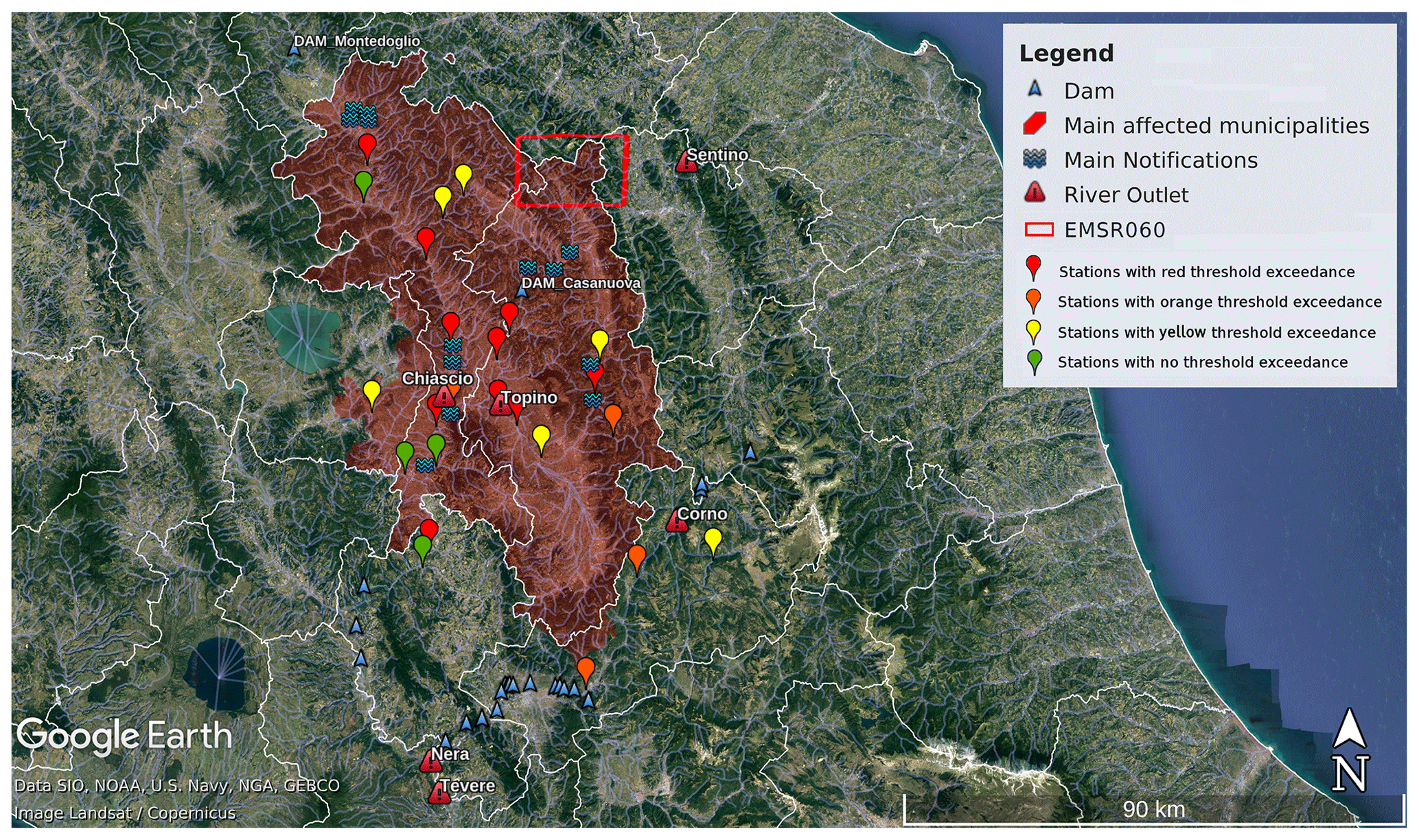
Figure 2 Geo-referred information of the ODB for CS01, Umbria region, with localization of main recorded floods (blue waves), hydrometric stations used for the indices' validation (pinpoints). Red triangles indicate the position of outlets of the main rivers involved, while blue triangles indicate the presence of dams. Hydrometric station pinpoints are coloured according to the maximum hydrometric threshold reached during the event. Municipality areas affected by flooding are filled in red. The red rectangle represents the involved area published on the Copernicus Emergency Management Service platform (https://emergency.copernicus.eu/mapping/list-of-components/EMSR060, last access: 9 June 2020). © Google Earth.

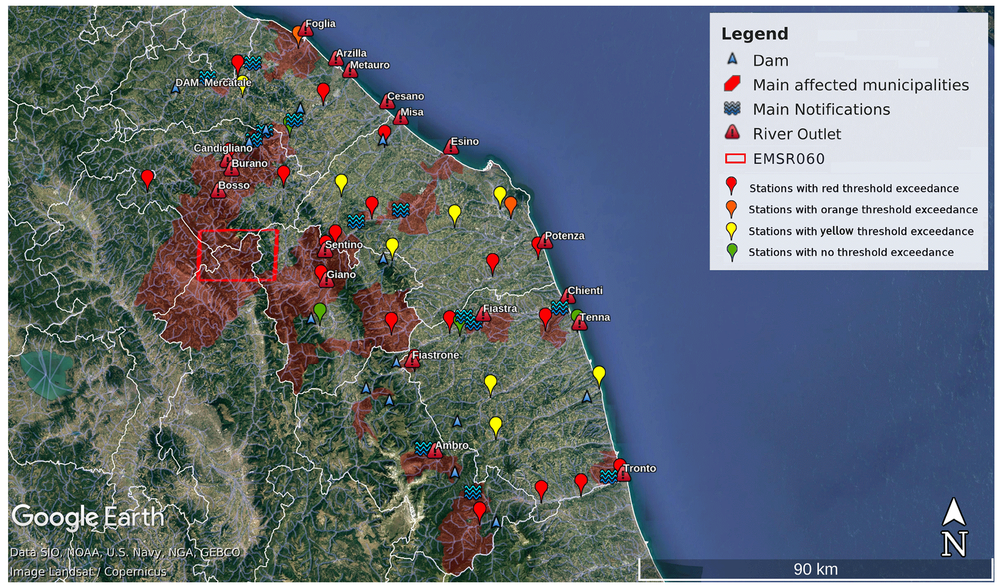
Figure 3 Geo-referred information of the ODB for CS02, Marche region, with localization of main recorded floods (blue waves), hydrometric stations used for the indices' validation (pinpoints). Red triangles indicate the position of outlets of the main rivers involved, while blue triangles indicate the presence of dams. Hydrometric station pinpoints are coloured according to the maximum hydrometric threshold reached during the event. Municipality areas affected by flooding are filled in red. © Google Earth.

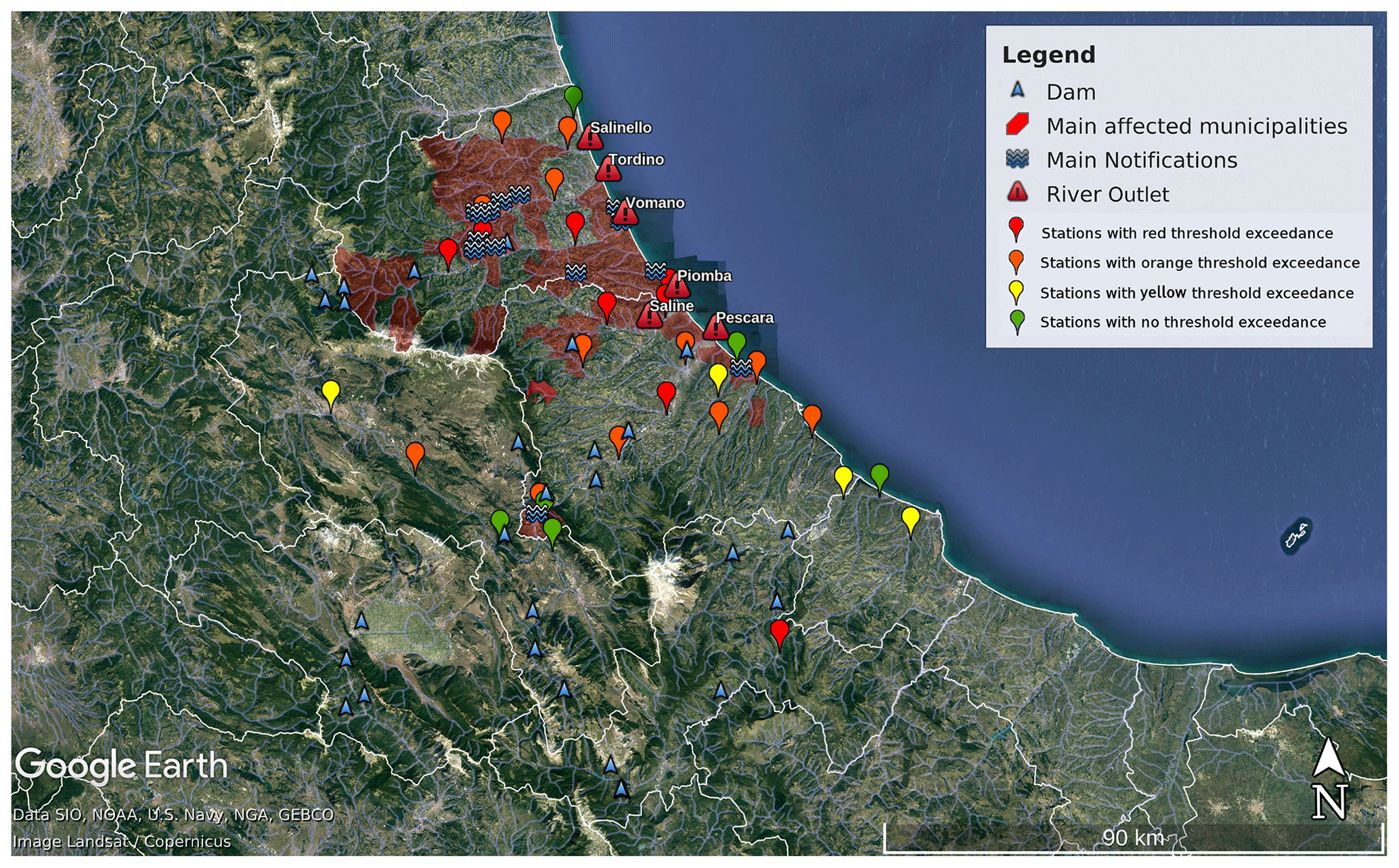
Figure 4 Geo-referred information of the ODB for CS03, Abruzzo region, with localization of main recorded floods (blue waves), hydrometric stations used for the indices' validation (pinpoints). Red triangles indicate the position of outlets of the main rivers involved, while blue triangles indicate the presence of dams. Hydrometric station pinpoints are coloured according to the maximum hydrometric threshold reached during the event. Municipality areas affected by flooding are filled in red. © Google Earth.

The definition of water level critical thresholds (Italian Law No. 59/2004; Fassi et al., 2008) is carried out for each Italian region by local Civil Protection authorities (regional functional centres) at the station level (Fassi et al., 2008; Brandolini et al., 2012; Mysiak et al., 2013). A colour code is then assigned to each hydrometric threshold (see details in Table 1), indicating four different alarm levels, corresponding to specific hydraulic risk management actions, activated at an institutional level (Italian Legislative Decree No. 01/2018). However, as recognized by the Italian Institute for Environmental Protection and Research (ISPRA), the hydrometric level is a strongly non-stationary variable, as it is influenced by riverbed erosion and deposition processes (Braca et al., 2013). The hydrometric zero needs to be recalibrated, establishing an updating frequency adequate for the river flow regime and local hydrogeological factors. Moreover, the calibration should be carried out after flood occurrences, when the riverbed shape is significantly modified. Then, the hydrometric thresholds need to be revised correspondingly. After the application of Italian Law No. 183/1989, the management of the gauge's network and data collection is devolved to the regional authorities. Even though a territorial approach is useful for a rapid response to risk scenarios, competency fragmentation among different entities has caused inhomogeneities in hydro-meteorological data availability and quality (e.g. rating curve updates, historical hydro-meteorological data time series, hydrometric threshold availability for all stations) with significant differences among the 20 Italian regions.

For all the aforementioned reasons, a deterministic hydrological flood prediction validation over a wide, interregional area can be challenging or not universally applicable, due to missing or obsolete information. Moreover, the discharge computation in hydrological models is affected by systematic biases when the hydrological network is exploited for hydropower production, irrigation, or industrial and domestic usage; in most cases, data about water uptake are scanty or incomplete, as they are collected by a variety of public and private actors and difficult to obtain. Another common issue for the spatial validation relates to threshold inference in ungauged areas. Alfieri et al. (2017) highlighted that floods and flash floods usually occur in ungauged catchments; for those situations, post-event survey reports represent the only source of information. Besides, even if present, gauge data may be unavailable during a severe event or damaged by the flood.

The hydrological-stress index validation was first assessed through a qualitative approach, by selecting the strongest recorded signal of upcoming severe events from the hydrometric-level time series and verifying the actual occurrence of floods in the areas where they were forecasted. To this aim, hydrological-stress index maps are compared with ODB geo-referred maps. In addition, an objective analysis is carried out by applying both statistical dichotomous and continuous scores.

3.1 Statistical dichotomous analysis

Primarily, the index grid map was spatially co-located with the hydrometers' position by choosing the nearest grid point to the station geographical coordinates after verifying the correspondence between the grid point upstream drained area calculated by CHyM, with the real value declared in the official station registry (where available).

As for the time co-location, both water level and indices' time series are hourly, and it might appear straightforward to investigate the potential threshold exceedances by comparing the same time step. However, during a flood wave, it is not infrequent to have water level data corrupted by measurement errors during the flood wave transition (i.e. a solid surface stationing for a certain period under the hydrometric sensor). For this reason, the time location is carried out by associating a mobile interval of 3 h (the target time step ±1) of observations to each index time step. The choice of this confidence interval is arbitrary, although it is based on the authors' experience. The contingency table was then built, for each station point and for each index, considering the match between the co-located moderate hydrometric threshold exceedances (THR 2 in Table 1) and the moderate index threshold exceedances. Differently from water level thresholds, CAI and BDD index thresholds have the same value for all the grid points of the drainage network. These numerical thresholds are 6 mm/h for BDD and 60 mm/d for CAI, respectively; the choice of these values is justified a posteriori considering the performances of the proposed indices for different severe events analysed, during 10 years of operational activity (Colaiuda et al., 2020). Under the most natural conditions and with continuous updating of the hydrometric thresholds depending on the morphodynamic variability in the basin, the proposed threshold levels for BDD and CAI should appear very close to the water level threshold for the specific site.

The dichotomous scores include the accuracy (A), the probability of detection (POD), the false alarm ratio (FAR). To build such a table, a flood event is considered an observed yes/no event if the water level exceeds/does not exceed the empirical threshold; a flood event is an estimated yes/no event if the estimated index exceeds/does not exceed the BDD and CAI thresholds (Table 3). The A, POD and FAR scores are defined as follows:

$$\begin{array}{}\text{(9)}& {\displaystyle }A={\displaystyle \frac{H+\mathrm{CN}}{H+Mi+\mathrm{FA}+\mathrm{CN}}},\text{(10)}& {\displaystyle }\mathrm{POD}={\displaystyle \frac{H}{H+Mi}},\end{array}$$

$$\begin{array}{}\text{(11)}& \mathrm{FAR}={\displaystyle \frac{\mathrm{FA}}{H+\mathrm{FA}}}.\end{array}$$

The calibration of the indices' thresholds was chosen to maximize the hit rate H, though at the cost of a higher average false alarm rate: choosing a lower threshold increases detection skills of events with high uncertainty, according to Alfieri et al. (2017). All listed scores range from 0 to 1, where 1 is the optimal value for A and the POD, while 0 indicates the best possible score for the FAR.

Table 3 Contingency table structure used for the validation analysis.

3.2 Catch rate

The catch rate (CR) was estimated for each index, to investigate effectiveness in detecting or missing correct flood warnings. To this aim, the orange (moderate) hydrometric-level threshold exceedances (THR2s) were chosen as a term of comparison with the corresponding moderate CAI and BDD index thresholds. A match occurs when the hydrometric THR2 is exceeded and the moderate index threshold is exceeded or when the hydrometric THR2 is not exceeded and the moderate index threshold is not exceeded, within a 24 h time range. A Boolean value $\mathrm{0}/\mathrm{1}$ is then assigned when a match occurs. CR is calculated as the ratio between the number of correct matches found and the total number of analysed stations N:

$$\begin{array}{}\text{(12)}& \mathrm{CR}={\sum }_{i=\mathrm{1}}^N{\displaystyle \frac{\mathrm{1}}{N}}{\mathrm{CESA}}_i.\end{array}$$

Here the abbreviation CESA stands for correct estimated state of alert for the i sensor, which assumes a value of 1 when estimation matches observation and a value of 0 when that match does not occur.

3.3 Time peak analysis

In order to further evaluate the timing accuracy of the BDD index and CAI, all the available observed water level time series were compared to the indices' time series. Because of the comparison between two different physical quantities, the chosen statistical scores are typically used for signal studies. The first statistical analysis was made through the calculation of the lag time peak (LTP), to investigate the simultaneity of occurrence between the water level peak and the indices peak. According to the Italian ministerial directive concerning “Operational guidelines for emergency management”, issued on 3 December 2008, a lag time of “a few hours” (less than 12 h) is estimated to be between an event occurrence and the activation of the Civil Protection coordination unit. In light of the above, we established that an adequate lag time peak for flood prediction should not exceed 3 h. According to other authors (see, as an example, Rabuffetti et al., 2008), the relative lag time peak (RLTP), defined as the ratio between the LTP and the average time of concentration of the upstream basin, can be calculated.

3.4 Correlation time delay (CTD)

The cross correlation (CC) is typically used in signal theory (Rabiner and Gold, 1975; Rabiner and Schafer, 1978; Benesty et al., 2004), for the assessment of similarity between two signals. Given two discrete series x(t) and y(t), each one of N components, the cross correlation is calculated as the dot product of the series:

$$\begin{array}{}\text{(13)}& \mathrm{CC}={\sum }_{i=\mathrm{1}}^{N}x\left(t_i\right)y\left(t_i\right).\end{array}$$

The same product can be calculated, shifting the two signals of a time lag L:

$$\begin{array}{}\text{(14)}& \mathrm{CC}\left(L\right)={\sum }_{i=\mathrm{1}}^{N}x\left(t_i\right)y\left(t_i+L\right).\end{array}$$

The correlation time delay (CTD) is then defined as the value of time lag L that maximizes the previous product.

$$\begin{array}{}\text{(15)}& \mathrm{CTD}=\mathrm{CC}\left(L\right)\end{array}$$

CTD represents an estimation of time shift between two series; therefore, we found this score to be suitable to measure the effectiveness of the signal given by the hydrological-stress indices.

3.5 Derivate dynamic time-warping analysis

Dynamic time warping (DTW; Berndt and Clifford, 1994; Keogh and Ratanamahatana, 2005; Maier-Gerber et al., 2019; Di Muzio et al., 2019) allows us to stress (or compress) two time series to achieve a reasonable fit between them. The idea of the method is that the similarity between two sequences can be estimated by “warping” the time axis of one (or both) sequences, to achieve a better alignment. Although DTW has been successfully used in many domains, it may lead to obtaining incorrect results; as an example, the technique may fail in finding the optimal alignment because a feature (i.e. peak or local minimum) in one sequence is higher or lower than its corresponding feature in the other sequence.

To overcome this problem, Keogh and Pazzani (2001) proposed the computation of warping using the local derivative of the time series to be compared and called this algorithm Derivative Dynamic Time Warping (DDTW).

The numerical procedure for the DTW calculation can be summarized as follows: given two discrete series x(i) and y(j) of N and M components, respectively, an N-by-M matrix is built. An element V(i,j) contains the Euclidean distance between the ith element of the first sequence and jth element of the second sequence. For this matrix, a warping path W is defined as a contiguous set of L matrix elements, and the measure of misalignment d for the path W is given by

$$\begin{array}{}\text{(16)}& d\left(W\right)={\displaystyle \frac{{\sum }_{i,j}V\left(i,j\right)}{\frac{\mathrm{1}}{\mathrm{2}}L\left(L-\mathrm{1}\right)}},\end{array}$$

where the sum in the numerator is carried out over all the elements belonging to the warping path W. The denominator is used to normalize different length sequences. The DTW index is then calculated as the minimum value of d(W), considering all the possible paths W.

$$\begin{array}{}\text{(17)}& \mathrm{DTW}=d\left(W\right)\end{array}$$

For instance, if the two considered sequences are aligned and have the same number of components (N=M), the optimal path will be the N diagonal elements of matrix V.

The DDTW (Fig. 5) algorithm implementation replaces the data time series with their first derivative and the Euclidean distance is measured on them. The first derivative has been calculated for each time series as follows:

$$\begin{array}{}\text{(18)}& D\left(x\left[i\right]\right)={\displaystyle \frac{\left(x\left[i\right]-x\left[i-\mathrm{1}\right]\right)+\left(\right(x\left[i+\mathrm{1}\right]-x\left[i-\mathrm{1}\right])/\mathrm{2}}{\mathrm{2}}}.\end{array}$$

Figure 5 Graphical representation of DDTW correspondences between two first derivatives of time series x(t) and y(t). In this case, time series are represented by two generic profiles of the hydrometric water level and the BDD index, at the same station point (from Keogh and Pazzani, 2001).

4 Study area description

The study area covers the Central Apennine District (Fig. 1), with an extension of 42 506 km² and about 8 million inhabitants. The northern part, which includes the upstream basin of the Tiber from the confluence with the river Nera, is characterized by a less dense draining network with respect to the lower part of the basin. This area has complex hydrography, characterized by both perennial rivers, constantly fed by groundwater, and seasonal streams, which are activated only in rainy periods. Moreover, plenty of artificial reservoirs and hilly ponds take up surface runoff water. The Adriatic slope is located over the central part of the district, extending from the upper Marche region (the river Potenza) to the southern part of the Abruzzo region (river Sangro). The lower path of the Tiber is also part of this area, together with the tributaries on the left bank, from the Nera to Aniene rivers.

This area is affected by inundations along major rivers, as well as flash floods in torrents and minor streams, especially on the heels of the ridge, where high-intensity rainstorms cause lowland flooding. Most of the drainage network is characterized by significant water storage (with a quite constant spring flow rate during the year) and marked by hydroelectric power plants, built since the last century (Tiber Basin Authority, 2010). The peak discharge variation depends on the storage type: generally, the effect of a reservoir on flood control results from a combination of regulated and unregulated storage (Volpi et al., 2018). The former, used in the analysed area, is less efficient in flood-peak reduction than regulated storage, as it begins filling even before it is needed. Moreover, the effect of a flood control reservoir depends on the combination of off-stream or on-stream detention ponds as reported by Ravazzani et al. (2014). Dams and reservoirs play an important role during flood events (Rodda, 2011; Kundzewicz et al., 2014; Ayalew et al., 2017; Habets et al., 2018): this role is not always favourable; they adversely affect the extent of an inundation due to dike breaches, blockage of bridges and culverts by debris. Anyway, weak coordination between different actors involved in water resource management may significantly affect flood dynamics. In multi-purpose reservoirs, competing interests represent a key issue in flood regulation: irrigation, hydropower generation and flood control generally compete, even when the reservoir is owned by a single country or agency. This conflict of interests is heightened when the basin is interregional, as in the case of the Central Apennine District. For those reasons, the WMO (2009) recommends carefully evaluating the flood timing and dynamics.

5 Results and discussion

In this section, the analysis of a meteo-hydrological event that occurred in Central Italy on 11–13 November 2013 is proposed. The 3 d event was characterized by intense precipitation, involving the whole Central Apennine ridge and three different regions, progressively affecting the Adriatic side of the central part of Italy, moving from north to south. To better organize our analysis, the event was divided into three different case studies, related to three different regions involved: Umbria (CS01), Marche (CS02) and Abruzzo (CS03). The CHyM simulations were set to three different geographical domains, as shown in Fig. 6. The event was very intense and caused much damage and a few fatalities in all regions; an overview of the phenomenon is reported in Table 2, where relevant information about observed effects and sources of information are provided. Details of links pointing to each source used to organize the ODB are provided in the Supplement, where all hit municipalities and affected rivers are also listed.

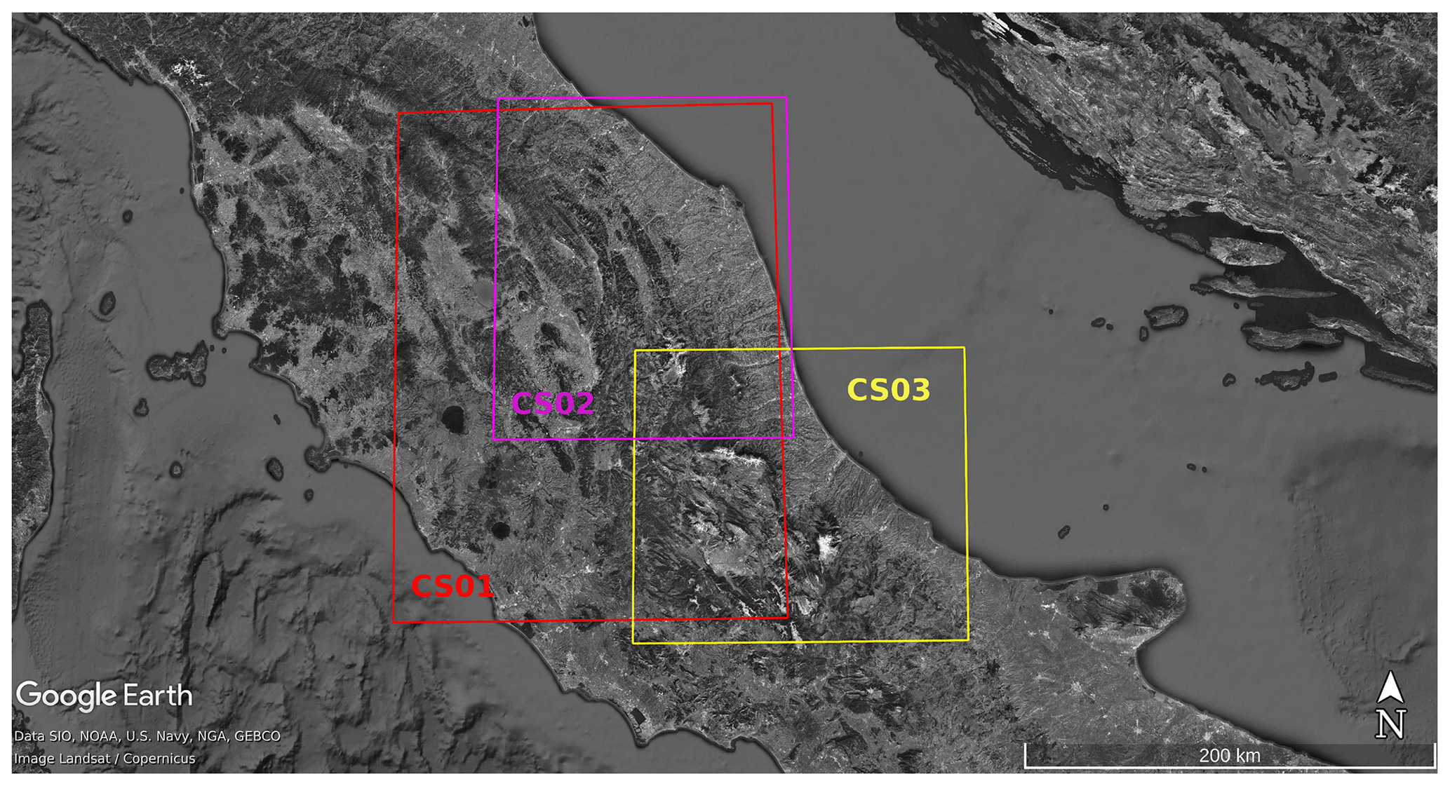
Figure 6 Three CHyM geographical domains used for the simulation of the corresponding CSs. The red square encloses the Umbria region and the rest of Tiber basin for CS01; the pink square refers to CS02 (Marche region), and the yellow square encompasses the Abruzzo region for CS03. © Google Earth.

5.1 Synoptic analysis

On 11 November 2013, a large synoptic-scale meteorological system originated from the Atlantic Ocean and moved into the Mediterranean area. In particular, the cold air coming in from southern France has induced rapid cyclogenesis on the Gulf of Genoa. The barometric minimum moved southward along the Italian Peninsula and reached the Tyrrhenian Sea on 12 November. The persistence of the occluded front over Italy caused heavy and long precipitation, initially affecting northern regions and, progressively, central and southern areas, as the minimum moved toward the Libyan coast, on 13 November. The precipitation was widespread, with a huge amount. According to the event reports from regional Civil Protection authorities, registered precipitation amounts were almost 300 mm/72 h in several areas, mainly located along the Apennine ridge, between the Marche and Umbria regions (Fig. 7).

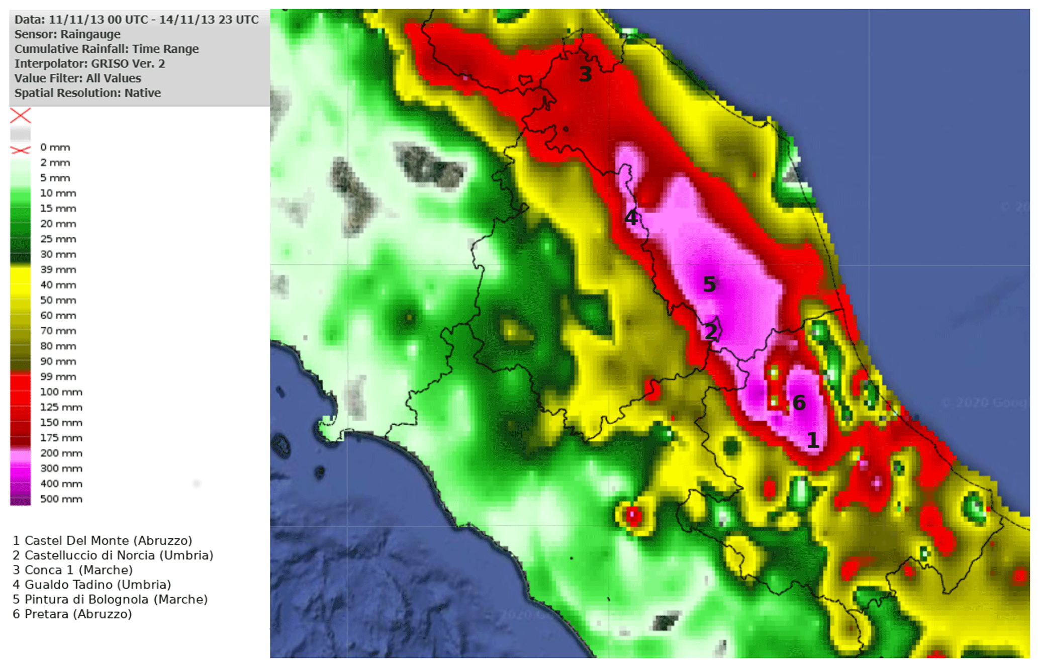
Figure 7 Total accumulated rainfall (spatialization from rain gauge official network) during the event, from 11 November 2012 00:00 UTC to 13 November 2013 23:00 UTC (picture generated from the Dewetra Platform, Italian Civil Protection Department and CIMA Research Foundation, 2014). The localization of the six rain gauges are indicated on the map: (1) Castel del Monte station (Abruzzo region), (2) Castelluccio di Norcia station (Umbria region), (3) Conca 1 station (Marche region), (4) Gualdo Tadino station (Umbria region), (5) Pintura di Bolognola station (Marche region), (6) Pretara station (Abruzzo region). The rain gauges recorded significant accumulated rain (up to 400 mm/72 h, purple area).

5.2 Case study analysis

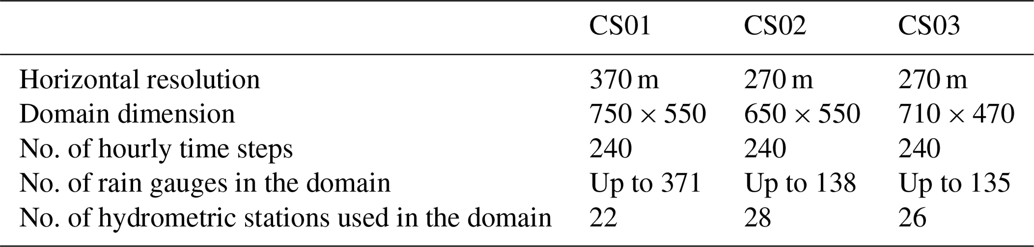
Hydrological simulations were carried out over a geographical domain larger than the areas where floods were actually observed, in order to verify the absence of predicted hydrological-stress conditions in those areas where the hydrological criticality level has not been exceeded. Hydrological simulation was set by using a spin-up time of 120 h for all case studies, before the day of the hydrological event. Given the small extension of the involved catchments, 120 h of spin-up seems to be enough for the model initialization. It should be noticed that stress indices are used to detect hydrological situations where relevant discharges, driven by significant rainfall events in a short time (a few hours to a few days) are present. The selected case studies affected different regions of Central Italy characterized by catchments of different sizes and geomorphological characteristics, allowing the evaluation of index feasibility in heterogeneous domains. Spatial and temporal characteristics of the hydrological simulations are reported in Table 4.

Table 4 CHyM domain set-up for the analysed case studies. Please note that the rain gauge data may not all be available during the entire event, due to interruption of electric supply.

As discussed in Sect. 3, the ODB information about case studies was geo-referenced on a Google Earth maps (Figs. 2, 3, 4). The blue wave symbols indicate reported inundations, and the pinpoints show the hydrometers displacement; the colour assigned to each pinpoint highlights the observed state of alert, namely, the hydrometric threshold exceedances (see Table 1 for further details). On the same maps, the drainage network is represented by blue lines; white lines indicate alert zone boundaries, defined by the Civil Protection, reddish areas encompass the administrative boundaries of the main affected municipalities (i.e. where a flood was reported), while the small blue triangles highlight the main water reservoirs located inside the domain. In Figs. 2 and 3, red rectangles represent the flood-affected area published on Copernicus Emergency Management Service platform (EMS Rapid Mapping activations (EMSR060), https://emergency.copernicus.eu/mapping/list-of-components/EMSR060, last access: 9 June 2020).

5.2.1 Case study 1 – Umbria region

From 11 to 12 November 2013, a severe weather event hit the Umbria region. The event was mainly concentrated over the north-eastern part of the region, along the administrative boundary with the Marche region. According to the data provided by the official hydro-meteorological monitoring network, precipitation was persistent and intense, resulting in exceptional amounts, up to 440 mm in the Castelluccio di Norcia station and 330 mm in Gualdo Tadino in 72 h (see Fig. 7). Flooding affected main rivers, as well as small catchments (river outlet highlighted in Fig. 2), such as the Tiber, the upper Chiascio, and the Topino basins. In particular, the flooding on the river Sentino, flowing along the boundary with the Marche region, caused damage to 12 residential buildings and temporarily isolated the Branca hospital, due to considerable road and bridge disruption. All municipalities of the Apennine ridge registered damage. A flood wave occurred over the Nera and the Corno tributary. According to the Civil Protection official report, Montedoglio and Corbara dams played a crucial role in the flood wave lamination and phase shifting in the Tiber and Casanuova dam did the same in the Chiascio (Fig. 2, blue triangles). The initial value of water in the two reservoirs is not considered, because no data are provided about release and withdrawals of water from the water reservoirs. Due to the lack of water storage data, it is not possible to properly assess the flow discharge simulation; therefore, we can only state that the discharge simulation from our model differs from observations and highlight the presence of an anthropic impact due to artificial water reservoirs displaced upstream. According to our experience, we have found that indices' peak timing and their shifts with respect to the observed hydrometric level can provide information about the flood management through water reservoir release and withdrawals, which are able to postpone (or anticipate) discharge maxima's propagation downstream.

For this first case study (CS01, Fig. 6), the main characteristics of hydrological simulation are reported in Table 4. The hydrological model has been forced with observed precipitation data from almost 370 rain gauges, located in the geographical domain. The CAI and BDD index maps obtained for CS01 are shown in Fig. 8. Hydrological-stress indices are computed at hourly time steps. However, the map refers to a 24 h time interval, where the maximum daily value of the index is assigned to each grid point. In other words, the map gives an idea of the maximum stress conditions that may occur across the whole day. Moreover, the actual drainage network is denser in the highlighted catchments; however, we decided to plot only grid points with a drained area larger than 15 km², to improve the map visualization and interpretation.

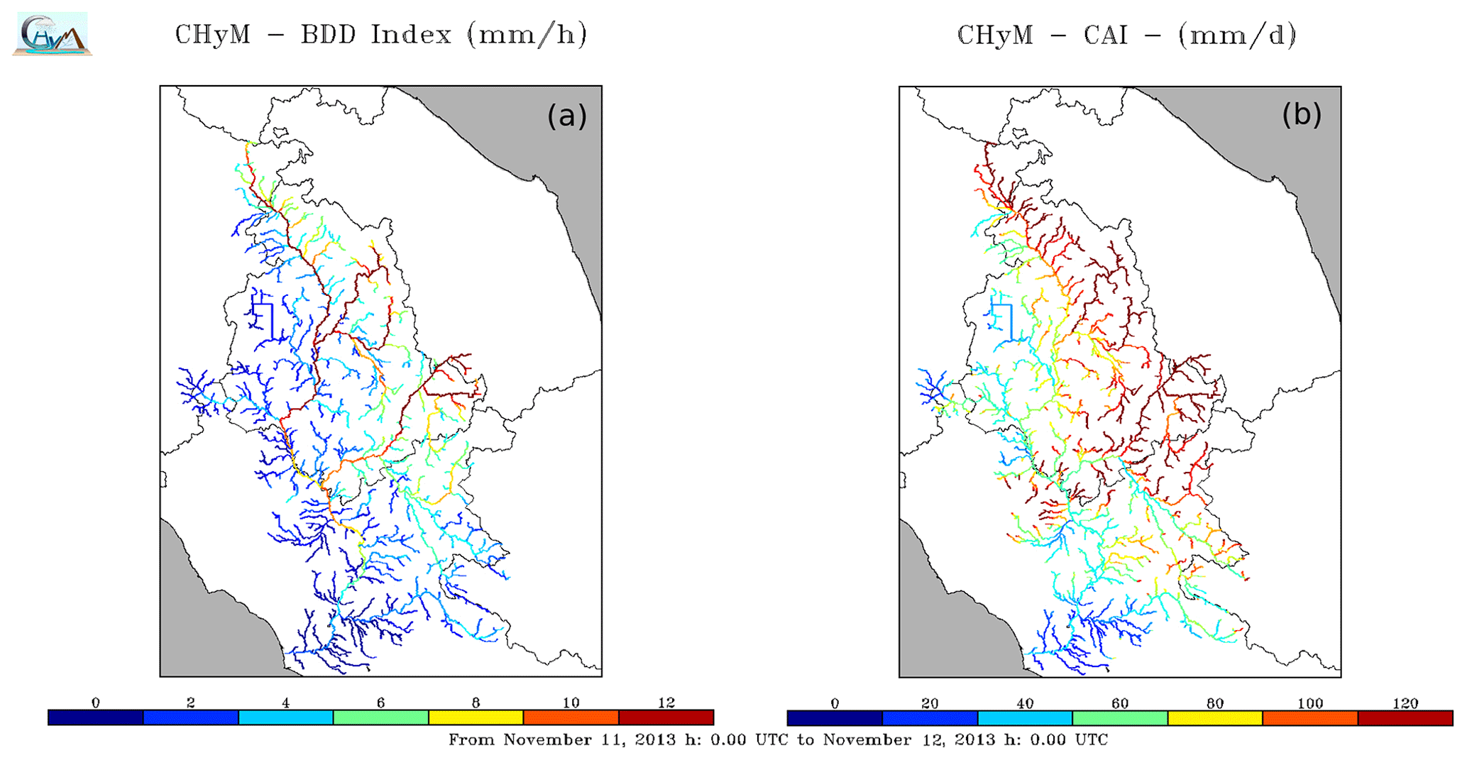
Figure 8 CS01 24 h maps of the BDD index (a) and the CAI (b) obtained for 11 November 2013, by forcing CHyM with observed rainfall data. Warmer colours indicate river segments with higher flood stress. In both figures, the Umbria region drainage network, as well as the whole Tiber basin, is highlighted.

A qualitative comparison of Figs. 2 and 8 allows us to identify similarities in the hydrological-stress spatial distribution and observed inundations. The higher CAI and BDD stress degree is mainly given on the north-eastern side of drainage network, from the upper Umbria regional boundary and along the slope exposed to the Adriatic side. All the reported damage and orange/red hydrometric levels are observed in the same area. The western side of Umbria was not significantly affected by the event, and no relevant stress degree is given by indices.

The CAI overestimates the hydrological-stress extension in the south-eastern part of the region, near the boundary with the Lazio region. Moreover, a difference between the two indices needs to be highlighted: the BDD index stress degree is lower in the minor drainage network and relevant in the main river channel. This effect is due to the different nature of the indices and the different physical quantities considered in their calculation: the CAI is directly linked to the precipitation rate, resulting in higher responsiveness in the smallest river channels, where the high-peak precipitation-driven flood is the predominant mechanism for inundations. On the other hand, the BDD index calculation is based on the discharge value and responsive to runoff-driven floods, resulting from the combination of different hydrological processes, such as rainfall runoff, infiltration, soil moisture and melting.

Besides the spatial assessment, timing analysis is given through a heterogeneous comparison between hydrometric-level time series and indices' time series (Fig. 9), for six relevant hydrometric stations located in the upper part of the Umbria region, where the orange hydrometric threshold was exceeded. The represented quantities, as well as the associated thresholds, are normalized. Indices' increasing and decreasing rates show a similar behaviour with the hydrometric-level trend, and maximum occurrence is concomitant in the Tiber and Topino river stations and slightly anticipated (from 3 to 6 h) by the indices in the Chiascio and Nera rivers.

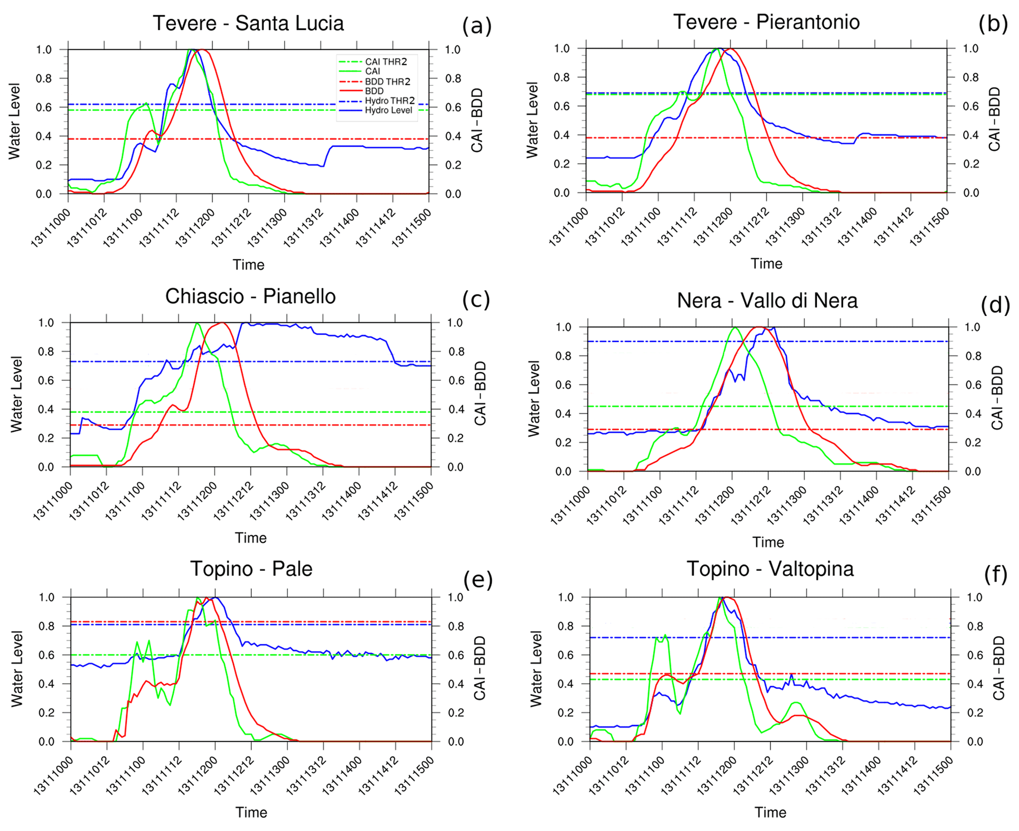
Figure 9 Time series comparison for six hydrometric stations: BDD hourly profile (red line), BDD moderate threshold (flat red line), CAI hourly profile (green line), CAI moderate threshold (flat green line), hydrometric-level hourly profile (blue line) and hydrometric-level moderate threshold (flat blue line). Quantity profiles and related thresholds are normalized.

As stated at the beginning of this paragraph, artificial water storage and lamination played an important role in the flood wave management in this area. Flood abatement is achieved by detaining and later releasing a portion of the peak flood flow (WMO, 2009), and different kinds of reservoirs have been found to cause different release dynamics.

Focusing our analysis on the Pianello station (Fig. 9d), downstream of the Casanuova dam, the index peak shifting may be due to the lamination of flood waves by the on-stream water storage system. The presence of the Montedoglio dam, upstream of the Tevere–Santa Lucia and Tevere–Pierantonio stations (Fig. 9a and b), does not produce the same effect and peak timing appears to be concomitant with the hydrometric-level peak. Although the dam has retained almost all of the inflows from the upstream basin (up to 13 November at 12:00 UTC), its off-stream position, rather than the timing, allowed the regulation of the intensity of the flood (Fig. 9a, b). The increasing hydrometric profile after 13 November 2013, 12:00 UTC, indicates the artificial release after the end of the event.

Despite the presence of large and small detection storage affecting the indices' accuracy, the average CR value, calculated over 22 hydrometric stations is 0.86 for BDD and 0.77 for the CAI. This result supports the qualitative analysis discussion, where a spatial correspondence between the index map and the ODB map was observed.

Threshold exceedance hourly matches have been calculated over the same 22 hydrometric stations, belonging to seven different catchments, for a total amount of 2574 h analysed (120 h per station); resulting scores are summarized in Table 5 (score breakdowns for each station are not shown). The accuracy of the prediction is above 0.8 for both indices, while the POD is around 0.7 for BDD and 0.5 for the CAI. The false alarm rate is around 0.45 in both cases; however, when the flood dynamics are artificially regulated, the misalignment between observed and simulated peaks, analysed in discussion of Fig. 9, leads to increasing values of the FAR. The index stress overestimation may be attributable to missing territorial information; however, without evidence of this, we can only assess that the model did not properly simulate hydrological stress.

Table 5 CAI and BDD index scores for all CSs. Values for single CSs are averages calculated over all hydrometric stations located in the domain.

As for the timing analysis, the resulting LTP is <1 h for BDD and about −7 h for the CAI. In general, all timing scores resulted in being better for BDD than the CAI, with a slight tendency to anticipate the peak values.

5.2.2 Case study 2 – Marche region

The official report of the Marche Region Civil Protection described the occurrence of hydrological criticality over the whole region, especially in the inner areas, along the Apennine ridge, where maxima of rainfall were registered. Precipitation peaks were up to 487 mm in 72 h in the Pintura di Bolognola rain gauge (south-east of the region) and 200 mm in Conca 1 (north-east of the region) (Fig. 7). Floods affected many rivers in the upper Marche: a critical situation over the Metauro basin was recorded over the upstream tributaries (the Candigliano, Bosso and Burano). Other floods were also recorded in the Cesano, Misa and Arzilla basins, as well as in the river Chienti, where a flood wave propagated, starting from the Fiastrone and Fiastra upper tributaries. In the Foglia basin, the Mercatale dam laminated part of the flood from the early hours of 11 November until the afternoon, when its maximum accumulation capacity was reached. The upper parts of the Potenza, Tenna and Tronto basins were also affected by floods.

A qualitative analysis of the hydrological-stress spatial distribution by comparing ODB data (Fig. 3) and index maps (Fig. 10) was carried out, to identify a geographical match between recorded inundations and simulated hydrological stress.

Figure 10 CS02 24 h maps of the BDD index (a) and the CAI (b) obtained for 11 November 2013, by forcing CHyM with observed rainfall data. Warmer colours indicate river segments with higher flood stress. In both figures, the Marche region drainage network is highlighted.

For this case study (CS02, Fig. 6), the main characteristics of hydrological simulation are summarized in Table 4.

The hydrological model has been forced with almost 138 rain gauge data, used to rebuild the precipitation field. The main affected municipalities lay on the piedmont areas of the Apennine ridge (the lower part of Fig. 3), where maxima of precipitation were registered. However, the flood wave originating from those areas propagated downhill, toward the Adriatic Sea, affecting all the river systems, where damage and inundations occurred and hydrological-level criticality thresholds were exceeded. The CAI map (Fig. 10b) has identified almost each grid point of the drainage network with the highest stress degree, while in the BDD map maximum stress over the main rivers (Fig. 10a) is highlighted. The difference between the behaviour of the two indices is due to the same mechanism described for CS01.

In the Marche region, many dams affect the natural river flow. The normalized indices and hydrometric-level profiles are shown in Fig. 11: the effect of Mercatale dam lamination caused a progressively larger hydrometric peak shifting along the river Foglia (Fig. 11c and d). The precipitation resulted in high supplies to the reservoirs of the Metauro, Chienti and Tronto basins where it was necessary to retain part of the inlet flow during the event. Where the storage capacity allowed us to manage the amount of precipitated rain, a rolling service was carried out. Maximum peak shifting is shown in Fig. 11f, for the Fiastrone station. A first hydrometric peak is slightly postponed by indices, while a same-magnitude secondary peak is weakly detected. A relevant impact on the Fiastrone station is determined by the presence of unregulated on-stream storage from Lake Fiastra, which is the largest hydroelectric basin in the Marche region. The other time series shown in Fig. 11 are characterized by a synchronous peak of indices and the hydrometric level. Dichotomous and continuous analysis scores for CS02 are shown in Table 5: for this case study, 28 stations' time series have been analysed, covering 13 different basins. In this case, an accuracy of 0.8 is reported for both indices, with the POD being around 0.70 for BDD and 0.55 for the CAI. A FAR score of 0.37 for BDD and 0.43 for the CAI has been calculated. The LTP is less than 1 h for BDD and −4 h for CAI, resulting in an RLTP of 0.05 for BDD and −0.56 for the CAI. The CTD is significantly lower in BDD with respect to the CAI, with values of −1.4 and −5.6, respectively. The DDTW is 0.04 for BDD and 0.06 for the CAI. The indices' response regarding dichotomous scores (CR) is found to be similar; however, timing scores are quite different, resulting in slight anticipation of peak values in the CAI. The worst scores are obtained on the Fiastrone, heavily impacted by the Fiastra dam lamination. The effect on index timing is relevant since the flood wave is simulated to occur 22 h in advance for the BDD and 32 for the CAI. For this station, despite values for the FAR ranging from 0.56 for the CAI to 0.56 for BDD, the POD scores are 0.94 and 0.66, respectively.

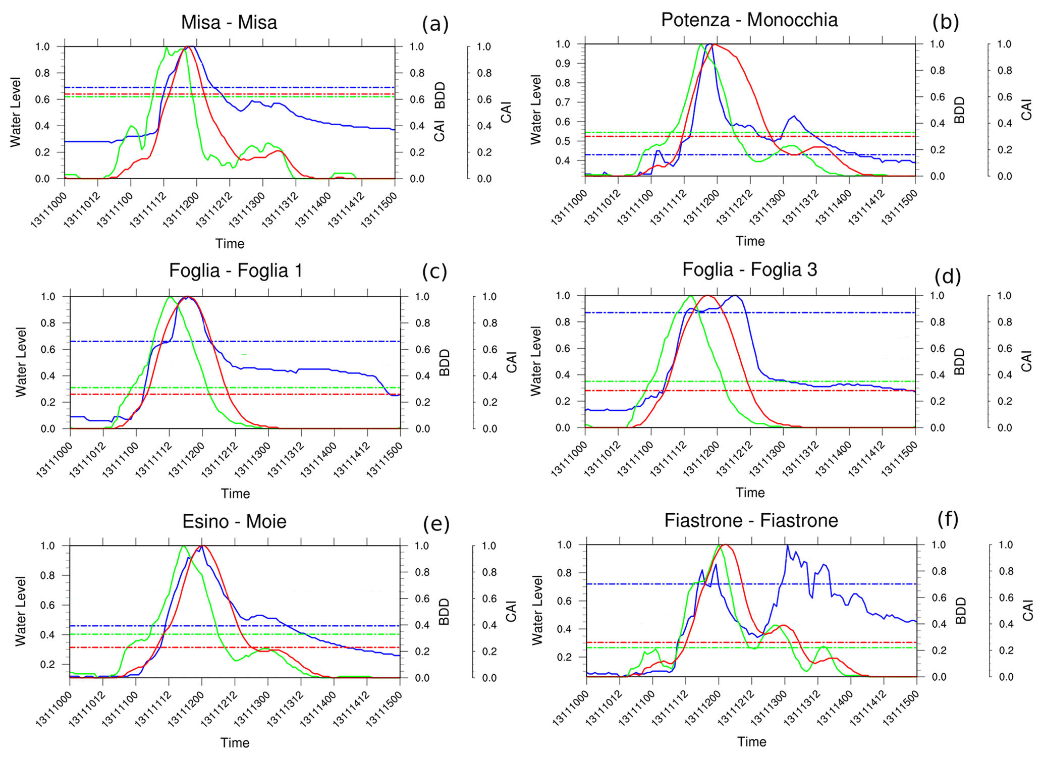
Figure 11 Time series comparison for six hydrometric stations: BDD hourly profile (red line), BDD moderate threshold (flat red line), CAI hourly profile (green line), CAI moderate threshold (flat green line), hydrometric-level hourly profile (blue line) and hydrometric-level moderate threshold (flat blue line). Quantity profiles and related thresholds are normalized.

5.2.3 Case study 3 – Abruzzo region

In the northern and central part of the Abruzzo region, precipitation amounts of up to 400 mm and 280 mm in 72 h were recorded in the Pretara and Castel del Monte rain gauges, respectively, over the inner, mountainous area (Fig. 7).

The main affected rivers (from north to south) were the Salinello, Tordino, Vomano, Piomba, Saline (including its tributaries Fino and Tavo) and Pescara, the latter one having the widest catchment of the region with a drained area of 3190 km². All catchments of the aforementioned rivers, as well as the whole Abruzzo region territory, are characterized by plenty of water withdrawals: according to ISPRA (2018), 14 relevant dams retain a total amount of 370.38×10⁶ m³ of water from the drainage network. An undefined number of minor withdrawals are still being counted by the local authorities (Abruzzo Regional Council Deliberation no. 435/2016), and the total magnitude of the water uptake is still difficult to assess.

Flood events for this case study affected the road networks, industrial settlements, and scattered houses located along the river paths and in depressed areas. Flood waves also occurred in the southern part of the region although they did not have significant effects. The main settings of CS03 (Fig. 6) are summarized in Table 4. The hydrological model assimilated data from 135 rain gauges from the official network. The comparison between 24 h index maps (Fig. 12) and ODB observation spatial distribution (Fig. 4) reveals a correspondence between the most damaged area, involving the entire north of the Pescara river system, and the highest hydrological stress, highlighted by the reddish colours. However, the CAI map also shows high hydrological stress in those southern watersheds, where inundations are not reported. On the other hand, according to the BDD map, no relevant stress is detected in this area. Moreover, the smallest tributaries were not highlighted by the latter index, coherently with CS01 and CS02 findings. In Fig. 13, six relevant normalized time series of hydrometric levels and indices are reported. The Tordino, Pescara and Vomano stations show peak shifting, due to the presence of many dams along the rivers' paths. For example, the Aterno-Pescara catchment hosts at least seven different dams, concentrated in a drained area of barely 3100 km². The induced flood shift may be even on the order of more than 1 d (e.g. 30 h delay in the Pescara a Villareia station, Fig. 11f). The Picciano and Fino watersheds are small, not impacted by human activity in terms of water uptake: in this case timing scores assume lower values (LTP and CTD are about 2 h for BDD and −1 h for the CAI, with RLTP of −0.29 and −0.14, respectively). DDTW results are 0.09 for BDD and 0.11 for CAI.

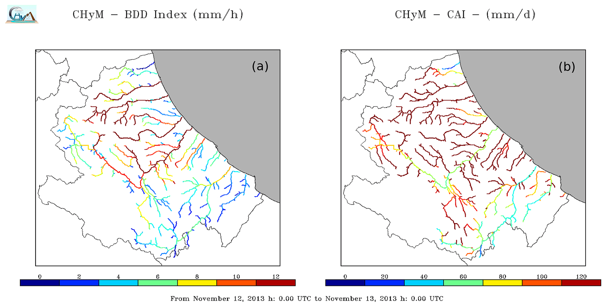
Figure 12 CS03 24 h maps of the BDD index (a) and the CAI (b) obtained for 12 November 2013, by forcing CHyM with observed rainfall data. Warmer colours indicate river segments with higher flood stress. In both figures, the Abruzzo region drainage network, belonging to the Central Apennine District, is highlighted.

Figure 13 Time series comparison for six hydrometric stations: BDD hourly profile (red line), BDD moderate threshold (flat red line), CAI hourly profile (green line), CAI moderate threshold (flat green line), hydrometric-level hourly profile (blue line) and hydrometric-level moderate threshold (blue flat line). Quantity profiles and related thresholds are normalized.

Among all the sensors analysed, the indices reported the right state of criticality for about 77 % of them (CR scores, Table 5).

Timing analysis is given for 26 hydrometric time series, located over 16 different river basins. The overall accuracy for CS03 is more than 0.9 for both indices, with a higher POD for BDD (0.81) than for CAI (0.72). However, the latter shows a slightly lower FAR. The LTP is about −8 for BDD and −12 h for the CAI, resulting in an RLTP of −1.1 for BDD and −1.6 for the CAI. The correlation time delay is lower for BDD than for CAI (−4.2 and −7.5, respectively), while the DDTW is very low for both the proposed alarm indices, as it is 0.09 for BDD and 0.1 for the CAI. Obtained results suggest that almost all flooding was predicted by both indices, even if the timing analysis reveals slight anticipation, probably due to the effect of artificial water management.

6 Conclusions

This work focused on flood prediction through the application of end-user-oriented indices, which are able to identify segments of drainage networks susceptible to flood. Several severe hydro-meteorological events, collected during the CETEMPS operational activity, were used to calibrate two hydrological index thresholds, starting from the calculation schemes of CHyM. The use of deterministic models for hydrological forecast involves a series of critical points: first of all, the need to calibrate and validate the model outputs with a very long time series of hydrological quantities, mainly represented by discharge data. However, these data are not always available, in particular, on small seasonal streams that are not remotely monitored but frequently hit by destructive flooding phenomena. Since flooding events are complex, depending on several processes, it is not straightforward to establish a flow discharge threshold value, beyond which the river can be considered susceptible to flood. For this reason, many hydrological thresholds that have been developed are site-specific and not generally applicable over different areas, other than the river sections where they have been calibrated. The two proposed indices, the CAI and BDD index, were validated on a case study basis, through the analysis of an extreme weather event affecting Central Italy on 11–13 November 2013. The 3 d event was simulated by the Cetemps Hydrological Model, forced with observed rain gauge data, over three different geographical domains encompassing the Umbria and Tiber basin, Marche, and Abruzzo regions. Index formulations followed two different approaches: the BDD index is based on the ratio between the computed (natural) discharge and the square of the hydraulic radius, while the CAI is more empirical, representing the amount of precipitation drained at each grid point of the drainage network, in a time interval corresponding to the mean time of concentration of the upstream area. Three thresholds have been set for each index and calibrated in order to obtain a qualitative correspondence between the indices and the hydrometric threshold exceedances, defined by each regional Civil Protection functional centre. A colour code, similar to those used for the hydrogeological criticality assessment, was then assigned to each threshold, with the aim of simplifying index signal interpretation by Civil Protection end-users. The forecast skill of both indices has been investigated at the station level, through dichotomous and continuous statistical analysis, by comparing indices' time evolution and hydrometric-level time series, taking advantage of typical assessment methods used in signal theory, such as derivative dynamic time warping. Moreover, spatial information given by both indices was assessed by comparing daily BDD and CAI stress maps and localization of effects on the ground, collected from event reports, press releases and warnings. Results obtained indicated that the hydrological-stress spatial information, highlighted by higher index values, is coherent with the localization of affected municipalities and flood reports, while no stress overestimation is reproduced over those areas not involved in the event. Objective dichotomous statistical analysis was performed over 78 hydrometric stations by using contingency tables, built by comparing indices and hydrometric-height moderate-threshold exceedances. Results evidenced high accuracy, with values exceeding 0.8 for both indices and all CSs. False alarm rates were under 0.5, while an appreciable difference is given by the probability of detection, ranging from 0.51 for the CAI to 0.80 for BDD among the different case studies. Signal analysis has been carried out over 120 h time series of indices and observed river stages. The DDTW over all stations was found to be abundantly lower than 0.1, which is commonly referred to as the threshold value beyond which two signals can be considered independent. Even if the stress signal behaviour was correctly reproduced by both indices, peak timing analysis showed some anticipation in signal peak occurrences on the order of few hours. Timing bias is more pronounced for the CAI, where displacements of more than −4 and up to about −7 h are highlighted by all statistical parameters. As mentioned, validation scores were calculated considering all available hydrometers in the domain; however, it should be highlighted that the greatest number of the considered stations are placed downstream of dams. Therefore, in these points, flood propagation is heavily influenced by retention and release from artificial water storage, which is widespread over the geographical domain considered and heavily exploited in terms of hydroelectric power production. Index performance would benefit from the potential availability of retention and release data; however, the main aim of developing general thresholds for the proposed indices deals with contemplating data scarcity and the hypothesis of unavailability of information about water uptake, which is very difficult to find, in the authors' experience. As for the indices' applicability, results highlighted a different index response to different catchments and diverse flooding dynamics. According to Chen et al. (2010), floods may have different drivers: fluvial floods are mainly determined by the limited capacity of drainage systems, while pluvial floods are caused by deluges from river channels. However, the discrimination between a pluvial and a fluvial flood is not sharp; as a matter of fact, most events result in a combination of both processes. This condition often affects small hydrological basins, such as most Italian rivers (drained area lower than 10 000 km², according to the definition provided by Chapman, 1992). According to the underlined differences found in CAI and BDD mapping, the proposed indices give complementary information about hydrological stress over wide areas, as the CAI appears to be more responsive to predominant pluvial flood dynamics affecting the smallest tributaries, while higher stress identified by BDD occurs over main channels.