the Creative Commons Attribution 4.0 License.
the Creative Commons Attribution 4.0 License.
 | 07 Jan 2021
The role and value of distributed precipitation data in hydrological models
Markus Hrachowitz
Malte Neuper
Erwin Zehe
This study investigates the role and value of distributed rainfall for the runoff generation of a mesoscale catchment (20 km2). We compare four hydrological model setups and show that a distributed model setup driven by distributed rainfall only improves the model performances during certain periods. These periods are dominated by convective summer storms that are typically characterized by higher spatiotemporal variabilities compared to stratiform precipitation events that dominate rainfall generation in winter. Motivated by these findings, we develop a spatially adaptive model that is capable of dynamically adjusting its spatial structure during model execution. This spatially adaptive model allows the varying relevance of distributed rainfall to be represented within a hydrological model without losing predictive performance compared to a fully distributed model. Our results highlight that spatially adaptive modeling has the potential to reduce computational times as well as improve our understanding of the varying role and value of distributed precipitation data for hydrological models.
- Article
(3048 KB) - Full-text XML
-
Supplement
(367 KB) - BibTeX
- EndNote


“How important are spatial patterns of precipitation for the runoff generation at the catchment scale?” This is a key question for the application of hydrological models that has been addressed in several studies over the past decades (e.g., Beven and Hornberger, 1982; Smith et al., 2004; Lobligeois et al., 2014). A frequently drawn conclusion is that semi-distributed or even lumped models driven by a single precipitation time series often outperform distributed models with respect to their ability to reproduce observed streamflow at the outlet of a catchment (e.g., Das et al., 2008). Although the generality of such findings is surely limited by the fact that distributed models have more parameters that need to be identified, which makes model calibration much more challenging (Beven and Binley, 1992; Huang et al., 2019), they highlight the ability of the hydrological system to dissipate spatial gradients efficiently (e.g., Obled et al., 1994). This is the case as hydrological processes are strongly dissipative but exhibit, despite the nonlinearity of surface and subsurface flow processes, no chaotic behavior (Berkowitz and Zehe, 2020).
In contrast to the above-mentioned finding that hydrological systems can efficiently dissipate spatial gradients, several other studies showed that information about the spatial variability of precipitation can significantly improve the predictive performance of hydrological models. For instance, Euser et al. (2015) highlighted that distributed models driven by distributed rainfall could reproduce the observed hydrograph of a 1600 km2 large catchment in Belgium with higher accuracy compared to spatially lumped model structures. Furthermore, Woods and Sivapalan (1999) showed that the interplay between spatial patterns of rainfall and soil saturation can substantially impact the runoff generation of a catchment when they analyzed the dependence of average runoff rates on the spatial and temporal variability of the meteorological forcing and the catchment state. The relevance of these spatial patterns is thereby particularly high if the system is close to a threshold where different localized preferential flow processes start to dominate (e.g., cracking soils: drying of soil; macropores: occurrence of earthworms) as discussed by Zehe et al. (2007). Spatial averaging of the system state or the meteorological forcing can hence lead to a misrepresentation of relevant spatial patterns, especially at more extreme conditions.
Given the partly contradictory findings present in the literature, it appears reasonable to assume that the relevance of distributed rainfall is changing dynamically over time and depends on the interplay of the prevailing (i) system state (e.g., catchment wetness); (ii) the system functional structure, determined by patterns of topography, land use, and geology; and well as (iii) the strength and spatial organization of the rainfall forcing. In consequence, it seems furthermore rational to hypothesize that also hydrological models should dynamically adapt their spatial structure to the prevailing context, thereby reflecting the inherently dynamic nature of hydrological similarity (Loritz et al., 2018).
The idea that hydrological models should dynamically allocate their spatial resolution, as well as the associated representation of natural heterogeneity in time, is motivated by our previous work (Loritz et al., 2018). In that study, we highlighted that simulations of a distributed model consisting of 105 independent hillslopes were highly redundant to reproduce discharge or catchment storage changes of a mesoscale catchment within 1 hydrological year. Based on the Shannon entropy as a metric, we identified periods in which a rather small number of representative hillslopes was sufficient because most of them functioned largely similarly within the chosen margin of error. However, during other periods, up to 32 independent representations of hillslopes were required, which underlines that spatial variability of system properties, such as surface topography or soil types among the hillslopes, can exert a stronger influence on the runoff generation at certain times, as expected given the findings reported by other studies conducted in the same research environment (e.g., Fenicia et al., 2016; Loritz et al., 2017). It can, therefore, be argued that distributed rainfall and corresponding distributed model structures are also only important during specific periods, while during other periods a compressed, spatially aggregated model structure may be sufficient. An implementation of such an adaptive spatial model resolution would ensure an appropriate spatial model complexity, defined based on the least number of details about the system structure (e.g., the variability of topographic gradients) and catchment states that are sufficient to capture the relevant interactions with the spatial pattern of precipitation. Yet it would be as parsimonious as possible to avoid redundant computations, which again could be used to minimize computational costs (Clark et al., 2017).
Moving to the event timescale instead of running continuous simulations is surely one way to achieve such a dynamical allocation of the model space and means to use different model setups with different spatiotemporal resolutions at different times. This would entail running a set of models that differ with respect to their resolutions in space and time, depending on the prevailing structure of the meteorological forcing and current state of a hydrological landscape (e.g., the soil moisture or energy state). Yet, this introduces multiple new problems, for instance, how to infer the initial conditions of a catchment prior to a rainfall event given the degrees of freedom distributed models can offer (Beven, 2001). The latter is of considerable importance, particularly during extremes resulting from high-intensity rainfall-runoff events, which can be strongly sensitive to the actual state of the system such as the spatial patterns of macropores (Zehe et al., 2005) or of the antecedent soil water content (Zehe and Blöschl, 2004).
A different avenue to implement a dynamically changing model resolution is adaptive clustering, as recently demonstrated for a spatially distributed conceptual (top-down) model by Ehret et al. (2020). This concept allows for continuous hydrological simulations, which use a higher spatial model resolution only at those time steps when it is necessary. The idea behind adaptive clustering is similar to adaptive time stepping (e.g., Minkoff and Kridler, 2006). However, instead of reducing the time steps during times when large gradients prevail, adaptive clustering increases or decreases the number of independent spatial model elements during times of low or high functional diversity. The general concept behind adaptive clustering is thereby not entirely new to environmental science and is already used for instance in hydrogeology under the term “adaptive mesh”, with the main focus to increase the resolution of gradients during times of high dynamics by increasing or decreasing the number of nodes (grid elements) in a model (Berger and Oliger, 1984). The main difference between the adaptive mesh and adaptive clustering approach is that instead of adjusting the spatial resolution of the numerical grid during runtime, adaptive clustering changes the number of hydrological response units (HRUs) that are used (needed) to represent a catchment. This implies that also the degree of spatial heterogeneity of the catchment state (e.g., the soil moisture or energy state) that is covered by the model is dynamically changing.
While the idea of adaptive clustering is promising as it allows a minimum adequate representation of the spatial variability of a hydrological landscape, it has, to the best of our knowledge, so far only been tested within a simple top-down model (Ehret et al., 2020). It is thus of interest whether such a dynamic clustering is also feasible when using a physically based (bottom-up) model particularly as these models were specifically introduced to explore how distributed system characteristics and driving gradients control hydrological dynamics (Freeze and Harlan, 1969). Here we will hence test and develop an adaptive clustering approach using straightforward physical reasoning and implement it into a distributed bottom-up model. The overarching objective of this study is thus to exploit the value of adaptive clustering as a tool to better understand the temporal relevance of distributed precipitation for the runoff generation of a mesoscale catchment and, as a by-product, to reiterate that adaptive clustering could potentially be used to reduce computational times, as already discussed in detail by Ehret et al. (2020). High computational times are thereby still one of the many reasons why bottom-up models are rarely used on larger scales in an spatial explicit manner (Clark et al., 2017). For instance, Hopp and McDonnell (2009) used the HYDRUS 3D model (e.g., latest version of HYDRUS; Šimunek et al., 2016) and reported computational times ranging from 10 min up to 11 h when they simulated water fluxes and state variables at the Panola hillslope (area = 0.001250 km2 (25 m × 50 m); maximal soil depths = 4 m) for a simulation time of 15 d by changing slope angles, soil depths, storm sizes, and bedrock permeability. A meaningful application of bottom-up models at relevant management scales (around 250 km2 in south Germany; e.g., Loritz, 2019), without a violation of important physical constraints (e.g., 10−2–101 m maximum vertical grid size for the Richards equation; Or et al., 2015; Vogel and Ippisch, 2008), would thus imply long computational times. This again strongly limits the number of feasible model runs to examine, for instance, different parameter sets (Beven and Freer, 2001).
In this study, we therefore test the specific hypothesis that adaptive clustering is a feasible approach to represent the spatial variability of rainfall in a hydrological bottom-up model at the lowest sufficient level of detail without losing predictive performance compared to a fully distributed model. We test this hypothesis by introducing a clustering approach for the example of the model CATFLOW applied to the 19.4 km2 Colpach catchment using a gridded radar-based quantitative rainfall estimate by addressing the two following research questions:
-
Does the model performance of a spatially aggregated model improve when it is distributed in space and driven by distributed rainfall?
-
Can adaptive clustering be used to distribute a bottom-up model in space that it is able to represent relevant spatial differences in the system state and precipitation forcing at the least sufficient resolution to avoid being highly redundant as a fully distributed model?
2.1 The Colpach catchment
The 19.4 km2 Colpach catchment is located in northern Luxembourg and is a headwater catchment of the 256 km2 large Attert experimental basin (Fig. 1). The prevailing geology of both catchments is Devonian schists of the Ardennes massif which are characterized by coarse-grained and highly permeable soils (>1 m; e.g., Jackisch et al., 2017; Juilleret et al., 2011). The steep hills of the Colpach are primarily forested, and the elevation of the Colpach ranges from 265 to 512 m a.s.l. Annual runoff coefficients varied around 50 % ± 7 % for the 2011–2017 period. Precipitation is rather evenly distributed across the seasons (vegetation and winter season), while the runoff generation has a distinct seasonal pattern as around 80 % of the annual discharge is released between October and March (Seibert et al., 2017). The Colpach and its sub-catchments (e.g., Weierbach) have been used as study area in a series of scientific publications. We refer here to Pfister et al. (2018), Jackisch (2015) or Loritz et al. (2017) for a more detailed system description (mean annual precipitation: 900–1000 mm yr−1; mean annual evapotranspiration: 450–550 mm yr−1; mean annual discharge: 450–550 mm yr−1; land use: 65 % forest, 23 % agriculture, 2 % others; mean annual temperature: 9.1 ∘C).
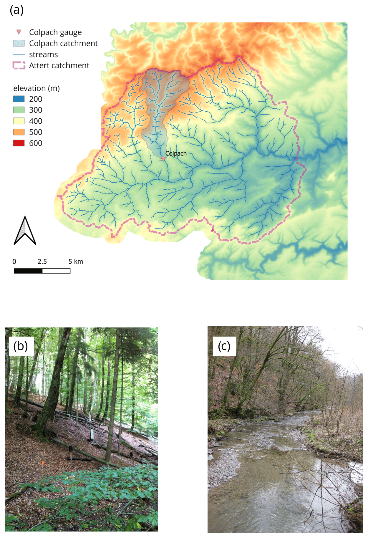
Figure 1(a) Map of the Colpach catchment (location northern Luxembourg), (b) picture of a typical forested hillslope within the Colpach catchment, and (c) the Colpach River around 4 km north of the gauging station.
2.2 The CATFLOW model
The key elements of the CATFLOW model (Maurer, 1997; Zehe et al., 2001) are 2D hillslopes which are discretized along a two-dimensional cross section using curvilinear orthogonal coordinates. Evapotranspiration is represented using an advanced SVAT (soil–vegetation–atmosphere transfer) approach based on the Penman–Monteith equation, which accounts for tabulated vegetation dynamics, albedo as a function of soil moisture, and the impact of local topography on wind speed and radiation. Soil water dynamics are simulated based on the Darcy–Richards equation (solved implicitly, modified Picard iteration; Celia et al., 1990), and surface runoff is represented by a diffusion wave approximation of the Saint-Venant equations using adaptive time stepping (solved explicitly, Euler forward starting downslope). Vertical and lateral preferential flow paths are represented as connected pathways containing an artificial porous medium with high hydraulic conductivity and very low retention. The hillslope module is designed to simulate infiltration excess runoff, saturation excess runoff, re-infiltration of surface runoff, lateral water flow in the subsurface, and return flow but cannot handle snowfall or snow accumulation. The latter means that CATFLOW should not be applied if snow is a dominant control, which is not the case in the Colpach catchment. The model core is written entirely in FORTRAN77, and the individual hillslopes can be run in parallel on different CPUs to assure low computation times and high performance of the numerical scheme. Up-to-date model descriptions can be found in Wienhöfer and Zehe (2014) or in Loritz et al. (2017).
2.3 Meteorological forcing and observed discharge
Meteorological input data used here are recorded at a temporal resolution of 1 h at two official meteorological stations by the “Administration des Services Techniques de l'Agriculture Luxembourg” at the locations Roodt and Useldange. The meteorological station Roodt measures rainfall within the catchment border (Fig. 2a) and provided the precipitation input to the model of Loritz et al. (2017). The second station Useldange, located outside the catchment around 8 km west of the Colpach outlet, measures air temperature, relative humidity, wind speed, and global radiation. These data are used as meteorological input (except for precipitation) in all model setups in this study. In other words, this means that all model setups in this study are forced by identical meteorological inputs, except for the precipitation data (see Sect. 3.1). Therefore, we cannot account for variations of the wind speed or the temperature within the Colpach catchment. A detailed description and analysis of the meteorological data can be found in Loritz et al. (2017).
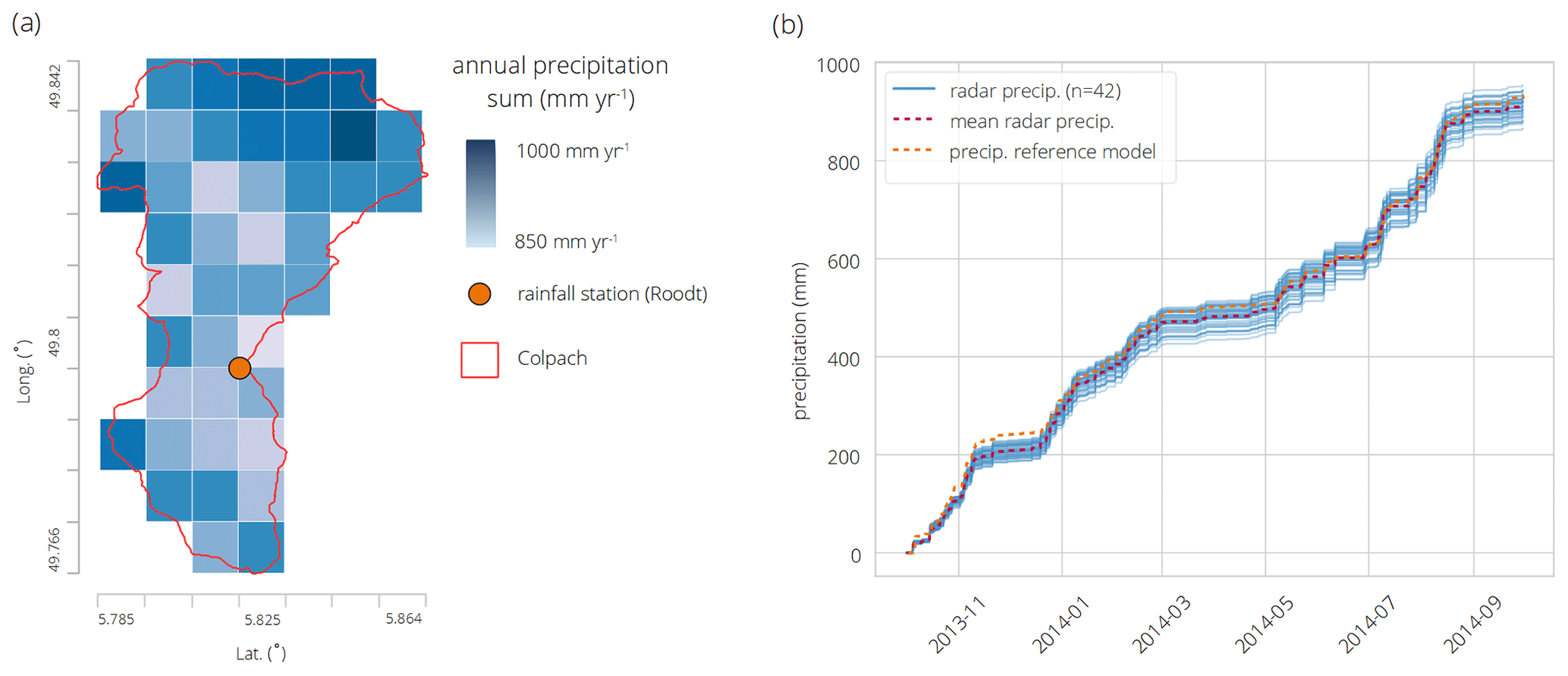
Figure 2Annual sums of the gridded precipitation field over the Colpach catchment for the hydrological year 2013/14 as well as the location of the rainfall station Roodt, which is used as precipitation input for the reference model (spatial resolution: 1 km2; coord. system WGS84) (a). Cumulated precipitation for each grid cell for the hydrological year 2013/14 of the precipitation field (blue lines), the corresponding mean of the precipitation field (dashed red line) and the precipitation data from the station in Roodt (b, dashed orange lines).
Discharge observations of the Colpach are provided by the Luxembourg Institute of Science and Technology (LIST) in a 15 min temporal resolution for the hydrological year 2013/14. The data were aggregated to an hourly temporal resolution and to specific discharge given the catchment area of 19.4 km2.
2.4 Spatially resolved precipitation data
Besides the precipitation data from the ground station located in Roodt, we use a gridded quantitative precipitation estimate, which is a merged product of two weather radars, rain gauges, micro rain radars, and disdrometer observations (location of the ground measurements in the Supplement and in more detail in Neuper and Ehret, 2019). The two radar stations used are located 40 to 70 km and 24 to 44 km away, respectively, from the borders of the Attert catchment (Neuheilenbach, Germany; Wideumont, Belgium) and are operated by the German Weather Service (DWD) as well as by the Royal Meteorological Institute of Belgium (RMI). Both distances are within a range that the data can be used at a high resolution of 1×1 km as the signal is neither degraded by beam spreading nor impacted by partial blindness through cone of silence issues (Neuper and Ehret, 2019). The raw data, 10 min reflectivity data from single polarimetric C-Band Doppler radar, were aggregated to hourly averages and filtered by static, Doppler clutter filters and bright-band correction following Hannesen (1998). Second trip echoes and obvious anomalous propagation echoes were manually removed, and the corrected data were used to create a pseudo plan position indicator data set at 1500 m above the ground. A more detailed description of how the reflectivity data were transformed to rainfall data and calibrated as well as validated against rain gauges, micro rain radars, and disdrometers can be found in the Supplement and in Neuper and Ehret (2019).
The chosen precipitation time series starts on 1 October 2013 and ends on 30 September 2014. 42 grid cells (1×1 km) of the precipitation field intersect with more than 50 % of their area with the Colpach catchment and are used in this study (Fig. 2a). The weather radar measured an area-weighted mean of around 900 mm yr−1 in the Colpach catchment for the selected period. This is in accordance with the reported climatic averages (900–1000 mm yr−1) of this region (Pfister et al., 2017). The maximum hourly precipitation difference between the grid cells in the study period is 14 mm h−1 (August 2014), and the maximum annual precipitation difference between the grid cells is 95 mm yr−1 (Fig. 2b). Temporally, the precipitation distributes evenly over the year, with around 50 % of rainfall in winter and 50 % of rainfall in summer with a short dry spell from mid-March to the end of April. There is a weak correlation between the mean elevation of the grid cells and the annual precipitation sums of 0.43. This implies that precipitation tends to be slightly higher in the northern parts of the catchment that are also characterized by higher altitudes (Fig. 2a). The measured precipitation time series from the ground station located in Roodt differs from the mean precipitation of the spatial rainfall field about 30 mm yr−1 and around 60 mm yr−1 from the exact location in the precipitation grid measured by the weather radar, with a tendency of higher rainfall values especially in the winter season. Why exactly the precipitation observations of the ground station in Roodt differ in this magnitude from the merged product of the weather radar is an interesting research question, however, not within the scope of this study.
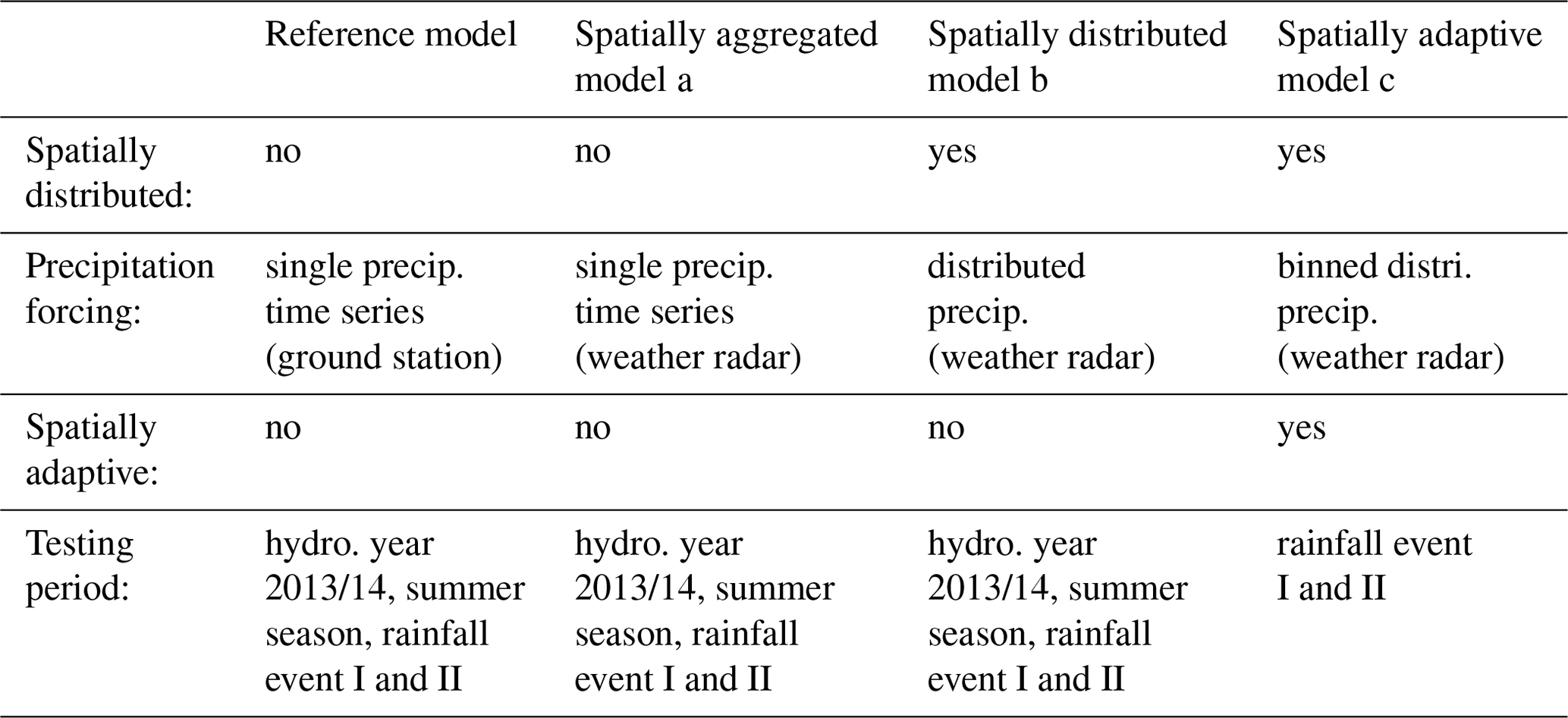
In Sect. 3.1 to 3.3, we introduce three non-adaptive model setups (reference model, model a, and model b) and a spatially adaptive model setup (model c). Details on how the model setups are tested are provided in Sect. 3.4 and 3.5. A summary of the different model setups can be found in Table 1.
3.1 The reference model of Loritz et al. (2017)
All model setups in this study are based on a spatially aggregated model structure (reference model), developed and extensively tested in the Colpach catchment in a previous study (Loritz et al., 2017). The general idea behind the proposed model concept (representative hillslope) is that a single bottom-up hillslope model reflects a meaningful compromise between classical top-down and bottom-up models (Hrachowitz and Clark, 2017; Loritz, 2019). This is because a representative hillslope resolves the effective gradient and resistance controlling water storage and release and allows macroscopic model parameters to be derived from available point measurements. The parameters of the model of Loritz et al. (2017) were, for the most part, derived directly from a large amount of field data, and the model was only manually fine-tuned afterwards by further exclusively adjusting the spatial macropore density within a few trial and error runs to simulate the seasonal water balance of the Colpach catchment. The model simulations were tested against hourly discharge observations on an annual and seasonal timescale, against discharge observations from a sub-basin of the Colpach, in a different hydrological year, against hourly soil moisture observations (38 sensors in 10 and 50 cm depth), and with hourly normalized sap flow velocities (proxy for transpiration; 30 sensors). The developed model structure agreed well with the dynamics of the observables and showed higher model performances as reported in other studies working with different top-down model setups in the same environment (Wrede et al., 2015).
To summarize, the reference model serves as a benchmark here to (a) evaluate the other models and (b) provide the structural basis for them. None of the other model setups are further calibrated or manually tuned, and the only difference between the different model setups is the precipitation data they are driven with and their model resolution. For further details on how the reference model was set up and tuned, we refer to the study of Loritz et al. (2017).
3.2 Non-adaptive models a and b
Despite the acceptable annual model performance of the reference model, it showed deficits in simulated runoff response to a series of summer rainfall-runoff events. As discussed in Loritz et al. (2017), one possible explanation for the unsatisfying performance is that summer precipitation in the Colpach catchment is mainly driven by convective atmospheric conditions. These convective precipitation events are characterized by a much smaller spatial extent as well as by higher rainfall intensities compared to the stratiform and frontal precipitation events that dominate during winter (Neuper and Ehret, 2019). The insufficient model performance in summer could therefore likely be a consequence of the larger spatial gradients of the rainfall field compared to the winter season that cannot be accounted for in the original model of Loritz et al. (2017). In other words, this necessitates that a hydrological model, distributed at a sufficiently high spatial resolution, is required to capture the spatial variability of the precipitation field to achieve improved simulations of the runoff generation of the Colpach. One goal of this study (first research question) is hence to test the hypothesis as to whether the performance deficiencies of the representative hillslope model, the reference model, in summer are mainly caused by the inability of the setup to account for the spatial variability of the precipitation field.
To address the first research questions of this study (“Does the model performance of a spatially aggregated model improve if it is distributed in space and driven by distributed rainfall”), we analyze simulations of two alternative model setups (model a and model b), additional to the reference model from Loritz et al. (2017). Both model setups are described in detail below.
3.2.1 Spatially aggregated model a
Model a is structurally identical to the reference model; however, it is driven by the area-weighted mean of the spatially resolved precipitation data described in Sect. 2.4 and plotted in Fig. 2b. We used the area-weighted mean as not all raster cells of the distributed precipitation data are entirely within the borders of the Colpach catchment. This means that the weight of a grid cell which is not entirely located within the catchment is reduced when we calculate the average according to the percentage areal overlap.
We added model a to test if the performance difference between the reference model and our distributed model b is merely a result of quantitative differences between the different precipitation products measured either by a single ground station or by a weather radar in combination with different ground stations.
3.2.2 Spatially distributed model b
Model b is a spatially distributed version of the reference model. More specifically, here all model parameters of the representative hillslope (reference model), as well as all other meteorological variables such as temperature or wind speed, are identical to the reference model. However, model b is spatially distributed as well as driven by distributed rainfall data. This model setup is distributed on the spatial resolution of the precipitation field similarity, as done for instance by Prenner et al. (2018) and not following the traditional spatial discretization strategy of CATFOW based on a fixed number of hillslopes, inferred from surface topography or land use. Model b thus represents the Colpach with 42 spatial grids (1×1 km). In each of these grids, we run a model identical to the reference model, however, driven with the specific precipitation data measured at this location.
We justify this assumption based on the model validation in Loritz et al. (2017) and on a study conducted in the same research environment (Loritz et al., 2019), where we showed that different sub-basins of the Attert catchment (the Colpach is a headwater catchment of the Attert catchment) have similar specific discharges as long as they are located in the same geological setting and are driven by a similar meteorological forcing (see also Sect. 4.2).
3.3 Spatially adaptive model c
To address the second and main research question of this study (“Can adaptive clustering be used to distribute a bottom-up model in space that it is able to represent relevant spatial differences in the system state and precipitation forcing at the least sufficient resolution to avoid being highly redundant as a fully distributed model?”), we develop a third adaptive model setup (model c). This spatially adaptive model setup is based on the distributed model b, however, is able to dynamically adjust its spatial structure in time based on the precipitation forcing, as detailed in Sect. 4.1 to 4.3.
3.4 Model testing – non-adaptive models a and b
We analyze the simulation performances of model a (spatially aggregated) and b (spatially distributed) by calculating the Kling–Gupta efficiency (KGE; Kling and Gupta, 2009) and analyze its three components (see Supplement) between the hourly discharge simulations of the individual model setups against hourly observed discharge at different timescales (annual, seasonal, event scale). Model a and b are run for the hydrological year 2013–2014 with hourly printout times and differ only concerning the precipitation data they are driven with:
-
model a: driven by an area-weighted mean of the spatially resolved precipitation data;
-
model b: driven by 42 precipitation time series, each reflecting a grid cell of the precipitation field shown in Fig. 2.
To be able to compare the discharge of the spatially aggregated model a and the distributed model b with the observed discharge of the Colpach catchment and to account for the routing of the water from a specific location to the outlet, we added a simple lag function acting as the channel network. The latter is based on the average flow length along the surface topography of each precipitation grid to the outlet of the catchment assuming a constant flow velocity of 1 m s−1 (e.g., Leopold, 1953). The flow length of each grid is estimated based on a 10 m resolved digital elevation model. For the spatially aggregated model a, we average all flow distances to the outlet and shift the single discharge simulation accordingly.
3.5 Model testing – adaptive model c
We test the spatially adaptive model c for two selected rainfall-runoff events, which are characterized by distinctly different precipitation properties. We chose event I as it has the highest intensity and third-highest spatial variability in summer and event II because it is the event with the longest continuous precipitation in the time series. Both events were picked to represent the spectrum of rainfall events in the summer season. We focus exclusively on the summer season as the distributed model b only outperforms the reference model in this period, indicating that spatially distributed rainfall provides no performance-relevant information during winter. A full automation of the proposed adaptive clustering approach is beyond the scope of this study, and we focus here on the introduction as well as the physical underpinning of the approach.
The main goal of testing the spatially adaptive model c is to show that we can achieve similar simulation results compared to the fully distributed model b, however, with a reduced number of hillslopes (coarser resolution). We therefore calculate not only the KGE between the simulated discharge of model c with the observed discharge at event I and II but also the KGE between the simulated discharge of model c and the simulated discharge of model b on an hourly basis. A full automation of the proposed adaptive clustering approach and a test on a longer timescale are beyond the scope of this study, and we point towards the study of Ehret et al. (2020), who have shown the potential of adaptive clustering using a conceptual model, also for longer periods.
Spatially adaptive modeling or adaptive clustering is an approach to dynamically adjust the spatial structure of a hydrological model in time, offering the possibility to reduce computational times as well as to find an appropriate, time-varying spatial model resolution (Ehret et al., 2020). The basic idea of adaptive clustering has been motivated within the work of Zehe et al. (2014), who stated that functional similarity in a catchment (or in a model) can only emerge if different sub-units are structurally similar (e.g., topography, geology, land use), are driven by a similar forcing, and are at a similar state. The latter implies that the concept of hydrological similarity, frequently used as the basis to discretize a catchment in space (e.g., Sivapalan et al., 1987), cannot be time-invariant but needs to dynamically change in time (Loritz et al., 2018). This is the case as the relevance of different spatial controls like the topography or pedology of a catchment depends on the prevailing state and forcing (Woods and Sivapalan, 1999). A suitable discretization of a catchment into similar functional units needs hence to be time-variant, and one way to achieve such a dynamic model resolution is spatially adaptive modeling.
Implementing adaptive clustering into a distributed model requires specific decision thresholds that define whether spatial differences in the structure, forcing, and state of sub-units (e.g., hillslopes, sub-basins) are so large that they need a distributed representation. This means that if differences between the structure, forcing, or state of two or more distributed model elements (here gridded models) are below these thresholds they are by definition similar, which means that they can represent each other's hydrological function. The concept that certain spatial model elements can represent other model elements is not new and has been used frequently in hydrology since at least Sivapalan et al. (1987), who introduced the concept of representative elementary areas. The novelty of adaptive clustering is that hydrological similar model elements are dynamically grouped and split in the runtime of the model instead of running a constant number of model elements for the entire simulation period (Ehret et al., 2020).
4.1 Spatially adaptive modeling – similarity assumption
Identifying periods when a model element can represent another one because it functions hydrologically similarly is the main challenge of adaptive clustering. For this purpose, we subdivide the precipitation field and the model states at each time step into equally distant bins (bins = groups) and classify those as similar that occupy the same bin. If two or more observations or models are hence in the same bin, they are by our definition functionally similar and can represent each other. To give an example, imagine if 50 % of the catchment area receives precipitation of around 1 mm h−1 and 50 % around 2 mm h−1. In this specific case, we would have two occupied forcing bins (precipitation groups; PB). In the following, we explain how we have chosen the decision thresholds for the system structure, the precipitation forcing, and the model states.
4.1.1 Time invariant similarity of the system structure
The first step of our adaptive clustering approach requires the identification of hydrological response units (HRUs) that potentially behave similarly. These similar units are typically identified based on structural properties such as the geological setting, the land use, or the topography. The general idea is that HRUs are grouped together which share the same controls on gradients and resistances controlling flows of water as long as they are in the same state (Zehe et al., 2014). As already mentioned in Sect. 3.2, our previous studies showed that different sub-units of the Colpach catchment are characterized by similar spatially organized surface and subsurface characteristics (integral filter properties). This entails a potential similar rainfall-runoff transformation when they are in a similar state. The latter is supported by our previous work (Loritz et al., 2017, 2019), which revealed that a sub-basin of the Colpach catchment (0.45 km2) and a neighboring catchment (30 km2) located in the same geological setting have almost identical specific discharges as long as they are at similar states and forced by comparable amounts of precipitation. We hence assume that all grid cells of the precipitation field can thus be represented by the same model with the same model parameters as long as they are in the same state and driven by the same forcing. This necessitates, however, also that if we extend our research area to a catchment that is divided, for instance, into two or more geological settings and different dominant land use or soil types that function hydrologically differently (regarding their integral filter properties), we need to run two or more structurally different models. Each of these models represents thereby a unique structural setting. The latter might limit the possibilities to apply this approach on larger scales or in areas with complex structural settings.
4.1.2 Time-variant similarity of the precipitation forcing
The second decision threshold we need to identify defines the minimum difference at which we consider differences in the precipitation field as relevant for the runoff generation. Simply speaking, two structurally similar hydrological units that are in the same state will only respond differently to an external forcing if the variability in the forcing has exceeded this threshold. Here, we picked a threshold of 1 mm h−1 upon which we consider differences between precipitation observations (grid cells) as relevant. We chose this threshold as a reasonable value for which we expect differences in hydrologic behavior in this humid catchment and based on our collective understanding of the Colpach catchment. This means that only if the spatial differences in the precipitation field are above 1 mm h−1 do we drive the spatially adaptive model c with different precipitation inputs. The choice of this threshold is important, as it is one of two main controls or parameters of the model resolution of the spatially adaptive model (see Supplement B).
4.1.3 Time-variant similarity of the catchment state
The third assumption is to identify a decision threshold upon which we consider that two model elements are in the same state. This means that we need to select a point in time after a spatially variable rainfall event (>1 mm h−1) when two or more model elements in the individual grid cells have dissipated the differences between them introduced by the previous precipitation input with drainage and evapotranspiration dynamics. Here, we use the change in discharge over time (dQ dt−1; slope of the simulated hydrograph) and the discharge (Q) at a time step to infer similar model states. By that, we expect that two or more gridded models are again in the same state if the individual models estimate runoff and the slope of the runoff within a 0.05 mm h−1 margin. As soon as this is the case and two or more gridded models are in the same state, we average their states (average saturation of each grid cell of the CATFLOW hillslope grid) and, by that, aggregate the models back again into a one hillslope. The value of 0.05 mm h−1 for Q and dQ dt−1 was picked as it reflects the desired precision of the adaptive model c. Similar to the case of the decision threshold, this value needs to be picked carefully. Furthermore, it is important to choose similarity metrics (here dQ dt−1 and Q) that adequately describe the model states during the simulation time.
4.2 Spatially adaptive modeling – model implementation
As stated in Sect. 3.1, we classified the entire Colpach catchment as hydrologically similar with respect to the runoff generation as long as the different hydrological sub-units of the catchment are in the same state and receive a comparable forcing. This means that we start the simulation with one gridded hillslope to represent the entire catchment and continue in this mode as long as we have not detected a spatial difference in the precipitation field above the selected threshold of 1 mm h−1 (Fig. 3, t=0). At each time step, we bin the precipitation input of the next time step and determine the number of allocated bins (PB is the number of precipitation bins). If more than one precipitation bin is occupied (PB > 1), we increase the number of gridded models (M is the number of running gridded models) by running the same model in the same initial state, however, driven by different precipitation inputs.
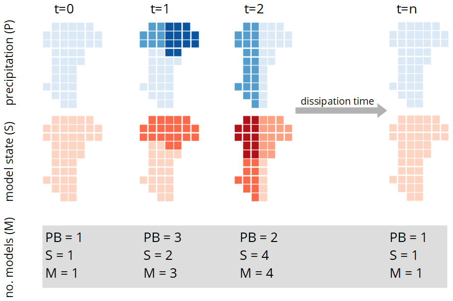
Figure 3Sketch of the spatial adaptive modeling described in Sect. 4.2. The upper panel shows the precipitation forcing (blue) and the lower panel the model states (red). The numbers below the figures indicate how many precipitation (PB) and model state (S) bins (groups) are occupied and how many models (M) are running at the given time step.
Consider a scenario in which the Colpach catchment is represented by one hillslope (S=1), and we observe a precipitation event in which 50 % of the catchment receives no precipitation, 20 % 7 mm h−1 and 30 % 8 mm h−1, as displayed in an illustrative example in Fig. 3 at t=1. This would mean that three precipitation bins are allocated (PB = 3), and we need to increase the number of running models to three (M=3). After running these three models for one time step with the different precipitation inputs, we bin the model states (dQ dt−1; Q). Let us assume we would identify two occupied model state bins, which means that two different model states (S=2) are needed to represent the spatial variability of catchment states. This could happen if the differences between the 7 and 8 mm h−1 rainfall intensity did not result in a significant difference in the discharge simulation of the two corresponding models. Following our approach, we aggregate the two models that are driven by 7 and 8 mm h−1 by averaging their states. We do this by averaging the relative saturation of the corresponding CATFLOW hillslope grids. The latter is straightforward in our study as they have the same width as well as lateral and vertical dimensions. In the case that the hillslopes are not structurally similar, this requires a weighted averaging of soil water contents to avoid a violation of mass conservation. After the aggregation of the two models, we have two model states left (S=2), each representing 50 % of the catchment area.
If no further rainfall occurs, we wait until the gradients in system states are depleted and the two running models have “forgotten” the difference in the past forcing, and both predict similar dQ dt−1 and Q values and eventually aggregate the two models to one hillslope model. If rainfall is continuous in the next time step (PB > 1), we need to check which model states (S) receive which forcing. For instance, given our hypothetical example, we know that after the last simulation step we needed two model states (S=2) to represent our catchment. Each of these two states represents 50 % of the area of the catchment. Imagine that at the next time step we observe a precipitation event, in which 50 % of the catchment receives 8 mm h−1 and the other 50 % 3 mm h−1 (Fig. 3, t=2). In this case, we have to check if the two model states (S=2) receive both precipitation inputs of 8 and 3 mm h−1. Let us assume that one model state receives 80 % of the 8 mm h−1 and 20 % of 3 mm h−1 rainfall and the other model 20 % of the 8 mm h−1 and 80 % 3 mm h−1. In this specific setting, we would need to run four models (M=4) to account for the spatial variability of the model states and precipitation input, while each of those reflect a different combination of the model state and forcing in different parts of the catchment. At this stage, we again either wait until the internal differences have been dissipated to reduce the number of models, or we increase the number of models in the case that the precipitation with larger spatial variability of PB = 1 continues (Fig. 3, t=n). The maximum number of models we could require in our adaptive clustering approach depends on the maximum number of precipitation grid cells (42 in this study). The highest resolution that the spatially adaptive model c can reach in this study is reflected by the spatially distributed model b.
4.3 Spatially adaptive modeling – model analysis
To test our spatially adaptive model c against the observed discharge of the catchment, we route the simulated runoff contributions according to their location to the outlet by assuming a mean flow velocity of water within the channel network of 1 m s−1. However, as the same model can represent different grids with different locations, we additionally need to calculate the average flow distances to the outlet of all grids a model is representing and shift the simulation by the average distance accordingly. We then take the area-weighted mean of every simulation at each time step. The performance of the adaptive model c is then quantified by the KGE against the observed discharge and the area-weighted average of the distributed model b. The latter addresses our second research question and follows the logic that a suitable adaptive modeling approach should lead to similar simulations as a fully distributed model, however, with fewer model elements. While we use CATFLOW as a model here, the proposed approach is not restricted to this model and can be used in any hydrological model framework that distributes a catchment into independent spatial units. One advantage of CATFLOW (or similar type of models) is that it also uses an adaptive time step procedure, making the final model adaptive in space and time. However, if a model represents a landscape in an entirely continuous manner without a delineation of the landscape into independent sub-units like several 2D surface runoff models, an adaptive mesh (numerical grid) is required in case the spatial resolution should adapt itself during runtime.
In the following section, we investigate the precipitation field and compare the performance of the discharge simulations of the reference model, the spatially aggregated model a, and distributed model b at the annual, seasonal, and event scale by comparing hourly simulations against hourly observed discharge. We furthermore present the simulation results of the adaptive model c for two selected rainfall events, including the spatial distribution of the precipitation and the model states. Finally, we show the soil moisture distribution of two hillslope models at different time steps that have received a significant dissimilar precipitation forcing to highlight the importance of the dissipation timescale for adaptive modeling.
5.1 Precipitation characteristics
While rainfall sums are equally distributed between the winter (October–March) and vegetation season (April–September) in the selected hydrological year 2013/14 (Fig. 2b), the rainfall intensities and the associated standard deviation (here used to measure the spatial variability of the precipitation field) of the precipitation field are in general higher in summer (Fig. 4a and b). For instance, the five rainfall events with the highest rainfall intensities and the highest standard deviation in space were all observed in the summer season. Rainfall intensity and spatial variability are strongly linked to each other, which is reflected in their correlation of 0.82. The latter is no surprise as convective storms, which dominate the precipitation generation in summer, are typically characterized by higher spatiotemporal variabilities and higher rainfall intensities. This finding is neither surprising nor limited to the chosen research environment (e.g., Hrachowitz and Weiler, 2011; Wilson et al., 1979), but it confirms one of our initial assumptions that rainfall is spatially more diverse in the summer season compared to the winter months in the Colpach catchment.
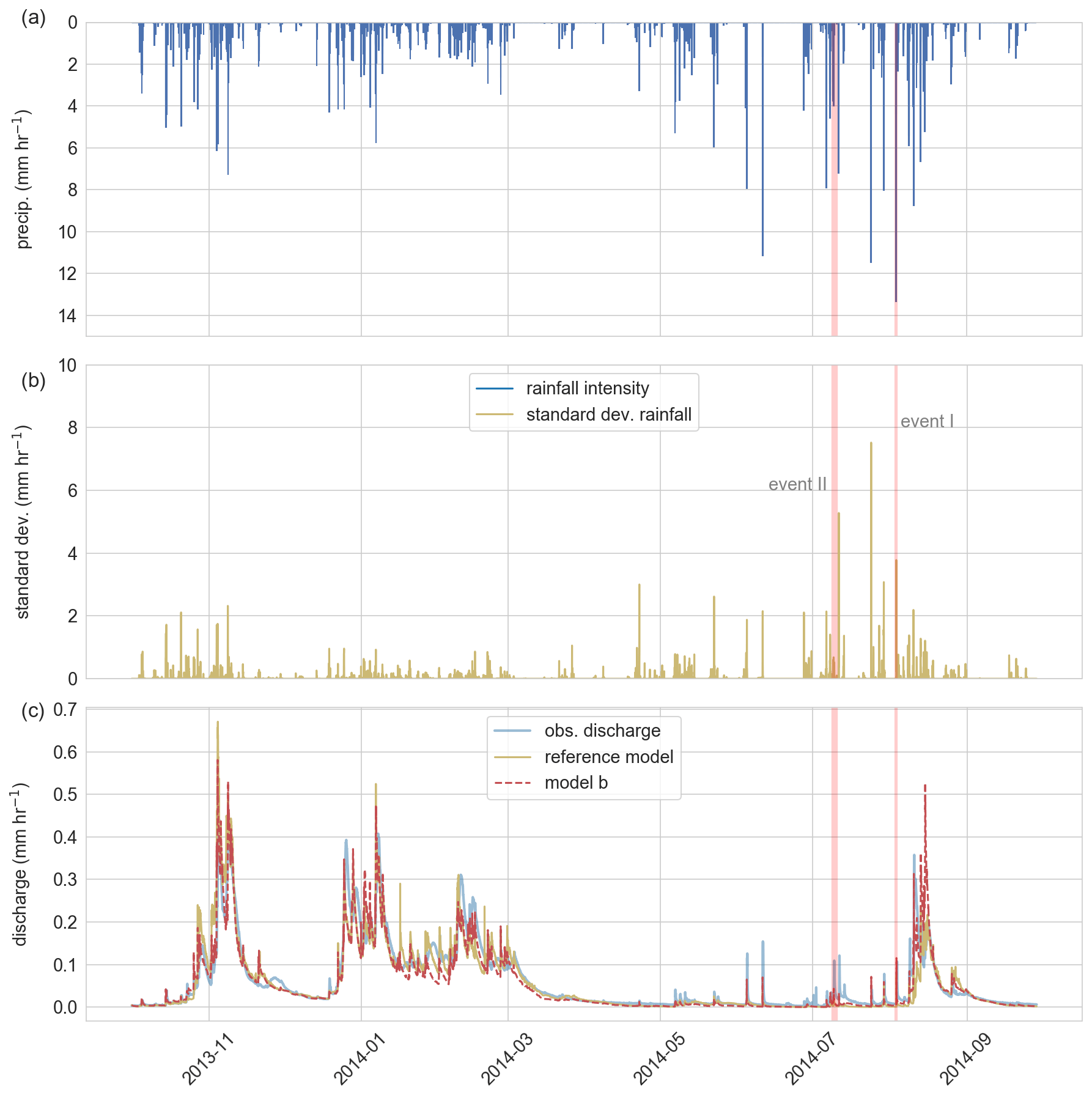
Figure 4(a) Average rainfall intensity of the precipitation field (mm h−1), (b) corresponding standard deviation of the precipitation field (mm h−1), (c) observed discharge of the Colpach catchment and the discharge simulation of the reference model as well as of the distributed model b. The two red bars display the location of the two selected rainfall-runoff events used to test the adaptive clustering approach.
We selected two rainfall-runoff events to test the adaptive model c (Fig. 4). We chose the first event as it has the highest rainfall intensity of 19 mm h−1 and the third-highest spatial variability estimated by the standard deviation of 3.8 mm h−1 in the time series as well as a distinct runoff reaction. Rainfall event I was observed at the beginning of August and lasted for about 5 h, and the highest spatial differences between the grid cells of 14 mm h−1 was reached right at the beginning of the event (Figs. 5 and 6). The rainfall event I moved from west to east over the catchment and reached its maximum rainfall intensity after 3 h. No rainfall had occurred before the event for a period of 102 h. It can hence be assumed that the catchment was in a moderately dry state before the event, also indicated by soil moisture measurements presented in Loritz et al. (2017).
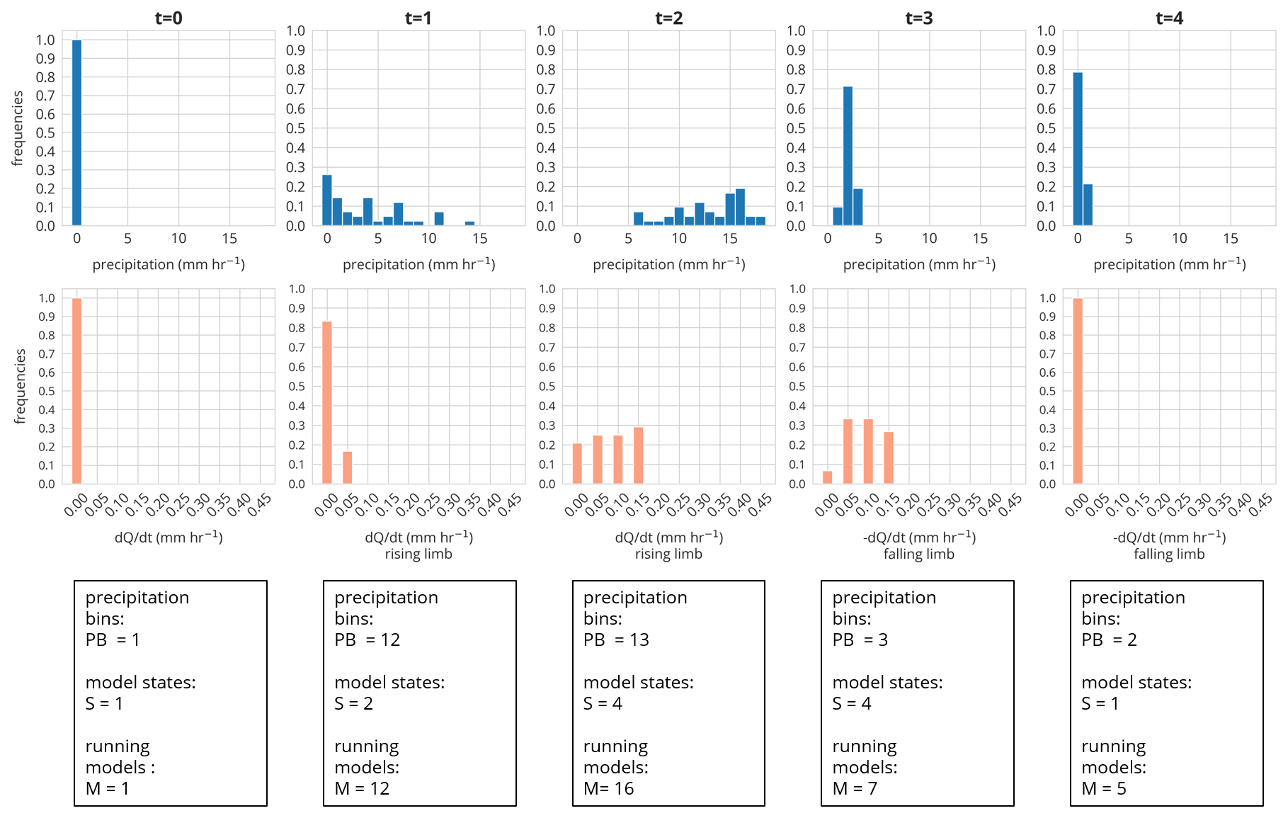
Figure 5Binned precipitation field (blue) and binned model states (orange) of the adaptive model (t=0; 3 August 2014 15:00 CET). PB is the no. of allocated precipitation bins, S the no. of allocated model space bins, and M the no. of running models at the given time step. The spatial distribution of the precipitation and the model states for event I are displayed in Fig. 6.
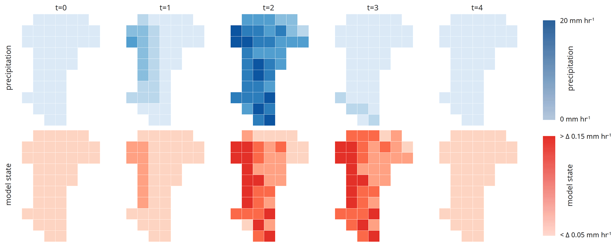
Figure 6Spatial and temporal distribution of the precipitation field (upper panel) and the corresponding states of the actual model grids used by the adaptive model c (lower panel). The model state is estimated by the slope of the simulated discharge. The corresponding bins (groups) of the precipitation and model states are shown in Fig. 5.
The second rainfall event was selected as it has distinctly different properties (low spatial variability, low intensity, longer duration) as compared to the first event. Event II has a maximum rainfall intensity of 5.8 mm h−1 and a maximum spatial difference between the grid cells of 4 mm h−1. The event lasted for around 15 h, making it the longest continuing rainfall in the summer season, and there was no rainfall observed 20 h before the event but more than 36 mm of rainfall over the preceding 3 d. It seems hence reasonable to assume that the soils in the catchment were rather wet, which is again supported by the soil moisture measurements presented in Loritz et al. (2017).
5.2 Temporal dependency of the model performance
The performances of the four model setups (reference model and model a, b, and c) to simulate the observed discharge of the Colpach catchment estimated by means of the KGE are shown in Table 2. Comparing the two spatially aggregated models that differ only with respect to their rainfall forcing, the reference model outperforms model a during the winter season and on the annual timescale, while model a has a higher performance during the vegetation season (April–September). Both models are characterized by KGE values higher than 0.8 in the winter season and for the entire hydrological year, while the predictive performance drops in summer and is particularly low for the two rainfall-runoff events, even resulting in negative KGE values. The differences between the KGE values (ΔKGE) between the two spatially aggregated models (reference model and model a) are low in winter, increase in summer, and are the highest for the convective rainfall event I. Here model a only has a slightly improved predictive performance as the average discharge of the event, indicated by a KGE value of −0.16 (please note that the performance of the mean of the observation is not zero as in the case when using the Nash–Sutcliffe efficiency, as shown by Knoben et al., 2019).
Table 2Model performances of the four model setups to simulate the observed discharge of the Colpach catchment measured using the Kling–Gupta efficiency (KGE), based on hourly simulation and observation time steps. Performances are shown for the entire hydrological year (2013/2014), for the winter (October–March) and summer season (April–September), and for two selected summer rainfall-runoff events in July and August. The three components of the KGE can be found in the Supplement.
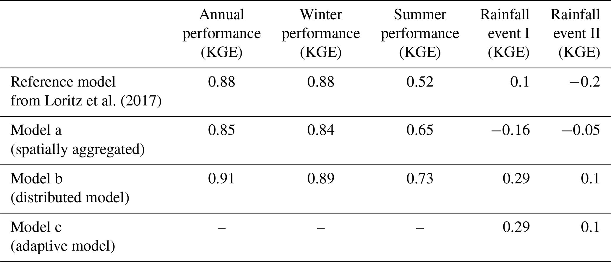
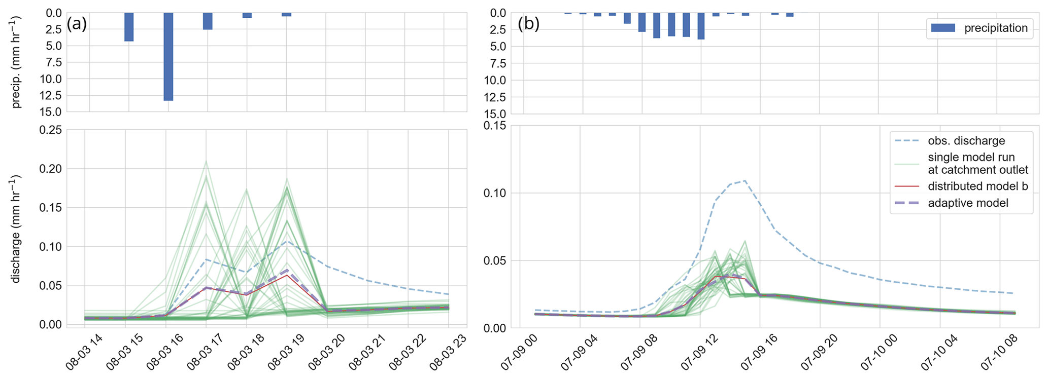
Figure 7(a) Rainfall-runoff event I and (b) rainfall-runoff event II. Blue bars in the upper panel show the average precipitation of the precipitation field for each time step (mm h−1). The green curves in the lower panel represent a single gridded model of the distributed model b, the red line the area-weighted mean of the distributed model, the dashed purple line the area-weighted mean of the adaptive model, and the dashed blue line the observed specific discharge of the Colpach.
The observed discharge of the Colpach catchment and the discharge simulations of the reference model, as well as the discharge simulation of the distributed model b, are presented in Fig. 4c. Visual comparison of the two models shows that the reference model has lower runoff production during summer, which is particularly visible in August and September. Interestingly, the latter cannot be explained by the annual or seasonal precipitation sums as both models are driven on average by similar precipitation sums of around 900 mm yr−1 for the entire year and around 450 mm per 6 months in the summer season. Overall, model b has the highest predictive performance as indicated by the KGE in all five test periods (annual, winter, summer, and the two selected rainfall events) when compared to the two spatially aggregated models (reference model and model a). The absolute differences between the model performances depend again on the selected period. For instance, for the entire simulation period, the reference model and model b have close to equal KGE values around 0.9, while the differences between the KGE values are ΔKGE = 0.21 in summer and for the rainfall event II around ΔKGE = 0.3.
Although model b has the highest KGE values for the two selected rainfall-runoff events, the general model performance is, given the KGE values of 0.29 and 0.1, still relatively low for both runoff events. The low performance can be explained by a general underestimation of the total runoff volume at both events (Fig. 7), while it seems that the shape of the simulated hydrograph is simulated acceptably underpinned by a correlation of 0.72 and 0.86 between the simulation and observation (see Supplement for the three components of the KGE). The latter is supported by the fact that distributed model b is able to simulate the observed double peak at event I. We furthermore tested the addition of a direct runoff component by assuming that 10 % of the rainfall is directly added to the channel network instead of falling on the hillslopes. This model extension could be justified by sealed areas within the catchment or by precipitation that directly falls into the stream or on saturated areas like the riparian zone. This rather simple model extension increases the KGE of model b from 0.29 to 0.48 at event I. However, we do not update our model here as the main goal of this study is not to perform the best possible rainfall-runoff simulation but to investigate the role of the spatiotemporal patterns of rainfall in the runoff generation of a mesoscale catchment by introducing the concept of a spatially adaptive hydrological model.
5.3 Spatially adaptive modeling – simulation results
The upper panel of Fig. 5 shows the binned precipitation field of rainfall event I. The precipitation field was binned based on the chosen bin width of 1 mm h−1. The rainfall field allocates 0 bins (precipitation groups) at t=0 (PB = 0), 12 bins at t=1 (PB = 12), 13 bins at t=2 (PB = 13), 3 bins at t=3 (PB = 3), and 2 bins at t=4 (PB = 2). The number of occupied bins indicates the spatial variability of the rainfall event at a given time step and would reach maximum spatial complexity if PB equals 42. This means that if a high number of bins is allocated, the forcing is spatially variable and therefore a higher number of models is needed to represent the spatial variability of the precipitation. The number of bins does, however, not specify how large the gradients are within the spatial precipitation field. For instance, if 50 % of a precipitation field is characterized by a rainfall amount of 20 mm h−1 and the other 50 % by 1 mm h−1, the number of allocated bins is two, although the absolute difference between the bins is large.
The lower panels of Figs. 5 and 6 display the binning of the model states (S) of the adaptive model for each time step of event I for the similarity measure dQ dt−1. We do not plot the similarity measure Q here as in our specific case, Q and dQ dt−1 lead to the same classification at both events. However, this does not mean that Q is less relevant as in theory two models could simulate identical dQ dt−1 values but very different absolute Q values. This shows that the set of similarity measures should be picked carefully and depend very much on the given modeling task and the research environment.
At t=0, we run a single model representing the entire catchment with a single model state. At t=1, the precipitation starts, and the spatial field is classified into 12 bins (PB = 12). Following our approach, this necessitates that we need to run 12 models (M=12) at t=1 to account for the spatial variability of the rainfall. After one simulation step, we estimate the number of model states by binning the absolute values (Q) and slope (dQ dt−1) of the discharge simulations of the 12 models, resulting in two different model states (two model state bins are occupied). Each of these states represents now a different part of the catchment with a different area (Fig. 6, lower panel). For instance, at t=1 around 76 % of the catchment area is represented by a model in a state where discharge changes below 0.05 mm h−1 and 14 % between 0.05 and 0.1 mm h−1. At t=2, the precipitation field has been classified into 13 bins, but at this time step, the catchment is represented by two model states from the time step before. This means we need to check which combinations of states and precipitation input occur, in other words, which grids are represented by which state and are forced by which precipitation input. In this specific setting, we need to run 16 models, which is lower than the theoretical maximum (2 model states S×13 precipitation bins (PB = maximum of 26 running models M) as not all model states are driven by all binned precipitation inputs. Afterward, we again group the model states (S=4) and continue until t=4 after which no rainfall occurs, and we again represent the entire catchment by a single hillslope model. In total, we were able to reduce the maximum number of gridded models from 42 to a maximum of 16 at rainfall event I and at the second event from 42 to 4 without a predictive performance loss in comparison to the distributed model b (Table 2). The latter is shown by the KGE values between the distributed model b and the adaptive model c of around 0.98 at both events.
5.4 Spatially adaptive modeling – dissipation of differences
The dissipation timescale (memory timescale) for both events until the different hillslope models have “forgotten” the last forcing and are again in the same “runoff generation state” is relatively short. Specifically, already after 1 h of no precipitation at event I and II, the difference between the hillslope models in model c is below the selected threshold of 0.05 mm h−1 for Q and dQ dt−1. The same is true for the soil moisture distributions at 10–20 and 60–100 cm depth, which is negligibly small at the time step t=4 at event I when the four hillslope models are aggregated. This means that the entire catchment can again be represented by a single hillslope model already shortly after the last rainfall at both events until new rainfall (PB > 1) occurs. The latter is supported as the single hillslope from model c and the spatially aggregated model a are also in a similar state regarding their runoff generation after t=5 at event.
This picture might, however, be different in certain simulation scenarios. For instance, Fig. 8 displays the soil moisture distribution of two hillslope models at 10–20 and 60–100 cm depth at three time steps during event I (t=3, t=24, and t=48) that either have received the highest amount of rainfall measured at a grid cell (30 mm, 5 h−1) or the lowest (15 mm, 5 h−1). Both hillslope models started in the same initial model state, and the dissipation time of the topsoil correlates well with the runoff generation. The largest deviation between the “wettest” model, which has received the highest amount of rainfall, and the “driest” model, which has received the lowest amount of rainfall, is at t=3 shortly after the highest rainfall intensity (see Fig. 5). After 24 h, this difference persists but slowly dissipates and has almost completely disappeared after 48 h. In the deeper soil layer, the picture is different. During the event, we see no reaction to the rainfall forcing in the deeper soil layers. However, 24 h after the first rainfall, the two models deviate also in deeper layers, and the deviation is in a similar range as in the top soil, although there was no further rainfall. The difference in both layers disappears again after 48 h of no rainfall, and the wettest and driest model are again in a similar state, also regarding their soil moisture distributions.
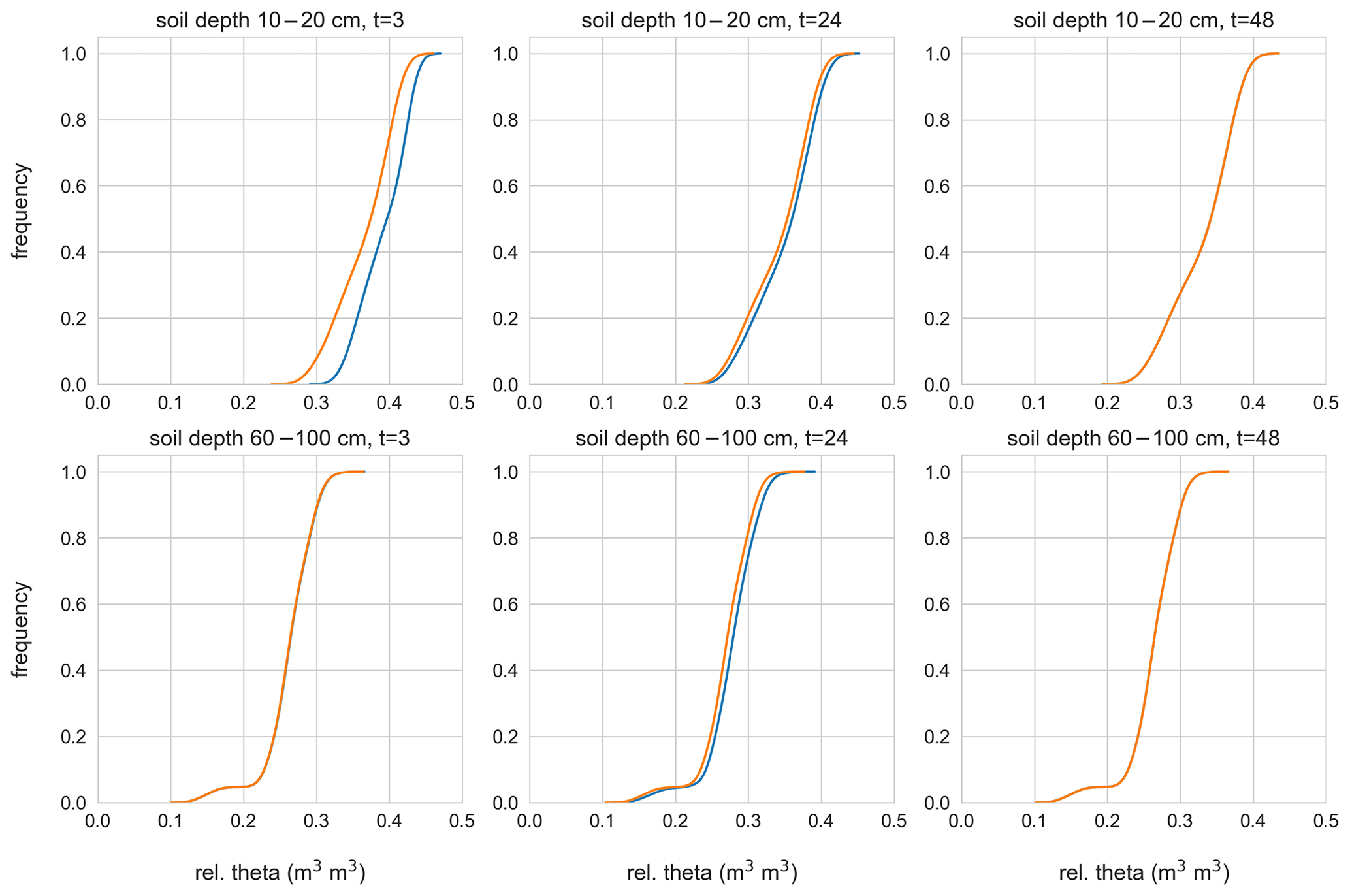
Figure 8Relative soil moisture distributions for two gridded hillslope models that received the lowest (orange curve) and the highest (blue curve) amount of rainfall during event I (15 mm 5 h−1 and 30 mm 5 h−1). Presented for time step t=3 (during the event), t=24 (after the event), and t=48 (after the event).
6.1 The role and value of distributed rainfall in hydrological models
While the three non-adaptive model setups (reference model, model a, and b) perform equally well simulating the discharge of the Colpach catchment in the winter season, this is not the case in the summer season, when the distributed model b has higher KGE values than both spatially aggregated models. This corroborates one of our hypotheses stating that the predictive performance of the representative hillslope (reference model) introduced by Loritz et al. (2017) increases if the model is distributed in space and driven by distributed rainfall. Nevertheless, model b still has several deficiencies, especially for the two selected rainfall events when it does underestimate the total observed runoff volume, resulting in high correlation values but overall low KGE values. The latter shows that there is potential to improve the predictive performance of the model beyond only changing the precipitation input, for instance by accounting for the sealed areas and forest roads in the catchment.
Although the model comparison in this study is rather heuristic (e.g., we discuss mainly along a single integrating performance metric), the findings in this study show that the use of distributed rainfall is at least recommended during the summer season in this catchment. This contradicts the results of, for instance, Obled et al. (1994), who argued that the precipitation over a 71 km2 large catchment is not sufficiently organized to be relevant for the runoff generation. It is also not in line with the findings of Nicótina et al. (2008), who recommended the use of distributed rainfall only in specific scenarios (e.g., infiltration excess) or in catchments above 8000 km2. Given the improved performance of the distributed model b and the rather small size of the Colpach catchment of less than 20 km2, it seems reasonable to conclude that catchment size alone might not be the best indicator to decide if a distributed hydrological model driven by distributed rainfall is needed or not.
As the dominant rainfall generation mechanisms change during the hydrological year in many catchments from frontal to convective, it does not come, from a physical perspective, as a surprise that the increased relevance of distributed rainfall in summer can be linked to the changing meteorological properties. Ogden and Julien (1993) argued along these lines when they showed that the spatial distribution of rainfall is only a dominant control in the case that rainfall events have a shorter duration than the average runoff concentration time of a catchment. Similarly, Zhu et al. (2018) reasoned that the spatial patterns of precipitation are less relevant compared to the temporal distribution if the drainage area and therefore typically the concentration time is decreasing. The question as to whether a structurally similar catchment needs to be represented in a spatially distributed manner depends hence on the spatial and temporal structure of the precipitation as well as on the average concentration time as a first proxy for the catchment size.
The changing model performances during the two events highlight that the required model and precipitation resolution does not only change between seasons but can vary from rainfall event to rainfall event. This has also been argued by Watts and Calver (1991), who stated that “the finest available definition of rainfall may be desirable for modeling …” of convective rainfall events, while lower spatial model resolutions are sufficient during spatially and temporal more homogenous often stratiform rainfall events. In contrast, Lobligeois et al. (2014) reported that the distribution of rainfall is in general of higher relevance in certain regions of France when they analyzed 3620 rainfall-runoff events in 181 different mesoscale catchments. However, they also argued that a substantial number of rainfall-runoff events do not match this general pattern, showing that the distribution of rainfall can be of high importance, even if the spatial precipitation patterns are usually not a dominant control on the runoff formation in a region. As such “rare” events are frequently linked to extremes that are in turn beyond the realms of experience of what these landscapes have adapted to, they are of considerable importance despite their low occurrence in time (e.g., Loritz, 2019). This point is underpinned by the work of Zhu et al. (2018) and Peleg et al. (2017), who both questioned the common practice to use spatially uniform rainfall based on a single or a few rain gauges for performing flood risk assessments, especially for higher return periods in rural and urban catchments, respectively. The proposed spatially adaptive modeling approach could thereby be one way to tackle this issue as it enables continuous physically based simulations with model structures that adapt to the precipitation forcing.
6.2 Spatially adaptive modeling – as a tool to reduce redundant computations
The first results of the adaptive modeling approach seem promising as the spatial adaptive model c performed similarly as the distributed model b, however, using a smaller number of hillslopes. Similar findings were reported, for instance, by Chaney et al. (2016). They applied their HRU-based model called “HydroBlocks” in a 610 km2 large catchment and showed that a compressed, semi-distributed model consisting of 1000 HRUs performed similarly compared to a gridded fully distributed model while being 2 orders of magnitude faster than the distributed model and requiring only 0.5 GB instead of 250. They concluded that “… the spatial patterns of the fully distributed model can be reproduced with a fraction of the computational expense”, highlighting the potential of approaches like HydroBlocks as tools to improve the representation of hydrological processes in large-scale land surface models without drastically increasing the computational times and model complexity.
The main difference between models like HydroBlocks and our approach is that HRUs are dynamically reassigned during model execution based on the spatial properties of the precipitation forcing. By that, we try to avoid redundant calculations to reduce computational times similar to Chaney et al. (2016) but also try to avoid situations in which we underestimate the spatial variability of the meteorological forcing or the system state in the case that the test period is not representative for certain spatial constellations. The latter can thereby significantly impact hydrological simulations during extreme conditions (e.g., Zehe et al., 2005; Zhu et al., 2018). Our results show that the maximum number of gridded models necessary to represent the variability of the catchment states and precipitation elements can be reduced by a factor of 2.5. The total gain in computational efficiency is however larger as the majority of the time, fewer than 16 models are required to represent the catchments' runoff generation. For instance, during low flow conditions the spatially aggregated model a, all hillslopes of the spatially distributed model b, and the spatially adaptive model c are in a similar state and hence produce similar results. In addition, the fact that during the winter season a single representative hillslope (reference models) performs close to similarly to the distributed model b indicates that the possibility to save computational times by dynamically adapting the model structure is higher than the factor of 2.5 suggests.
Clark et al. (2017) recognized computational times as a major obstacle when using physically based models for practical applications, as proposed in the landmark publication of Freeze and Harlan (1969). The discussion about saving computational times with adaptive clustering is, however, challenging as the gain depends on the model approach chosen (e.g., numerical scheme), the hardware used, the programming language, the compiler, or the number of printout times to the hard drive (Ehret et al., 2020). The relevance of saving computational times of, for instance, 10 % depends furthermore on the absolute calculation time of a model and whether a model run needs 100 min or 100 d to be completed. A fair comparison would mean setting up a virtual environment and working under similar conditions, e.g., using a virtual machine as well as using a fully automated adaptive clustering approach and running the adaptive model c on longer timescales, at which it will most likely be the most useful. Both are, however, beyond the scope of this study, and we point toward the study of Ehret et al. (2020), which discusses the potential of adaptive clustering with respect to saving computational times in detail.
6.3 Spatially adaptive modeling – as a learning tool to better understand the dissipative nature of a hydrology
In this study, we focus on the potential of adaptive modeling to examine when interactions between a variable precipitation forcing and a variable catchment state cause a variable runoff response and when these differences get “forgotten” due to the dissipative nature of hydrological systems. Our results illustrate that the relevance of distributed rainfall for hydrological modeling is dynamically changing in space and time. One way to account for this dynamically changing importance is to run distributed models driven by distributed rainfall the entire time at the highest possible resolution. Such an approach would avoid cases in which we unnecessarily underestimate the needed (spatial) model complexity of a hydrological model, which again could lead to limited predictive performances (e.g., Fenicia et al., 2011; Höge et al., 2019; Schoups et al., 2008). However, this procedure may result in a strong increase of uncertainty due to an increased number of model parameters (e.g., Beven, 1989), frequently by an unchanged amount of data for validation (Melsen et al., 2016), lead to a general overestimation of the simulated spatial variability due to error propagations and can drastically increase the number of redundant computations (Clark et al., 2017; Loritz et al., 2018). The issue of increasing computational times due to redundant calculations is thereby reinforced by the fact that physically based simulations of hydrological fluxes rely on relatively short natural length scales in time and space. For instance, the water flow in the critical zone, which is frequently simulated using the Darcy–Richards equation, should not exceed a lateral grid size of 10 m and a vertical grid size below 1 m in homogeneous soils (Vogel and Ippisch, 2008). The same is true, although on other scales, for simulating surface runoff with derivatives of the Saint-Venant equation but also for conceptual models for which the assumption that a few macroscopic water tables can represent the heterogeneity of driving potentials in a landscape is rarely questioned. Even the gridded spatial resolution of 100 m proposed in the comment by Wood et al. (2011) for hyper-resolution models seems from a purely physical perspective on hydrological processes questionable given the importance of hillslopes as key building blocks in a hydrological landscape (Fan et al., 2019). This is underpinned by the fact that hillslopes in the upper part of the Colpach are barely longer than 100 m, but different segments of these hillslopes can vary substantially in their wetness and connections to the river (e.g., Martínez-Carreras et al., 2016). Hydrological physically based modeling with top-down or bottom-up models without a delineation of the underlying system in smaller sub-units is hence up-to-date constrained to rather short length scales, at least if applications do not compromise the underlying physics.
Physical constraints, which result in small grid sizes and calculation time steps, must however not be a dead-end for physically based modeling on larger scales. This is because it is frequently found that different catchments in the same hydrological landscape function similarly despite the overwhelming small-scale variability we frequently observe on the plot scale (e.g., Mälicke et al., 2020; Sternagel et al., 2019). This phenomenon sometimes referred to as spatial organization entails a large potential for hydrological modeling as it allows information about functional relationships and catchment states to be transferred from one catchment to another (e.g., Hrachowitz et al., 2013) as well as offering the possibility to aggregate structurally similar sub-units and simulate their function by a representative model element (e.g., Sivapalan et al., 1987; Zehe et al., 2014). The fact that hydrological systems are highly dissipative (Loritz et al., 2019) but constrained by their structural setting is thereby the key to explain the feasibility of this aggregation as the unique characteristics of the forcing over an area do not prevail but are depleted or “forgotten” in a relatively short time, at least if the focus is on the runoff generation. Specifically, we found during both tested events that already after 1 h of no rainfall the spatially adaptive model c required only a single hillslope model to represent the runoff generation of the Colpach. While this finding is surely constrained by the chosen thresholds of the two selected similar metrics (dQ dt−1 and Q) and the chosen time frame, the picture is underpinned by the soil moisture distributions of the model elements of the spatially adaptive model c that are also close to similar at the time step when they are aggregated.
Nonetheless, another virtual experiment showed that there are clear limitations to the proposed approach and the chosen parameters. We could demonstrate that two hillslope models that received significant dissimilar precipitation amounts (>15 mm 5 h−1) showed differences regarding their soil moisture distributions in 60–100 cm 24 h after the last rainfall, although the runoff generation at this time step was close to similar. The latter means that there could be specific circumstances when we aggregate hillslope models using the chosen similarity measures dQ dt−1 and Q and thereby remove relevant information about the different model states from our ensemble. This is the case as we can simulate the same flux by combining different combinations of driving potentials with integral resistance terms, a phenomenon that is inherent to all our governing equations and sometimes referred to as equifinality in hydrological modeling (Beven, 1993; Loritz et al., 2019; Zehe et al., 2014). This highlights that the similarity metrics that are used to group similar models by their state should be chosen with care and need to be adapted to the given research environment and process under study. For instance, in a snow-dominated area we need to group model states not only based on their runoff production but also based on their snow cover. The choice of dQ dt−1 and Q in this study seems, however, to be sufficient to identify similar model elements, at least as long as we focus on the summer season. This is the case as our hillslope models are all structurally identical and only simulate shallow subsurface storm flow during the entire summer season. We can hence assume that we do have a rather unique relationship between our model states and the chosen similarity metrics dQ dt−1 and Q. This is underpinned by the fact that the individual hillslope models of the distributed model b, which reflect the highest spatial resolution of the spatially adaptive model c, do not drift apart in the chosen summer season. Conversely, they mainly produce redundant simulations already shortly after each rainfall event, at least as long as we focus on the summer season (see Supplement). The latter means, however, also that the conclusions drawn are not necessarily true for the winter season for which we have not tested the adaptive model as the distributed model b and spatially aggregated reference model perform close to similarly. Nevertheless, a test of the proposed spatially adaptive modeling approach on a longer timescale is an interesting task for further research.
While the structure of a catchment constraints its state space, its actual position therein is controlled by the meteorological forcing and by an attracting local thermodynamic equilibrium, a point where all driving gradients are depleted. As larger gradients dissipate faster than smaller ones, as long as they are controlled by the same integral resistance properties, structurally similar parts of a landscape will converge to the same state and thereby “forget” differences between their past forcing and current state. This convergence leads to the emergence of hydrological similarity in time (Loritz et al., 2018) and explains the changing relevance of distributed rainfall within hydrological models. This again is the theoretical foundation that explains why adaptive modeling works in hydrological systems and not necessarily in meteorological systems as their chaotic nature can amplify state differences on longer timescales, instead of dissipating those (e.g., Lorenz, 1963). Our developed adaptive modeling approach uses this straightforward physical reasoning of the causal and dissipative interplay between the precipitation forcing and the catchment state to dynamically allocate its model structure during model execution. It is built upon a well-established concept in hydrology, which assumes that individual observations or model states can represent each other if they are allocated to the same group (e.g., Wood et al., 1990). The related bin widths (grouping) can be selected either based on our physical understanding (Loritz et al., 2018) or identified based on a statistical analysis of the underlying distribution (of for instance the precipitation data; e.g., Gong et al., 2014; Scott, 1979). The general approach is strongly motivated by the idea that a spatially homogeneous field can be compressed to a single time series without losing information about the spatial pattern of rainfall. This is, however, not the case if the spatial field is highly variable, where a compression to a single observation reduces the information provided to a hydrological model and hence can average out extremes and potentially relevant spatial constellations (e.g., Loritz et al., 2018; Weijs et al., 2013). Spatially adaptive modeling can, therefore, be used not only as a tool to reduce computational times but also to analyze the relevance of certain spatial detail in a hydrological model and therefore as a tool to better understand the dissipative nature of hydrology.
In this study, we investigate the role and value of distributed precipitation data in the runoff generation of a mesoscale catchment. We therefore compare the model performances of four model setups at different periods and show that a distributed model driven by distributed rainfall yields improved performances only during certain periods. We then step beyond this finding and develop a spatially adaptive model that is able to dynamically adjust its spatial model structure in time. This model is capable of representing the varying importance of distributed rainfall within a hydrological model without losing predictive performance compared to a spatially distributed, gridded model. Our results confirm that spatially adaptive modeling might be one way to reduce computational times in physically based hydrological simulations as well as being used as a tool to better understand the causal and dissipative interplay between a catchment's state and its meteorological forcing.
The main findings of this study are as follows:
-
The importance of distributed rainfall in hydrological modeling is given by the natural variability of rainfall dynamically changing in time. In consequence, there cannot be a time-invariant answer to the question – “how important are spatial patterns of precipitation for the runoff generation at the catchment scale?” – nor to any related question which deals with an “optimal” spatial discretization of a hydrological landscape within a model.
-
Spatially adaptive modeling is a feasible way to account for the changing importance of distributed rainfall within a hydrological model and at the same time can be used as a tool to improve our understanding of the interplay between rainfall forcing, catchment structure, and its state.
-
Hydrological landscapes are organized in a manner that spatial differences within the precipitation forcing are “forgotten” or smoothed out in often surprisingly short period when rainfall becomes runoff. This means that gradients that drive runoff are effectively dissipated, which happens frequently under the influence of various forms of preferential flow (e.g., Berkowitz and Zehe, 2020). The dissipative nature of hydrological processes combined with the observation that structural similar hydrological landscapes are also functionally organized similarly explains thereby why hydrological similarity must be a time-invariant concept and why spatially adaptive modeling is a physically reasonable way to represent hydrological systems within a model.
The hydrological model CATFLOW and all simulation results are available from the lead author on request. The rainfall data are available from Malte Neuper on request. The discharge observations were provided by the Luxembourg Institute of Science and Technology and are available from Laurent Pfister on request.
The supplement related to this article is available online at: https://doi.org/10.5194/hess-25-147-2021-supplement.
RL wrote the paper, had the main idea for the adaptive modeling, and carried out all analysis and model simulations. EZ and MH helped significantly with interpreting the results, with setting up the models, and with the editing. MN provided quality-controlled rainfall data for the analysis and provided assistance with his meteorological expertise.
The authors declare that they have no conflict of interest.
This research contributes to the Catchments As Organized Systems (CAOS) research group (FOR 1598), funded by the German Science Foundation (DFG ZE 533/11-1, ZE 533/12-1). Laurent Pfister and Jean-Francois Iffly from the Luxembourg Institute of Science and Technology (LIST) are acknowledged for organizing the permissions for the experiments and providing discharge data and the digital elevation model. Finally, we thank the editor Nadav Peleg and the four referees listed in alphabetical order, Wouter Knoben, Hannes Müller-Thomy, Anna E. Sikorska-Senoner, and Daniel Wright, for their critical but very constructive comments.
The article processing charges for this open-access publication were covered by a Research Centre of the
Helmholtz Association.
This paper was edited by Nadav Peleg and reviewed by Daniel Wright, Wouter Knoben, Hannes Müller-Thomy, and Anna E. Sikorska-Senoner.
Berger, M. J. and Oliger, J.: Adaptive mesh refinement for hyperbolic partial differential equations, J. Comput. Phys., 53, 484–512, https://doi.org/10.1016/0021-9991(84)90073-1, 1984.
Berkowitz, B. and Zehe, E.: Surface water and groundwater: Unifying conceptualization and quantification of the two “water worlds”, Hydrol. Earth Syst. Sci., 24, 1831–1858, https://doi.org/10.5194/hess-24-1831-2020, 2020.
Beven, K.: Changing ideas in hydrology – The case of physically-based models, J. Hydrol., 105, 157–172, https://doi.org/10.1016/0022-1694(89)90101-7, 1989.
Beven, K.: Prophecy, reality and uncertainty in distributed hydrological modelling, Adv. Water Resour., 16, 41–51, https://doi.org/10.1016/0309-1708(93)90028-E, 1993.
Beven, K.: Dalton Lecture: How Far Can We Go In Distributed Hydrological Modelling?, Lancaster University, Long Beach, California, 1–12, available at: http://eprints.lancs.ac.uk/4420/ (last access: 15 June 2020), 2001.
Beven, K. and Binley, A.: The future of distributed models: Model calibration and uncertainty prediction, Hydrol. Process., 6, 279–298, https://doi.org/10.1002/hyp.3360060305, 1992.
Beven, K. and Freer, J.: A dynamic topmodel, Hydrol. Process., 15, 1993–2011, https://doi.org/10.1002/hyp.252, 2001.
Beven, K. J. and Hornberger, G. M.: Assessing the effect of spatial pattern of precipitation in modeling stream flow hydrographs, J. Am. Water Resour. Assoc., 18, 823–829, https://doi.org/10.1111/j.1752-1688.1982.tb00078.x, 1982.
Celia, M. A., Bouloutas, E. T., and Zarba, R. L.: A general mass-conservative numerical solution for the unsaturated flow equation, Water Resour. Res., 26, 1483–1496, https://doi.org/10.1029/WR026i007p01483, 1990.
Chaney, N. W., Metcalfe, P., and Wood, E. F.: HydroBlocks: a field-scale resolving land surface model for application over continental extents, Hydrol. Process., 30, 3543–3559, https://doi.org/10.1002/hyp.10891, 2016.
Clark, M. P., Bierkens, M. F. P., Samaniego, L., Woods, R. A., Uijlenhoet, R., Bennett, K. E., Pauwels, V. R. N., Cai, X., Wood, A. W., and Peters-Lidard, C. D.: The evolution of process-based hydrologic models: historical challenges and the collective quest for physical realism, Hydrol. Earth Syst. Sci., 21, 3427–3440, https://doi.org/10.5194/hess-21-3427-2017, 2017.
Das, T., Bárdossy, A., Zehe, E., and He, Y.: Comparison of conceptual model performance using different representations of spatial variability, J. Hydrol., 356, 106–118, https://doi.org/10.1016/j.jhydrol.2008.04.008, 2008.
Ehret, U., van Pruijssen, R., Bortoli, M., Loritz, R., Azmi, E., and Zehe, E.: Adaptive clustering: reducing the computational costs of distributed (hydrological) modelling by exploiting time-variable similarity among model elements, Hydrol. Earth Syst. Sci., 24, 4389–4411, https://doi.org/10.5194/hess-24-4389-2020, 2020.
Euser, T., Hrachowitz, M., Winsemius, H. C., and Savenije, H. H. G.: The effect of forcing and landscape distribution on performance and consistency of model structures, Hydrol. Process., 29, 3727–3743, https://doi.org/10.1002/hyp.10445, 2015.
Fan, Y., Clark, M., Lawrence, D. M., Swenson, S., Band, L. E., Brantley, S. L., Brooks, P. D., Dietrich, W. E., Flores, A., Grant, G., Kirchner, J. W., Mackay, D. S., McDonnell, J. J., Milly, P. C. D., Sullivan, P. L., Tague, C., Ajami, H., Chaney, N., Hartmann, A., Hazenberg, P., McNamara, J., Pelletier, J., Perket, J., Rouholahnejad-Freund, E., Wagener, T., Zeng, X., Beighley, E., Buzan, J., Huang, M., Livneh, B., Mohanty, B. P., Nijssen, B., Safeeq, M., Shen, C., Verseveld, W., Volk, J., and Yamazaki, D.: Hillslope Hydrology in Global Change Research and Earth System Modeling, Water Resour. Res., 55, 1737–1772, https://doi.org/10.1029/2018WR023903, 2019.
Fenicia, F., Kavetski, D., and Savenije, H. H. G.: Elements of a flexible approach for conceptual hydrological modeling: 1. Motivation and theoretical development, Water Resour. Res., 47, 1–13, https://doi.org/10.1029/2010WR010174, 2011.
Fenicia, F., Kavetski, D., Savenije, H. H. G., and Pfister, L.: From spatially variable streamflow to distributed hydrological models: Analysis of key modeling decisions, Water Resour. Res., 52, 954–989, https://doi.org/10.1002/2015WR017398, 2016.
Freeze, R. A. and Harlan, R. L.: Blueprint for a physically-based, digitally-simulated hydrologic response model, J. Hydrol., 9, 237–258, https://doi.org/10.1016/0022-1694(69)90020-1, 1969.
Gong, W., Yang, D., Gupta, H. V., and Nearing, G.: Estimating information entropy for hydrological data: One-dimensional case, Water Resour. Res., 50, 5003–5018, https://doi.org/10.1002/2014WR015874, 2014.
Hannesen: Analyse konvektiver Niederschlagssysteme mit einem C-Band Dopplerradar in orographisch gegliedertem Gelände, University of Karlsruhe, Karlsruhe, 1998.
Höge, M., Guthke, A., and Nowak, W.: The hydrologist's guide to Bayesian model selection, averaging and combination, J. Hydrol., 572, 96–107, https://doi.org/10.1016/j.jhydrol.2019.01.072, 2019.
Hopp, L. and McDonnell, J. J.: Connectivity at the hillslope scale: Identifying interactions between storm size, bedrock permeability, slope angle and soil depth, J. Hydrol., 376, 378–391, https://doi.org/10.1016/j.jhydrol.2009.07.047, 2009.
Hrachowitz, M. and Clark, M. P.: HESS Opinions: The complementary merits of competing modelling philosophies in hydrology, Hydrol. Earth Syst. Sci., 21, 3953–3973, https://doi.org/10.5194/hess-21-3953-2017, 2017.
Hrachowitz, M. and Weiler, M.: Uncertainty of Precipitation Estimates Caused by Sparse Gauging Networks in a Small, Mountainous Watershed, J. Hydrol. Eng., 16, 460–471, https://doi.org/10.1061/(ASCE)HE.1943-5584.0000331, 2011.
Hrachowitz, M., Savenije, H. H. G., Blöschl, G., McDonnell, J. J., Sivapalan, M., Pomeroy, J. W., Arheimer, B., Blume, T., Clark, M. P., Ehret, U., Fenicia, F., Freer, J. E., Gelfan, a., Gupta, H. V., Hughes, D. A., Hut, R. W., Montanari, A., Pande, S., Tetzlaff, D., Troch, P. A., Uhlenbrook, S., Wagener, T., Winsemius, H. C., Woods, R. A., Zehe, E., and Cudennec, C.: A decade of Predictions in Ungauged Basins (PUB) – a review, Hydrolog. Sci. J., 58, 1198–1255, https://doi.org/10.1080/02626667.2013.803183, 2013.
Huang, Y., Bárdossy, A., and Zhang, K.: Sensitivity of hydrological models to temporal and spatial resolutions of rainfall data, Hydrol. Earth Syst. Sci., 23, 2647–2663, https://doi.org/10.5194/hess-23-2647-2019, 2019.
Jackisch, C.: Linking structure and functioning of hydrological systems, KIT – Karlsruher Institut of Technology, Karlsruhe, 2015.
Jackisch, C., Angermann, L., Allroggen, N., Sprenger, M., Blume, T., Tronicke, J., and Zehe, E.: Form and function in hillslope hydrology: in situ imaging and characterization of flow relevant structures, Hydrol. Earth Syst. Sci., 21, 3749–3775, https://doi.org/10.5194/hess-21-3749-2017, 2017.
Juilleret, J., Iffly, J. F., Pfister, L., and Hissler, C.: Remarkable Pleistocene periglacial slope deposits in Luxembourg (Oesling): pedological implication and geosite potential, Bull. la Société des Nat. Luxemb., 112, 125–130, 2011.
Kling, H. and Gupta, H.: On the development of regionalization relationships for lumped watershed models: The impact of ignoring sub-basin scale variability, J. Hydrol., 373, 337–351, https://doi.org/10.1016/j.jhydrol.2009.04.031, 2009.
Knoben, W. J. M., Freer, J. E., and Woods, R. A.: Technical note: Inherent benchmark or not? Comparing Nash–Sutcliffe and Kling–Gupta efficiency scores, Hydrol. Earth Syst. Sci., 23, 4323–4331, https://doi.org/10.5194/hess-23-4323-2019, 2019.
Leopold, L. B.: Downstream change of velocity in rivers, Am. J. Sci., 251, 606–624, https://doi.org/10.2475/ajs.251.8.606, 1953.
Lobligeois, F., Andréassian, V., Perrin, C., Tabary, P., and Loumagne, C.: When does higher spatial resolution rainfall information improve streamflow simulation? An evaluation using 3620 flood events, Hydrol. Earth Syst. Sci., 18, 575–594, https://doi.org/10.5194/hess-18-575-2014, 2014.
Lorenz, E. N.: Deterministic Nonperiodic Flow, J. Atmos. Sci., 20, 130–141, https://doi.org/10.1175/1520-0469(1963)020<0130:DNF>2.0.CO;2, 1963.
Loritz, R.: The role of energy and information in hydrological modeling, KIT – Karlsruhe Institute of Technology, Karlsruhe, 2019.
Loritz, R., Hassler, S. K., Jackisch, C., Allroggen, N., van Schaik, L., Wienhöfer, J., and Zehe, E.: Picturing and modeling catchments by representative hillslopes, Hydrol. Earth Syst. Sci., 21, 1225–1249, https://doi.org/10.5194/hess-21-1225-2017, 2017.
Loritz, R., Gupta, H., Jackisch, C., Westhoff, M., Kleidon, A., Ehret, U., and Zehe, E.: On the dynamic nature of hydrological similarity, Hydrol. Earth Syst. Sci., 22, 3663–3684, https://doi.org/10.5194/hess-22-3663-2018, 2018.
Loritz, R., Kleidon, A., Jackisch, C., Westhoff, M., Ehret, U., Gupta, H., and Zehe, E.: A topographic index explaining hydrological similarity by accounting for the joint controls of runoff formation, Hydrol. Earth Syst. Sci., 23, 3807–3821, https://doi.org/10.5194/hess-23-3807-2019, 2019.
Mälicke, M., Hassler, S. K., Blume, T., Weiler, M., and Zehe, E.: Soil moisture: variable in space but redundant in time, Hydrol. Earth Syst. Sci., 24, 2633–2653, https://doi.org/10.5194/hess-24-2633-2020, 2020.
Martínez-Carreras, N., Hissler, C., Gourdol, L., Klaus, J., Juilleret, J., François Iffly, J., and Pfister, L.: Storage controls on the generation of double peak hydrographs in a forested headwater catchment, J. Hydrol., 543, 255–269, https://doi.org/10.1016/j.jhydrol.2016.10.004, 2016.
Maurer, T.: Physikalisch begründete zeitkontinuierliche Modellierung des Wassertransports in kleinen ländlichen Einzugsgebieten, Karlsruher Institut für Technologie, Karlsruhe, 1997.
Melsen, L. A., Teuling, A. J., Torfs, P. J. J. F., Uijlenhoet, R., Mizukami, N., and Clark, M. P.: HESS Opinions: The need for process-based evaluation of large-domain hyper-resolution models, Hydrol. Earth Syst. Sci., 20, 1069–1079, https://doi.org/10.5194/hess-20-1069-2016, 2016.
Minkoff, S. E. and Kridler, N. M.: A comparison of adaptive time stepping methods for coupled flow and deformation modeling, Appl. Math. Model., 30, 993–1009, https://doi.org/10.1016/j.apm.2005.08.002, 2006.
Neuper, M. and Ehret, U.: Quantitative precipitation estimation with weather radar using a data- and information-based approach, Hydrol. Earth Syst. Sci., 23, 3711–3733, https://doi.org/10.5194/hess-23-3711-2019, 2019.
Nicótina, L., Alessi Celegon, E., Rinaldo, A., and Marani, M.: On the impact of rainfall patterns on the hydrologic response, Water Resour. Res., 44, 1–14, https://doi.org/10.1029/2007WR006654, 2008.
Obled, C., Wendling, J., and Beven, K.: The sensitivity of hydrological models to spatial rainfall patterns: an evaluation using observed data, J. Hydrol., 159, 305–333, https://doi.org/10.1016/0022-1694(94)90263-1, 1994.
Ogden, F. L. and Julien, P. Y.: Runoff sensitivity to temporal and spatial rainfall variability at runoff plane and small basin scales, Water Resour. Res., 29, 2589–2597, https://doi.org/10.1029/93WR00924, 1993.
Or, D., Lehmann, P., and Assouline, S.: Natural length scales define the range of applicability of the Richards equation for capillary flows, Water Resour. Res., 51, 7130–7144, https://doi.org/10.1002/2015WR017034, 2015.
Peleg, N., Blumensaat, F., Molnar, P., Fatichi, S., and Burlando, P.: Partitioning the impacts of spatial and climatological rainfall variability in urban drainage modeling, Hydrol. Earth Syst. Sci., 21, 1559–1572, https://doi.org/10.5194/hess-21-1559-2017, 2017.
Pfister, L., Martínez-Carreras, N., Hissler, C., Klaus, J., Carrer, G. E., Stewart, M. K., and McDonnell, J. J.: Recent Trends in Rainfall-Runoff Characteristics in the Alzette River Basin, Luxembourg, Hydrol. Process., 31, 1828–1845, https://doi.org/10.1023/A:1005567808533, 2017.
Pfister, L., Hissler, C., Iffly, J. F., Coenders, M., Teuling, R., Arens, A., and Cammeraat, L. H.: Contrasting Hydrologic Response in the Cuesta Landscapes of Luxembourg, in: The Luxembourg Gutland Landscape, edited by: Kooijman, A. M., Cammeraat, L. H., and Seijmonsbergen, A. C., Springer International Publishing, Cham, 73–87, 2018.
Prenner, D., Kaitna, R., Mostbauer, K., and Hrachowitz, M.: The Value of Using Multiple Hydrometeorological Variables to Predict Temporal Debris Flow Susceptibility in an Alpine Environment, Water Resour. Res., 54, 6822–6843, https://doi.org/10.1029/2018WR022985, 2018.
Schoups, G., van de Giesen, N. C., and Savenije, H. H. G.: Model complexity control for hydrologic prediction, Water Resour. Res., 44, W00B03, https://doi.org/10.1029/2008WR006836, 2008.
Scott, D. W.: On Optimal and Data-Based Histograms, Biometrika, 66, 605, https://doi.org/10.2307/2335182, 1979.
Seibert, S. P., Jackisch, C., Ehret, U., Pfister, L., and Zehe, E.: Unravelling abiotic and biotic controls on the seasonal water balance using data-driven dimensionless diagnostics, Hydrol. Earth Syst. Sci., 21, 2817–2841, https://doi.org/10.5194/hess-21-2817-2017, 2017.
Šimunek, J., van Genuchten, M. T., and Šejna, M.: Recent Developments and Applications of the HYDRUS Computer Software Packages, Vadose Zone J., 15, vzj2016.04.0033, https://doi.org/10.2136/vzj2016.04.0033, 2016.
Sivapalan, M., Beven, K. J., and Woods, E.: On Hydrologic Similarity, Water Resour. Res., 23, 2266–2278, https://doi.org/10.1029/WR023i012p02266, 1987.
Smith, M. B., Seo, D. J., Koren, V. I., Reed, S. M., Zhang, Z., Duan, Q., Moreda, F., and Cong, S.: The distributed model intercomparison project (DMIP): Motivation and experiment design, J. Hydrol., 298, 4–26, https://doi.org/10.1016/j.jhydrol.2004.03.040, 2004.
Sternagel, A., Loritz, R., Wilcke, W., and Zehe, E.: Simulating preferential soil water flow and tracer transport using the Lagrangian Soil Water and Solute Transport Model, Hydrol. Earth Syst. Sci., 23, 4249–4267, https://doi.org/10.5194/hess-23-4249-2019, 2019.
Vogel, H.-J. and Ippisch, O.: Estimation of a Critical Spatial Discretization Limit for Solving Richards' Equation at Large Scales, Vadose Zone J., 7, 112–114, https://doi.org/10.2136/vzj2006.0182, 2008.
Watts, L. G. and Calver, A.: Effects of spatially-distributed rainfall on runoff for a conceptual catchment, Nord. Hydrol., 22, 1–14, https://doi.org/10.2166/nh.1991.0001, 1991.
Weijs, S. V., van de Giesen, N., and Parlange, M. B.: Data compression to define information content of hydrological time series, Hydrol. Earth Syst. Sci., 17, 3171–3187, https://doi.org/10.5194/hess-17-3171-2013, 2013.
Wienhöfer, J. and Zehe, E.: Predicting subsurface stormflow response of a forested hillslope – the role of connected flow paths, Hydrol. Earth Syst. Sci., 18, 121–138, https://doi.org/10.5194/hess-18-121-2014, 2014.
Wilson, C. B., Valdes, J. B., and Rodriguez-Iturbe, I.: On the influence of the spatial distribution of rainfall on storm runoff, Water Resour. Res., 15, 321–328, https://doi.org/10.1029/WR015i002p00321, 1979.
Wood, E. F., Sivapalan, M., and Beven, K.: Similarity and scale in catchment storm response, Rev. Geophys., 28, 1–18, https://doi.org/10.1029/RG028i001p00001, 1990.
Wood, E. F., Roundy, J. K., Troy, T. J., van Beek, L. P. H., Bierkens, M. F. P., Blyth, E., de Roo, A., Döll, P., Ek, M., Famiglietti, J., Gochis, D., van de Giesen, N., Houser, P., Jaffé, P. R., Kollet, S., Lehner, B., Lettenmaier, D. P., Peters-Lidard, C., Sivapalan, M., Sheffield, J., Wade, A., and Whitehead, P.: Hyperresolution global land surface modeling: Meeting a grand challenge for monitoring Earth's terrestrial water, Water Resour. Res., 47, 1–10, https://doi.org/10.1029/2010WR010090, 2011.
Woods, R. and Sivapalan, M.: A synthesis of space-time variability in storm response: Rainfall, runoff generation, and routing, Water Resour. Res., 35, 2469–2485, https://doi.org/10.1029/1999WR900014, 1999.
Wrede, S., Fenicia, F., Martínez-Carreras, N., Juilleret, J., Hissler, C., Krein, A., Savenije, H. H. G., Uhlenbrook, S., Kavetski, D., and Pfister, L.: Towards more systematic perceptual model development: a case study using 3 Luxembourgish catchments, Hydrol. Process., 29, 2731–2750, https://doi.org/10.1002/hyp.10393, 2015.
Zehe, E. and Blöschl, G.: Predictability of hydrologic response at the plot and catchment scales: Role of initial conditions, Water Resour. Res., 40, 1–21, https://doi.org/10.1029/2003WR002869, 2004.
Zehe, E., Maurer, T., Ihringer, J., and Plate, E.: Modeling water flow and mass transport in a loess catchment, Phys. Chem. Earth Pt. B, 26, 487–507, https://doi.org/10.1016/S1464-1909(01)00041-7, 2001.
Zehe, E., Becker, R., Bárdossy, A., and Plate, E.: Uncertainty of simulated catchment runoff response in the presence of threshold processes: Role of initial soil moisture and precipitation, J. Hydrol., 315, 183–202, https://doi.org/10.1016/j.jhydrol.2005.03.038, 2005.
Zehe, E., Elsenbeer, H., Lindenmaier, F., Schulz, K., and Blöschl, G.: Patterns of predictability in hydrological threshold systems, Water Resour. Res., 43, W07434, https://doi.org/10.1029/2006WR005589, 2007.
Zehe, E., Ehret, U., Pfister, L., Blume, T., Schröder, B., Westhoff, M., Jackisch, C., Schymanski, S. J., Weiler, M., Schulz, K., Allroggen, N., Tronicke, J., van Schaik, L., Dietrich, P., Scherer, U., Eccard, J., Wulfmeyer, V., and Kleidon, A.: HESS Opinions: From response units to functional units: a thermodynamic reinterpretation of the HRU concept to link spatial organization and functioning of intermediate scale catchments, Hydrol. Earth Syst. Sci., 18, 4635–4655, https://doi.org/10.5194/hess-18-4635-2014, 2014.
Zhu, Z., Wright, D. B., and Yu, G.: The Impact of Rainfall Space-Time Structure in Flood Frequency Analysis, Water Resour. Res., 54, 8983–8998, https://doi.org/10.1029/2018WR023550, 2018.