the Creative Commons Attribution 4.0 License.
the Creative Commons Attribution 4.0 License.
 | 28 Feb 2020
Impacts of non-ideality and the thermodynamic pressure work term pΔv on the surface energy balance
William J. Massman
Present-day eddy-covariance-based methods for measuring the energy and mass exchange between the earth's surface and the atmosphere often do not close the surface energy balance. Frequently the turbulent energy fluxes (sum of sensible and latent heat) underestimate the available energy (net incoming radiation minus the soil conductive heat flux) by 10 % to 20 % or more. Over the last 3 or 4 decades several reasons for this underestimation have been proposed, but nothing completely definitive has been found. This study examines the contribution of two rarely discussed aspects of atmospheric thermodynamics to this underestimation: the non-ideality of atmospheric gases and the significance the water vapor flux has for the sensible heat flux, an issue related to the pressure work term pΔv. The results were not unexpected; i.e., these effects are too small to account for all of the imbalance between the sum of the turbulent fluxes and the available energy. Together they may contribute 1 %–3 % of the difference (or 10 % to 15 % of the percentage imbalance).
- Article
(663 KB) - Full-text XML
- BibTeX
- EndNote


This paper was written and prepared as part of my official duties as a U.S. Government employee. It is, therefore, in the public domain and may not be copyrighted.
The microclimate at any given location on the earth's surface is determined by a balance between the incoming and outgoing energy. Documenting and measuring these energy flows is fundamental to micrometeorology and to the understanding of the functioning of the earth's ecosystems (e.g., Geiger et al., 2003). In its simplest form the surface energy balance (SEB) is composed of four terms: , where Rn (W m−2) is net radiation (incoming radiation minus reflected and outgoing infrared radiation), LvE (W m−2) is the latent heat flux or the energy required to evaporate (and transpire) moisture, H (W m−2) is the sensible heat flux associated with heated air currents as they move upward and away from the surface, and G (W m−2) is the heat conducted into the components of the surface (soil, tree branches and trunks). For the purposes of the present study all other terms of the SEB, which tend to be small, can be ignored. But despite decades of effort micrometeorologists worldwide have not been able to achieve a fully satisfactory level of closure to the SEB (e.g., Twine et al., 2000; Oncley et al., 2007; Leuning et al., 2012).
There have been many studies that have proposed explanations for the often observed imbalance, but the present study focuses on only two, Paw U et al. (2000, Appendix C) and Kowalski (2018), which are centered exclusively on LvE and H. The authors of both of these studies seek at least a partial “solution” to the energy imbalance problem by suggesting that the pressure work term, pΔv (J kg−1), that part of the first law of thermodynamics that accounts for the work done on a system or by a system during the physical expansion or compression of that system, has not been incorporated correctly into micrometeorological theory underpinning the measurements of LvE and H. Kowalski (2018) argued (incorrectly) that the enthalpy of vaporization, Lv (J kg−1), did not include pΔv. So he proposed adding pΔv, which by his analysis was equal to the term RdTv (where Rd is the specific gas constant for dry air () and Tv is the virtual temperature of the air (K)), to correct Lv, yielding in turn a 3 %–4 % increase in Lv. But, as pointed out by the reviewers and commenters on Kowalski's study, adding pΔv to Lv is incorrect because pΔv is by definition a component of Lv, and so adding it to Lv would be double-counting it. Furthermore, as noted by another commenter, pΔv can be computed directly for the evaporative process, and it is not equal to, nor numerically the same as, RdTv (also see Fig. 1 and the related discussion below).
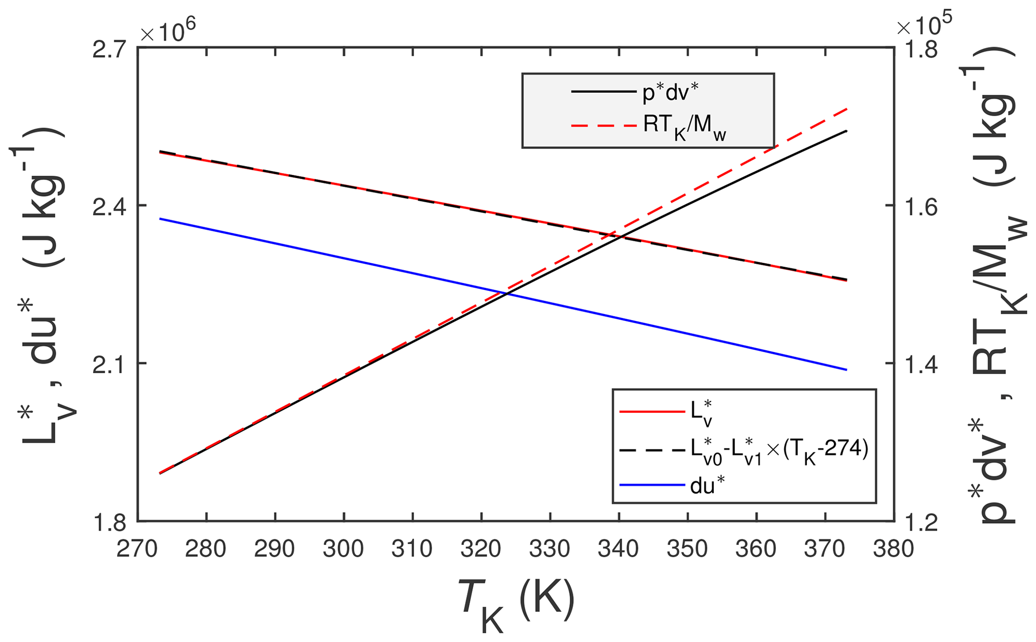
Figure 1The solid red line is the enthalpy of vaporization of pure water, , from Wagner and Pruß (2002), and the dashed black line is a linear approximation to it, where J kg−1 and . The solid blue line is the thermodynamic change in internal energy, du∗, associated with . The other two lines are (solid black) and RTK∕Mw (dashed red). Here TK is the temperature in K, R () is the universal gas constant, and Mw=0.0180153 kg mol−1 is the molecular mass of water vapor.
Paw U et al. (2000, Appendix C), on the other hand, take a different approach to the pΔv term. They do not apply their correction directly to LvE in the SEB equation. Rather they apply their correction to the heat flux, H, based on a change in density of an air parcel associated with mixing newly transpired or evaporated water vapor with the air contained within that air parcel. They pose their correction in terms of an equivalent temperature perturbation, such that after evaporation has occurred the (turbulent + diffusive) transport-driven expansion of the water vapor into the atmosphere surrounding the source of water vapor (e.g., plant stomatal pores and the porous soil) results in a change in the atmospheric density that is associated with a concomitant change in the atmospheric temperature. So in effect Paw U et al. (2000) are using the first law of thermodynamics (expressed in terms of atmospheric processes and the pressure work term) to argue that H should be adjusted to include a small term that is proportional to the mass flux of water vapor, E ().
The present paper employs “classical” thermodynamics to examine (a) the influence that the non-ideality of atmospheric gases can have on the SEB and (b) the methods and conclusions of Paw U et al. (2000, Appendix C) regarding the first law of thermodynamics and the pressure work term's influence on the turbulent heat flux and ultimately the SEB as well. Although it is true that what I develop herein is not necessarily “new” science, some of the theory I employ may well be new to the general environmental and geo-biophysical communities. The present study is divided into two parts. The first examines and quantifies how mixing of air and water vapor as non-ideal (or real) gases, rather than as ideal gases, can impact Lv and the specific heat of moist air. In the second part the first law of thermodynamics is employed to derive the influence water vapor has on potential temperature, which in turn gives rise to an expression, different from that developed by Paw U et al. (2000, Appendix C), relating how the kinematic heat flux is influenced by the mass flux of water vapor, E. In summary, this study shows that any potential corrections to the SEB from either of these two sources are likely to be negligible and certainly much smaller than either Kowalski (2018) or Paw U et al. (2000) propose.
The next three sections are a purely theoretical argument intended to estimate the influence that a mixture of non-ideal gases (water vapor and dry air) can have on the SEB near standard pressure and temperature (STP) by comparing the enthalpy of vaporization of water and the specific heat of moist air associated with ideal gases and non-ideal gases. Here “near STP” will be understood as pressures between about 70 and 105 kPa and temperatures between about 0 and 100 ∘ C or so – or an atmospheric state typical of near-surface conditions on earth.
2.1 Enthalpy of vaporization
The enthalpy of vaporization for pure water into an atmosphere of pure water vapor (see either Wagner and Pruß, 2002, or Harvey and Friend, 2004) is expressed as
where (J kg−1 or J mol−1) is the enthalpy of vaporization for pure liquid water into an atmosphere of pure saturated water vapor, (J kg−1 or J mol−1) is the specific enthalpy of saturated vapor, and (J kg−1 or J mol−1) is the specific enthalpy of pure liquid water. Note (a) that the asterisk superscript (∗) will be used to denote a pure quantity (as opposed to a mixture which will not be superscripted) and (b) that the researchers cited above essentially employ the Clausius–Clapeyron equation to determine . Of course, liquid water under near-earth-surface conditions will not be composed solely of pure liquid water. Rather it will be a mixture of pure liquid water and, e.g., dissolved atmospheric gases (O2, CO2, CH4, etc.) and possibly any number of dissolved organic and inorganic compounds (e.g., mineral salts, organic acids). But for the present study, it is unnecessary to consider this additional complexity. Figure 1 includes plots of as a function of temperature, TK (K), computed using the formulations of Wagner and Pruß (2002) (red line), and a linear approximation to it (black line) over the plotted temperature range.
Also included in Fig. 1 are the two components of the specific enthalpy of vaporization (i.e., the change in internal energy, du∗, and the pressure work term, ), where accordingly . For this figure du∗ is calculated as the difference and is estimated as follows:
where pv (Pa) is the vapor pressure, ρv (kg m−3) is the vapor density and ρl (kg m−3) is the density of liquid water. The numerical algorithms used for pv, ρv and ρl are from Wagner and Pruß (2002). But since ρl≫ρv it follows that . In turn the ideal gas law yields – also shown in Fig. 1 – where R () is the universal gas constant and Mw (kg mol−1) is the molecular mass of water. The three quantities du∗, , and RTK∕Mw are included in Fig. 1 primarily for the sake of completeness and to give some sense of their relative contributions to . Figure 1 indicates that , meaning that is a relatively small component of .
Next, consider a system of Nd mols of dry air and Nl mols of pure liquid water separated from one another by an impermeable membrane. Both are at the same temperature TK,init and the pressure of the dry air is pd (Pa). Further assume that this dry air–liquid water system is isolated, i.e., that it cannot exchange mass or energy or interact mechanically with its surroundings. The total enthalpy of this system is (J). This will now be considered the initial state of the system.
After removing the membrane the final state of the system occurs after Nv mols of liquid has evaporated and diffused throughout the volume of dry air to the point of saturation, where of course Nv≤Nl, to ensure that there is enough liquid to achieve saturation. Note: it is possible to calculate Nv, because Nv=Nv,sat, but for the present purposes this is not necessary. The final state now comprises Nd mols of dry air, Nl−Nv mols of pure liquid water and Nv mols of water vapor. For an ideal gas the final pressure is pv,sat (Pa), but for a non-ideal gas the saturated vapor pressure is fpv,sat (Hyland and Wexler, 1983; Goff, 1949), where is termed the enhancement factor and near STP (Hyland and Wexler, 1983; Nelson and Sauer, 2004). Consequently, the final pressure of the water vapor will exceed pv,sat by a small amount. On the other hand, the final pressure of the dry air, pd,final (Pa), will be slightly less that pd because the final gas volume of the system will be slightly greater than the initial volume due to the decrease in the volume of liquid with the evaporative loss of Nv mols of liquid. In the present scenario this difference between the final and initial pressures is small: ≈0.001pd. Because both f and this relative pressure difference are so small and they tend to compensate for one another, it is reasonable to ignore both effects and approximate the final total pressure, pa (Pa), as simply as , meaning that for present purposes evaporation occurring within an isolated system can be considered an archetypical constant pressure process. Nonetheless, it is also worth emphasizing that, in fact, evaporation in the present isolated system (as well as within the atmospheric surface layer) is neither a constant volume process nor a constant pressure process. Rather it is a combination or hybrid of the two processes.
The total enthalpy of the final state of the system is , where ha (J mol−1) is the specific enthalpy of the resulting moist air. But because of evaporative cooling, the temperature of the final state of the system, TK (), is less than TK,init. This change in temperature of the system, δT (K), is defined as . The Appendix examines this temperature difference in more detail. With this last simplification in mind, the change in total enthalpy of the system, ΔHs (J), is
where (e.g., Hyland and Wexler, 1983) and is the dry air molar fraction (mol mol−1) of the moist air, is the vapor molar fraction (mol mol−1) of the moist air, and IB is the excess enthalpy of mixing (e.g., Wormald et al., 1977; Sattar, 2000) that arises because of the non-ideality of the gases (e.g., Hyland and Wexler, 1983).
After some algebraic manipulation the following simplified expression for ΔHs results:
where and . Because both and are functions of temperature, i.e., and , and δT is small in comparison to either TK,init or TK (Appendix A), it is reasonable to approximate as . Similar results hold for , so that the component of ΔHs can be reasonably assumed to be a function of both temperature and the temperature difference. On the other hand, the component of ΔHs is a function only of the final temperature, TK, and is not influenced by δT. This allows the following identification to be made: , where results from the change in phase associated with evaporation and results from the change in temperature. The principal interest of this study is ΔHs,L. Therefore, dividing ΔHs,L by Nv yields
At this point it is important to note that except for the non-ideality of water vapor and dry air, the enthalpy of vaporization of water would be completely independent of the presence of dry air, i.e., . In other words, if not for the non-ideal behavior of these gases Lv would be the sole property of water and would otherwise not be influenced by the presence or absence of dry air.
In general IB is expressed in terms of the second and third virial coefficients (Hyland and Wexler, 1983; Wagner and Pruß, 2002), which are defined by the virial equation of state (Hyland and Wexler, 1983; Sattar, 2000) as follows:
where the subscript “i” refers to water vapor (i= v), dry air (i= d), or moist air (i= a); Bi (m3 mol−1) is the second virial coefficient, Ci (m6mol−2) is the third virial coefficient, and in general Bi and Ci are both functions of temperature, TK; pi is the gas pressure (Pa) and vi is the molar volume (m3 mol−1) of the gas. For this study it is sufficient to consider only the second virial coefficients. For dry air and water vapor Bi=Bi(TK) is determined by empirical curve fitting of observed data. For this study Bv(TK) is taken from Eq. (6) of Harvey and Lemmon (2004) and Bd(TK) is taken from Eq. (10) of Hyland and Wexler (1983). Because moist air is a mixture of dry air and water vapor the second virial coefficient for moist air takes the form (Sattar, 2000), where Bvd (m3 mol−1) is the cross virial coefficient for moist air. For the present study Bvd(TK) is taken from Eq. (15) of Hyland and Wexler (1983). Once the equation of state has been specified, the general expression for IB can be derived (e.g., Sattar, 2000), yielding
The final step is to specify whether the enthalpic change occurs at constant pressure or at constant volume. Although assuming a constant pressure pathway for modeling evaporation into the atmosphere is likely to be more appropriate than assuming a constant volume pathway, both pathways need to be considered here because any evaporation occurring on the earth's surface is going to lie somewhere between these two (bounding) pathways. This is equivalent to specifying pa and pd at the initial and final states. At a constant pressure pa is held constant, so that , where pd(initial state)=pa and pv(final state)=pv,sat, and (for the sake of completeness it should also be noted that) pv(initial state)=0. In this case pa is arbitrarily assigned a value of 101.325 kPa. To evaluate at a constant volume pd is held constant, so . In this case pd is arbitrarily assigned a value of 101.325 kPa. The only difference between these two cases is that the final molar values of Nv and Na() can be different, so that the term paχd in Eq. (7) can vary slightly depending on whether the evaporation is occurring at a constant pressure or a constant volume.
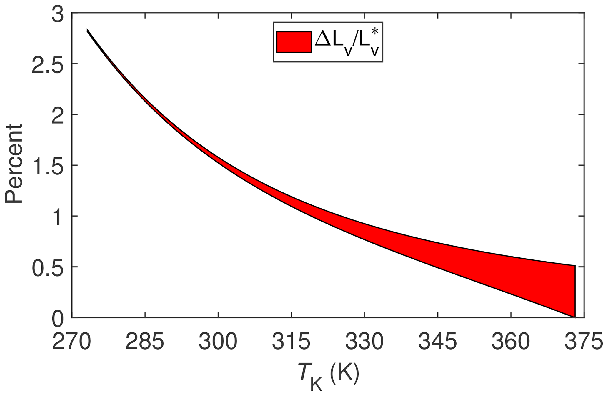
The results of evaluating Eq. (7) for these two different processes are shown in Fig. 2. Note that beginning with this figure and henceforth ΔLv will be used as shorthand for IB∕χv. With the exception of sublimation of ice or snow, these results suggest that surface energy fluxes associated with ET measured at temperatures commonly encountered with micrometeorological techniques (i.e., between about 275 and 325 K) could be underestimated by 1 % to 2.5 % solely on the basis of using an estimate for the enthalpy of vaporization, , that does not allow for the fact that dry air and water vapor are non-ideal gases. Categorically then this underestimate is at least an order of magnitude less that the often observed surface energy imbalance mentioned in the introduction.
2.2 Specific heat
But in many micrometeorological studies of the SEB LvE is only half the story. There is also the sensible or convective heat flux, , where ρa (kg m−3) and ϱa (mol m−3) are the density of the ambient moist air (in mass or molar units) and Cpa () and cpa () are the specific heat of moist air at constant pressure (in units corresponding to the moist air density). is the kinematic heat flux, which is obtained directly from eddy covariance measurements. Assuming ideal gases, is the weighted sum of the specific heats of pure water vapor (subscript v) and pure dry air (subscript d). For the present study , , and are obtained from Eq. (6) of Bücker et al. (2003).
Using Δ to denote the departure from ideality, the derivation of begins with the following (standard thermodynamic) relation (e.g., Curry and Webster, 1999, Eq. 4.29), where cpv and cpl are the specific heats at constant pressure for water vapor (subscript v) and liquid water (subscript l). Combining this relationship, which is valid for both ideal and non-ideal gases, with Eq. (5), it is straightforward to show that
For the present purposes it can be assumed that liquid water always remains pure (or ideal) and, therefore, . Then, identifying Δcpv as and using Eq. (7) above, it follows from Eq. (8) that
To complete the estimate of Δcpa it is necessary to determine χdΔcpd, which is easily deduced from the dry air term (d2Bd∕dT2) in Eq. (9). In this last equation, as well as in Eqs. (5) and (7), the dry air term (any Bd term) is basically meant to account for the effects of dry air interacting with itself. Consequently, it is fairly straightforward to conclude from Eq. (9) that
Combining this last expression for χdΔcpd with that for χvΔcpv yields the final results for as a function of TK, which is shown in Fig. 3 overlaying from Fig. 2.

2.3 Consequences for the surface energy balance
Implications for the SEB of mixing the two non-ideal gases (water vapor and dry air) during evaporation can now be estimated by combining the results for and ΔCp∕Cp. For example, assuming a Bowen ratio of approximately unity (i.e., the magnitudes of H and LvE are approximately the same) and a temperature between say 275 and 325 K, then the term LvE+H in the SEB could be underestimated between 1 % and 1.5 % with micrometeorological techniques due to the non-ideality of water vapor and dry air. Allowing for different values of the Bowen ratio would imply a somewhat broader range of percentage underestimates. But even so, it is unlikely that non-ideality could cause LvE+H to be underestimated by more than 2 %, which, at best, is an order of magnitude less than required to account for the imbalance of the SEB.
This section examines the issue Paw U et al. (2000) address, viz., the “energy associated with evaporation into the atmosphere, necessary for the expansion of eddy parcels against an approximately constant pressure”. In essence the authors are proposing a correction to eddy covariance measurements of turbulent temperature fluctuations (T′) that account for the density change of an air parcel associated with the mixing of a relatively dense fluid (ambient air), with a relatively less dense fluid (water vapor). The following is a slight reformulation of their approach.
For an adiabatic process the first law of thermodynamics can be expressed as
where cv () is the molar specific heat of moist air at constant volume and va (m3 mol−1) is the specific volume of air, which by definition is the reciprocal of the molar air density, ϱa (mol m−3). Switching from differential notation to perturbation notation, Eq. (11) can be written as . By definition, , so it also follows that , which combined with the ideal gas law pAva=RTK yields the following equivalent expression for Eq. (11):
where is defined by Paw U et al. (2000) as “the temperature perturbation equivalent to the energy needed for expansion”. Next they assume that the change in molar air density, , is due to the mol per mol displacement of moist air by water vapor, so that for present purposes , from which is follows that
where the second expression on the right is expressed in mass units (kg) rather than mols; i.e., μ=1.609 is the ratio of the molecular mass of dry air to the molecular mass of water vapor, ρv (kg m−3) is the mass density of water vapor, and ρa (kg m−3) is the mass density of the ambient atmosphere. Equation (13) is a rephrasing of the principal result – Eq. (C3) – of Appendix C of Paw U et al. (2000).
Before proceeding with an alternative approach to deriving an expression for , it is insightful to examine an apparent sign error made by Paw U et al. (2000) in their mathematical development of and its equivalent heat flux – their Eq. (C4). First, they pose their Eq. (C2) as the antecedent to their expression for by asserting that when displacing heavier dry air molecules by lighter water vapor molecules, meaning that the specific volume perturbation should decrease; i.e., . But this contradicts the fact that the specific volume should increase when the density of the (formerly dry) air parcel decreases when displacing heavier molecules by lighter ones. From the discussion in the paragraph immediately preceding the present one – implies combined with the displacement assumption – it follows that , in agreement with expectations. Interestingly, despite this sign error in Eq. (C2), Paw U et al. (2000) have the same sign for their – their Eq. (C3) – as Eq. (13) above; i.e., both expressions yield . Nonetheless, and even more puzzling, is that Paw U et al. (2000) reverse the sign again when they proceed to their Eq. (C4), the succedent to their Eq. (C3). In this step of their development of the heat flux He, generally defined such that , they suggest that . The reason for reversing the sign a second time is not discussed, nor is how this might relate to the pressure work term. But if their goal is to determine an equivalent heat flux associated with a change in density of an air parcel due to the partial displacement of a heavier gas in that air parcel by a lighter gas, then it is reasonable to expect that He>0 because that air parcel would be positively buoyant relative to the surrounding (drier and heavier) air. Assuming this conjecture is true, then this contradiction in the sign of He suggests seeking an alternative approach to determine He. The remaining portion of this study outlines such an alternative.
The final portion of this study attempts to clarify the nature of He and the role of the work term and whether the surface sensible heat flux includes a water vapor term similar to that suggested by Paw U et al. (2000) and recast as Eq. (13) above. I begin with the time-dependent version of the first law of thermodynamics expressed as the conservation law for potential temperature, θ (K), for atmospheric processes:
where dq∕dt represents the heat flow associated with diabatic atmospheric processes, u (m s−1) is the atmospheric velocity, and ∇ is the vector gradient operator. Here the term associated with compressible effects, θ∇⋅u, is included for completeness, although it is not important for the present purposes. Equation (14) is standard and in and of itself is not novel. Nonetheless it does imply an important take-away, which is that the turbulent surface sensible heat flux is more correctly expressed in terms of potential temperature, , rather than in terms of temperature, . This is principally because explicitly includes the effects of any change in ambient pressure and the concomitant work done on or to the atmosphere during turbulent atmospheric processes. Note: for the sake of completeness w (m s−1) is the vertical velocity and the ′ notation is standard and refers to Reynolds averaging. Having identified potential temperature as the key variable for discussion, the next step is to examine the influence moisture has on θ.
Including the effects of water vapor on potential temperature yields the following relation (e.g., Curry and Webster, 1999, Eq. 2.66):
where p00=100 kPa is a constant reference pressure; , for which Cpd is the specific heat for dry air and consequently is an extremely good approximation; and (kg kg−1) is the specific humidity of moist air. Equation (15) clearly indicates that θ is dependent on moisture. Although this dependency is extremely weak, the purpose here is to assess the influence of on the θ′ using Eq. (15) and to compare the result with Eq. (13). A sketch of the derivation follows.
Linearize Eq. (15) first by noting that near-surface atmospheric conditions (i.e., qv<0.04 and or 0.26qv<0.011 and ) are sufficient to guarantee that and second by assuming that the perturbation quantities are small compared to their background levels (which will be denoted by an overbar). This yields
where , , and for later use . Substituting α′ into Eq. (16) yields
where . Next is the evaluation of by expanding and linearizing in terms of and . This yields . The ideal gas law for ambient air yields and, therefore, . Substituting this last expression for into Eq. (17) yields
or
where . At this point it is important to reiterate that for near-surface conditions .
Equation (19) suggests that water vapor contributes two different “corrections” to the kinematic heat flux. First, the middle term on the right-hand side of this equation is due to the overall presence of water vapor, , and second, the last term on the right-hand side of Eq. (19) and the term of interest in this study, results from fluctuations in water vapor, . Although Eqs. (13) and (19) have somewhat different definitions of heat flux, it is still possible to assess the appropriateness of the displacement assumption made by Paw U et al. (2000) by numerically comparing the dimensionless coefficient μR∕cv in Eq. (13) with γ in Eq. (19). Noting that , then . In other words, and, therefore, the approach followed by Paw U et al. (2000) predicts significantly more turbulent heat flux associated with the water vapor flux than does the approach based on potential temperature (initiated above with Eq. 14). Even allowing for the difference between potential temperature and TK does not really change this result by more than 10 % because for conditions being considered here.
This difference between Paw U et al. (2000) and the present result is made more explicit by comparing the next two expressions. The first expression derives from combining Eq. (13) for with the equivalent heat flux, , from Paw U et al. (2000). This yields the following generalization of the Paw U et al. (2000) result:
where Rd=287 . The second expression results by identifying the equivalent potential temperature, , associated with the water vapor perturbation, , in Eq. (19), i.e., , and combining it with the expression for the equivalent heat flux, He, appropriate to Eq. (14), i.e., . This yields
It is not possible to reconcile these two expressions, which brings into question the validity of the displacement assumption of Paw U et al. (2000) (i.e., ), on which Eq. (20) is based. But to truly assess the cogency of this assumption and any enthalpic changes associated with mixing of the dry air and water vapor requires a better description of the physical processes and the initial and final states involved than Paw U et al. (2000) provide. Nevertheless, since they are addressing evapotranspiration, it seems reasonable to assume they are envisioning the final state of the evaporative process. In this case the work done to/by the atmosphere associated with the expansion of water vapor into the atmosphere is appropriately included in the enthalpy of vaporization as previously discussed and, consequently, the displacement assumption would result in over-counting the work term. On the other hand, if they are describing the enthalpic changes associated with rising plumes of warm moist air associated with density differences between very moist air near the surface and drier and therefore, denser air above the near surface, then the methods and results outlined by Eqs. (14), (15), and (21) above are more appropriate.
The present study has explored some of the issues involving the surface energy balance (SEB) and the thermodynamics of evaporation of water into the atmosphere. Specifically I have looked at (a) the influence that molecular interactions between water vapor and dry air (non-ideality of atmospheric gases) could have on estimates of Lv and Cp and the SEB and (b) the impact that fluctuations of atmospheric water vapor could have on the surface heat flux. At typical atmospheric temperatures (275–325 K), the influence of the first effect is probably on the order of about 1 %–2 % and the second is about 0.4 %. Consequently, these phenomena acting either independently or in consort are too small to be of any real significance in explaining the lack of closure of the SEB. This result should not be surprising, but because these issues may not be well known to the micrometeorological and geo-biophysical communities, it seemed worthwhile to attempt to verify this supposition quantitatively.
This Appendix derives the relationship between δT and Nv, Nd and Nl appropriate to evaporative cooling of the isolated thermodynamic system discussed in Sect. 2.1 of the main text. Achieving this requires an approach similar to that used when calculating the wet bulb temperature (e.g., Curry and Webster, 1999). The formal expression for the first law of thermodynamics for the system under consideration is
where the subscripts f and i refer to the final and initial states; Qf−Qi (J) is the total heat exchanged by the system and its environment, which must be 0 since the system is isolated from its environment; Cps (J K−1) is the bulk heat capacity of the composite system (vapor + dry air + pure liquid water) at constant pressure so that the change in the heat content of the system, (CpsTK)f−(CpsTK)i, must exactly cancel the change in the enthalpy of the system , which is expressed here in terms of the water vapor component. assumes that water vapor is an ideal gas (an assumption that is sufficient for the present purposes) and Mv (kg mol−1) the molecular mass of water vapor. Simplifying this expression begins by identifying
and
where N refers to the number of mols of any particular component (subscript d for dry air, v for vapor, and l for liquid); M refers to the molecular mass of that component; cp () refers to the specific heat at constant pressure of that component; and Ml=Mv has been used for the right-hand side of the last expression.
Combining these last two expressions with Nvi=0 and after dividing the resulting expression by Mv yields
where the δT term on the left-hand side and the term on the right-hand side are evaluated at TK (the final temperature), and the first term on the right-hand side, , is evaluated at the initial temperature TKi. The order of magnitude calculation is facilitated by dividing the last expression by cplTKi, by noting that and that and by ignoring the relatively weak temperature dependency of the various cps. This yields
The last step to deriving assumes that J kg−1 and requires noting that for the temperature range , and J kg−1. These last conditions yield the final result:
For the isolated thermodynamic system discussed in the present study it is also valid to assume that Nv≪Nd, which in turn is sufficient to guarantee that δT≪TKi, meaning that the temperature change associated with evaporative cooling should be quite small.
The computer code used in this study was developed using MatLab version 2017b and is publicly available along with any output data at the Forest Service Research Data Archive: https://doi.org/10.2737/RDS-2019-0042 (Massman, 2020).
The author declares that there is no conflict of interest.
The author would like to thank Allan Harvey for his insights and his significant time and efforts involving Sect. 2 of this work. I also gratefully acknowledge Kyaw Tha Paw U, Grant Petty, Jim Wilczak, and Ned Patton for their comments during the development of this work.
This paper was edited by Stan Schymanski and reviewed by Andrew Kowalski, Grant Petty, and one anonymous referee.
Bücker, D., Span, R., and Wagner, W.: Thermodynamic property models for moist air and combustion gases, J. Eng. Gas Turb. Power, 125, 374–384, 2003. a
Curry, J. A. and Webster, P. J.: Thermodynamics of Atmospheres and Oceans, Academic Press, San Diego, CA, USA, 471 pp., 1999. a, b, c
Geiger, R., Aron, R. H., and Todhunter, P.: The climate near the ground, Sixth Edition, Rowan and Littlefield Pub. Inc., Lanham, MD, USA, 584 pp., 2003. a
Goff, J. A.: Standardization of thermodynamic properties of moist air, Heat.-Piping-Air Cond., 21, 118–128, 1949. a
Harvey, A. H. and Friend, D. G.: Physical properties of water, in: Aqueous Systems at Elevated Temperatures and Pressures, edited by: Palmer, D. A., Fernández-Prini, R., Harvey, A. H., Elsevier, Amsterdam, the Netherlands, 1–27, 2004. a
Harvey, A. H. and Lemmon, E. W.: Correlation for the second virial coefficient of water, J. Phys. Chem. Ref. Data, 33, 369–376, 2004. a
Hyland, R. W. and Wexler, A.: Formulations for the thermodynamic properties of dry air from 173.15 K to 473.15 K and saturated moist air from 173.15 K to 372.15 K, at pressures to 5 MPa, ASHRAE Tran., 89, 520–535, 1983. a, b, c, d, e, f, g, h
Kowalski, A. S.: Technical note: rectifying systematic underestimation of the specific energy required to evaporate water into the atmosphere, Hydrol. Earth Syst. Sci. Discuss., https://doi.org/10.5194/hess-2018-195, 2018. a, b, c
Leuning, R., van Gorsel, E., Massman, W. J., and Issac, P. R.: Reflections on the surface energy imbalance problem, Agr. Forest Meteorol., 156, 65–74, 2012. a
Massman, W. J.: Data and source code for “Impacts of non-ideality and the thermodynamic pressure work term pΔv on the Surface Energy Balance”, Forest Service Research Data Archive, Fort Collins, CO, USA, https://doi.org/10.2737/RDS-2019-0042 2020. a
Nelson, H. F. and Sauer Jr., H. R.: Thermodynamic properties of moist air: −40 to 400 degrees Celsius, J. Thermophys. Heat Tr., 18, 135–142, 2004. a
Oncley, S. P., Foken, T., Vogt, R., Kohsiek, W., DeBruin, H. A. R., Bernhofer, C., Christen, A., van Gorsel, E. Grantz, D., Feigenwinter, C., Lehner, I., Liebethal, C., Liu, H., Mauder, M., Pitacco, A., Ribeiro, L., and Weidinger, T.: The energy balance experiment EBEX-2000, Part I: Overview and energy balance, Bound.-Lay. Meteorol., 123, 1–28, 2007. a
Paw U, K. T., Baldocchi, D. D., Meyers, T. P., and Wilson, K. B.: Correction of eddy-covariance measurements incorporating both advective effects and density fluxes, Bound.-Lay. Meteorol., 97, 487–511, 2000. a, b, c, d, e, f, g, h, i, j, k, l, m, n, o, p, q, r, s, t
Sattar, S.: Thermodynamics of mixing real gases, J. Chem. Educ., 77, 1361–1365, 2000. a, b, c, d
Twine, T. E., Kustas, W. P., Norman, J. M., Cook, D. R., Houser, P. R., Meyers, T. P., Prueger, J. H., Starks, P. J., and Wesely, M. L.: Correcting eddy-covariance flux underestimates over a grassland, Agr. Forest Meteorol., 103, 279–300, 2000. a
Wagner, W. and Pruß, A.: The IAPWS formulation 1995 for the thermodynamic properties of ordinary water substance for general and scientific use, J. Phys. Chem. Ref. Data, 31, 387–535, 2002. a, b, c, d, e
Wormald, C. J., Lewis, K. L., and Mosedale, S.: The enthalpies of hydrogen + methane, hydrogen + nitrogen, methane + nitrogen, methane + argon, and nitrogen + argon at 298 and 201 K at pressures up to 10.2 MPa, J. Chem. Thermophys., 9, 27–42, 1977. a