The impact of initial conditions on convection-permitting simulations of a flood event over complex mountainous terrain

Western Norway suffered major flooding after 4 d of intense rainfall during the last week of October 2014. While events like this are expected to become more frequent and severe under a warming climate, convection-permitting scale models are showing their skill with respect to capturing their dynamics. Nevertheless, several sources of uncertainty need to be taken into account, including the impact of initial conditions on the precipitation pattern and discharge, especially over complex, mountainous terrain. In this paper, the Weather Research and Forecasting Model Hydrological modelling system (WRF-Hydro) is applied at a convection-permitting scale, and its performance is assessed in western Norway for the aforementioned flood event. The model is calibrated and evaluated using observations and benchmarks obtained from the Hydrologiska Byråns Vattenbalansavdelning (HBV) model. The calibrated WRF-Hydro model performs better than the simpler conceptual HBV model, especially in areas with complex terrain and poor observational coverage. The sensitivity of the precipitation pattern and discharge to poorly constrained elements such as spin-up time and snow conditions is then examined. The results show the following: (1) the convection-permitting WRF-Hydro simulation generally captures the precipitation pattern/amount, the peak flow volume and the timing of the flood event; (2) precipitation is not overly sensitive to spin-up time, whereas discharge is slightly more sensitive due to the influence of soil moisture, especially during the pre-peak phase; and (3) the idealized snow depth experiments show that a maximum of 0.5 m of snow is converted to runoff irrespective of the initial snow depth and that this snowmelt contributes to discharge mostly during the rainy and the peak flow periods. Although further targeted experiments are needed, this study suggests that snow cover intensifies the extreme discharge instead of acting as a sponge, which implies that future rain-on-snow events may contribute to a higher flood risk.

1 Introduction

Heavy rainfall, with local amounts exceeding 350 mm, fell over the coastal and mountainous areas of western Norway between 26 and 29 October 2014. The event caused widespread flooding, with 16 stations registering discharge above the 50-year flood threshold (Langsholt et al., 2015). The severe flooding of many regional river systems destroyed infrastructure, houses and isolated towns. Overall, the damage exceeded NOK 131.6 million, or roughly USD 16.4 million (Dannevig et al., 2016). A list of reports were produced (in Norwegian), e.g. “October flood in western Norway 2014” (Dannevig et al., 2016) and “The flood in western Norway October 2014” (Lansholt et al., 2015), from the Norwegian Water Resources and Energy Directorate (NVE) that documented the rainfall and discharge records as well as the societal impacts. For flood hazards such as this, it is a challenge to forecast/hindcast the hydrological response due to the complex terrain and the events' complex spatial and temporal characteristics. However, with extreme precipitation over this region projected to increase significantly over the coming decades (e.g. Hanssen-Bauer et al., 2017), the need to reliably reproduce such events is high for both climate researchers and operational professionals.

1.1 Norwegian flood types, changes and rain-on-snow

The complex and varying terrain of Norway divides the country into different climatic zones, and flood-generating processes vary by region. For example, northern and eastern Norway are mainly prone to spring snowmelt floods, whereas southern and western Norway are dominated by rain-induced floods (Vormoor et al., 2015). According to recent studies, snowmelt-generated floods have decreased and have occurred earlier in the spring in recent decades (Vormoor et al., 2016; Pall et al., 2019). At the same time, rain-dominated floods are increasing in frequency (Vormoor et al., 2016). This is consistent with observed increases in precipitation (Dyrrdal et al., 2012) and streamflow (Stahl et al., 2010; Wilson et al., 2010), and these trends are projected to continue into the future (Hanssen-Bauer et al., 2017; Sorteberg et al., 2018). Although temperatures are increasing, much of the winter precipitation in inland catchments will continue to fall as snow until at least the middle of the century (Hanssen-Bauer et al., 2017). However, as the temperature rises, many of these catchments may experience more rain-on-snow events. Warm and often windy conditions during such events can cause substantial additional snowmelt, which can exacerbate an already dangerous flooding event (Marks et al., 1998, 2001). In fact, for many catchments in the world, such as in the western US, rain-on-snow events are important for the prediction of flood responses and risk (Berghuijs et al., 2016; Musselman et al., 2018). While earlier snowmelt is decreasing the frequency of such events in the late spring and at low altitudes, both the magnitude and frequency of rain-on-snow events are increasing during winter in central Europe (Freudiger et al., 2014) and likely also in Norway. Pall et al. (2019) used a high-resolution (1 km) seNorge data set to construct the climatology of rain-on-snow occurrence in mainland Norway for recent decades. They found an increase in rain-on-snow events in high-elevation areas across the mainland in winter–spring. Given the dependence of floods in Norway on a complex interplay between factors such as variations in elevation, temperature gradients (e.g. between land and ocean), orographic interactions, existing snow and soil moisture distributions, it is critical to run models (either dynamical or statistical) at resolutions that can capture this complexity. However, this requirement presents challenges of its own. Despite this, the rain versus snowmelt contribution to the flow can be important in determining the flood-generation processes for Norway and can be particularly sensitive to the vertical temperature gradient.

1.2 Forcing data and convection-permitting modelling

In order to improve our scientific understanding as well as predictions and projections of flooding, high-quality meteorological forcing data are crucial. A lack of detailed precipitation records that accurately represent spatial and temporal variability at both the basin and regional scales presents well-known challenges to hydrological modelling. In mountainous areas, like western Norway, where precipitation is strongly influenced by the terrain, spatial patterns of precipitation are not well captured by either sparse gauge data or gridded precipitation data sets (e.g. satellite-based products or high-resolution interpolation-based data sets). High-resolution, convection-permitting modelling has exhibited great promise in addressing these issues and has the potential to be a powerful tool for hydrological prediction (Prein et al., 2015, 2016, 2017; Smiatek et al., 2016; Kendon et al., 2017; El-Samra et al., 2018; Poschlod et al., 2018; Avolio et al., 2019). Pontoppidan et al. (2017) investigated the importance of kilometre-scale resolution on the aforementioned flooding event in October 2014 over western Norway and found that convection-permitting simulations (∼3 km grid spacing) from the Weather Research and Forecasting (WRF) model substantially improved the representation of precipitation compared with a coarser 9 km grid spacing simulation. This improvement was seen both in terms of absolute values and spatial–temporal distribution. The largest improvement was seen in a simulation with a resolution jump from parameterized to explicitly resolved convection (e.g. from 9 to 3 km over western Norway). Several previous studies over other regions have also demonstrated the added value of convection-permitting modelling for extreme weather impact studies in regions with complex terrain. For example, Maussion et al. (2011) showed an improved representation of precipitation in a convection-permitting (2 km) simulation when compared with satellite products over the Himalayan region. El-Samra et al. (2018) suggested that downscaling over complex terrain requires a horizontal grid resolution of 3 km or higher in order to improve the forecasting of mean and extreme temperatures and capture the orographic precipitation climatology. Conversely, coarse-resolution (∼9 km) simulations miss the impact of orography on temperature and precipitation. Additionally, the studies of Rasmussen et al. (2011, 2014) found that a spatial and temporal depiction of snowfall that is adequate for water resource management over the Colorado River headwaters region can only be achieved with the appropriate choice of model grid spacing and parameterizations. The modelling systems that are capable of accurately depicting the atmosphere at these scales now increasingly incorporate other regional system components such as crops, urban features and, of most relevance to the present study, hydrology.

1.3 A dynamical hydrometeorological model: WRF-Hydro modelling system

The Weather Research and Forecasting Model Hydrological modelling system (WRF-Hydro) is a model coupling framework designed to link multi-scale process models of the atmosphere and terrestrial hydrology (Gochis et al., 2018). It runs both in fully coupled (two-way) or uncoupled (one-way, from atmosphere to land) modes and is intended to serve as both a hydrometeorological prediction system and a research tool. The system has been applied in studies around the world (e.g. Senatore et al., 2015; Givati et al., 2016; Arnault et al., 2016; Xiang et al., 2017; Naabil et al., 2017; Verri et al., 2017; Lin et al., 2018; Rummler et al., 2019). It is currently in use operationally as a key component of the United States National Water Model where it expands the number streamflow forecast points from ∼3600 points to ∼2.7 million river reaches (https://water.noaa.gov/about/nwm, last access: 4 February 2020). WRF-Hydro has also been applied in Africa (Arnault et al., 2016; Kerandi et al., 2018), in the Himalayas (Li et al., 2017), in Italy (Verri et al., 2017; Senatore et al., 2015) and in the eastern Alps (Rummler et al., 2019) with promising results, and it shows potential for use in runoff forecasting, water resource planning and climate change impact assessments. However, despite its application across a diverse array of catchments and research questions, the system has yet to be evaluated for a case in Norway.

There are still challenges with respect to discharge prediction by WRF-Hydro, and the model's performance varies across geographic regions and climate. For example, it simulated flood events in the Black Sea region fairly well if both model calibration and WRF data assimilation were performed jointly, whereas the streamflow obtained with raw WRF precipitation was generally very poor (Yucel et al., 2015). It also simulated a full annual cycle of the Crati River basin in southern Italy with a Nash–Sutcliffe efficiency (NSE) of 0.8 using observed precipitation, whereas it only achieved a NSE of 0.27 using simulated precipitation (a perfect model result is a NSE of 1.0, and a NSE of 0 indicates that the model predictions are as accurate as the mean of the observed data) (Senatore et al., 2015). Naabil et al. (2017) applied WRF-Hydro in a test case over west Africa for water resource management and found that further improvements via proper model calibration as well as consideration of the impacts of model biases at the dam level were needed, although the model captured the attributes of the streamflow. Furthermore, Verri et al. (2017) demonstrated that the performance of WRF-Hydro was severely affected by various components including simulated precipitation, initial conditions and the calibration/validation of discharge hydrography. In Texas, WRF-Hydro has shown promise as a forecast tool; however, it suffers from poor prediction skill in areas with anthropogenically altered flows, where both the surface runoff and the base flow are underpredicted (Lin et al., 2018). Additional studies also noted the sensitivity of WRF-Hydro to the initial conditions (the spin-up time) (Román-Cascón et al., 2016; Bonekamp et al., 2018; Verri et al., 2017). In order to obtain a stable WRF-Hydro simulation, a spin-up period is required, which depends on the quality of the model input and soil data. Therefore, the impact of the spin-up time needs to be assessed on per-case basis, as it likely depends on local conditions.

1.4 Objectives of the paper

Due to the traditional separation of hydrological and atmospheric modelling communities, significant gaps exist in our knowledge of the full-chain responses to hydrometeorological extremes, from the circulation/transport of moisture to precipitation to discharge. WRF-Hydro is designed to link these components and their characteristic scales to provide a modelling framework that can address these gaps (Gochis et al., 2018). It enables improved simulation of land surface hydrology as well as energy states and fluxes at a high spatial resolution (typically 1 km or less). It can be used in either “offline” (uncoupled to the atmospheric component of the model) or “fully coupled” modes (the hydrological model components have two-way interactions with the atmospheric component) (Gochis et al., 2015).

In this study, we employ WRF-Hydro in western Norway to investigate the meteorological and hydrological processes driving the October 2014 flooding. To our knowledge, this is the first study using a complete meteorological–hydrological modelling approach to characterize a precipitation-induced extreme flooding event in Norway. The causal mechanisms and evolution of this particular flood event are examined. In addition, we explore the sensitivity of the discharge to different initial conditions such as soil and snow.

The work is based upon the study of Pontoppidan et al. (2017) for the simulation of the meteorological processes and the hydrological impact. As such, an “offline” (“uncoupled”) configuration for the WRF-Hydro model is chosen. This is due to the fact that we primarily aim to understand the flood event in the context of its hydrological response to the weather forcing and land surface conditions. Feedbacks between the atmosphere and land, although important, generate second-order effects that likely only have a small impact within such a short duration event. Moreover, the offline mode of the WRF-Hydro system is preferable for our study, as it provides a clearer interpretation of the results, identification of uncertainties in the water budget, and assessment of the sensitivity to critical parameters in the atmospheric and hydrological components (Li et al., 2017).

The remainder of the paper is structured as follows: in Sect. 2, a description of the study area and data is presented; the methods, including a description of the WRF-Hydro set-up and experiment design, the model calibration and the benchmark evaluation, are outlined in Sect. 3. In Sect. 4, the results concentrate on the model calibration, the benchmark evaluation and the precipitation evaluation, and the impacts of initialization (spin-up time) and prescribed snow cover are examined. Finally, the main discussion and conclusions are presented in Sects. 5 and 6 respectively.

2 Study area and data

2.1 Study area

Our four study catchments are located in western Norway, where the landscape is dominated by steep orography and complex terrain, due to the fjords, and elevation varies from sea level to more than 2400 m (Fig. 1). The complex terrain both enhances the precipitation and generates large local differences in the precipitation distribution (e.g. Reuder et al., 2007; Pontoppidan et al., 2017). Norway is positioned at the exit of the North Atlantic storm track, which brings low-pressure systems and associated frontal precipitation towards the west coast on a regular basis during autumn and winter. Western Norway is the wettest part of the country (Hanssen-Bauer and Førland, 2000) and annual precipitation exceeds 3000 mm in several places. However, the precipitation in the region shows high spatial variability; for example, Kvamskogen–Jonshøgdi (60.389^∘ N, 5.964^∘ E) records 3151 mm, whereas Vossevangen (60.625^∘ N, 6.426^∘ E), which is only 36.6 km away, only receives 1280 mm (Førland, 1993; see Fig. 1 in this paper for site locations).

Figure 1 The locations of the study catchments in western Norway. (a) The outer domain (resolution 9 km) and the location of the inner domain (d02; shown using a white frame). (b) A zoomed in view of the inner domain (resolution 3 km) showing the topography and the four study catchments' boundaries as well as details about the ground-based observation stations, including discharge stations, HOBO rain gauges and MET weather stations (from https://www.met.no/, last access: 4 February 2020), for model calibration and further performance evaluation.

2.2 Hydrometeorological conditions

October 2014 was wetter than usual in western Norway. The situation was maintained by an atmospheric river and the passage of multiple frontal systems with moderate to heavy precipitation. On 26 October, 2 d before the flooding event, a low-pressure system with associated fronts passed over western Norway and delivered considerable amounts of precipitation. A cold front passed through the area at midnight on the 27 October, advecting colder and drier air into the area for a short period. Simultaneously, a disturbance over Scotland developed and moved towards Norway, leaving western Norway in the warm sector of an intensifying low-pressure system. Once again large amounts of precipitation fell from midday on the 27 October to early evening on the 28 October. The associated cold front passed over the Bergen area in the afternoon, and the precipitation intensity decreased with its passage. Due to the already saturated soil and several days with more or less continuous rainfall, the flood peaked in the Voss area in early evening of the 28 October (Pontoppidan et al., 2017).

According to the NVE report by Langsholt et al. (2015), there was shallow snow cover in high-altitude areas east of the catchments. In Voss, however, where our four catchments are located, there was no snow in the snow depth water equivalent maps released by the NVE. These maps are made from model simulations based on the NVE snow observations. Discharge in each of the study catchments was over the 50-year return level. On the 29 October 2014, the daily discharge record held since 1892 was broken at the Bulken station, located at the outlet of Vangsvatnet (Langsholt et al., 2015).

2.3 Observational data

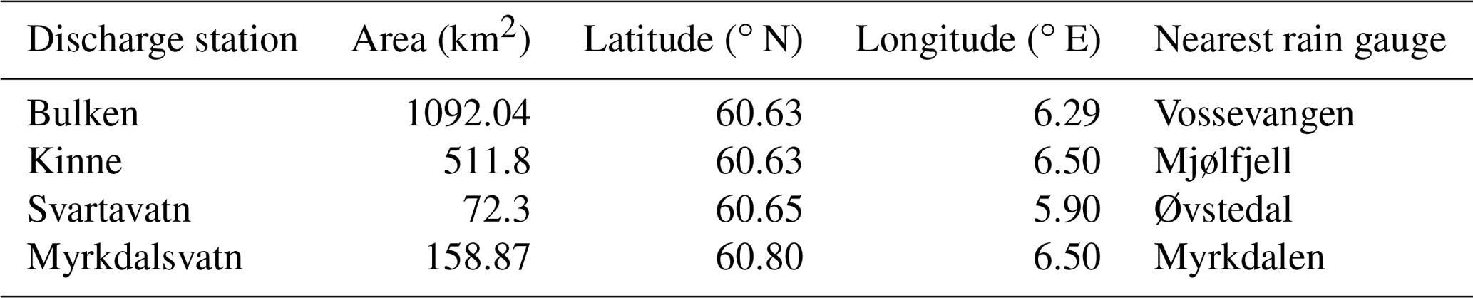
We use 43 precipitation gauges from the Norwegian Meteorological Institute (MET Norway) situated in and around the catchments, with either hourly or daily precipitation data. Typically, rain gauges in Norway are deployed at low elevations and in valleys, resulting in skewed precipitation distributions. To rectify this, 11 HOBO rain gauges, which provide hourly data, were deployed at higher elevations in a transect from the coast to inland regions (Pontoppidan et al., 2017). A table with station details can be found in Pontoppidan et al. (2017). Four discharge stations from the NVE are used for WRF-Hydro model discharge calibration and validation (see Table 1). It should be noted that the drainage basin of the Bulken catchment includes the Kinne and Myrkdalsvatn catchments. In addition, four precipitation gauges from MET Norway, which are the nearest stations in the four basins, are chosen for precipitation evaluation in Sect. 4.3 (Table 1). Figure 1 shows the locations of the four catchments and the rainfall and discharge gauge measurement sites.

Table 1 The list of observed discharge stations and weather stations located in each of the catchments.

3 Methods

3.1 WRF domain design

The Advanced Research WRF (WRF-ARW) model version 3.9.1 is set up with two nested domains with a spatial resolution of 9 and 3 km respectively (Fig. 1). The lateral boundaries are forced with the 6-hourly ERA-Interim reanalysis with a spatial resolution of 0.75^∘ (Dee et al., 2011). The sea surface temperatures (SST) are also updated every 6 h. The model is run with 40 vertical levels in all domains.

The choice of the microphysical scheme is important for precipitation. Previous studies of mountain precipitation using WRF have shown that the Thompson microphysical scheme (Thompson et al., 2008) performs well (Collier et al., 2013; Maussion et al., 2014; Rasmussen et al., 2011, 2014; Li et al., 2017); this is particularly true in areas with mixed hydrometeors, as it computes cloud water, rain water, snow, graupel and ice. The scheme was also successfully used in a previous study on this specific event (Pontoppidan et al., 2018). The grid spacing in the outer domain is in the so-called “grey zone” (5–10 km) where convection may or may not be explicitly resolved; therefore, we tested the impact of the convection parameterization on precipitation. The results showed negligible differences between simulations with the convection scheme on and off. Here, we present the results from the simulations with the convection parameterization turned off. The Yonsei University scheme (Hong et al., 2006) is used for the planetary boundary layer, the RRTM scheme is used for long-wave radiation (Mlawer et al., 1997) and the RRTMG scheme is used for short-wave radiation (Iacono et al., 2008). The Noah land surface model (“Noah LSM”, Mitchell et al., 2005) is used as the surface scheme, which has a bulk layer simple canopy and snow model. In the Noah LSM, the snow cover area fraction within a model grid is determined as a function of snow water equivalent (SWE) using a generalized snow depletion curve. When snow is on the ground, the model considers a bulk snow–soil–canopy layer and computes surface temperature at each time step. The snow surface temperature for the snowpack is estimated in two steps. Firstly, the energy balance between the snowpack, topsoil layer and the overlying air is calculated to obtain an intermediate temperature. This temperature can rise above freezing even when the model grid is fully covered with snow. Secondly, the effective temperature is adjusted by accounting for the fractional snow cover on the ground (Livneh et al., 2010).

Additional configuration details include a model time step of 18 s over the inner domain and the use of spectral nudging to keep the large-scale flow consistent with the driving ERA-Interim reanalysis. This approach proved to be useful when reproducing extreme precipitation events due to the better resolution of synoptic-scale features over the North Atlantic (Heikkilä et al., 2011). Spectral nudging (Radu et al., 2008) is only applied in the outer domain leaving the model free to create its own structures in the inner domain. In the present case, nudging is only applied above the boundary layer and only on wavelengths longer than 585 km.

3.2 WRF-Hydro modelling system

Version 3.0 of the WRF-Hydro modelling system is used in this study. A comprehensive description of the model system can be found in Gochis et al. (2015). In our study, the saturated subsurface overflow routing, surface overland flow routing, channel routing and base-flow modules are activated. The overland flow routing adopts a 2-D diffusive wave formulation (Julien et al., 1995), and the channel routing is calculated by a 1-D variable time-stepping diffusive wave formulation. In addition, a bucket model for base flow is used that is associated with a groundwater reservoir with a conceptual depth and a related conceptual volume. A few lakes in the Bulken catchment are not considered in this study due to a lack of data.

WRF-Hydro is set up to run offline using the WRF atmospheric simulations as input (see Sect. 1). The sub-grid routing processes are executed at a 300 m grid spacing, and the surface physiographic files are prepared by ArcGIS 10.6 (Sampson and Gochis, 2018). The physiographic file includes high-resolution terrain grids specifying the topography, a channel grid, flow direction, stream order (for channel routing), a groundwater basin mask and the position of stream gauging stations, which are the outlets for water routing out across the landscape (Gochis et al., 2015). There are four stream orders in the network of the study catchments shown in Fig. 2.

Figure 2 Map of the physiographic grid for routing processes showing the four study catchments (Svartavatn, Bulken, Myrkdalsvatn and Kinne), the discharge stations and the stream orders in the inner domain used for hydrological modelling in the WRF-Hydro model system. It is worth noting that the Bulken catchment is downstream of the Kinne and Myrkdalsvatn catchments, which means that the drainage basin of the Bulken catchment comprises both the Kinne (pink) and Myrkdalsvatn (light green) catchments in the study.

3.3 Model calibration

Two-step calibration of WRF-Hydro is performed in the study. First, we select the most sensitive parameters from a wide range of parameters. These include the saturation soil conductivity (in SOILPARM.TBL), the optimum transpiration air temperature (in VEGPARM.TBL), the infiltration parameter (in the surface runoff parameterization of GENPARM.TBL), the Manning roughness coefficients (in the channel routing of CHANPARM.TBL), the groundwater bucket model exponent (in the groundwater bucket model of GWBUCKPARM.TBL), the surface flow roughness scaling factor (OVROUGHRTFAC) and the surface retention depth (RETDEPRT) (Yucel et al., 2015; Li et al., 2017). Second, three parameters, which are particularly sensitive, are tuned using the auto-calibration parameter estimation tool (PEST http://www.pesthomepage.org, last access: 4 February 2020): two infiltration parameters, i.e. REFDK_DATA (refdk) and REFKDT_DATA (refkdt), which are important for surface runoff, and the Manning routing coefficients (mn01). The offline model is then forced by meteorological output data and calibrated based on the observed discharge in the Svartavatn catchment. The remaining three catchments (i.e. Bulken, Kinne and Myrkdalsvatn) are used for validation and evaluation of the parameters' transferability. The simulations are initialized on 1 September 2014 and run until 1 November 2014. In order to remove the impact of initialization, we use the first 30 d as spin-up in the model calibration. The best parameter set is then chosen based on the Nash–Sutcliffe efficiency (NSE) coefficient (Nash and Sutcliffe, 1970). Two more indices – the bias and root-mean-square error (RMSE) – are also used for validation. A perfect model has a NSE value of 1 and a bias and RMSE equal to 0. In addition, the correlation coefficient matrix of calibrated parameters is also estimated using the PEST method (Doherty, 2015). It ascertains which two parameters might be linearly dependent (if the correlation coefficient is greater than 0.8).

3.4 Benchmark evaluation approach

A simple bucket-type Hydrologiska Byråns Vattenbalansavdelning (HBV) light model was used as a benchmark for model comparison and evaluation (Seibert and Vis, 2012; Seibert et al., 2018). The HBV light is a version of the HBV model developed in the 1970s by the Swedish Meteorological and Hydrological Institute (SMHI). It consists of four main routines, i.e. the snow, soil, routing and response routines, and simulates daily discharge using daily precipitation, temperature and potential evapotranspiration (Seibert and Vis, 2012). Its strength lies in the relatively low requirements with respect to input data and the limited number of parameters (Rusli et al., 2015).  Here, the calibrated HBV streamflow is used as upper benchmark (R_upper) and two alternatives are then used as lower benchmark (R_lower), one generated from the mean streamflow from 1000 random parameter sets (R_{lower∕random}) and another from the regionalization parameter set from other nearby catchments (R_{lower∕regional}). The catchment-averaged daily precipitation, temperature and potential evaporation from WRF are used as input in the HBV model simulation. To maintain consistency with the WRF-Hydro modelling, the HBV simulations are also initiated on 1 September 2014 and run until 1 November 2014 with the first 30 d used as spin-up. The performance measure for the benchmark evaluation is the NSE.

3.5 Initialization experiments

Previous studies found that spin-up time influences the initial conditions such as the soil moisture content and, therefore, the latent heat flux, which, in turn, influences the precipitation (Kleczek et al., 2014; Bonekamp et al., 2018; Verri et al., 2017). Jankov et al. (2007) suggested that the spin-up time should be at least 12 h to prevent instabilities in WRF, but the recommended length most likely depends on the input quality and soil fields (Kleczek et al., 2014). For example, Bonekamp et al. (2018) found that precipitation is extremely sensitive to the spin-up time in summer, with the best performance been observed with 24 h of spin-up, although there was no clear trend with increasing spin-up time over 24 h. For our study, it is not known a priori how the model simulation will be affected by the spin-up time. Therefore, we conduct experiments with different spin-up times ranging from 1 to 26 d and investigate the influence of spin-up time on the amount of precipitation, soil moisture and outlet discharge of the extreme event in the study. An overview of the initialization experiments performed in the paper is given in Table 2. The evaluation period is from 23 to 31 October 2014 and includes a minor peak flow on the 24 October before the major peak flows on 26 and 28 October.

Table 2 Overview of the initialization experiments performed. All experiments are based on the calibrated parameter set.

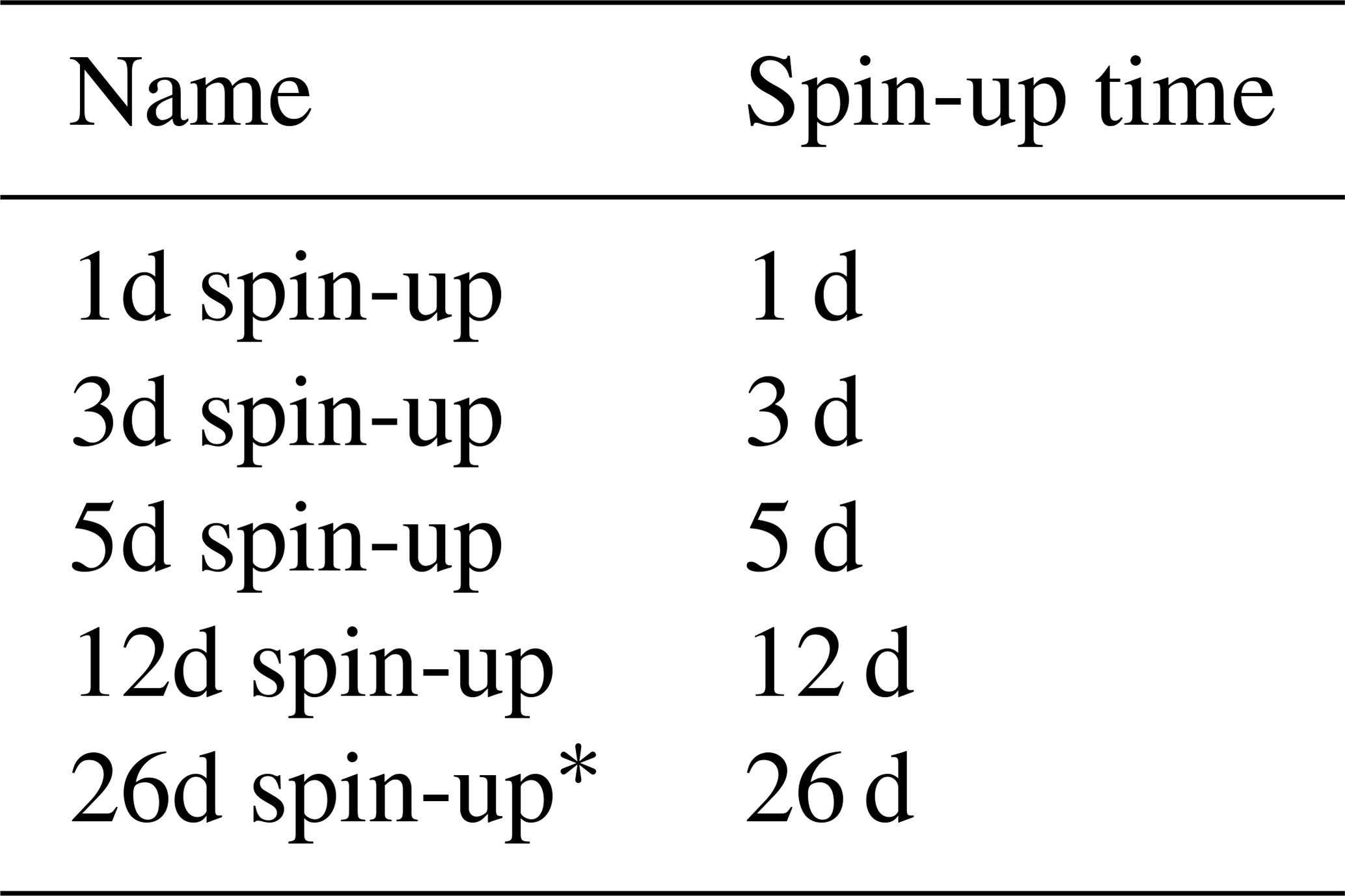
^*: a 26d spin-up period is used as the control (ctrl) in the snow experiments.

3.6 Prescribed snow cover experiments

During the October 2014 flood event, temperatures in the mountains were above freezing and the ground was bare. In other words, there was no layer of snow to act as a sponge and potentially affect the discharge. In a future warmer climate, however, rain-on-snow events are likely to increase, especially in mountainous areas of Norway (Vormoor et al., 2016). However, the potential impact of snow conditions on extreme flows is not well known. Therefore, we construct a series of hypothetical experiments for a primary check on this impact. The results can be helpful for filling this knowledge gap and dictating the flood-generation processes for Norway.

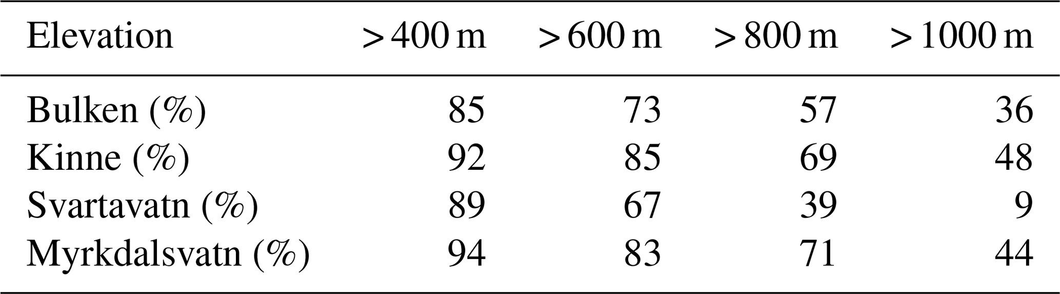
In this study, we perform two types of snow experiments: (1) different uniform snow depths are applied over the entire study area, i.e. 0.1, 0.5, 1 and 2 m, and (2) 1 m of snow is imposed above certain elevations, i.e. 400, 600 and 800 m a.s.l. (above sea level). The experiments are all performed with the calibrated parameter set. More details can be found in Table 3. We are mainly interested in evaluating the precipitation–snowmelt timing and snowmelt augmentation of the peak flow, if any exists. Therefore, we apply the prescribed snow cover fields in the restart file on the 25 October 2014, which is from the 26 d spin-up experiment. The area–elevation distribution in the four selected catchments is shown in Table 4. The Kinne and Myrkdalsvatn catchments are dominated by higher elevations with 48 % and 44 % of the area above 1000 m a.s.l. respectively, compared with 36 % and 9 % for the Bulken and Svartavatn catchments respectively (Table 4).

Table 3 Overview of the pre-existing snow cover experiments. All experiments are performed from 25 to 31 October, based on the 26 d spin-up simulation with the calibrated parameter set.

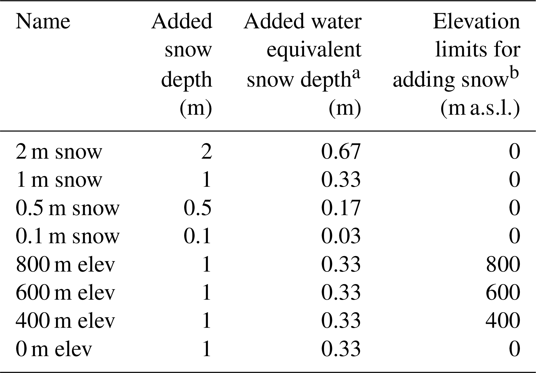
^a The snow density is assumed to be 300 kg m⁻³. ^b The elevation limit for adding snow is 0 m, which means that snow is added over the whole catchment area.

Table 4 Percentage of the catchment area of each of the four catchments at defined elevations.

4 Results

4.1 WRF-Hydro discharge calibration

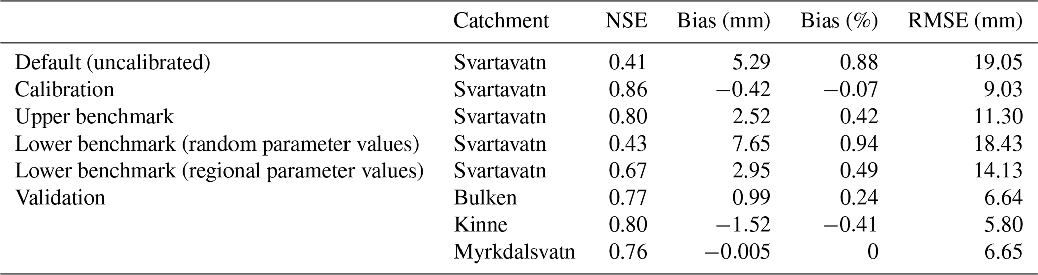
As calibration is computationally demanding, we calibrate WRF-Hydro based on the discharge of Svartavatn, which is the smallest catchment in the study region. The three remaining catchments are used for model validation. The calibration and validation results are shown in Table 5. The Nash–Sutcliffe efficiency coefficient (NSE) of daily discharge increases from 0.41 to 0.86, whereas the bias and RMSE decrease from 5.29 mm (0.88 %) to −0.42 mm (−0.07 %) and from 19.05 to 9.03 mm respectively. This indicates that the calibration greatly improves the representation of discharge over Svartavatn. The NSE values are 0.77, 0.80 and 0.76 for Bulken, Kinne and Myrkdalsvatn respectively, which are satisfactory, although they are slightly lower than the NSE value of 0.86 from Svartavatn. The infiltration parameters (refdk and refkdt) and the Manning routing coefficients (mn01) are calibrated using the PEST auto-calibration approach and are found to be $\mathrm{3.82}\times {\mathrm{10}}^{-\mathrm{6}}$, 0.63 and 0.18 respectively. The correlation coefficient values of mn01 and refdk, mn01 and refkdt, and refdk and refkdt are −0.23, −0.16 and 0.90 respectively. We can see that there is a high correlation between the refdk and refkdt infiltration parameters. Figure 3 shows the daily observed discharge (black line) and simulated WRF-Hydro discharge from four study basins using various refkdt values for the extreme event between 23 and 31 October 2014. It can be seen that WRF-Hydro is sensitive to the refkdt infiltration parameter and that the uncertainty of the peak flow is related to the parameters' uncertainties. The peak discharge decreases from 717, 309, 83 and 102 m³ s⁻¹ with a refkdt value of 0.2 to 698, 217, 81 and 85 m³ s⁻¹ with a refkdt value of 2.0 for the Bulken, Kinne, Svartavatn and Myrkdalsvatn basins respectively. An increase in refkdt in WRF-Hydro modelling leads to a decrease in peak flow and a slower recession limb in the hydrograph.

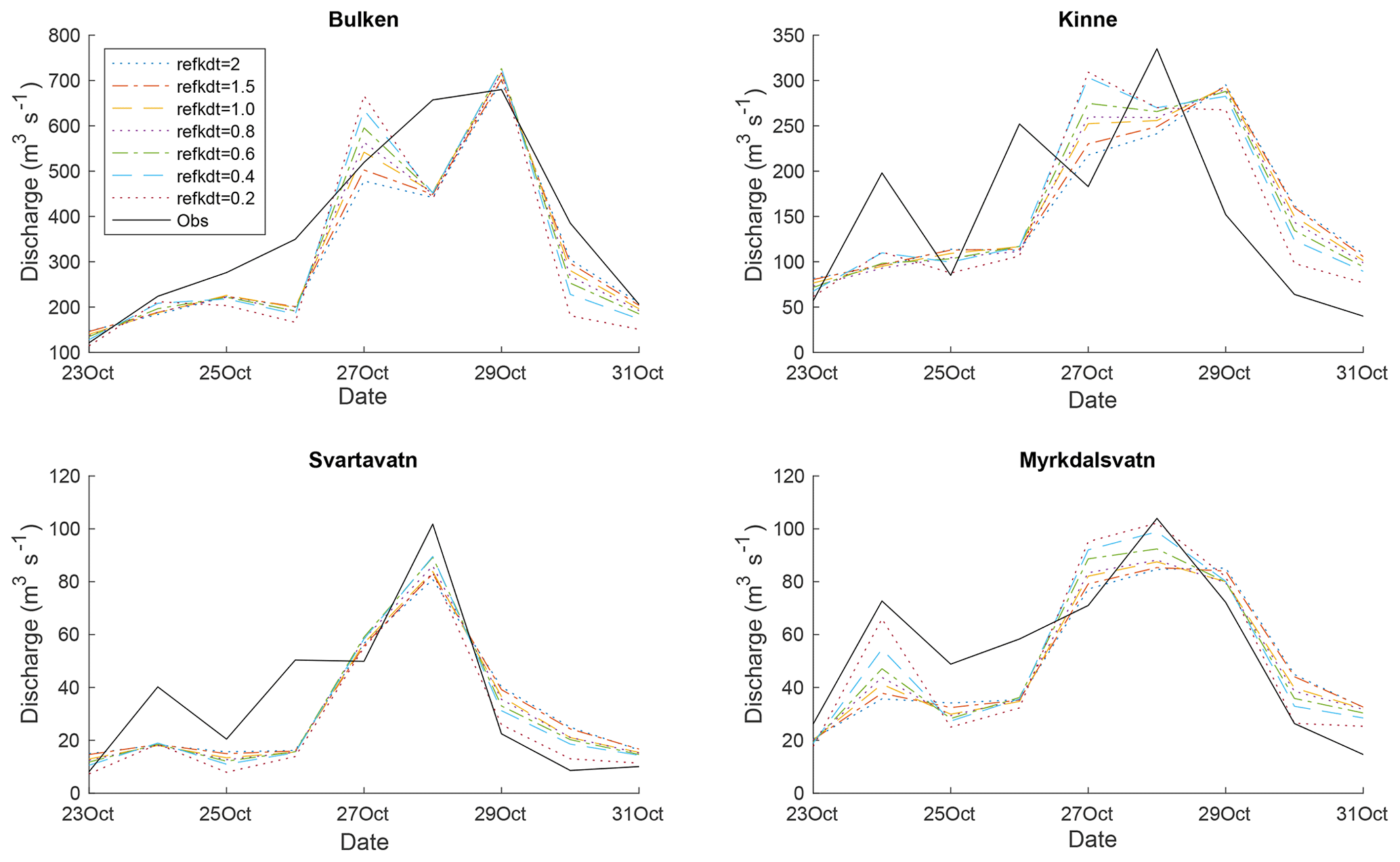
Figure 3 Hydrographs of daily observed discharge (Obs) and simulated WRF-Hydro discharge from four study basins using various refkdt values for the extreme event between 23 and 31 October 2014.

Table 5 WRF-Hydro uncalibrated, calibrated and validated results with model efficiency values for different benchmarks.

The daily observed discharge and simulated discharge based on the calibrated parameter set and the uncalibrated parameter set from the four study catchments are plotted in Fig. 4. The hydrographs show that the calibrated runs capture the peak timing and magnitude well in all four catchments and that calibration markedly improves these features. The water balance of the four study catchments is shown in Table 6, highlighting that the discharge at the four study catchments is driven by intense rainfall, and the impact of evapotranspiration (ET) and the changes in snow depth water equivalent and soil moisture are minor. ET is small for all of the catchments. This is due to the low temperatures at the end of October in western Norway, which is located very close to the Arctic Circle and is dominated by mountainous terrain (Engeland et al., 2004).

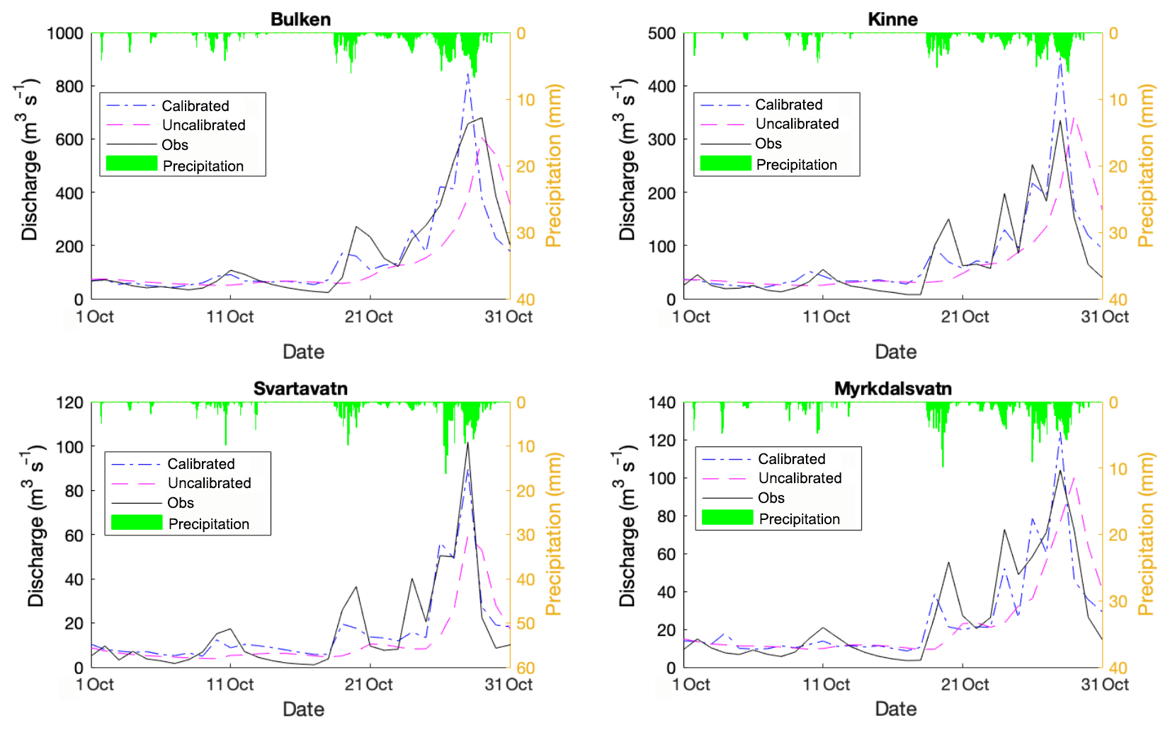
Figure 4 Hydrographs of daily observed discharge (Obs) and simulated discharge with calibrated parameters (Calibrated) and uncalibrated parameters (Uncalibrated) as well as precipitation from 1 to 31 October 2014.

Table 6 The water balance of the four study catchments from 25 to 31 October 2014, based on the calibrated parameter sets (values are given in millimetres).

4.2 Benchmark evaluation

Furthermore, the benchmark model efficiencies are also shown in Table 5. Daily precipitation, temperature and potential evapotranspiration from WRF are used as input for the HBV light model in order to calculate benchmarks. For the upper benchmark (i.e. using calibrated parameters), the calibrated HBV model efficiency (R_upper) of the Svartavatn basin is 0.80. For the lower benchmarks, the HBV model efficiency is 0.43 when calculated from random parameters (R_{lower∕random}) and is 0.67 when calculated from regionalized parameter sets based on three nearby catchments (R_{lower∕regional}). The bias and RMSE values are −0.42 mm (−0.07 %) and 9.03 mm from calibrated WRF-Hydro, 2.52 mm (0.42 %) and 11.3 mm from the upper benchmark, and 7.65 mm (0.94 %)∕2.95 mm (0.49 %) and 18.43 mm∕14.13 mm from two lower benchmarks ($R_{\mathrm{lower}/\mathrm{random}}/R_{\mathrm{lower}/\mathrm{regional}}$). These results show that the calibrated WRF-Hydro model NSE value of 0.86 is well above the upper benchmark (0.80). Moreover, the calibrated WRF-Hydro has both a lower bias and a smaller RMSE than the upper benchmark. Despite this encouraging result, some care must be taken in the interpretation due to uncertainty in the input data for the HBV simulation, which is caused by a lack of long-term averaged monthly meteorological forcing.

4.3 Precipitation evaluation

The accumulated precipitation from 23 October at 06:00 UTC to 31 October at 06:00 UTC is shown in Fig. 5. The ctrl simulation (see Table 3) is shown using coloured contours, and the observed values are shown using coloured squares (circles) for the HOBO rain gauge (meteorological) observational network. The observed precipitation amounts correspond well to the model simulation at the majority of the stations. The spatial variability is large in the complex terrain with several areas receiving close to 500 mm precipitation and some areas less than 100 mm during the week.

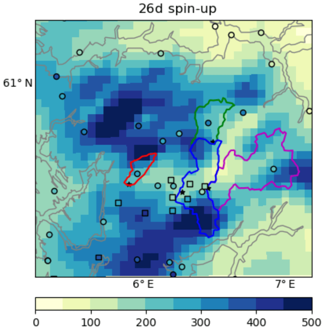
Figure 5 Accumulated precipitation (mm) between 23 and 31 October from the 26 d spin up ctrl simulation. The catchments are contoured using colours that correspond to those used in Fig. 9. Squares and circles are observational values from the HOBO network and the meteorological network respectively.

The temporal evolution of simulated precipitation at monitoring locations is shown in Fig. 6. Observational stations are depicted in Fig. 6a and the simulated precipitation interpolated from the four nearest grid points in the ctrl simulation is shown in Fig. 6b. Daily precipitation values are shown using diamonds, whereas hourly values are shown using continuous lines. The temporal evolution is generally well reproduced by the simulation, as is the timing of periods of precipitation.

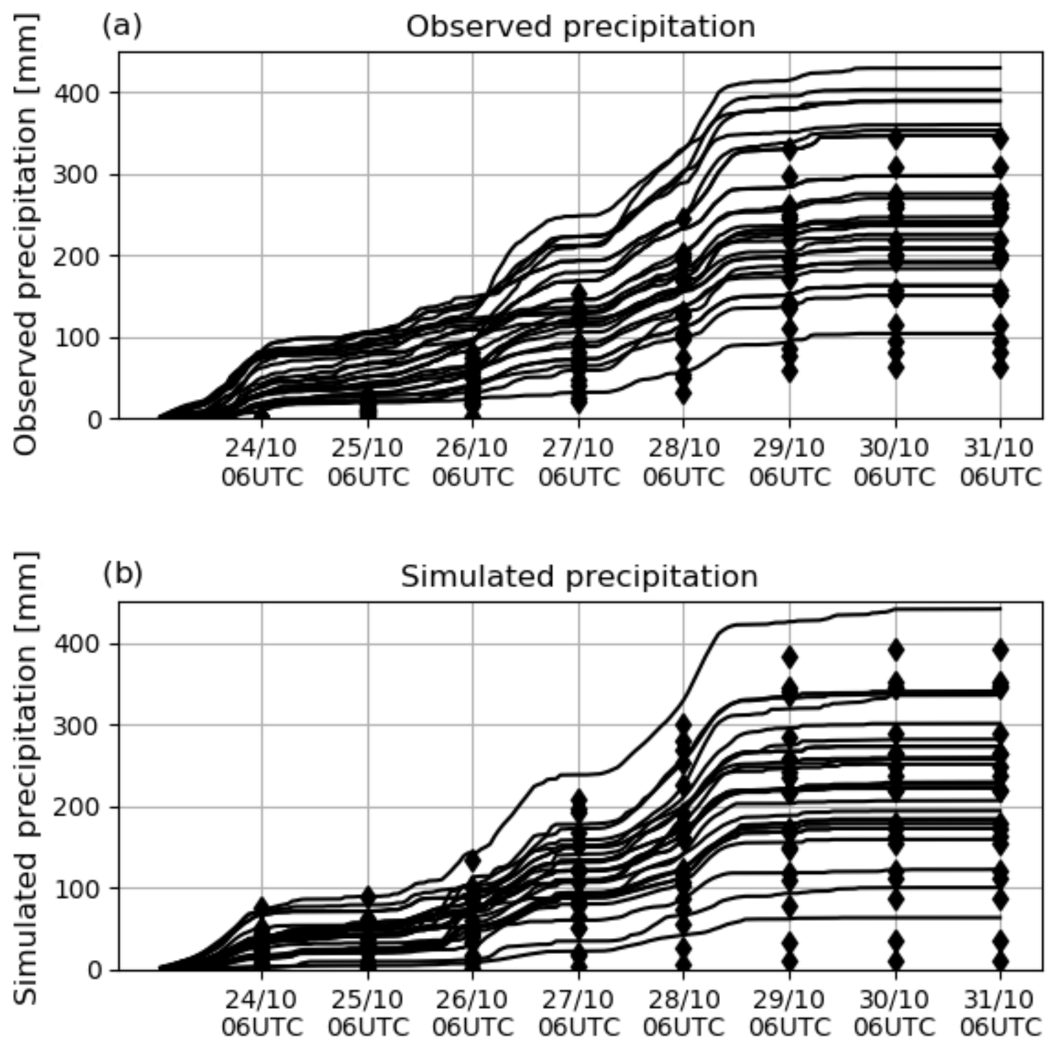
Figure 6 Accumulated precipitation from 23 October at 06:00 UTC to 31 October at 06:00 UTC (a) at observation stations in the area and (b) interpolated from the four nearest grid points to the equivalent station position in the 26 d spin up simulation. The lines represent stations with hourly precipitation measurements, whereas the diamonds represent stations with daily precipitation values. The same notation is used in panel (b), although the model output enables a higher temporal resolution at the daily station positions.

4.4 Sensitivity to spin-up time

Five different spin-up times are investigated in order to analyse the sensitivity of precipitation and discharge to the initial conditions (see list in Table 3). The same calibrated parameter set is used for all of the spin-up experiments.

During this event, the western coast of Norway was exposed to a considerable amount of precipitation within a 4 d period. Furthermore, the soil was already saturated after a wet October, as can be seen in Fig. 7: panel (a) shows the catchment-averaged total soil moisture of the four catchments in the ctrl experiment (26d spin-up), panel (b) shows the averaged total soil moisture on 24 October, panel (c) shows the difference in soil moisture between the 1d spin-up and the ctrl, and panel (d) shows the difference in soil moisture between the 12d spin-up and the ctrl. Figure 7 indicates the sensitivity of soil moisture to spin-up time, although the differences are fairly small (−10 to 10 mm, which is around ±1 %). The difference between experiments is more clearly highlighted in Fig. 8, which shows the evolution of basin-averaged soil moisture during the period from 23 to 31 October. The soil moisture on the first day clearly differs between spin-up times in all catchments. More specifically, the soil moisture on 23 October increases with spin-up time, which indicates that runs with a short spin-up have a much drier soil that can absorb additional precipitation during the initial phase of the event (i.e. 23–25 October). In general, the soil becomes slightly wetter with increased spin-up time. A total of 2–3 d after initialization, the soil is saturated irrespective of the spin-up time. This is likely due to the relatively shallow soil depth in the mountainous region of southern Norway.

Figure 7 (a) Temporal evolution of the total column soil moisture averaged in the catchments (ctrl simulation). (b) The averaged total column soil moisture on 24 October. (c) The soil moisture differences between the 1 d spin-up and the control simulation. (d) The soil moisture difference between the 12 d spin-up and the control simulation.

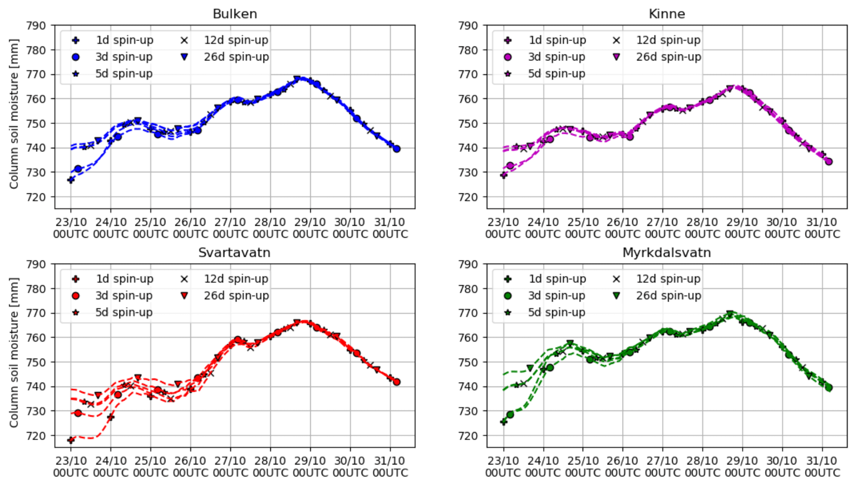
Figure 8 The basin-averaged simulated soil moisture with different spin-up times, including 1 d (1d spin-up), 3 d (3d spin-up), 5 d (5d spin-up), 12 d (12d spin-up) and 26 d (26d spin-up) for the flooding events between 23 and 31 October 2014.

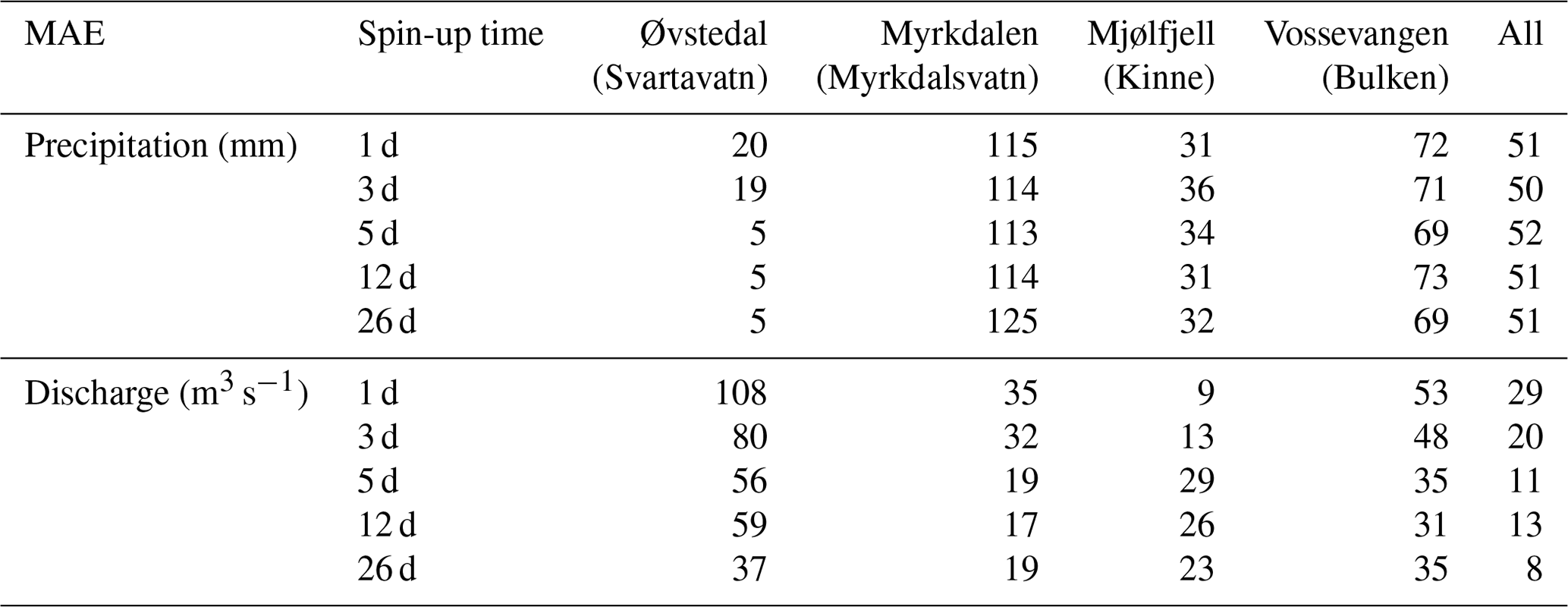
In addition, we evaluate the temporal evolution of the precipitation for the spin-up experiments. Figure 9 shows the accumulated precipitation interpolated from the four nearest grid points to the following four rain gauge stations: Øvstedal, Myrkdalen, Mjølfjell and Vossevangen. These are the official meteorological observational stations located in the Svartavatn, Myrkdalen, Kinne and Bulken catchments respectively. The precipitation sensitivity to spin-up time is low in all catchments. At Øvstedal and Mjølfjell the precipitation is reproduced well, whereas the remaining two stations are somewhat biased. The model seems to be unable to catch the finer-scale phenomena completely with a 3 km grid resolution, especially over a small complex catchment such as Myrkdalsvatn. This could be partly due to the combination of highly complex terrain and interactions with the Sognefjord, just to the north, which are missing in the simulation. Table 7 provides additional evidence of this, showing the mean absolute error (MAE) in the total accumulated precipitation and discharge. The differences in the MAE of precipitation between the spin-up experiments are negligible; we believe this is due to the large-scale nudging in the outer domain. Furthermore, there is no decrease in the precipitation MAE with an increase in spin-up time for any of the stations except Øvstedal. The averaged MAE of precipitation at all 54 observational stations in the area is around 50 mm. This suggests that the model, even at 3 km grid spacing, struggles to fully reproduce the local-scale orographic effects in the complex terrain around Voss and Myrkdalen. A previous study in the high mountains of Asia suggested that a sub-kilometre-scale grid is needed to accurately estimate truly local meteorological variability (Bonekamp et al., 2018).

Table 7 Mean absolute error of precipitation and discharge compared with observations from simulations (23–31 October) with different spin-up times. The accumulated precipitation was interpolated from the four nearest grid points to Øvstedal, Myrkdalen, Mjølfjell, Vossevangen and “All”, the latter of which refers to the 54 observational stations available in the area.

The temporal evolution of streamflow over the four catchments is shown in Fig. 10, which displays the daily hydrograph of discharge for the four catchments as a product of different spin-up experiments. We want to capture this flood event completely in our spin-up experiment, so we evaluate the period from 23 to 31 October. From the results, we can see that the precipitation amount and timing do not differ significantly between spin-up times in any of the catchments. However, the discharge at the pre-flood phase, which is from 23 to 24 October, is more sensitive to the spin-up time. For Svartavatn, this sensitive phase even extends to the 26 October. This is because the initial condition of soil moisture affects the overland flow that dominates the discharge of this catchment (see Fig. 8). The pre-flood discharge moves closer to the observed discharge when we increase the spin-up time from 1 to 26 d, which confirms the soil moisture feedbacks from different spin-up time experiments in Fig. 8. In general, the peak flows are overestimated compared with the observations, except in the Svartavatn catchment. This is because we only calibrated the model in Svartavatn, and then used this calibrated parameter set in the simulation for the other three catchments, which, perforce, have poorer performance than the Svartavatn catchment.

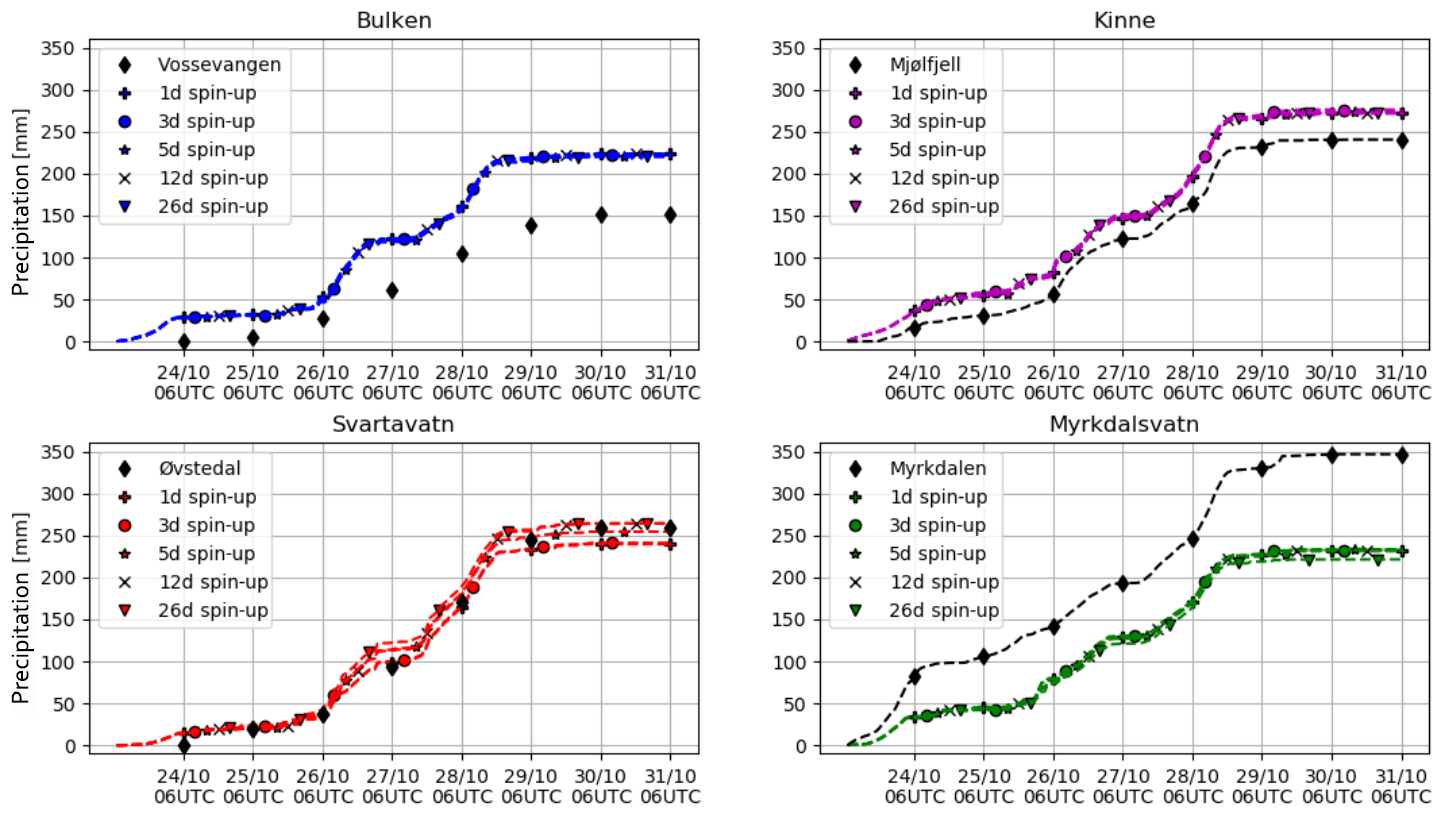
Figure 9 The accumulated precipitation from the simulations at the four nearest grid points to the Vossevangen (Bulken), Mjølfjell (Kinne), Myrkdalen (Myrkdalsvatn) and Øvstedal (Svartavatn) observational stations from the different spin-up time simulations, including 1 d (1d spin-up), 3 d (3d spin-up), 5 d (5d spin-up), 12 d (12d spin-up) and 26 d (26d spin-up) compared with the observational station within the catchment.

Figure 10 Daily observed streamflow (Obs) and simulated discharges as a product of different spin-up times, including 1 d (1d spin-up), 3 d (3d spin-up), 5 d (5d spin-up), 12 d (12d spin-up) and 26 d (26d spin-up) for the flooding events from 23 to 31 October 2014.

4.5 Sensitivity to prescribed snow cover

The dynamical modelling experiments of different snow conditions are based on the WRF-Hydro simulation with a 26 d spin-up, which is labelled as the control (ctrl) in the snow experiments (Table 2). In these experiments, the snow depth and the water equivalent snow depth are changed in the 25 October restart file and the simulations are restarted in offline mode. An overview of the snow experiments is presented in Table 3. In summary, one set of experiments tests the sensitivity to varying snow depths, whereas the other set of experiments tests the sensitivity to snow elevation. The temporal evolution of catchment-averaged SWE is shown in Figs. 11 and 12. A decline throughout the simulation period is shown for all catchments. The experiments with the 0.5, 1 and 2 m snow depths have similar snowmelt behaviour from 25 to 28 October. The snowmelt stops in all of the snow experiments after 29 October due to a drop in both rainfall and temperature (below 273 K), which can be seen in Fig. 11. More detailed information on the total snowmelt from 25 to 31 October as a product of the different snow experiments is given in Table 8. From Table 8, we can see that, except for the 0.1 m snow depth experiment where the added snow quickly melts away, the results from the 0.5, 1.0 and 2.0 m snow depth experiments are fairly similar: the total water equivalent snowmelt is 14–16 cm in Svartavatn, 11–12 cm in Myrkdalsvatn, 11–12 cm in Kinne and 12–13 cm in Bulken. This is because the limit of melting snow is controlled by the temperature in the Noah LSM and a maximum of around 0.5 m of snow will be melted away in this case. For the snow elevation experiment where 1 m of snow was added above the given ground elevation, the response is a result of the elevation of the catchments. In Kinne and Myrkdalsvatn there is little variation, around 8–11 cm of SWE melts. Their average catchment height is so high that there is only a small difference in total SWE between the experiments, leading to a similar response. For Svartavatn and Bulken, the situation is different. The total SWE in the catchments varies between the experiments due to the lower catchment elevation; hence, the resultant SWE melting varies between 2 and 16 cm for Svartavatn and between 4 and 12 cm for Bulken.

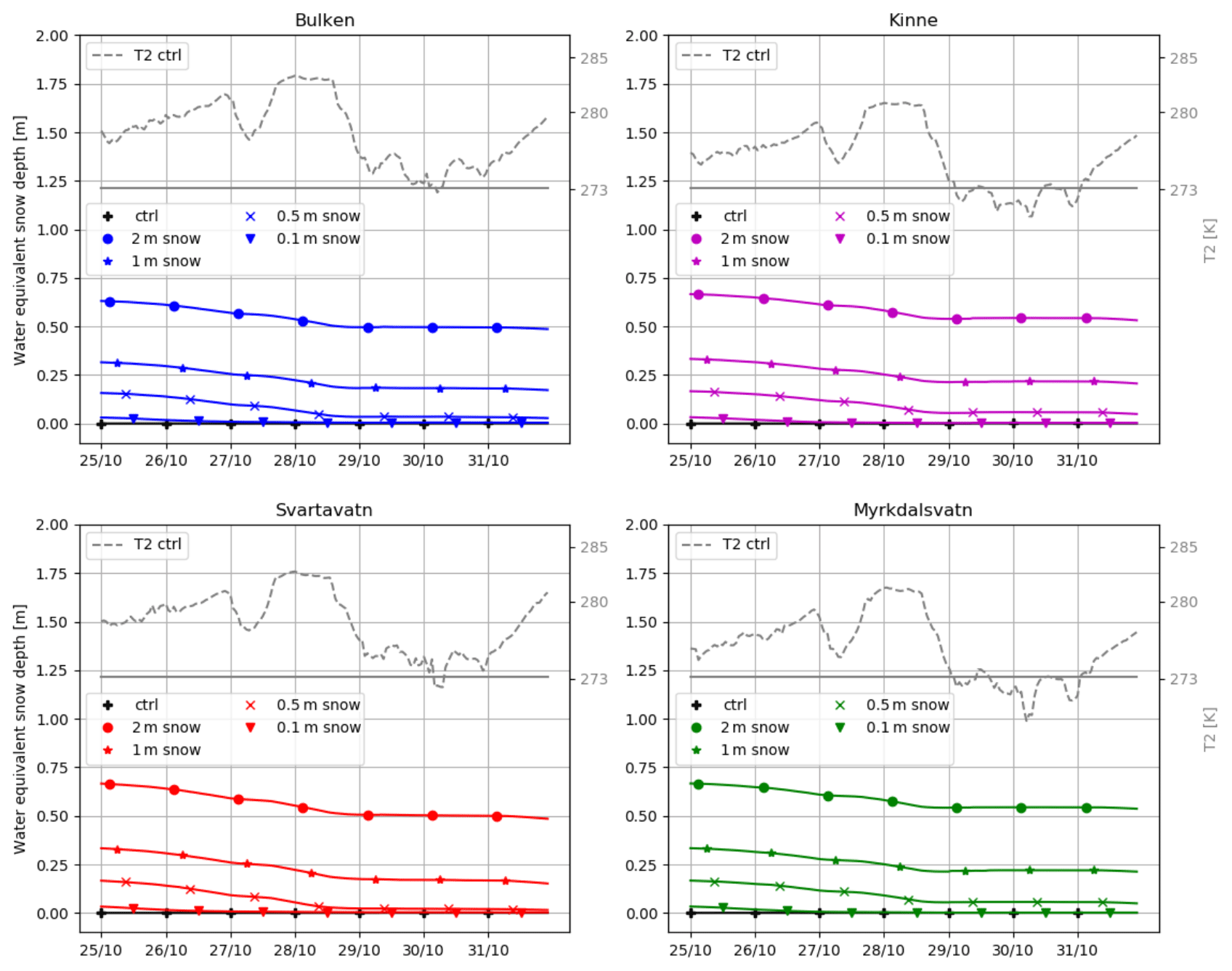
Figure 11 Catchment-averaged hourly snow water equivalents from the 3 km WRF-Hydro simulation for the snow sensitivity experiments, including 2 m added snow depth (2 m snow), 1 m added snow depth (1 m snow), 0.5 m added snow depth (0.5 m snow), 0.1 m added snow depth (0.1 m snow), and the catchment-averaged hourly snow water equivalent (ctrl) and surface temperature (T2) from the control simulation of the 26 d spin-up.

Table 8 The total water equivalent snow depth change between 25 and 31 October as a product of the different pre-existing snow cover experiments in the four study catchments.

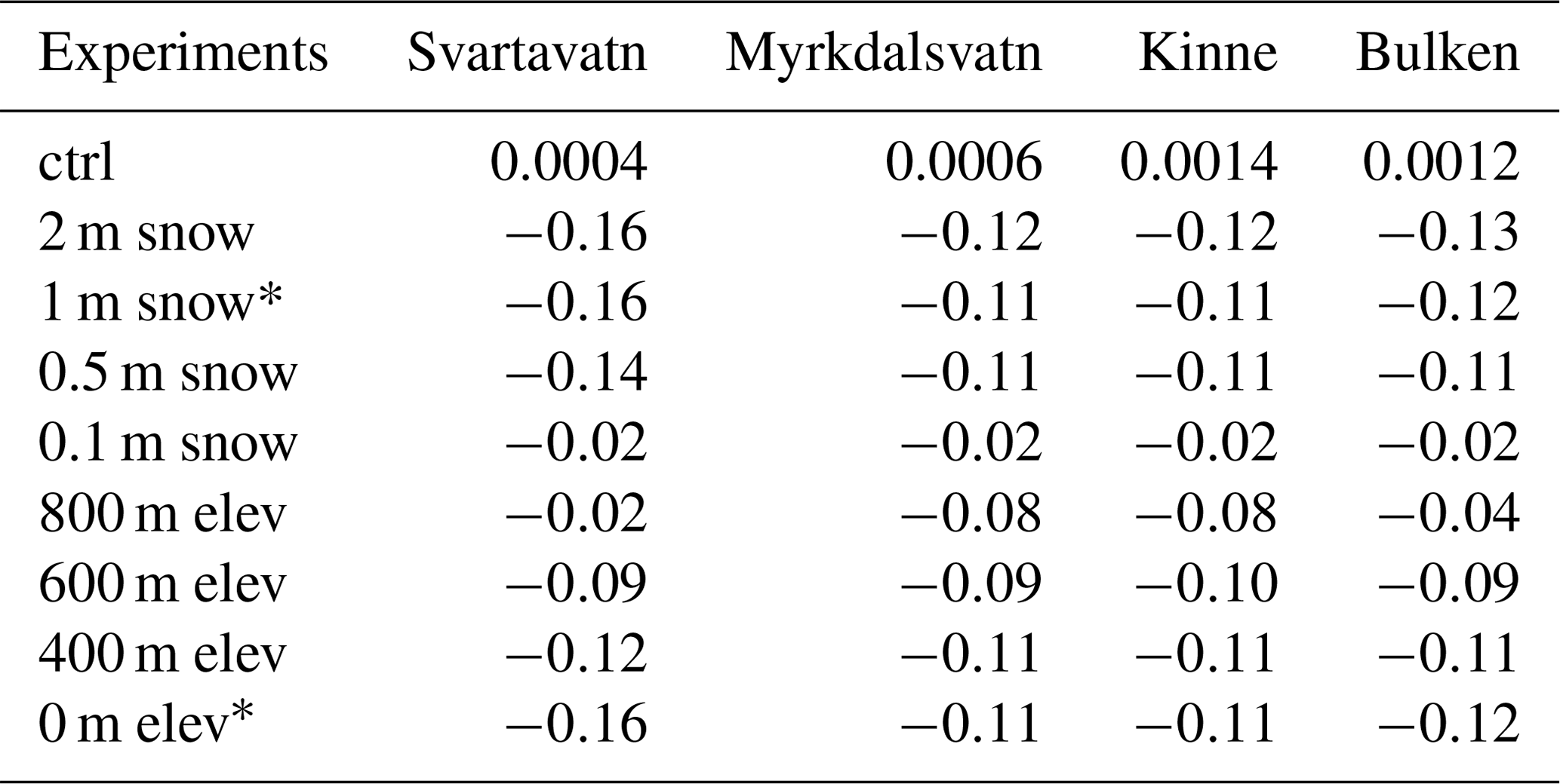
^*: the 1 m snow and 0 m elev experiments refer to the same experiment.

Figure 13 shows the hydrograph of hourly discharge for the experiments where snow depth is modified uniformly over the entire area. From both Figs. 11 and 13, we can see that the difference in melt between the shallowest and deepest snow depths is less than 2 cm, which suggests that snow depths beyond 0.5 m did not contribute markedly to increased discharge. The main contribution from the additional snow is to enhance the peak discharge in all of the catchments. Moreover, the contribution from melting snow is mostly confined to periods of precipitation, which also coincides with higher temperatures. The fact that snow depths above 0.5 m have little impact suggests that rain-on-snow can melt 0.5 m of snow at most under these experimental conditions. The snowmelt discharge decreases after 29 October, which is preceded by a drop in both rainfall and surface temperature (below 273 K). It is worthwhile recalling that the Noah LSM has a simple bulk snow–soil–canopy layer model. Previous studies have noted that there was a positive bias in snow surface energy in the Noah LSM that resulted in an underestimation of snow water equivalent (SWE) and led to a reduced snow pack during winter as well as earlier snowmelt in spring (Jin and Miller, 2007; Jin and Wen, 2012; Niu et al., 2011). In our experiments, this positive bias in snow surface energy in the Noah LSM as well as energy from intense rainfall are probably used to melt snow directly; therefore, the warm snowpack does not retain any liquid water which can refreeze during the day before it runs away. In this case, we might see unrealistically high snowmelt, and the snowpack would not act like a sponge and retain part of the rainfall. All in all, the snow experiments show that intense precipitation coinciding with a higher temperature can result in up to 0.5 m of snowmelt, which contributes to the peak flow. However, more work needs to be carried out in the future with more sophisticated multi-layer snow models to confirm the behaviour observed in these idealized experiments.

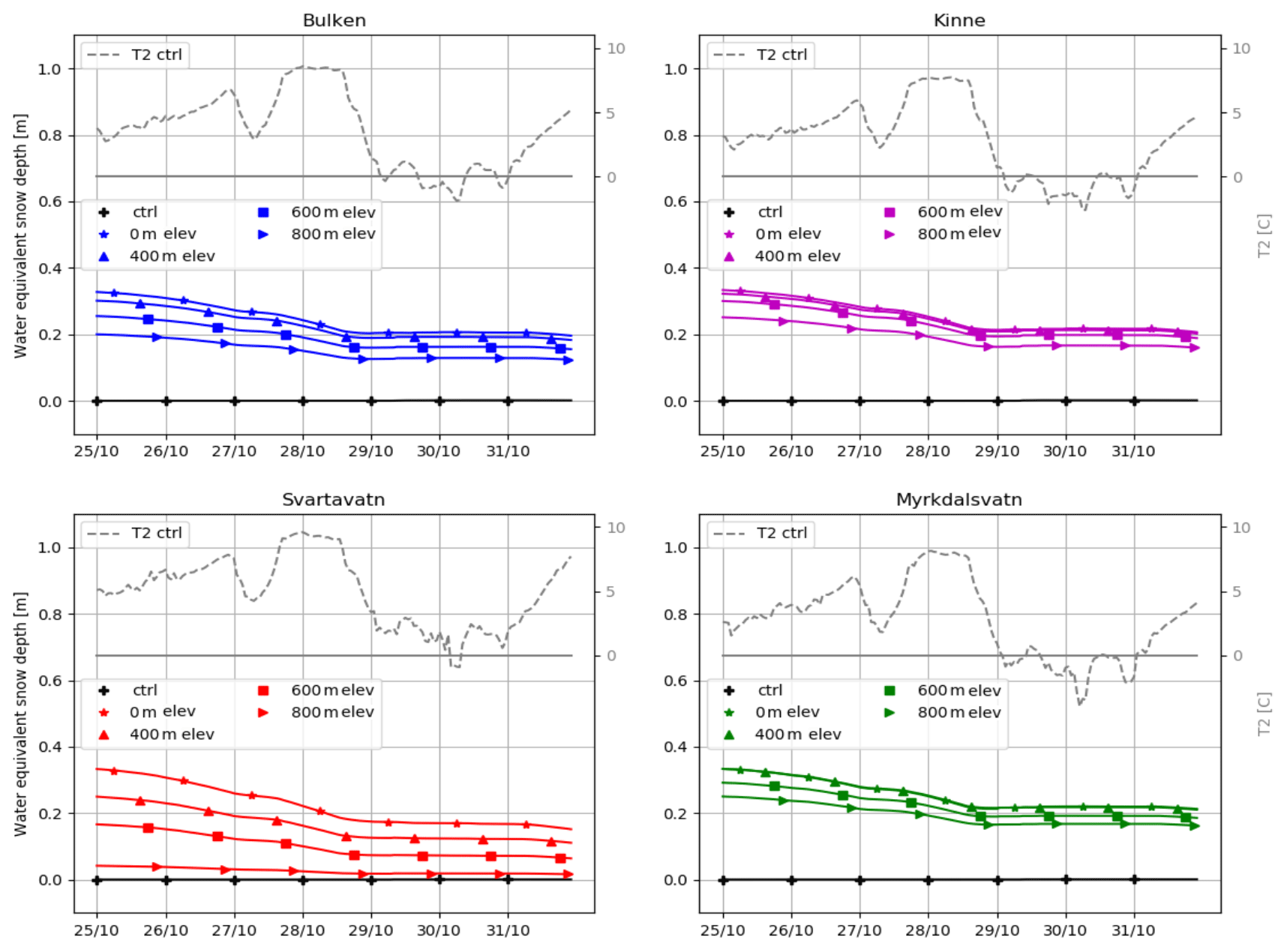
Figure 12 Catchment-averaged snow water equivalents from the 3 km WRF-Hydro simulation for the pre-existing snow cover sensitivity experiments, including 1 m added snow depth to the area where the elevation is above 0 m (0 m elev), 400 m (400 m elev), 600 m (600 m elev) and 800 m (800 m elev) based on the ctrl simulation (26 d spin-up) as well as the catchment-averaged hourly snow water equivalent (ctrl) and surface temperature (T2) from the control simulation of the 26 d spin-up.

The effects of varying snow cover by altitude on daily discharge are shown in Fig. 14. Here, we perform snow experiments where 1 m of snow is imposed above certain elevations, i.e. 400, 600 and 800 m. These prescribed snow covers are applied in the restart file on 25 October 2014, which is from the 26 d spin-up experiment with the calibrated parameter set. From Fig. 14, we can see that there are increases in snowmelt runoff with the elevation decreases from 800 to 0 m and that the differences in snowmelt runoff among different experiments vary in different catchments; for example, the snowmelt runoff from the 0 and 800 m experiments show a large difference in the Svartavatn catchment, whereas not much difference can be seen in the Kinne and Myrkdalsvatn catchments. This is because varying the prescribed snow cover by elevation has a greater influence on the lower catchments, such as Svartavatn (with 61 % of the area below 800 m), than on the higher catchments, such as Kinne and Myrkdalsvatn (with 69 % and 71 % above 800 m respectively). A more detailed quantitative estimate of the total water equivalent snow depth change from 25 to 31 October under different prescribed snow cover experimental conditions is given in Table 8. It confirms the results in Figs. 11 and 12, with the first 0.5 m of the snowpack contributing the to the snowmelt. In addition, there is a greater SWE decrease in the lower-elevation catchment of Svartavatn (i.e. −0.16 m in the 1 m of added snow experiment) than in the Kinne and Myrkdalsvatn catchments (i.e. −0.11 m in the 1 m of added snow experiment), which are dominated by higher elevations.

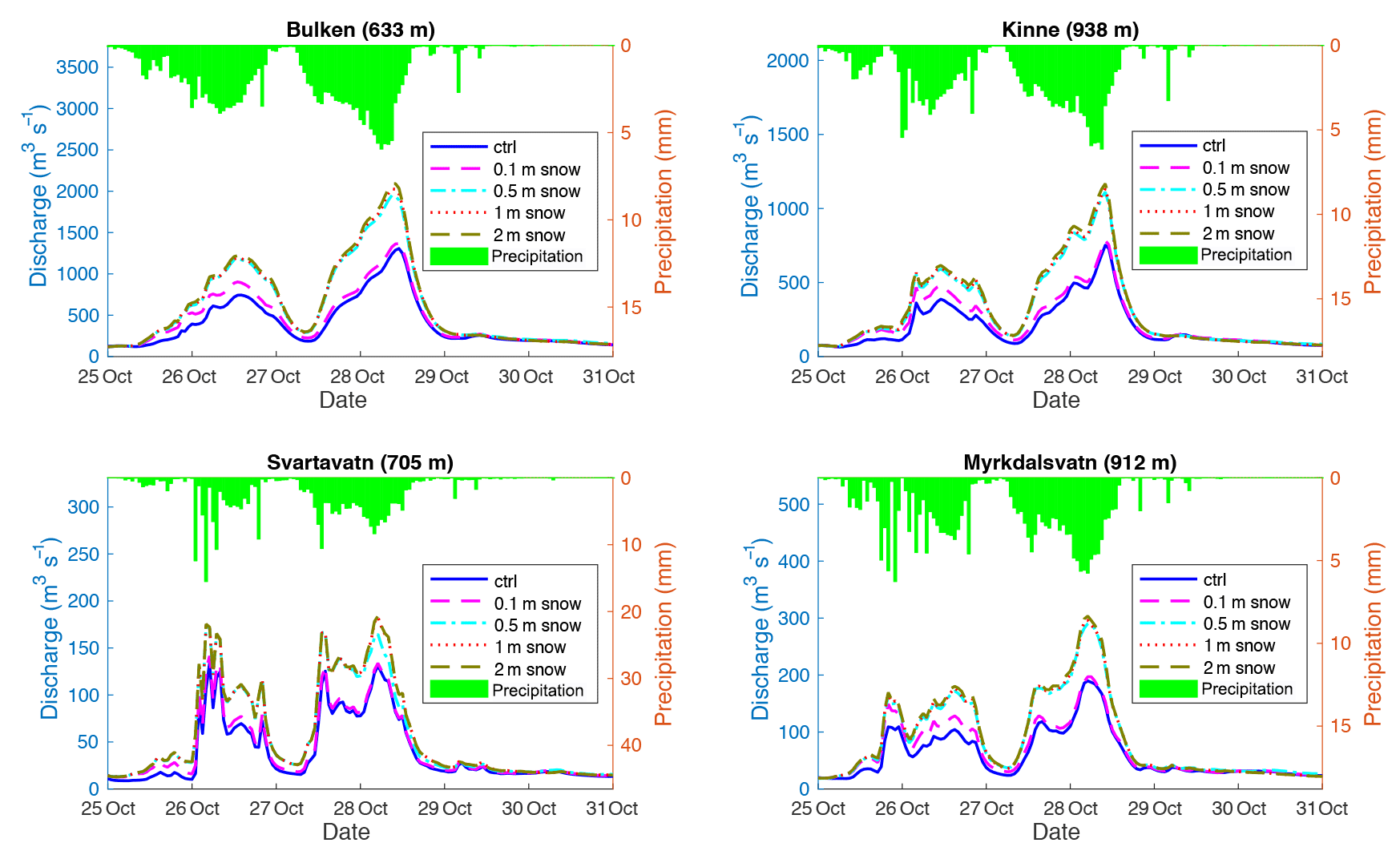
Figure 13 Hourly simulated discharge from 25 to 31 October from different added snow depth experiments – 0.5, 1 and 2 m of added snow and the control simulation from the 26 d spin-up without added snow (ctrl). (The mean elevations of the four basins are given in parentheses in the panel headings.)

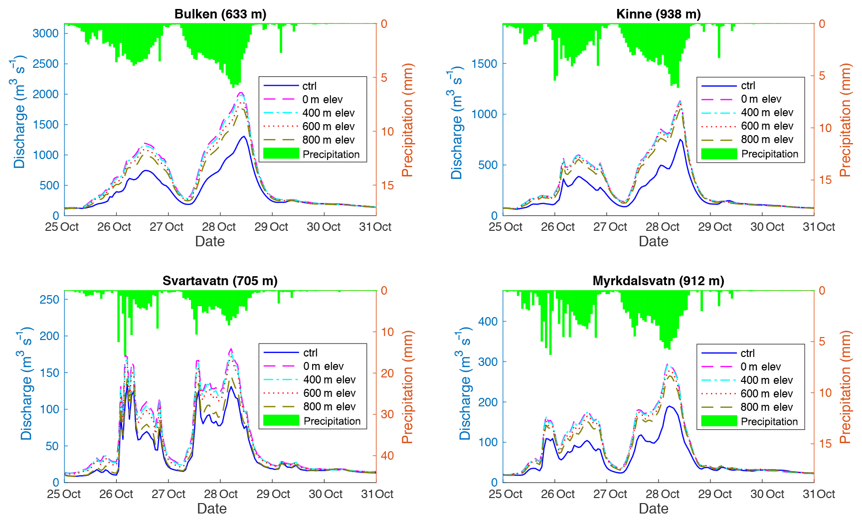
Figure 14 Hourly simulated discharge from 25 to 31 October from the control simulation (ctrl) and the different experiments with 1 m of added snow depth on areas with elevations above 0, 400, 600 and 800 m. (The mean elevations of the four basins are given in parentheses in the panel headings.)

5 Discussion

Precipitation patterns in Norway vary spatially and are highly affected by the complex topography. More specifically, there is a strong west–east gradient of precipitation, with decreasing amounts as we move eastwards across the mountain range (Dyrrdal, 2015). To represent the interaction between the atmosphere and the complex terrain realistically there is a need for high spatial resolution in models. For example, for the episode under investigation here, Pontoppidan et al. (2017) showed that a 3 km grid scale represented the precipitation distribution better than an equivalent simulation with 9 km grid spacing, which lacked the observed spatial variability and was unable to show dynamical features like gravity waves. Furthermore, a recent study by Magnusson et al. (2019) found that the grid resolution is important in energy-balanced snow models and that the scale error increases with sub-grid topographic variability. They also suggested that the best option for snow models is to run at the highest possible resolution and that any upscaling can bring large regional errors because of model nonlinearities. The results from our study confirmed that convection-permitting simulations reasonably fit the requirements of hydrological processes determining flood events in western Norway and address them in a realistic manner.

Most of the precipitation in Norway is frontal, caused by large-scale cyclone activity in the North Atlantic (Heikkilä et al., 2011). In the west coast region, extreme precipitation occurs in autumn and winter, which is dominated by orography and frontal systems (Dyrrdal, 2015). In eastern Norway, where the mountain ranges are located, the annual precipitation is less than in the west but with the highest amounts occurring near the steepest surface slopes in winter and fall (Andersen, 1972). In southeastern Norway, however, intense precipitation is dominated by convective precipitation in summer. Norway, despite its high latitude, has a diverse range of climates, including northern Arctic, central alpine and southern maritime, and can exhibit an equally wide range of snow regimes (Pall et al., 2019). The role of snowmelt and rainfall is highly relevant for the seasonal flood regimes (Barnett et al., 2005; Vormoor et al., 2016). For example, south-central Norway has an alpine climate, which receives large amounts of precipitation as snowfall, approximately 30 % (Saloranta, 2012), and has high discharge during spring and early summer due to snowmelt. Southwestern Norway has a maritime climate and the highest precipitation occurs in fall and winter, which often results in flood events (Vormoor et al., 2016). From the results of the study, we can see that the snow feedback to river flow depends on which snow regime the region experiences, i.e. little or no snow (ctrl, 0.1 m of snow), a lot of snow (1.0 or 2.0 m of snow) or somewhere in between (0.5 m of snow). According to previous studies of the current climate, snow cover above 800 m is present for over 200 d of the year in southern Norway (Hanssen-Bauer et al., 2015), and the observed median snow depth in Norway varies from 0.1 to 0.5 m during October–May (1957–2011) (Saloranta, 2012). In some regions of southern Norway, the snow depth can be up to 2–3 m during the late winter (Andreassen and Oerlemans, 2009). Furthermore, Pall et al. (2019) constructed a rain-on-snow climatology using a 1 km gridded observation data (from 1961 to 1990) and found that the average monthly count of daily rain-on-snow events varies from two to four during winter–spring in southern Norway. Under the impact of climate change, the snowpack distribution (both temporal and spatial) in Norway will change. In general, snowmelt floods will decrease in Norway, while winter precipitation will increase, which may also lead to larger snow storage, e.g. in mountainous areas in eastern Norway (Hanssen-Bauer et al., 2015). Meanwhile, other studies have also shown that general increases in both precipitation and temperature (especially warmer winters) in Norway will intensify the risk of rain-on-snow events in certain regions and seasons. Such events can be major triggers of hazards, i.e. floods and landslides, in the country (Hansen et al., 2014; Pall et al., 2019). The regional patterns of increases and decreases in flood events (both frequency and magnitude) reflect the balance between the different and sometimes counteracting processes, e.g. snowpack dynamics, snowfall versus rainfall.

6 Conclusions

In this study, a dynamical hydrometeorological modelling system (WRF-Hydro) was employed to reproduce an extreme weather event in a region characterized by complex terrain. A nested WRF atmospheric model, run at convection-permitting scales, was used to reproduce the meteorological event and provide precipitation forcing for a distributed hydrological model over a small domain encompassing four study catchments affected by extreme flooding. A 3 km grid spacing was used for the WRF atmosphere and land surface, whereas a 300 m grid spacing was used for the WRF-Hydro river routing. An auto-calibration tool was used for the WRF-Hydro model calibration based on the daily discharge at Svartavatn, which is the smallest of the four catchments. The simulation of high-resolution precipitation and discharge was assessed based on observational data sets. Furthermore, the sensitivity of the results to the spin-up time and snow depth was investigated.

The results showed that the precipitation from the 3 km simulation generally agreed well with the rain gauges both in terms of temporal evolution and spatial variability, although it underestimated the precipitation in the highly complex terrain around Myrkdalen. This underestimation could be due to a combination of the locally complex topography and the proximity to the Sognefjord (only 15 km away). This large, but narrow body of water, and its many offshoots, was not well-resolved by the modelling system.

The auto-calibration greatly improved the model performance with the NSE increasing from 0.41 to 0.86 and the bias and RMSE decreasing from 5.29 and 19.05 to −0.42 and 9.03 mm respectively. The modelling system captured peak flow volumes and timing well after model calibration. In addition, WRF-Hydro runoff performance depended on some highly sensitive parameters (e.g. the infiltration parameter and the Manning routing coefficients).

In comparison with the benchmarks, the calibrated WRF-Hydro NSE value (0.86) was higher than the upper benchmark from the HBV light model (0.80). This might be due a lack of long-term input data (e.g. averaged monthly potential evapotranspiration). The implication of this was that WRF-Hydro might perform as well or even better than a simpler conceptual hydrological model, especially for ungauged basins or observation-scarce regions.

The precipitation simulation was not overly sensitive to spin-up time. We found that mean absolute errors of precipitation were very similar given different spin-up times. This could be due, in part, to the decision to nudge the atmospheric flow to match that large-scale reanalysis. Discharge simulations were slightly more sensitive to the spin-up time due to the impact of soil moisture, especially during the pre-peak phase. We found that a spin-up time of 26 d give the lowest MAE of precipitation and discharge compared with the other smaller periods.

SWE melt from 25 to 31 October was consistently around 10–16 cm for the uniform snow depth experiments (0.5–2 m). The results also showed that melting snow contributes most to discharge during rainy and peak flow periods. This indicated that snow cover intensified the extreme discharge instead of acting as a sponge in this study, which suggested that future rain-on-snow events might potentially result in a higher flood risk. However, more sophisticated snow models and targeted experiments should be conducted to confirm this speculation.

Our results increased confidence in the performance of WRF-Hydro for simulating extreme hydrometeorological events over complex terrain. Furthermore, they demonstrated the importance of model calibration and reasonably accurate land surface initial conditions for simulating discharge, especially for peak flow. The snow experiments suggested that rain-on-snow events under warmer conditions might contribute to an increase in flood magnitudes in Norway, due to projected increases in extreme precipitation (Lawrence, 2016). However, targeted experiments on the changing risks associated with future rain-on-snow events are needed to confirm this possibility.