the Creative Commons Attribution 4.0 License.
the Creative Commons Attribution 4.0 License.
 | 17 Feb 2020
Freshwater pearl mussels from northern Sweden serve as long-term, high-resolution stream water isotope recorders
Bernd R. Schöne
Aliona E. Meret
Sven M. Baier
Jens Fiebig
Jan Esper
Jeffrey McDonnell
Laurent Pfister
The stable isotope composition of lacustrine sediments is routinely used to infer Late Holocene changes in precipitation over Scandinavia and, ultimately, atmospheric circulation dynamics in the North Atlantic realm. However, such archives only provide a low temporal resolution (ca. 15 years), precluding the ability to identify changes on inter-annual and quasi-decadal timescales. Here, we present a new, high-resolution reconstruction using shells of freshwater pearl mussels, Margaritifera margaritifera, from three streams in northern Sweden. We present seasonally to annually resolved, calendar-aligned stable oxygen and carbon isotope data from 10 specimens, covering the time interval from 1819 to 1998. The bivalves studied formed their shells near equilibrium with the oxygen isotope signature of ambient water and, thus, reflect hydrological processes in the catchment as well as changes, albeit damped, in the isotope signature of local atmospheric precipitation. The shell oxygen isotopes were significantly correlated with the North Atlantic Oscillation index (up to 56 % explained variability), suggesting that the moisture that winter precipitation formed from originated predominantly in the North Atlantic during NAO+ years but in the Arctic during NAO− years. The isotope signature of winter precipitation was attenuated in the stream water, and this damping effect was eventually recorded by the shells. Shell stable carbon isotope values did not show consistent ontogenetic trends, but rather oscillated around an average that ranged from ca. −12.00 to −13.00 ‰ among the streams studied. Results of this study contribute to an improved understanding of climate dynamics in Scandinavia and the North Atlantic sector and can help to constrain eco-hydrological changes in riverine ecosystems. Moreover, long isotope records of precipitation and streamflow are pivotal to improve our understanding and modeling of hydrological, ecological, biogeochemical and atmospheric processes. Our new approach offers a much higher temporal resolution and superior dating control than data from existing archives.
Please read the corrigendum first before continuing.
-
Notice on corrigendum
The requested paper has a corresponding corrigendum published. Please read the corrigendum first before downloading the article.
-
Article
(8124 KB)
- Corrigendum
-
Supplement
(6526 KB)
-
The requested paper has a corresponding corrigendum published. Please read the corrigendum first before downloading the article.
- Article
(8124 KB) - Full-text XML
- Corrigendum
-
Supplement
(6526 KB) - BibTeX
- EndNote


Multi-decadal records of δ18O signals in precipitation and stream water are important for documenting climate change impacts on river systems (Rank et al., 2017), improving the mechanistic understanding of water flow and quality controlling processes (Darling and Bowes, 2016), and testing Earth hydrological and land surface models (Reckerth et al., 2017; Risi et al., 2016; see also Tetzlaff et al., 2014). However, the common sedimentary archives used for such purposes typically do not provide the required, i.e., at least annual, temporal resolution (e.g., Rosqvist et al., 2007). In such studies, the temporal changes in the oxygen isotope signatures of meteoric water are encoded in biogenic tissues and abiogenic minerals formed in rivers and lakes (e.g., Teranes and McKenzie, 2001; Leng and Marshall, 2004). In fact, many studies have determined the oxygen isotope composition of diatoms, ostracods, authigenic carbonate and aquatic cellulose preserved in lacustrine sediments to reconstruct Late Holocene changes in precipitation over Scandinavia and, ultimately, atmospheric circulation dynamics in the North Atlantic realm (e.g., Hammarlund et al., 2002; Andersson et al., 2010; Rosqvist et al., 2004, 2013). With their short residence times of a few months (Rosqvist et al., 2013), the hydrologically connected, through-flow lakes of northern Scandinavia are an ideal region for this type of study. Their isotope signatures – while damped in comparison with isotope signals in precipitation – directly respond to changes in the precipitation isotope composition (Leng and Marshall, 2004). However, even the highest available temporal resolution of such records (15 years per sample in sediments from Lake Tibetanus, Swedish Lapland; Rosqvist et al., 2007) is still insufficient to resolve inter-annual- to decadal-scale variability, i.e., the timescales at which the North Atlantic Oscillation (NAO) operates (Hurrell, 1995; Trouet et al., 2009). The NAO steers weather and climate dynamics in northern Scandinavia and determines the origin of air masses from which meteoric waters form. While sediment records are still of vital importance for century-scale and millennial-scale variations, new approaches are needed for finer-scale resolution on the 1–100-year timescale.
One underutilized approach for hydroclimate reconstruction is the use of freshwater mussels as natural stream water stable isotope recorders (Dettman et al., 1999; Kelemen et al., 2017; Pfister et al., 2018, 2019). Their shells can provide seasonally to annually resolved, chronologically precisely constrained records of environmental changes in the form of variable increment widths (which refers to the distance between subsequent growth lines) and geochemical properties (e.g., Nyström et al., 1996; Schöne et al., 2005a; Geist et al., 2005; Black et al., 2010; Schöne and Krause, 2016; Geeza et al., 2019, 2020; Kelemen et al., 2019). In particular, similar to marine (Epstein et al., 1953; Mook and Vogel, 1968; Killingley and Berger, 1979) and other freshwater bivalves (Dettman et al., 1999; Kaandorp et al., 2003; Versteegh et al., 2009; Kelemen et al., 2017; Pfister et al., 2019), Margaritifera margaritifera forms its shell near equilibrium with the oxygen isotope composition of the ambient water (δ18Ow) (Pfister et al., 2018; Schöne et al., 2005a). If the fractionation of oxygen isotopes between the water and shell carbonate is only temperature-dependent and the temperature during shell formation is known or can be otherwise estimated (e.g., from shell growth rate), reconstruction of the oxygen isotope signature of the water can be carried out from that of the shell CaCO3 (δ18Os). Freshwater pearl mussels, M. margaritifera, are particularly useful in this respect, because they can reach a life span of 60 years (Pulteney, 1781) or 80 years (von Hessling, 1859) to over 200 years (Ziuganov et al., 2000; Mutvei and Westermark, 2001), offering an insight into long-term changes in freshwater ecosystems at an unprecedented temporal resolution.
Here, we present the first absolutely dated, annually resolved stable oxygen and carbon isotope record of freshwater pearl mussels from three different streams in northern Sweden covering nearly 2 centuries (1819–1998). We test the ability of these freshwater pearl mussels to reconstruct the NAO index and associated changes in precipitation provenance using shell oxygen isotope data (δ18Os). We evaluate how shell oxygen isotope data compare to δ18O values in stream water (δ18Ow) and precipitation (δ18Op) as well as limited existing environmental data (such as stream water temperature); we also evaluate how these variables relate to each other. We hypothesize that δ18Ow and δ18Op values are positively correlated with one another as well as with the North Atlantic Oscillation index. In other words, during positive NAO years, oxygen isotope values in stream water and shells are higher than during negative NAO years, when shell and stream water oxygen isotope values tend to be more depleted in 18O. In addition, we explore the physical controls on shell stable carbon isotope signatures. Presumably, these data reflect changes in the stable carbon isotope value of dissolved inorganic carbon, which, in turn, is sensitive to changes in primary production. We leverage past work in Sweden that has shown that the main growing season of M. margaritifera occurs from mid-May to mid-October, with the fastest growth rates occurring between June and August (Dunca and Mutvei, 2001; Dunca et al., 2005; Schöne et al., 2004a, b, 2005a). We use changes in the annual increment width of M. margaritifera to infer water temperature, because growth rates are faster during warm summers and result in broader increment widths (Schöne et al., 2004a, b, 2005a). Because specimens of a given population react similarly to changes in temperature, their average shell growth patterns can be used to estimate climate and hydrological changes. Consequently, increment series of specimens with overlapping life spans can be crossdated and combined to form longer chronologies covering several centuries (Schöne et al., 2004a, b, 2005a).
We collected 10 specimens of the freshwater pearl mussel M. margaritifera from one river and two creeks in Norrland (Norrbotten County), northern Sweden (Figs. 1, 2; Table 1). Bivalves were collected between 1993 and 1999 and included nine living specimens and one found dead and articulated (bi-valved; ED-GJ-D6R). Four individuals were taken from the stream Nuortejaurbäcken (NJB), two from stream Grundträsktjärnbäcken (GTB) and four from Görjeån (GJ) River (Fig. 1). Because M. margaritifera is an endangered species (Moorkens et al., 2018), we refrained from collecting additional specimens that could have covered the time interval between the initial collection and the preparation of this paper; instead, we relied on bivalves that we obtained – with permission – for a co-author's (AEM, formerly known as Elena Dunca) postdoctoral project and another co-author's (SMB) doctoral thesis.
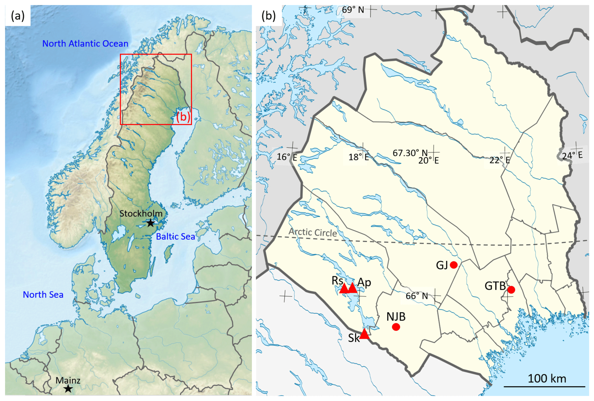
Figure 1Maps showing the sample sites in northern Sweden. (a) Topographic map of Scandinavia. (b) An enlargement of the red box in panel (a) showing Norrbotten County (yellow), a province in northern Sweden, and localities where bivalve shells (Margaritifera margaritifera) were collected and isotopes in rivers and precipitation were measured. The shell collection sites (filled circles) are coded as follows: NJB represents the Nuortejaurbäcken, GTB represents the Grundträsktjärnbäcken and GJ represents Görjeån River. Sk represents the Skellefte River (near Slagnäs), a GNIR site. The GNIP sites of Racksund and Arjeplog are represented by Rs and Ap, respectively. The base map in panel (a) is sourced from TUBS and used under a Creative Commons license: https://commons.wikimedia.org/wiki/File:Sweden_in_Europe_(relief).svg (last access: 5 February 2020). The base map in panel (b) is sourced from Erik Frohne (redrawn by Silverkey) and used under a Creative Commons license: https://commons.wikimedia.org/wiki/File:Sweden_Norrbotten_location_map.svg (last access: 5 February 2020).
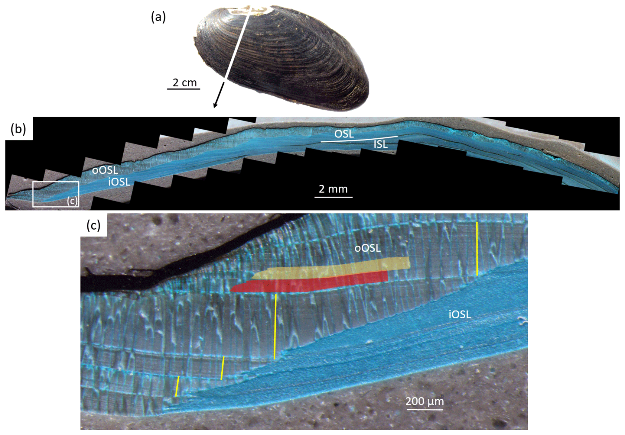
Figure 2Sclerochronological analysis of Margaritifera margaritifera. (a) The left valve of a freshwater pearl mussel. The cutting axis is indicated by a white line. Note the erosion in the umbonal shell portion. (b) A Mutvei-immersed shell slab showing the outer and inner shell layers (OSL and ISL, respectively) separated by the myostracum (white line). The OSL is further subdivided into an outer and inner portion (oOSL and iOSL, respectively). The ISL and iOSL consist of a nacreous microstructure, and the oOSL consists of a prismatic microstructure. (c) An enlargement of panel (b) shows the annual growth patterns. The annual increment width measurements (yellow) were completed as perpendiculars from the intersection of the oOSL and iOSL toward the next annual growth line. The semitransparent red and orange boxes schematically illustrate the micromilling sampling technique.
Table 1Shell of M. margaritifera from three streams in northern Sweden used in the present study for isotope and growth pattern analysis. The last hyphenated section of the specimen ID represents whether bivalves were collected alive (A) or dead (D), the specimen number and which valve was used (R denotes right and L denotes left).
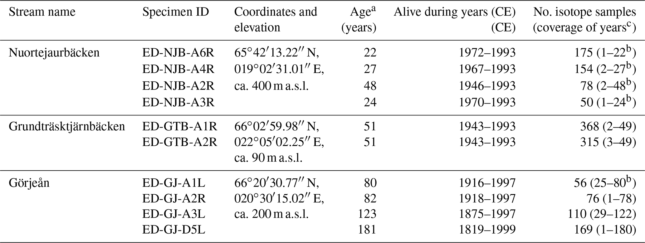
a Minimum estimate of life span. b Last sampled year incomplete. c Add 10 years to these values to obtain approximate ontogenetic years.
The bedrock in the catchments studied is dominated by orthogneiss and granodiorite. The vegetation at GTB (ca. 90 m a.s.l., above sea level) and GJ (ca. 200 m a.s.l.) consisted of a mixed birch forest, whereas conifers, shrubs and bushes dominated at NJB (ca. 400 m a.s.l.). Thus, the streams studied were rich in humin acids. The streams studied were fed by small upstream open (flow-through) lakes.
2.1 Sample preparation
The soft tissues were removed immediately after collection and shells were then air-dried. One valve of each specimen was wrapped in a protective layer of WIKO metal epoxy resin no. 5 and mounted to a Plexiglas cube using Gluetec Multipower plastic welder no. 3. Shells were then cut perpendicular to the growth lines using a low-speed saw (Buehler Isomet) equipped with a diamond-coated (low-diamond concentration) wafering thin blade (400 µm thickness). One specimen (ED-NJB-A3R) was cut along the longest axis, whereas all of the others were cut along the height axis from the umbo to the ventral margin (Fig. 2a). From each specimen, two ca. 3 mm thick shell slabs were obtained and mounted onto glass slides with the mirroring sides (the portions that were located to the left and right of the saw blade during the cutting process) facing upward. This method facilitated the temporal alignment of isotope data measured in one slab to growth patterns determined in the other shell slab. The shell slabs were ground on glass plates using suspensions of 800 and 1200 grit SiC powder and subsequently polished with Al2O3 powder (grain size of 1 µm) on a Buehler G-cloth. Between each grinding step and after polishing, the shell slabs were ultrasonically cleaned with water.
2.2 Shell growth pattern analysis
For growth pattern analysis, one polished shell slab was immersed in Mutvei's solution for 20 min at 37–40 ∘C under constant stirring (Schöne et al., 2005b). After careful rinsing in demineralized water, the stained sections were air-dried under a fume hood. Dyed thick-sections were then viewed under a binocular microscope (Olympus SZX16) that was equipped with sectoral dark-field illumination (Schott VisiLED MC1000) and were photographed using a Canon EOS 600D camera (Fig. 2b). The widths of the annual increments were determined to the nearest ca. 1 µm with image processing software (Panopea, © Peinl and Schöne). Measurements were completed in the outer portion of the outer shell layer (oOSL, consisting of prismatic microstructure) from the boundary between the oOSL and the inner portion of the outer shell layer (iOSL, consisting of nacrous microstructure) perpendicularly to the previous annual growth line (Fig. 2c). Annual increment width chronologies were detrended with stiff cubic spline functions and standardized to produce dimensionless measures of growth (standardized growth indices, i.e., SGI values – σ) following standard sclerochronological methods (Helama et al., 2006; Butler et al., 2013; Schöne, 2013). Briefly, for detrending, measured annual increment widths were divided by the data predicted by the cubic spline fit. From each resulting growth index, we subtracted the mean of all growth indices and divided the result by the standard deviation of all of the growth indices of the respective bivalve specimen. This transformation resulted in SGI chronologies. Due to low heteroscedasticity, no variance correction was needed (Frank et al., 2007). Uncertainties in annual increment measurements resulted in a SGI error of ±0.06σ.
2.3 Stable isotope analysis
The other polished shell slab of each specimen was used for stable isotope analysis. To avoid contamination of the shell aragonite powders (Schöne et al., 2017), the cured epoxy resin and the periostracum were completely removed prior to sampling. A total of 1551 powder samples (32–128 µg) were obtained from the oOSL by means of micromilling (Fig. 2c) under a stereomicroscope at 160× magnification. An equidistant sampling strategy was applied, i.e., the milling step size was held constant within each annual increment (Schöne et al., 2005c). We used a cylindrical, diamond-coated drill bit (1 mm diameter; Komet/Gebr. Brasseler GmbH and Co. KG, model no. 835 104 010) mounted on a Rexim Minimo drill. While the drilling device was affixed to the microscope, the sample was handheld during sampling. In early ontogenetic years, up to 16 samples were obtained between successive annual growth lines. In the latest ontogenetic portions of specimens ED-NJB-A2R (the last year of life) and ED-GJ-D6R (the last 9 years of life), each isotope sample represented 2–3 years.
Stable carbon and oxygen isotopes were measured at the Institute of Geosciences at the J.W. Goethe University of Frankfurt/Main (Germany). Carbonate powder samples were digested in He-flushed borosilicate Exetainer vials at 72 ∘C using a water-free phosphoric acid. The released CO2 gas was then measured in continuous-flow mode with a ThermoFisher MAT 253 gas source isotope ratio mass spectrometer coupled to a GasBench II. Stable isotope ratios were corrected against an NBS-19 calibrated Carrara marble ( ‰; ‰). Results are expressed as parts per thousand (‰) relative to the Vienna Pee Dee Belemnite (VPDB) scale. The long-term accuracy based on blindly measured reference materials with known isotope composition is better than 0.05 ‰ for both isotope systems. Note that no correction was applied for differences in fractionation factors of the reference material (calcite) and shells (aragonite; verified by Raman spectroscopy), because the paleothermometry equation used below (Eq. 2) also did not consider these differences (Füllenbach et al., 2015). However, the correction of −0.38 ‰ would be required if δ18O values of shells and other carbonates were compared with each other.
2.4 Instrumental data sets
Shell growth and isotope data were compared to a set of environmental variables including the station-based winter (DJFM) NAO index (obtained from https://climatedataguide.ucar.edu, last access: 9 April 2019) as well as oxygen isotope values of river water (δ18Ow) and weighted (corrected for precipitation amounts) oxygen isotope values of precipitation (δ18Op). Data on monthly river water and precipitation were sourced from the Global Network of Isotopes in Precipitation (GNIP) and the Global Network of Isotopes in Rivers (GNIR), available at the International Atomic Energy Agency:https://nucleus.iaea.org/wiser/index.aspx (last access: 1 April 2019). Furthermore, monthly air temperature (Ta) data came from the station Stensele, and are available at the Swedish Meteorological and Hydrological Institute: https://www.smhi.se (last access: 5 February 2020). From these data, the monthly stream water temperature (Tw) was computed using the summer air–stream water temperature conversion by Schöne et al. (2004a) and was supplemented by the standard errors of the slope and intercept:
2.5 Weighted annual shell isotope data
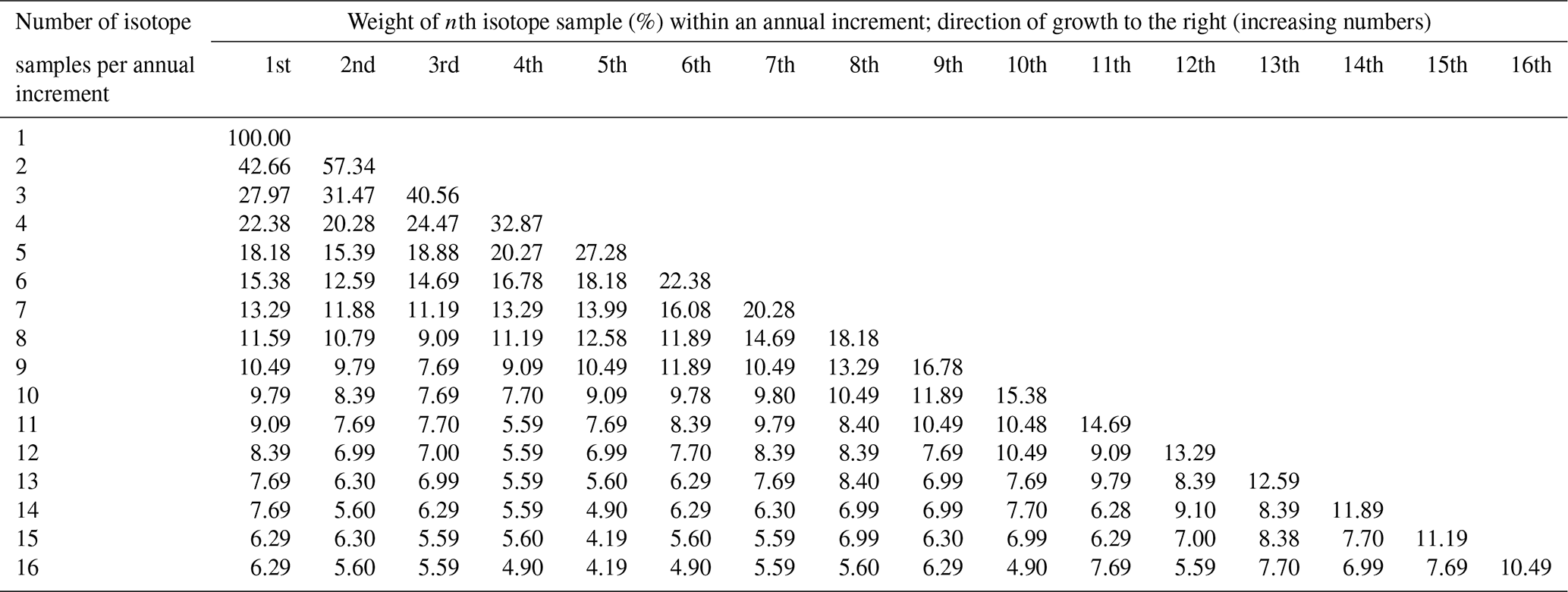
Because the shell growth rate varied during the growing season – with the fastest biomineralization rates occurring during June and July (Dunca et al., 2005) – the annual growth increments are biased toward summer, and powder samples taken from the shells at equidistant intervals represent different amounts of time. To compute growing season averages (henceforth referred to as “annual averages”) from such intra-annual shell isotope data (δ18Os, δ13Cs), weighted (henceforth denoted with an asterisk) annual means are thus needed, i.e., δ18O and δ13C values (Schöne et al., 2004a). The relative proportion of time of the growing season represented by each isotope sample was computed from a previously published intra-annual growth curve of juvenile M. margaritifera from Sweden (Dunca et al., 2005). For example, if four isotope samples were taken between two winter lines at equidistant intervals, the first sample would represent 22.38 % of the time of the main growing season duration, and the second, third and fourth would represent 20.28 %, 24.47 % and 32.87 % of the time of the main growing season, respectively (Table 2). Accordingly, the weighted annual mean isotope values (δ18O, δ13C) were calculated by multiplying these numbers (weights) by the respective δ18Os and δ13Cs values and dividing the sum of the products by 100 (see Supplement). The four isotope samples from the example above comprise the time intervals from 23 May to 22 June, 23 June to 21 July, 22 July to 25 August, and 26 August to 12 October, respectively. Missing isotope data due to lost powder, machine error, air in the Exetainer etc. were filled in using linear interpolation in 20 instances. We assumed that the timing and rate of seasonal growth remained nearly unchanged throughout the lifetime of the specimens and in the study region (see also Sect. 4).
Table 2Weights for isotope samples of Margaritifera margaritifera. Due to variations in the seasonal shell growth rate, each isotope sample taken at equidistant intervals represents different amounts of time. To calculate seasonal or annual averages from individual isotope data, the relative proportion of time of the growing season contained in each sample must be considered when weighted averages are computed. The duration of the growing season comprises 143 d and covers the time interval from 23 May to 12 October.
2.6 Reconstruction of oxygen isotope signatures of stream water on annual and intra-annual timescales
To assess how well the shells recorded δ18Ow values on inter-annual timescales, the stable oxygen isotope signature of stream water (δ18O) during the main growing season (“annual” δ18O) was reconstructed from δ18O data and the arithmetic average of (monthly) stream water temperatures, Tw, during the same time interval, i.e., 23 May–12 October. Using this approach, the effect of temperature-dependent oxygen isotope fractionation was removed from the δ18O data. For this purpose, the paleothermometry equation of Grossman and Ku (1986; corrected for the VPDB–VSMOW scale difference following Gonfiantini et al., 1995) was solved for δ18O, Eq. (2):
Because air temperature data were only available from 1860 onward, Tw values prior to that time were inferred from age-detrended and standardized annual growth increment data (SGI values) using a linear regression model similar to that introduced by Schöne et al. (2004a). In the revised model, SGI data of 25 shells from northern Sweden (15 published chronologies, provided in the article cited above, and 10 new chronologies from the specimens studied in the present paper) were arithmetically averaged for each year and then regressed against weighted annual water temperature, hereafter referred to as annual . The annual data consider variations in the seasonal shell growth rate. A total of 6.29 %, 25.49 %, 24.52 %, 21.92 %, 16.88 % and 4.90 % of the annual growth increment was formed in each month between May and October, respectively. The values were multiplied by Tw of the corresponding month and the sum of the products was divided by 100 to obtain the annual data. The revised (shell growth vs. temperature) model is as follows:
For coherency purposes, we also applied this model to post-1859 SGI values and computed stream water temperatures that were subsequently used to estimate δ18O values.
To assess how well the shells recorded δ18Ow values at intra-annual timescales, we focused on two shells from NJB (ED-NJB-A4R and ED-NJB-A6R), which provided the highest isotope resolution of 1–2 weeks per sample during the few years of overlap between the GNIP and GNIR data. Note that (only for this bivalve sampling locality) monthly instrumental oxygen isotope data were available from the GNIP and GNIR data sets (data by Burgman et al., 1981). The δ18Ow data were measured in the Skellefte River near Slagnäs, ca. 40 km SW of NJB (65∘34′59.50′′ N, 018∘10′39.12′′ E) and covered the time interval from 1973 to 1980. The δ18Op data came from Racksund (66∘02′60.00′′ N, 017∘37′60.00′′ E; ca. 75 km NW of NJB) and covered the time interval from 1975 to 1979. Because precipitation amounts were not available from Racksund, we computed average monthly precipitation amounts from data recorded at Arjeplog (66∘02′60.00′′ N, 017∘53′60.00′′ E) from 1961 to 1967 (see Supplement). Arjeplog is located ca. 65 km NW of NJB and ca. 12 km W of Racksund. Equation (2) was used to calculate δ18O values from individual δ18O data and water temperature that existed during the time when the respective shell portion was formed. Intra-annual water temperatures were computed as weighted averages, , from monthly Tw considering seasonal changes in the shell growth rate. For example, if four powder samples were taken from the shell at equidistant intervals within one annual increment, 6.29 % of the first sample was formed in May and 18.63 % was formed in June (sum ca. 25 %). The average temperature during that time interval is computed using these numbers as follows: (. A total of 6.86 % of the second sample from that annual increment formed in June and 17.97 % formed in July. Accordingly, the average temperature was (. Note that annual δ18O values can also be computed from intra-annual δ18O data, but this approach is much more time-consuming and complex than the method described further above. However, both methods produce nearly identical results (see Supplement).
2.7 Stable carbon isotopes of the shells
Besides the winter and summer NAO index, weighted annual stable carbon isotope data of the shells, δ13C values, were compared to shell growth data (SGI chronologies). Because the δ13C values could potentially be influenced by ontogenetic effects, the chronologies were detrended and standardized (δ13C) following methods typically used to remove ontogenetic age trends from annual increment width chronologies (see, e.g., Schöne, 2013). Detrending was carried out with cubic spline functions capable of removing any directed trend toward higher or lower values throughout the lifetime.
The lengths of the annual increment chronologies of M. margaritifera from the three streams studied (the Nuortejaurbäcken, Grundträsktjärnbäcken and Görjeån) ranged from 21 to 181 years and covered the time interval from 1819 to 1999 CE (Table 1). Because the umbonal shell portions were deeply corroded and the outer shell layer was missing – a typical feature of long-lived freshwater bivalves (Schöne et al., 2004a; Fig. 2a) – the actual ontogenetic ages of the specimens could not be determined and may have been up to 10 years higher than the ages listed in Table 1.
3.1 Shell growth and temperature
The 10 new SGI series from NJB, GTB and GJ were combined with 15 published annual increment series of M. margaritifera from the Pärlälven, Pärlskalsbäcken and Bölsmanån streams (Schöne et al., 2004a, b, 2005a) to form a revised Norrland master chronology. During the 50-year calibration interval from 1926 to 1975 (the same time interval was used in the previous study by Schöne et al., 2004a, b, 2005a), the chronology was significantly (p<0.05; note, all p values of linear regression analyses in this paper are Bonferroni-adjusted) and positively correlated (R=0.74; R2=0.55) with the weighted annual stream water temperature () during the main growing season (Fig. 3). These values were similar to the previously published coefficient of determination for a stacked record using M. margaritifera specimens from streams across Sweden (R2=0.60; Schöne et al., 2005a; note that this number is for SGI vs. an arithmetic annual Tw; a regression of SGI against weighted annual Tw returns an R2 of 0.64).
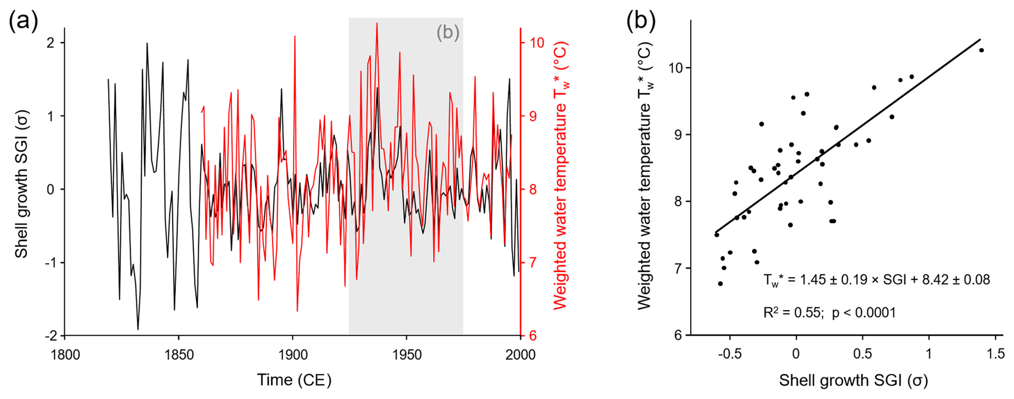
Figure 3(a) Time series and (b) cross-plot of the age-detrended and standardized annual shell growth rate (SGI values) and water temperature during the main growing season (23 May–12 October). Water temperatures were computed from monthly air temperature data using a published transfer function and considering seasonally varying rates of shell growth. The gray box in panel (a) denotes the 50-year calibration interval from which the temperature model (b) was constructed. As seen from the cross-plot in panel (b), 55 % of the variation in annual shell growth was highly significantly explained by water temperature. Higher temperature resulted in faster shell growth.
3.2 Shell stable oxygen isotope data
The shell oxygen isotope curves showed distinct seasonal and inter-annual variations (Figs. 4, 5). The former were particularly well developed in specimens from GTB and NJB (Fig. 4), which were sampled with a very high spatial resolution of ca. 30 µm (ED-GTB-A1R, ED-GTB-A2R, ED-NJB-A4R and ED-NJB-A6R). In these shells, up to 16 samples were obtained from single annual increments translating into a temporal resolution of 1–2 weeks per sample. Typically, the highest δ18Os values of each cycle occurred at the winter lines, and the lowest values occurred about half way between consecutive winter lines (Fig. 4). The largest seasonal δ18Os amplitudes of ca. 2.20 ‰ were measured in specimens from GTB (−8.68 ‰ to −10.91 ‰), and ca. 1.70 ‰ was measured in shells from NJB (−8.63 ‰ to −10.31 ‰).
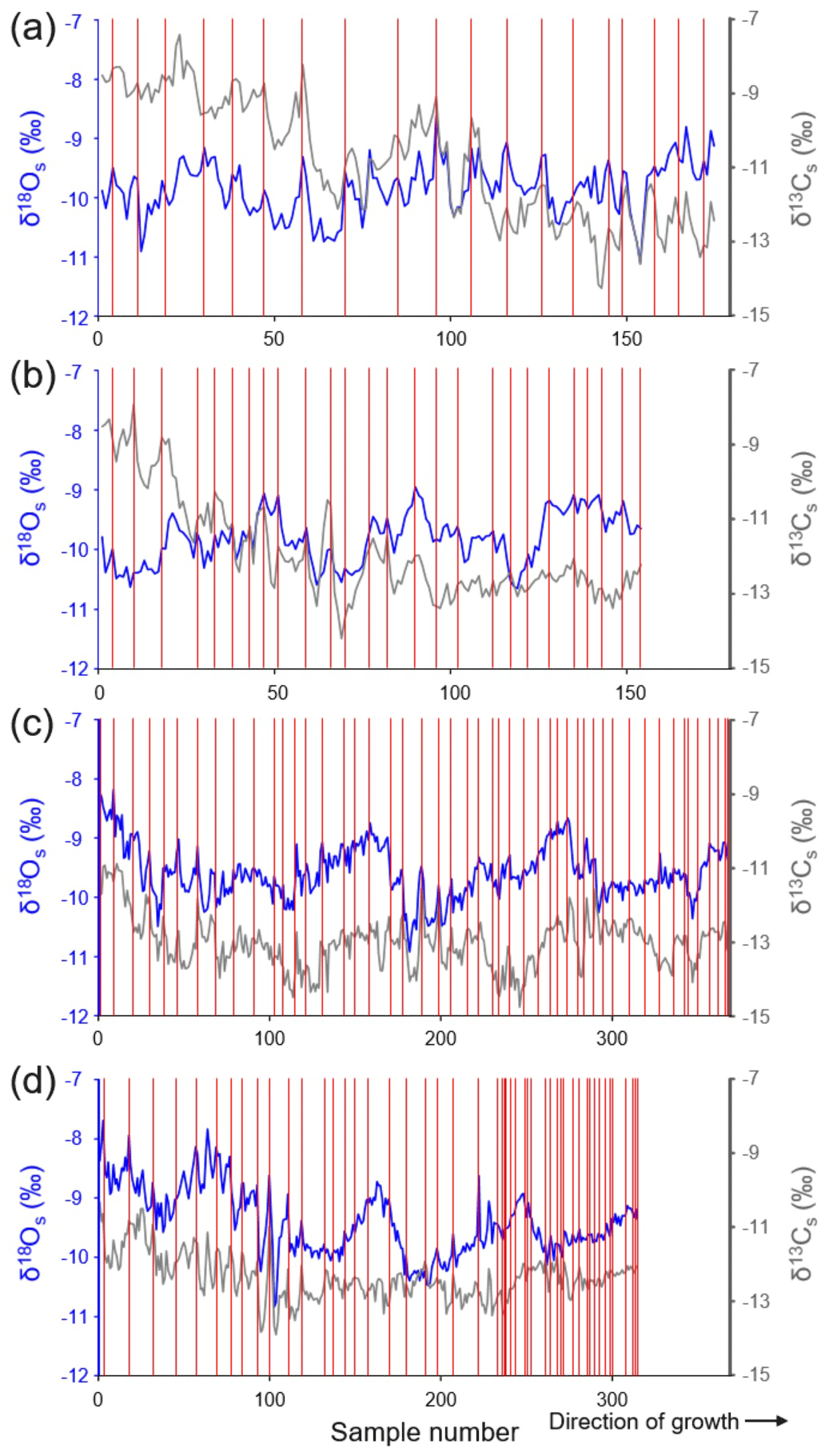
Figure 4Shell stable oxygen and carbon isotope chronologies from four specimens of Margaritifera margaritifera from Nuortejaurbäcken and Grundträsktjärnbäcken that were sampled with very high spatial resolution and from which the majority of the isotope data were obtained (Table 1): (a) ED-NJB-A6R, (b) ED-NJB-A4R, (c) ED-GTB-A1R and (d) ED-GTB-A2R. Individual isotope samples represent time intervals of a little as 6 d to 2 weeks in ontogenetically young shell portions and up to one full growing season in the last few years of life. Red vertical lines represent annual growth lines. Because the umbonal shell portions are corroded, the exact ontogenetic age at which the chronologies start cannot be provided. Assuming that the first 10 years of life are missing, sampling in panel (a) started in year 11, in panels (b) and (c) in year 12, and in panel (d) in year 13 (see also Table 1).
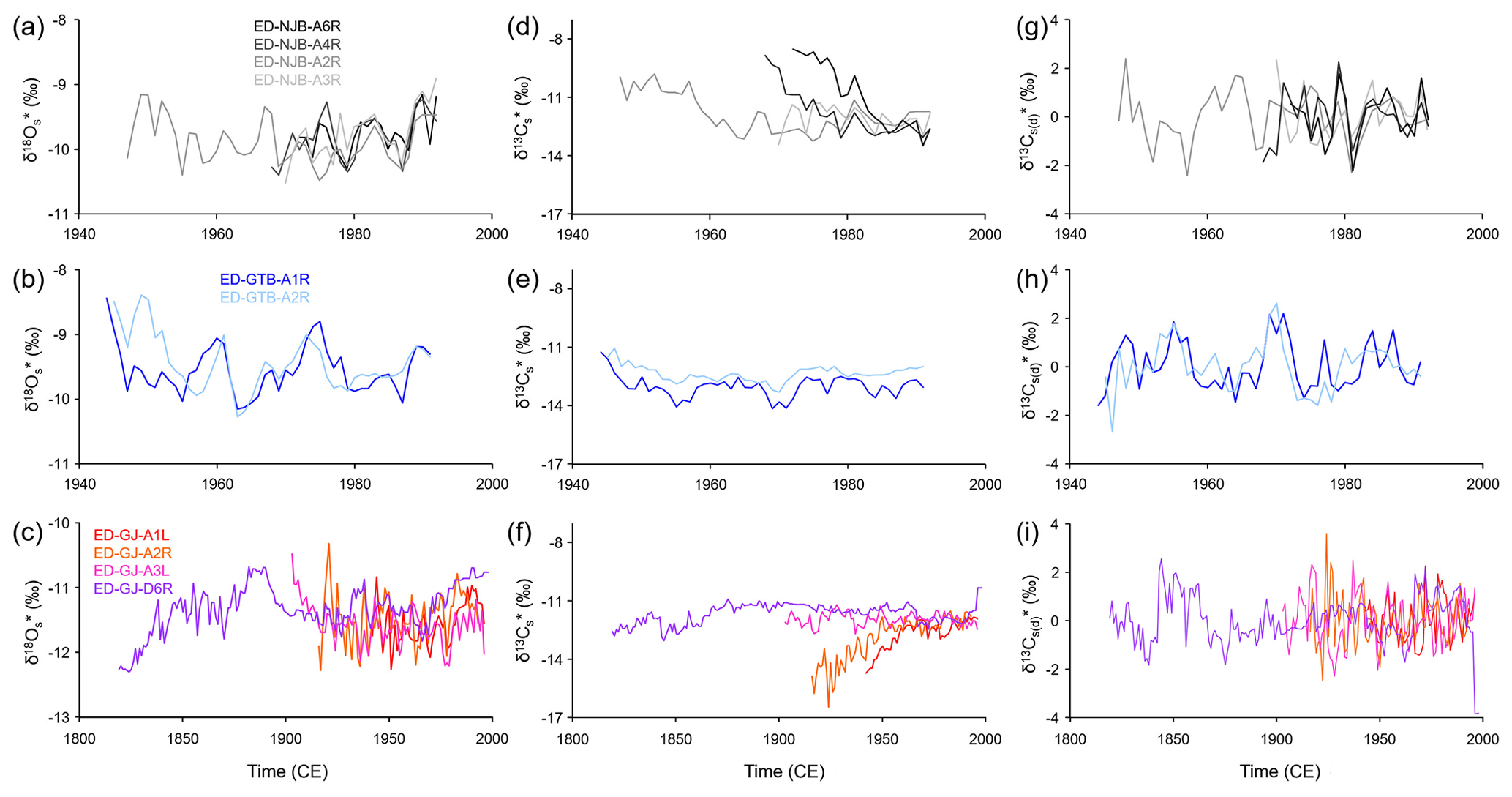
Figure 5Annual shell stable oxygen and carbon isotope chronologies of the specimens of Margaritifera margaritifera studied. Data were computed as weighted averages from intra-annual isotope data, i.e., growth rate-related variations were taken into consideration. Panels (a), (d) and (g) represent the stream Nuortejaurbäcken; panels (b), (e) and (h) represent the stream Grundträsktjärnbäcken; and panels (c), (f) and (i) represent Görjeån River. (a–c) Oxygen isotopes, (d–f) carbon isotopes, and (g–i) detrended and standardized carbon isotope values are also shown.
Weighted annual shell oxygen isotope (δ18O) values fluctuated on decadal timescales (common period of ca. 8 years) with amplitudes larger than those occurring on seasonal scales, i.e., ca. 2.50 ‰ and 3.00 ‰ in shells from NJB (−8.63 ‰ to −11.10 ‰) and GTB (−7.84 ‰ to −10.85 ‰), respectively (Fig. 5a, b). The chronologies from GJ also revealed a century-scale variation with minima in the 1820s and 1960s and maxima in the 1880s and 1990s (Fig. 5c). The δ18O curves of specimens from the same locality showed notable agreement in terms of absolute values and visual agreement (running similarity), specifically specimens from NJB and GTB (Fig. 5a, b). However, the longest chronology from GJ only showed slight agreement with the remaining three series from that site (Fig. 5c). The similarity among the series also changed through time (Fig. 5a, b ,c). In some years, the difference between the series was less than 0.20 ‰ at NJB (N=4) and GTB (N=2; 1983) and 0.10 ‰ at GJ (N=4; 1953), whereas, in other years, the differences varied by up to 0.82 ‰ at NJB and 1.00 ‰ at GTB and GJ. Average shell oxygen isotope chronologies of the three streams studied exhibited a strong running similarity (passed the “Gleichläufigkeitstest” by Baillie and Pilcher, 1973, for p<0.001) and were significantly positively correlated with each other (the R2 value of NJB vs. GTB was 0.34, NJB vs. GJ was 0.40 and GTB vs. GJ was 0.36 – all at p<0.0001).
3.3 Shell stable oxygen isotope data and instrumental records
At NJB – the only bivalve sampling site for which measured stream water isotope data were available from nearby localities – the May–October ranges of reconstructed and instrumental stream water δ18O values between 1973 and 1980 (excluding 1977 due to missing δ18Ow data) were in close agreement (shells were 2.83 and 3.19 ‰ vs. stream water which was 3.20 ‰; Fig. 6a). During the same time interval, arithmetic means ± 1 standard deviation of the shells were ‰ (ED-NJB-A6R; N=79) and ‰ (ED-NJB-A4R; N=44), whereas the stream water value was ‰ (Skellefte River; N=42). When computed from growing season averages (N=7), shell values were ‰ and ‰, respectively, and the stream water value was ‰. According to nonparametric t tests, these data sets are statistically indistinguishable. Furthermore, the inter-annual trends of δ18O and δ18Ow values were similar (Fig. 6a): values declined by ca. 1.00 ‰ between 1973 and 1977 followed by a slight increase of ca. 0.50 ‰ until 1980. In contrast to the damped stream water signal (the average seasonal range during the 4 years – 1975, 1976, 1978, and 1979 – for which both stream water and precipitation data were available was ‰), δ18Op values exhibited much stronger fluctuations at the seasonal scale (on average, ‰; extreme monthly values of −4.21 ‰ and −17.60 ‰; N=46; station Racksund; Fig. 6b) and on inter-annual timescales (unweighted annual averages of −11.41 ‰ to 13.68 ‰; weighted December–September averages of −9.54 ‰ to 13.16 ‰).
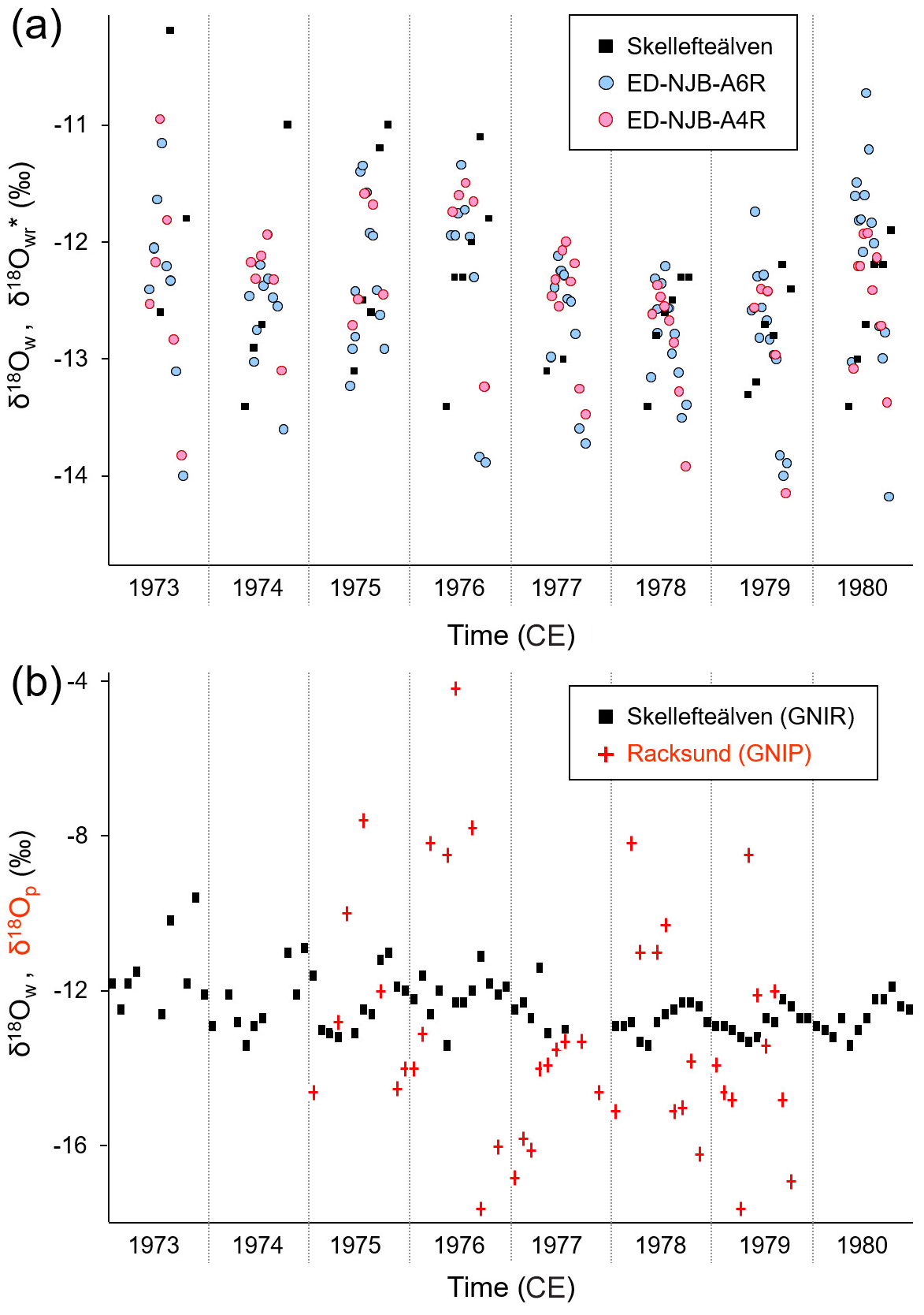
Figure 6Intra-annual stable oxygen isotope values (1973–1980). (a) Monthly isotopes measured in the Skellefte River (May–October) and weighted seasonal averages (δ18O) of two shells (Margaritifera margaritifera) from Nuortejaurbäcken (see Fig. 1). According to nonparametric t tests, instrumental and reconstructed oxygen isotope data are statistically indistinguishable. Also note that inter-annual changes are nearly identical. (b) Comparison of monthly oxygen isotope data in stream water (Skellefte River; May–October) and precipitation (Racksund; whole year).
Table 3Relationship between the stable oxygen isotope values in precipitation (amount-corrected δ18Op), river water and shells of Margaritifera margaritifera from Nuortejaurbäcken during different portions of the year (during the 4 years for which data from shells, water and precipitation were available: 1975, 1976, 1978, and 1979; hence N=4). The arithmetic mean δ18O values for each portion of the year are also given. The rationale behind the comparison of δ18O values of winter precipitation and spring (May–June) river water or shell carbonate is that the isotope signature of meltwater may have left a signal in the water. Statistically significant values (Bonferroni-adjusted p<0.05) are marked in bold. Isotope values next to months represent multiyear averages.
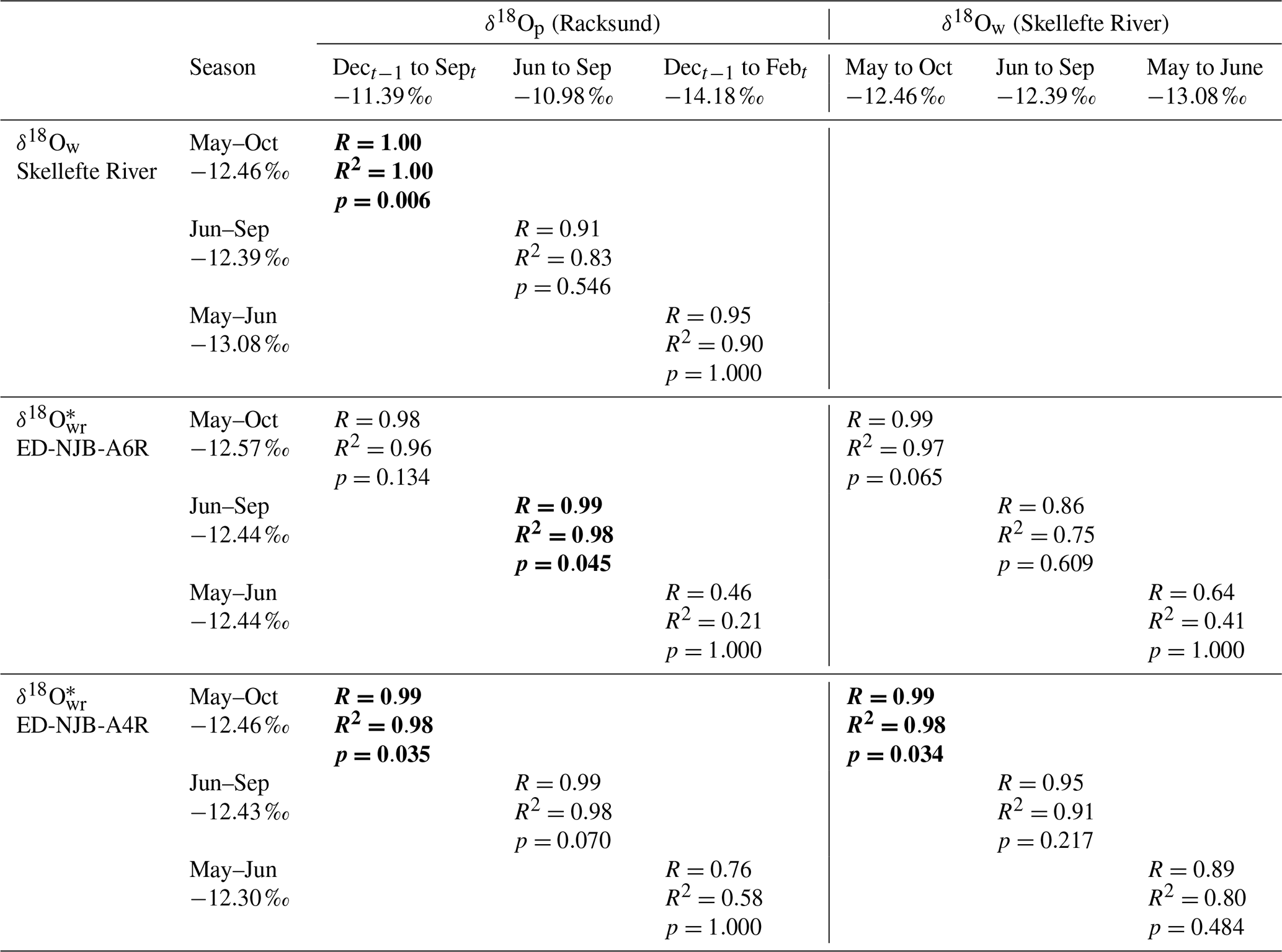
Despite the limited number of instrumental data, seasonally averaged δ18O data showed some – although not always statistically significant – agreement with δ18Ow and weighted δ18Op data (corrected for precipitation amounts), respectively, both in terms of correlation coefficients and absolute values (Table 3). These findings were corroborated by the regression analyses of instrumental δ18Op values against δ18Ow values (Table 3). For example, the oxygen isotope values of summer (June–September) precipitation were significantly (Bonferroni-adjusted p<0.05) and positively correlated with those of shell carbonate precipitated during the same time interval (98 % of the variability was explained in both specimens, but only at p<0.05 in ED-NJB-A6R). Likewise, δ18Ow and δ18Op values during summer were positively correlated with each other (R=0.91), although less significantly (p=0.546). Strong relationships were also found for δ18O and δ18Ow values during the main growing season as well as annual δ18O and December–September δ18Op values. The underlying assumption for the latter was that the δ18O average value reflects the combined δ18Op of snow precipitated during the last winter (received as meltwater during spring) and rain precipitated during summer. Instrumental data supported this hypothesis, because stream water δ18O values during the main growing season were highly significantly and positively correlated with December–September δ18Op data (Table 3). Conversely, changes in the isotope signal of winter (December–February) snow were only weakly and not significantly mirrored by changes in stream water oxygen isotope values during the snowmelt period (May–June) or in δ18O values from shell portions formed during the same time interval (Table 3). During the 4 years under study (1975, 1976, 1978 and 1979), measured and reconstructed δ18Ow values were nearly identical during the main growing season (δ18Ow of −12.46 ‰; δ18O of −12.57 ‰ and −12.46 ‰) and during summer (δ18Ow of −12.39 ‰; δ18O of −12.44 ‰ and −12.43 ‰) (Table 3). In contrast, isotopes in precipitation and river water showed larger discrepancies (see the text above, Fig. 6b and Table 3).
3.4 Shell stable oxygen isotope data and synoptic circulation patterns (NAO)
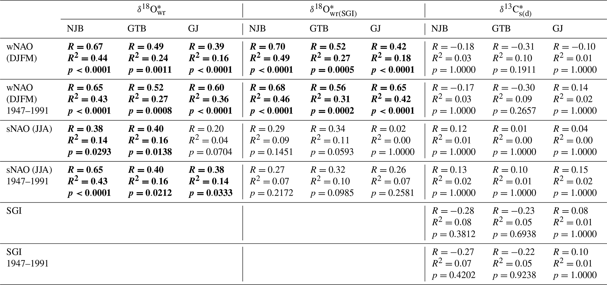
Site-specific annual δ18O (and δ18O) chronologies (computed as arithmetic averages of all chronologies at a given stream) were significantly (Bonferroni-adjusted p < 0.05) positively correlated with the NAO indices (Fig. 7, Table 4). In NAO+ years, the δ18O (and δ18O) values were higher than during NAO− years. The strongest correlation existed between the winter (December–March) NAO and δ18O (and δ18O) values at NJB (44 % to 49 % of the variability is explained). At GTB, the amount of variability explained ranged between 24 % and 27 %, whereas at GJ only 16 % to 18 % of the inter-annual δ18O (and δ18O) variability was explained by the winter NAO (wNAO) index. Between 1947 and 1991 (the time interval for which isotope data were available for all sites), the R2 values were more similar to each other and ranged between 0.27 and 0.46 (Table 4). All sites reflected well-known features of the instrumental NAO index series such as the recent (1970–2000) positive shift toward a more dominant wNAO, which delivered isotopically more positive (less depleted in 18O) winter precipitation to our region of interest (Fig. 7a, b, c). The correlation between δ18O (and δ18O) values and the summer (June–August) NAO index was much lower than for the wNAO, but likewise positive and sometimes significant at p<0.05 (Table 4). Between 1947 and 1991, 7 % to 43 % of the inter-annual oxygen isotope variability was explained by the summer NAO index.
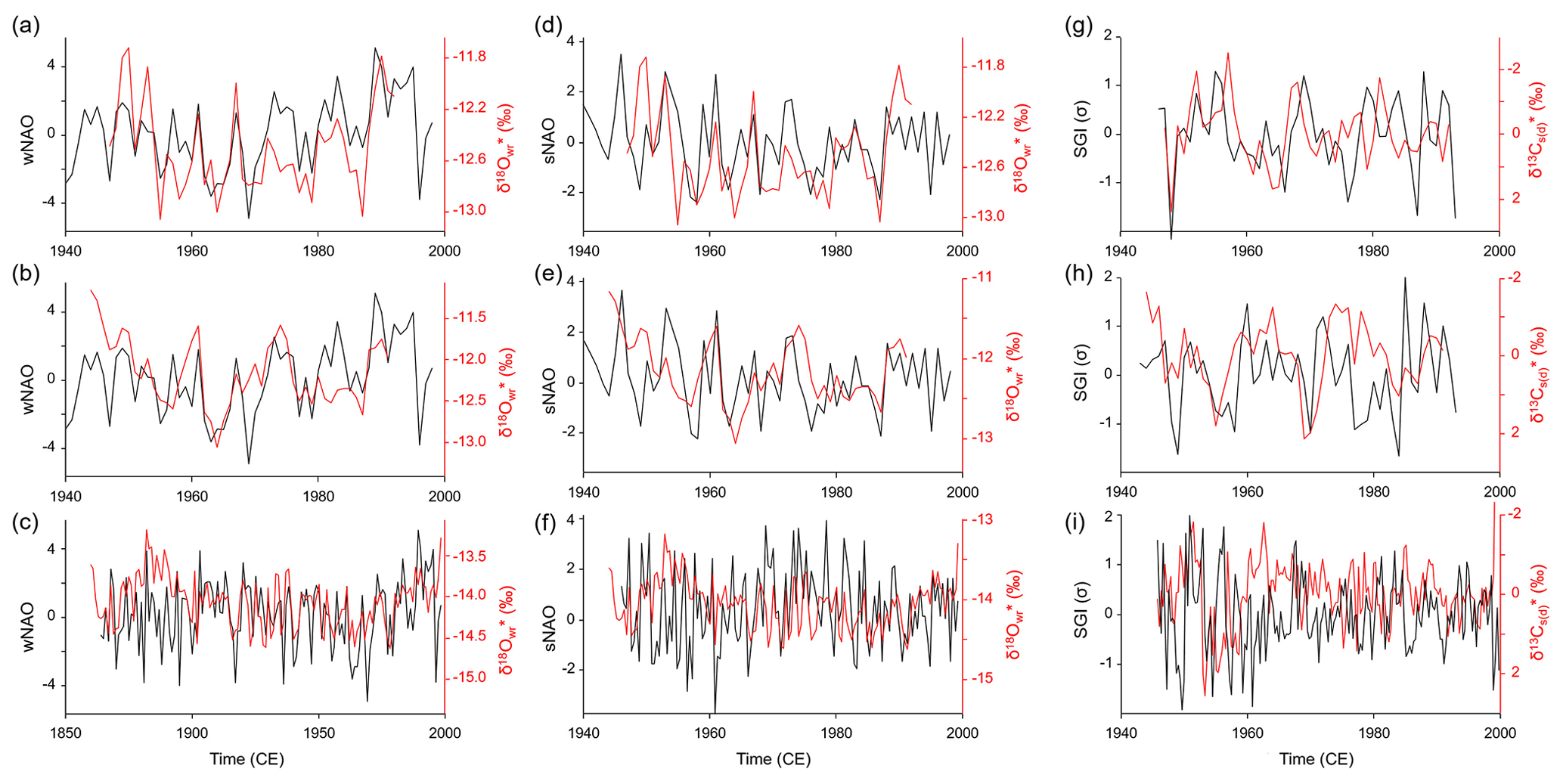
Figure 7Site-specific weighted annual δ18O (a–f) and δ13C (g–i) curves of Margaritifera margaritifera compared to the winter (a–c) and summer (d–f) North Atlantic Oscillation indices as well as the detrended and standardized shell growth rate (g–i). Panels (a), (d) and (g) show Nuortejaurbäcken, panels (b), (e) and (h) show Grundträsktjärnbäcken and panels (c), (f) and (i) show Görjeån.
Table 4Site-specific annual isotope chronologies of Margaritifera margaritifera shells linearly regressed against winter and summer NAO (wNAO and sNAO, respectively) as well as the detrended and standardized shell growth rate (SGI). δ18O data were computed from shell oxygen isotope data and temperature data were computed from instrumental air temperatures, whereas, in the case of δ18O data, temperatures were estimated from a growth-temperature model. See text for details. Statistically significant values (Bonferroni-adjusted p<0.05) are marked in bold.
We have also computed an average δ18O curve for the entire study region (Fig. 8a, b, c). Because the level (absolute values) of the three streams differed from each other (average δ18O values of NJB, GTB and GJ from 1947 to 1992 were −12.51 ‰, −12.21 ‰ and −14.16 ‰, respectively), the site-specific series were standardized and then arithmetically averaged. The resulting chronology, δ18O, was strongly positively and statistically significantly (Bonferroni-adjusted p value below 0.05) correlated with the wNAO index (56 % of the variability explained; Fig. 8a). Despite the limited instrumental data set, δ18O values of river water and precipitation were strongly positively correlated with the wNAO index (R2 values of 0.72 and 0.84, respectively; Fig. 8d, e), but the Bonferroni-adjusted p values exceeded 0.05 (note, the uncorrected p values were 0.07 and 0.03, respectively).
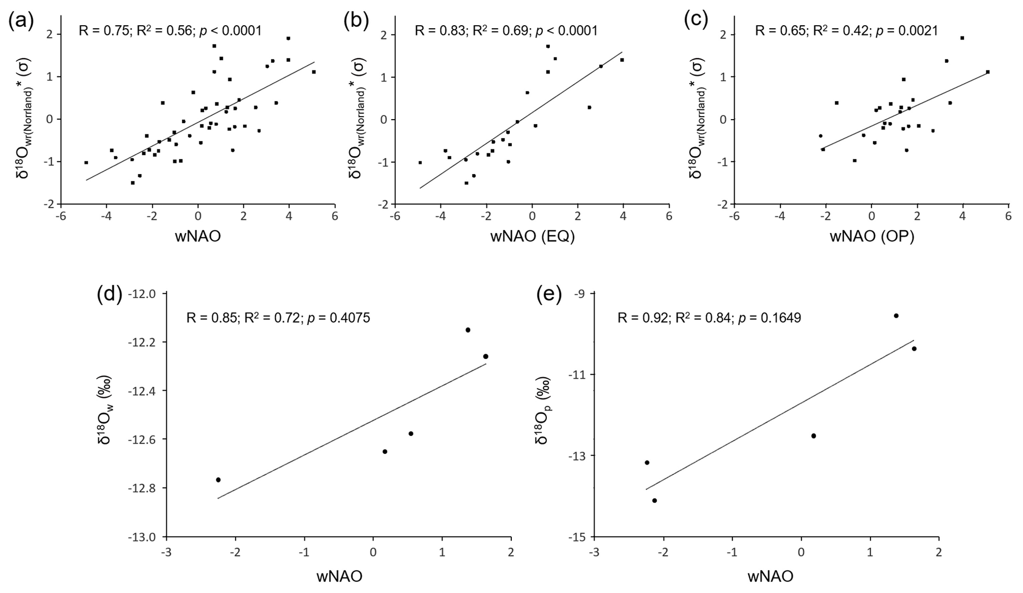
Figure 8Oxygen isotope data compared to the winter NAO index. (a) Standardized δ18O chronology of the study region compared to the winter NAO index between 1950 and 1998. (b) Same as in panel (a), but only when the East Atlantic Pattern (EA) index has the same sign (EQ) as the winter NAO. (c) Same as in panel (a), but only for cases when the EA index is in the opposite (OP) mode to the winter NAO. (d) δ18Ow values of the Skellefte River (during the growing season of the mussels – from May to October) in comparison with the winter NAO index (1975–1980). (e) δ18O values of precipitation (December–September) measured at Racksund in comparison with the winter NAO index (1975–1979).
3.5 Shell stable carbon isotope data
Shell stable carbon isotope (δ13Cs) data showed less distinct seasonal variations than δ18Os values, but the highest values were also often associated with the winter lines and the lowest values occurred between subsequent winter lines (Fig. 4). The largest seasonal amplitudes of ca. 3.90 ‰ were observed in specimens from NJB (−8.21 ‰ to −12.10 ‰) and ca. 1 ‰ smaller ranges at GTB (−10.97 ‰ to −13.88 ‰).
Weighted annual δ13C curves varied greatly from each other in terms of change throughout the lifetime of the organism, among localities and even at the same locality (Fig. 5d, e, f). Note that all curves started in early ontogeny (below the age of 10), except for ED-GJ-A1L and ED-GJ-A3L that began at a minimum age of 25 and 29, respectively (Table 1). Whereas two specimens from NJB (ED-NJB-A6R and ED-NJB-A4R) showed strong ontogenetic δ13C trends from ca. −8.70 ‰ to −12.50 ‰, weaker trends toward more negative values were observed in ED-NJB-A2R (ca. −10.00 ‰ to −11.70 ‰) and shells from GTB (ca. −11.50 ‰ to −13.00 ‰). Opposite ontogenetic trends occurred in ED-GJ-A1L and ED-GJ-A2R (ca. −15.00 ‰ to −12.00 ‰), but no trends at all were found in ED-NJB-A3R, ED-GJ-A3L and ED-GJ-D6R (fluctuations around −12.00 ‰). All curves were also overlain by some decadal variability (typical periods of 3–6, 13–16 and 60–80 years). Even after detrending and standardization (Fig. 5g, h, i), no statistically significant correlation at p<0.05 was found between the average δ13C curves of the three sites (NJB–GTB: , R2=0.01; NJB–GJ: , R2=0.03; GTB–GJ: R=0.10, R2=0.01). However, at each site, individual curves revealed reasonable visual agreement, specifically at NJB and GTB (Fig. 5g, h). At GJ, the agreement was largely limited to the low-frequency oscillations (Fig. 5i).
The detrended and standardized annual shell stable carbon isotope (δ13Cs(d)) curves showed no statistically significant (Bonferroni-adjusted p<0.05) agreement with the NAO indices or shell growth rate (SGI values) (Fig. 7, Table 4). A weak negative correlation (10 % explained variability) only existed between δ13C values and the wNAO at NJB. Some visual agreement was apparent between δ13Cs(d) values and SGI in the low-frequency realm. For example, at NJB, faster growth during the mid-1950s, 1970s, 1980s and 1990s fell together with lower δ13Cs(d) values (Fig. 7g). Likewise, at GTB, faster shell growth seemed to be inversely linked to δ13Cs(d) values (Fig. 7h).
4.1 Advantages and disadvantages of using bivalve shells for stream water δ18O reconstruction; comparison with sedimentary archives
Our results have shown that shells of freshwater pearl mussels from streams in northern Scandinavia (fed predominantly by small, open lakes and precipitation) can serve as a long-term, high-resolution archive of the stable oxygen isotope signature of the water in which they lived. Because δ18Ow values have a much lower seasonal amplitude than δ18Op values (i.e., δ18Ow signals are damped relative to δ18Op data as a result of the water transit times through the catchment of the stream), the observed and reconstructed stream water isotope signals mirror the seasonal and inter-annual variability in the δ18Op values. The NAO and subsequent atmospheric circulation patterns determine the origin of air masses and, subsequently, the δ18O signal in precipitation.
Compared with lake sediments, which have traditionally been used for similar reconstructions at nearby localities (e.g., Hammarlund et al., 2002; Andersson et al., 2010; Rosqvist et al., 2004, 2013), this new shell-based archive has a number of advantages.
The effect of temperature-dependent oxygen isotope fractionation can be removed from δ18Os values so that the stable oxygen isotope signature of the water in which the bivalves lived can be computed. This is possible by solving the paleothermometry equation of Grossman and Ku (1986) for δ18O (Eq. 2) and computing the oxygen isotope values of the water from those of the shells and stream water temperature. The stream water temperature during shell growth can be reconstructed from shell growth rate data (Eq. 3; Schöne et al., 2004a, b, 2005a) or the instrumental air temperature (Eq. 1; Morrill et al., 2005; Chen and Fang, 2015). However, similar studies in which the oxygen isotope composition of microfossils or authigenic carbonate obtained from lake sediments were used to infer the oxygen isotope value of the water merely relied on estimates of the temperature variability during the formation of the diatoms, ostracods and abiogenic carbonates among others, as well as how these temperature changes affected reconstructions of δ18Ow values (e.g., Rosqvist et al., 2013). In such studies, it was impossible to reconstruct the actual water temperatures from other proxy archives. Moreover, at least in some of these archives, such as diatoms, the effect of temperature on the fractionation of oxygen isotopes between the skeleton and the ambient water is still debated (Leng, 2006).
M. margaritifera precipitates its shell near oxygen isotope equilibrium with the ambient water, and shell δ18O values reflect stream water δ18O data. This may not be the case in all of the archives that have previously been used. For example, ostracods possibly exhibit vital effects (Leng and Marshall, 2004).
The shells can provide seasonally to inter-annually resolved data. In the present study, each sample typically represented as little as 1 week up to one full growing season (1 “year”; mid-May to mid-October; Dunca et al., 2005). In very slow growing shell portions of ontogenetically old specimens, individual samples occasionally covered 2 or, in exceptional cases, 3 years of growth which resulted in a reduction of variance. If required, a refined sampling strategy and computer-controlled micromilling could ensure that time-averaging consistently remains below 1 year. Such high-resolution isotope data can be used for a more detailed analysis of changes in the precipitation–runoff transformation across different seasons. Furthermore, the specific sampling method based on micromilling produced uninterrupted isotope chronologies, i.e., no shell portion of the outer shell layer remained un-sampled. Due to the high temporal resolution, bivalve shell-based isotope chronologies can provide insights into inter-annual- and decadal-scale paleoclimatic variability. With the new, precisely calendar-aligned data, it becomes possible to test hypotheses brought forward in previous studies according to which δ18O signatures of meteoric water are controlled by the winter and/or summer NAO (e.g., Rosqvist et al., 2007, 2013).
Each sample taken from the shells can be placed in a precise temporal context. The very season and exact calendar year during which the respective shell portion formed can be determined in shells of specimens with known dates of death based on the seasonal growth curve and annual increment counts. Existing studies suffer from the disadvantage that time cannot be precisely constrained, neither at seasonal nor annual timescales (unless varved sediments are available). However, isotope results can be biased toward a particular season of the year or a specific years within a decade. Such biases can be avoided with sub-annual data provided by bivalve shells.
In summary, bivalve shells can provide uninterrupted, seasonally to annually resolved, precisely temporally constrained records of past stream water isotope data that enable a direct comparison with climate indices and instrumental environmental data. In contrast to bivalve shells, sedimentary archives come with a much coarser temporal resolution. Each sample taken from sediments typically represents the average of several years, and the specific season and calendar year during which the ostracods, diatoms, authigenic carbonates etc. grew remains unknown. Conversely, the time intervals covered by sedimentary archives are much larger and can reveal century-scale and millennial-scale variations with much less effort than sclerochronology-based records. As such, the two types of archives could complement each other perfectly and increase the understanding of past climatic variability. For example, once the low-frequency variations have been reconstructed from sedimentary archives, a more detailed insight into seasonal to inter-annual climate variability can be obtained from bivalve shells. As long as the date of death of the bivalves is known, such records can be placed in absolute temporal context (calendar year). Although the same is currently impossible with fossil shells, each absolutely dated (radiocarbon and amino acid racemization dating) shell of a long-lived bivalve species can open a seasonally to annually resolved window into the climatic and hydrological past of a region of interest.
4.2 M. margaritifera shell δ18O values reflect stream water δ18O values
Unfortunately, complete, high-resolution and long-term records of δ18Ow values of the streams studied were not available. Such data are required for a direct comparison with those reconstructed from shells (δ18O or δ18O values) and to determine if the bivalves precipitated their shells near oxygen isotope equilibrium with the ambient water. However, one of the study sites (NJB) is located close to the Skellefte River, where δ18Ow values were irregularly analyzed between 1973 and 1980 (Fig. 6a) by the Water Resources Programme (GNIR data set). It should be noted that the δ18Ow data of GNIR merely reflect temporal snapshots, not actual monthly averages. In fact, the isotope signature of meteoric water can vary significantly on short timescales (e.g., Darling, 2004; Leng and Marshall, 2004; Rodgers et al., 2005). In addition, for some months, no GNIR data were available. In contrast, shell isotope data represent changes in the isotope composition of the water over coherent time intervals ranging from 1 week to 1 year (and in few cases 2 or 3 years). Due to the micromilling sampling technique, uninterrupted δ18Os time-series were available. Thus, it is compelling how well the ranges of intra-annual δ18O data compared to instrumental oxygen isotope data of the Skellefte River (Fig. 6a), and that summer averages as well as growing season averages of shells and GNIR were nearly identical (Table 3). Furthermore, in each stream studied, individual δ18O series agreed strongly with each other (Fig. 5). All of these aspects strongly suggest that shell formation occurred near equilibrium with the oxygen isotope composition of the ambient water, and M. margaritifera recorded changes in stream water δ18O values. Our conclusions are in agreement with previously published results from various different freshwater mussels (e.g., Dettman et al., 1999; Kaandorp et al., 2003; Versteegh et al., 2009) and numerous marine bivalves (e.g., Epstein et al., 1953; Mook and Vogel, 1968; Killingley and Berger, 1979).
4.3 Site-specific and synoptic information recorded in shell oxygen isotopes
Although individual chronologies from a given stream compared well to each other with respect to absolute values, the three sites studied differed by almost 2.00 ‰ (the average δ18O values between 1947 and 1992 were −12.51 ‰ at NJB, −12.21 ‰ at GTB and −14.16 ‰ at GJ; Figs. 5, 7). If our interpretation is correct and δ18Os values of the margaritiferids studied reflect the oxygen isotope signature of the water in which they lived, then these numbers reflect hydrological differences in the upstream catchment that are controlled by a complex set of physiographic characteristics: catchment size and elevation, transit times, upstream lake size and depth controlling the potential for evaporative depletion in 16O, stream flux rates, stream width and depth, humidity, wind speed, groundwater influx, differences in meltwater influx, an so on. (Peralta-Tapia et al., 2014; Geris et al., 2017; Pfister et al., 2017). However, detailed monitoring would be required to identify and quantify the actual reason(s) for the observed hydrological differences. Thus, we refrain from speculation.
Despite the site-specific differences described above, the δ18O chronologies of the three streams were significantly positively correlated with each other, suggesting that common environmental forcings controlled isotope changes throughout the study region. Previous studies suggest that these environmental forcings may include changes in the isotopic composition of precipitation, specifically the amount, origin and air mass trajectory of winter snow and summer rain, the timing of snowmelt as well as the condensation temperature (Rosqvist et al., 2013). The latter is probably the most difficult to assess, because no records are available documenting the temperature, height and latitude at which the respective clouds formed. Moreover, we cannot confidently assess the link between the isotope signature of precipitation and stream water because only limited and incoherent data sets are available from the study region. In addition, data on precipitation amounts were taken from another locality and another time interval. However, it is well known that precipitation in northern Scandinavia, particularly during winter, originates from two different sources, the Atlantic and arctic/polar regions (Rosqvist et al., 2013), and that the moisture in these air masses is isotopically distinct (Araguás-Araguás et al., 2000; Bowen and Wilkinson, 2002). During NAO+ years, the sea level pressure difference between the Azores High and the Iceland Low is particularly large resulting in mild, wet winters in central and northern Europe, with strong westerlies carrying heat and moisture across the Atlantic Ocean toward higher latitudes (Hurrell et al., 2003). During NAO− years, however, westerlies are weaker and the Polar Front is shifted southward, allowing arctic air masses to reach northern Scandinavia. Precipitation originating from the North Atlantic is isotopically heavier (δ18Op of −5.00 ‰ to −10.00 ‰) than precipitation from subarctic and polar regions (δ18Op of −10.00 ‰ to −15.00 ‰). Furthermore, changes in air mass properties over northern Europe are controlled by atmospheric pressure patterns in the North Atlantic, particularly the NAO during winter (Hurrell, 1995; Hurrell et al., 2003). The positive correlation between δ18O chronologies of the three streams studied and the wNAO index (Table 4, Figs. 7a, b, c, 8a) suggests that the shell isotopes recorded a winter precipitation signal, and this can be explained as follows. A larger proportion of arctic air masses carried to northern Scandinavia during winter resulted in lower δ18Op values, whereas the predominance of North Atlantic air masses caused the opposite. In NAO+ years, strong westerlies carried North Atlantic air masses far northward so that winter precipitation in northern Sweden had significantly higher δ18Op values than during NAO− years. When the NAO was in its negative state, precipitation predominantly originated from moisture from the polar regions which is depleted in 18O, and, hence, has lower δ18Op values. The specific isotope signatures in the streams were controlled by the snowmelt in spring. Essentially, the bivalves recorded the (damped) isotope signal of the last winter precipitation – occasionally mixed with spring and summer precipitation – in their shells. This hypothesis is supported by the correlation of the few available GNIP and GNIR data with the wNAO index (Fig. 8d, e). Rosqvist et al. (2007) hypothesized that the summer NAO strongly influences δ18Op values and, thus, the δ18Ow signature of the open, through-flow lakes in northern Scandinavia. However, our data did not support a profound influence of the summer NAO index on δ18O values (Fig. 7d, e, f). This conclusion is consistent with other studies suggesting that the summer NAO has a much weaker influence on European climate than the NAO during winter (e.g., Hurrell, 1995).
Following Baldini et al. (2008) and Comas-Bru et al. (2016), northern Sweden is not the ideal place to conduct oxygen-isotope-based wNAO reconstructions. Their models predicted only a weak negative correlation or no correlation between δ18Op values and the wNAO index in our study region (Baldini et al., 2008: Fig. 1; Comas-Bru et al., 2016: Fig. 3a). One possible explanation for this weak correlation is the limited and temporally incoherent GNIP data set in northern Sweden, from which these authors extracted the δ18Op data that were used to construct the numerical models. In contrast, δ18O data of diatoms from open lakes in northern Sweden revealed a strong link to the amount of precipitation and δ18Op values, which reportedly are both controlled by the predominant state of the NAO (Hammarlund et al., 2002; Andersson et al., 2010; Rosqvist et al., 2004, 2007, 2013). Findings of the present study substantiated these proxy-based interpretations. Furthermore, we presented, for the first time, oxygen isotope time-series with sufficient temporal resolution (annual) and the precise temporal control (calendar years) required for a year-to-year comparison with the NAO index time-series.
As Comas-Bru et al. (2016) further suggested, the relationship between δ18Op values and the wNAO index is subject to spatial nonstationarities, because the southern pole of the NAO migrates along a NE–SW axis in response to the state of another major atmospheric circulation mode in the North Atlantic realm known as the East Atlantic Oscillation or the East Atlantic Pattern (EA) (Moore and Renfrew, 2012; Moore et al., 2013; Comas-Bru and McDermott, 2014). Like the NAO, the EA is most distinct during winter and describes atmospheric pressure anomalies between the North Atlantic west of Ireland (low) and the subtropical North Atlantic (high). Through the interaction of these circulation patterns, the correlation between the wNAO and δ18Op values can weaken at times in certain regions. For example, when both indices are in their positive state, the jet stream shifts poleward (Woolings and Blackburn, 2012) and the storm trajectories that enter Europe in winter take a more northerly route (Comas-Bru et al., 2016). The δ18Op values will then be lower than during years. To identify whether this applies to the study region in question, we followed Comas-Bru et al. (2016) and tested if the relationship between the wNAO and reconstructed stream water oxygen isotope data remained significant during years when the signs of both indices were the same (EQ) and during years when they were opposite (OP). (Note that the EA index is only available from 1950 onward.) As demonstrated in Fig. 8b and c, the correlations between the region-wide shell-based oxygen isotope curve (δ18O) and the wNAO (EQ; R=0.83, R2=0.69, p<0.0001) as well as the wNAO (OP; R=0.65, R2=0.42, p=0.0021) remain positive and significant above the Bonferroni-adjusted 95 % confidence level. Hence, the relationship between the wNAO and δ18O values in the study region is not compromised by the EA; thus, δ18O values serve as a faithful proxy for the wNAO index.
4.4 Damped stream water oxygen isotope signals
Compared with the large isotope difference between winter precipitation sourced from SW or N air masses, the huge seasonal spread and inter-annual fluctuations of δ18Op values (seasonal fluctuation of −4.21 ‰ to −17.60 ‰, Fig. 6b; inter-annual, unweighted December–January averages of −10.18 ‰ to 14.64 ‰; weighted December–September averages of −9.54 ‰ to −14.10 ‰; Fig. 8e) as well as the predicted seasonal variance of δ18Ow values in the study region (Waterisotopes Database 2019: http://www.waterisotopes.org, last access: 25 May 2019: −8.70 ‰ to 17.30 ‰), the observed and shell-derived variance of the stream water δ18O values was notably small and barely exceeded 2.00 ‰, both on seasonal (Fig. 6) and inter-annual timescales (Fig. 5a, b, c). This figure agrees well with seasonal amplitudes determined in other streams at higher latitudes in the Northern Hemisphere (Halder et al., 2015) and can broadly be explained by catchment damping effects due to water collection, mixing, storage and release processes in upstream lakes, and groundwater from which these streams were fed. The catchment mean transit time (MTT), determined via a simple precipitation vs. stream flow isotope signal amplitude damping approach (as per de Walle et al., 1997), is approximately 6 months – corroborating the hypothesis of a mixed snowmelt and precipitation contribution to the stream water δ18O signal during the growing season.
The attenuated variance on inter-annual timescales can possibly be explained – amongst others – by inter-annual changes in the amount of winter precipitation and the timing of snowmelt. Colder spring temperatures typically resulted in a delayed snowmelt, so that lower oxygen isotope signatures still prevailed in the stream water when the main growing season of the bivalves started. However, winter precipitation amounts remained below average in NAO− years, meaning that the net effect on δ18Ow values in spring was less severe than the isotope shift in δ18Op values. In contrast, the amount of snow precipitated during NAO+ years was larger, but milder spring temperatures resulted in an earlier and faster snowmelt; thus, the effect on the isotope signature of stream water at the beginning of the growing season of the mussels likely remained moderate.
4.5 Sub-annual dating precision and relative changes in the seasonal shell growth rate
The precision with which the time that is represented by individual isotope samples can be determined depends on the validity of the seasonal growth model. We assumed that the timing of seasonal shell growth was similar to published data of M. margaritifera and remained the same in each year and each specimen. This may not be entirely correct, because the timing and rate of seasonal shell growth can potentially vary between localities, among years and among individuals; however, in M. margaritifera , the seasonal timing of shell growth is remarkably invariant across large distances (Dunca et al., 2005). A major dating error exceeding 4 weeks seems unlikely because the oxygen isotope series of individual specimens at each site were in good agreement. Presumably, the timing of seasonal shell growth is controlled by genetically determined biological clocks, which serve to maintain a consistent duration of the growing season (Schöne, 2008). Although shells grew faster in some years and slower in others, the relative seasonal changes in shell growth rates likely remained similar and consisted of a gradual increase as the water warmed and more food became available in spring and summer followed by a gradual decline as temperatures dropped in fall. It was further assumed that the timing of shell growth has not significantly changed through the lifetime of the specimens studied. In fact, if ontogenetic changes in seasonal growth traits had occurred, it would be impossible to crossdate growth curves from young and old individuals and construct master chronologies (Schöne et al., 2004a, b, 2005a; Helama et al., 2006; Black et al., 2010). Based on these arguments, seasonal dating errors were likely minor.
4.6 Shell stable carbon isotopes
Our results are consistent with previous studies using long-lived bivalves (Beirne et al., 2012; Schöne et al., 2005c, 2011), where δ13Cs chronologies of M. margaritifera did not show consistent ontogenetic trends but rather oscillated around an average value (ca. −12.00 ‰ to −13.00 ‰). The time series of NJB were too short to reject the hypothesis of directed trends throughout the lifetime of the organism; however, we propose here that the δ13Cs values of shells from that stream would also average out at ca. −12.50 ‰, as at the other two studied sites, if longer chronologies were available. If a contribution of metabolic CO2 to the shell carbonate exists in this species (which we cannot preclude because no δ13C values of the dissolved inorganic carbon, DIC, data are available for the streams studied), it likely remains nearly constant through the lifetime of the organism as it does in other long-lived bivalve mollusks (Schöne et al., 2005c, 2011; Butler et al., 2011; Reynolds et al., 2017). Observed stable carbon isotope signatures in the mussel shells are within the range of those expected and observed in stream waters of northern Europe (−10.00 ‰ to −15.00 ‰; Leng and Marshall, 2004).
Seasonal and inter-annual changes in δ13Cs values could be indicative of changes in primary production, food composition, respiration and the influx of terrestrial detritus. However, in the absence of information on how the environment of the streams that were studied changed through time, we can only speculate about possible causes of temporal δ13CDIC variations. For example, increased primary production in the water would not only have propelled shell growth rate but would also have resulted in a depletion of 12C in the DIC pool and, thus, higher δ13CDIC and δ13Cs values. However, just the opposite was observed on seasonal and inter-annual timescales. The highest δ13Cs values often occurred near the annual growth lines, i.e., during times of slow growth, and, although not statistically significant, annual δ13C values at NJB and GTB were inversely related to the shell growth rate (Fig. 7g, h, Table 4). Accordingly, δ13C values do not seem to reflect phytoplankton dynamics. Another possibility is that a change in the composition of mussel food occurred which changed the shell stable carbon isotope values without a statistically significant effect on shell growth rate. Because the isotope signatures of potential food sources differ from each other (e.g., Gladyshev, 2009), a change in the relative proportions of phytoplankton, decomposing plant litter from the surrounding catchment vegetation, bacteria, particulate organic matter derived from higher organisms etc. could have left a footprint in the δ13C values. Furthermore, seasonal and inter-annual changes in respiration or the influx of terrestrial detritus may have changed the isotope signature of the DIC pool and, thus, the shells. Support for the latter comes from the weak negative correlation between δ13C values and the wNAO (Table 4; without Bonferroni correction, p values remained below 0.05). After wet (snow-rich) winters (NAO+ years), stronger terrestrial runoff may have flushed increased amounts of light carbon into the streams which lowered δ13CDIC values. To test these hypotheses, data on the stable carbon isotope signature of digested food and DIC would be required, which is a task for subsequent studies.
4.7 Error analysis and sensitivity tests
To test the robustness of the findings presented in Tables 3 and 4 as well as their interpretation, we have propagated all uncertainties associated with measurements and modeled data and randomly generated δ18O, δ18O, δ18O and δ13C chronologies (via Monte Carlo simulation). A brief overview of the errors and simulation procedures are provided below.
Table 5Results of sensitivity tests. To test the robustness of statistically significant correlations presented in Tables 3 and 4, uncertainties (one of them the error associated with the reconstruction of stream water temperatures, Tw, from air temperatures, Ta) were propagated and used to randomly generate δ18O chronologies, which were subsequently regressed against the winter North Atlantic Oscillation (wNAO) indices. Simulations were computed with propagated values of 2.07 and 0.90 ∘C. See text for details. Statistically significant values (Bonferroni-adjusted p<0.05) are marked in bold.
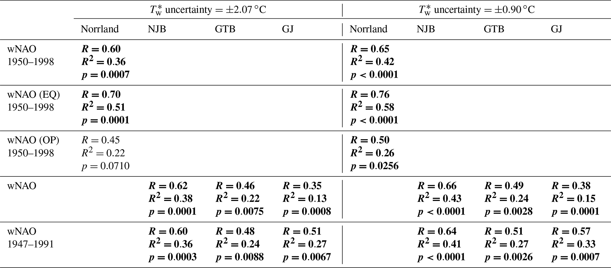
Water temperature estimates (Eq. 1) were associated with an error (1 standard deviation) of ±2.07 ∘C. Amongst others, this large uncertainty results from the combination of temperature data of four different streams, which all varied with respect to the average temperature and year-to-year variability. The error exceeds the inter-annual variance (1 standard deviation of ±0.90 ∘C) of the instrumental water temperature average (8.64 ∘C) by more than 2 times. Instead of reconstructing Tw from Ta with an uncertainty of ±2.07 ∘C, we could have assumed a constant water temperature value of 8.64 ∘C with an uncertainty of only ±0.90 ∘C. However, our goal was to improve the δ18O reconstructions by taking the actual year-to-year temperature variability into account. To simulate the effect of different temperature uncertainties, we randomly generated 1000 chronologies with an error of ±0.90 ∘C as well as 1000 chronologies with an error of ±2.07 ∘C. Both sets of simulated time-series were used in subsequent calculations. Errors involved with shell growth patterns include the measurement error (±1 µm equivalent to an SGI error of ±0.06 units) and the variance of crossdated SGI data. In different calendar years, the standard error of the mean of the 25 SGI chronologies ranged between ±0.03 and ±0.66 SGI units. The measurement and crossdating uncertainties were propagated, and 1000 new SGI chronologies were randomly generated and regressed against simulated chronologies. The uncertainty of the new SGI vs. model (standard error of ±1.35 ∘C) was propagated in subsequent calculations of δ18O values using Eq. (2). A third set of uncertainties was associated with isotope measurements (analytical precision error, 1 standard deviation ‰), the calculation of site-specific annual averages from contemporaneous specimens (±0.11 ‰ to ±0.15 ‰ for δ18O on average; ±0.37 ‰ to ±0.42 ‰ for δ13C on average) and the calculation of the Norrland average. All errors were propagated and new δ18O, δ18O, δ18O and δ13C chronologies were simulated (1000 representations each). The chronologies simulated were regressed against NAO and SGI chronologies (results of sensitivity tests for the regressions of δ18O and δ18O values vs. wNAO indices are given in Table 5).
According to the complex simulation experiments, the observed links between reconstructed stream water oxygen isotope values and the wNAO largely remained statistically robust irrespective of which error was assumed (Table 5). This outcome is not particularly surprising given that even the annual δ18Os chronologies of the studies' specimens were strongly coherent, and values fluctuated at timescales similar to that of the wNAO (Fig. 4). Apparently, decadal-scale atmospheric circulation patterns indeed exert a strong control over the isotope signature of stream water in the study area. However, none of the correlations between shell isotope data and the sNAO were statistically significant at the predefined value of p≤0.05. The importance of summer rainfall seems much less important for the isotope value of stream water than winter snow. As before, the relationship between stable carbon isotope data of the shells and climate indices as well as the shell growth rate remained weak and were statistically not significant. Inevitably, the propagated errors, specifically the uncertainty associated with the reconstruction of the stream water temperature from air temperature resulted in a notable drop in the amount of variability explained and in the statistical probability (Table 5). The use of instrumental water temperatures could greatly improve the reconstruction of δ18O values, as the measurement error would be of the order of 0.1 ∘C instead of 2.07 or 0.90 ∘C. Thus, future calibration studies should be conducted in monitored streams.
Stable oxygen isotope values in shells of freshwater pearl mussels, M. margaritifera, from streams in northern Sweden mirror stream water stable oxygen isotope values. Despite a well-known damping of the precipitation signal in stream water isotope records, these mollusks archive local precipitation and synoptic atmospheric circulation signals, specifically the NAO during winter. Stable carbon isotope data of the shells are more challenging to interpret, but they seem to record local environmental conditions such as changes in DIC and/or food composition. Future studies should be conducted in streams in which temperature, DIC and food levels are closely monitored to further improve the reconstruction of stream water δ18O values from δ18Os data and better understand the meaning of δ13Cs fluctuations.
The bivalve shell oxygen isotope record presented here extends back to 1819 CE, but there is the potential to develop longer isotope chronologies via the use of fossil shells of M. margaritifera collected in the field or taken from museum collections. With suitable material and by applying the crossdating technique, the existing chronology could probably be extended by several centuries back in time. Stream water isotope records may shed new light on pressing questions related to climate change impacts on river systems, the mechanistic understanding of water flow and quality controlling processes, calibration and validation of flow and transport models, climate and Earth system modeling, time variant catchment travel time modeling, and so on. Longer and coherent chronologies are essential to reliably identify multidecadal-scale and century-scale climate dynamics. Even individual radiocarbon-dated fossil shells that do not overlap with the existing master chronology can provide valuable paleoclimate information, because each M. margaritifera specimen can open a seasonally to annually resolved, multiyear window into the history of streams.
All data and code used in this study are available from the authors upon request. Additional supplementary files are available at https://www.paleontology.uni-mainz.de/datasets/HESS_2019_337_supplements.zip (last access: 5 February 2020).
Bivalve shell samples are archived and stored in the paleontological collection of the University of Mainz.
The supplement related to this article is available online at: https://doi.org/10.5194/hess-24-673-2020-supplement.
BRS designed the study, performed the analyses and wrote the paper; AEM and SMB conducted the field work and collected samples; SMB sampled the shells and temporally aligned the isotope data; JF isotopically analyzed the shell powder; LP conducted MTT calculations. All authors jointly contributed to the discussion and interpretation of the data.
The authors declare that they have no conflict of interest.
We thank Denis Scholz and Erika Pietroniro for constructive discussions. We are grateful for comments and suggestions provided by two anonymous reviewers that greatly improved the quality of this article. This study has been made possible through a research grant by the Deutsche Forschungsgemeinschaft (DFG) to BRS (grant no. SCHO793/1).
This research has been supported by the Deutsche Forschungsgemeinschaft (grant no. SCHO793/1).
This open-access publication was funded
by Johannes Gutenberg University Mainz.
This paper was edited by Brian Berkowitz and reviewed by two anonymous referees.
Andersson, S., Rosqvist, G., Leng, M. J., Wastegard, S., and Blaauw, M.: Late Holocene climate change in central Sweden inferred from lacustrine stable isotope data, J. Quaternary Sci., 25, 1305–1316, https://doi.org/10.1002/jqs.1415, 2010.
Araguás-Araguás, L., Froehlich, K., and Rozanski, K.: Deuterium and oxygen-18 isotope composition of precipitation and atmospheric moisture, Hydrol. Process., 14, 1341–1355, https://doi.org/10.1002/1099-1085(20000615)14:8<1341::AID-HYP983>3.0.CO;2-Z, 2000.
Baillie, M. G. L. and Pilcher, J. R.: A simple crossdating program for tree-ring research, Tree-ring Bull., 33, 7–14, 1973.
Baldini, L. M., McDermott, F., Foley, A. M., and Baldini, J. U. L.: Spatial variability in the European winter precipitation δ18O-NAO relationship: Implications for reconstructing NAO-mode climate variability in the Holocene, Geophys. Res. Lett., 35, L04709, https://doi.org/10.1029/2007GL032027, 2008.
Beirne, E. C., Wanamaker Jr., A. D., and Feindel, S. C.: Experimental validation of environmental controls on the δ13C of Arctica islandica (ocean quahog) shell carbonate, Geochim. Cosmochim. Ac., 84, 395–409, https://doi.org/10.1016/j.gca.2012.01.021, 2012.
Black, B. A., Dunham, J. B., Blundon, B. W., Raggon, M. F., and Zima, D.: Spatial variability in growth-increment chronologies of long-lived freshwater mussels: Implications for climate impacts and reconstructions, Écosci., 17, 240–250, https://doi.org/10.2980/17-3-3353, 2010.
Bowen, G. J. and Wilkinson, B.: Spatial distribution of δ18O in meteoric precipitation, Geology, 30, 315–318, https://doi.org/10.1130/0091-7613(2002)030<0315:SDOOIM>2.0.CO;2, 2002.
Burgman, J. O., Eriksson, E., and Westman, F.: Oxygen-18 variation in river waters in Sweden. Avd. Hydrol. Unpublished Report, Uppsala Univ., Naturgeogr. Inst., Uppsala, Sweden, 42 p., 1981.
Butler, P. G., Wanamaker Jr., A. D., Scourse, J. D., Richardson, C. A., and Reynolds, D. J.: Long-term stability of δ13C with respect to biological age in the aragonite shell of mature specimens of the bivalve mollusk Arctica islandica, Palaeogeogr. Palaeocl., 302, 21–30, https://doi.org/10.1016/j.palaeo.2010.03.038, 2011.
Butler, P. G., Wanamaker Jr., A. D., Scourse, J. D., Richardson, C. A., and Reynolds, D. J.: Variability of marine climate on the North Icelandic Shelf in a 1357-year proxy archive based on growth increments in the bivalve Arctica islandica, Palaeogeogr. Palaeocl., 373, 141–151, https://doi.org/10.1016/j.palaeo.2012.01.016, 2013.
Chen, G. and Fang, X.: Accuracy of hourly water temperatures in rivers calculated from air temperatures, Water 7, 1068–1087, https://doi.org/10.3390/w7031068, 2015.
Comas-Bru, L. and McDermott, F.: Impacts of the EA and SCA patterns on the European twentieth century NAOwinter climate relationship, Q. J. Roy. Meteor. Soc., 140, 354–363, https://doi.org/10.1002/qj.2158, 2014.
Comas-Bru, L., McDermott, F., and Werner, M.: The effect of the East Atlantic pattern on the precipitation δ18O-NAO relationship in Europe, J. Clim. Dyn., 47, 2059–2069, https://doi.org/10.1007/s00382-015-2950-1, 2016.
Darling, W. G.: Hydrological factors in the interpretation of stable isotopic proxy data present and past: a European perspective, Quaternary Sci. Rev., 23, 743–770, https://doi.org/10.1016/j.quascirev.2003.06.016, 2004.
Darling, W. G. and Bowes, M. J.: A long-term study of stable isotopes as tracers of processes governing water flow and quality in a lowland river basin, Hydrol. Process., 30, 2178–2195, https://doi.org/10.1016/j.quascirev.2003.06.016, 2016.
Dettman, D. L, Reische, A. K., and Lohmann, K. C.: Controls on the stable isotope composition of seasonal growth bands in aragonitic fresh-water bivalves (unionidae), Geochim. Cosmochim. Ac., 63, 1049–1057, https://doi.org/10.1016/S0016-7037(99)00020-4, 1999.
DeWalle, D. R., Edwards, P. J., Swistock, B. R., Aravena, R., and Drimmie, R. J.: Seasonal isotope hydrology of three Appalachian forest catchments, Hydrol. Process., 11, 1895–1906, 1997.
Dunca, E. and Mutvei, H.: Comparison of microgrowth pattern in Margaritifera margaritifera shells from south and north Sweden, Am. Malacol. Bull., 16, 239–250, 2001.
Dunca, E., Schöne, B. R., and Mutvei, H.: Freshwater bivalves tell of past climates: But how clearly do shells from polluted rivers speak? Palaeogeogr. Palaeocl., 228, 43–57, https://doi.org/10.1016/j.palaeo.2005.03.050, 2005.
Epstein, S., Buchsbaum, R., Lowenstam, H. A., and Urey, H. C.: Revised carbonate-water isotopic temperature scale, Geol. Soc. Am. Bull., 64, 1315–1326, https://doi.org/10.1130/0016-7606(1953)64[1315:RCITS]2.0.CO;2, 1953.
Frank, D., Esper, J., and Cook, E. R.: Adjustment for proxy number and coherence in a large-scale temperature reconstruction, Geophys. Res. Lett., 34, L16709, https://doi.org/10.1029/2007GL030571, 2007.
Füllenbach, C. S., Schöne, B. R., and Mertz-Kraus, R.: Strontium/lithium ratio in shells of Cerastoderma edule (Bivalvia) – A new potential temperature proxy for brackish environments, Chem. Geol., 417, 341–355, https://doi.org/10.1016/j.chemgeo.2015.10.030, 2015.
Geeza, T. J., Gillikin, D. P., Goodwin, D. H., Evans, S. D., Watters, T., and Warner, N. R.: Controls on magnesium, manganese, strontium, and barium concentrations recorded in freshwater mussel shells from Ohio, Chem. Geol., 526, 142–152, https://doi.org/10.1016/j.chemgeo.2018.01.001, 2019.
Geeza, T. J., Gillikin, D. P., McDevitt, B., Van Sice, K., and Warner, N. R.: Accumulation of Marcellus Formation oil and gas wastewater metals in freshwater mussel shells, Environ. Sci. Technol., 52, 10883–10892, https://doi.org/10.1021/acs.est.8b02727, 2020.
Geist, J., Auerswald, K., and Boom, A.: Stable carbon isotopes in freshwater mussel shells: Environmental record or marker for metabolic activity?, Geochim. Cosmochim. Ac. 69, 3545–3554, https://doi.org/10.1016/j.gca.2005.03.010, 2005.
Geris, J., Tetzlaff, D., McDonnell, J. J., and Soulsby, C., Spatial and temporal patterns of soil water storage and vegetation water use in humid northern catchments, Sci. Total Environ. 595, 486–493, https://doi.org/10.1016/j.scitotenv.2017.03.275, 2017.
Gladyshev, M. I.: Stable isotope analyses in aquatic ecology (a review), Journal of Siberian Federal University – Biology, 4, 381–402, https://doi.org/10.17516/1997-1389-0220, 2009.
Gonfiantini, R., Stichler, W., and Rozanski, K.: Standards and intercomparison materials distributed by the International Atomic Energy Agency for stable isotope measurements (IAEA-TECDOC-825), International Atomic Energy Agency (IAEA), Vienna, Austria, 13–29, available at: https://www-pub.iaea.org/MTCD/publications/PDF/te_825_prn.pdf (last access: 5 February 2020), 1995.
Grossman, E. L. and Ku, T.-L.: Oxygen and carbon isotope fractionation in biogenic aragonite; temperature effects, Chem. Geol. Isot. Geosci. Sect., 59, 59–74, https://doi.org/10.1016/0168-9622(86)90057-6, 1986.
Halder, J., Terzer, S., Wassenaar, L. I., Araguás-Araguás, L. J., and Aggarwal, P. K.: The Global Network of Isotopes in Rivers (GNIR): integration of water isotopes in watershed observation and riverine research, Hydrol. Earth Syst. Sci., 19, 3419–3431, https://doi.org/10.5194/hess-19-3419-2015, 2015.
Hammarlund, D., Barnekow, L., Birks, H. J. B., Buckardt, B., and Edwards, T. W. D.: Holocene changes in atmospheric circulation recorded in the oxygen-isotope stratigraphy of lacustrine carbonates from northern Sweden, Holocene, 12, 339–351, https://doi.org/10.1191/0959683602hl548rp, 2002.
Helama, S., Schöne, B. R., Black, B. A., and Dunca, E.: Constructing long-term proxy series for aquatic environments with absolute dating control using a sclerochronological approach: introduction and advanced applications, Mar. Freshw. Res., 57, 591–599, https://doi.org/10.1071/MF05176, 2006.
Hurrell, J. W.: Decadal trends in the North Atlantic Oscillation: regional temperatures and precipitation, Science, 269, 676–679, https://doi.org/10.1126/science.269.5224.676, 1995.
Hurrell, J. W., Kushnir, Y., Ottersen, G., and Visbeck, M.: An overview of the North Atlantic Oscillation, in: The North Atlantic Oscillation. Climatic Significance and Environmental Impact, edited by: Hurrell, J. W., Kushnir, Y., Ottersen, G., and Visbeck, M., Geophysical Monograph, American Geophysical Union, Washington, DC, USA, 134, 1–35, https://doi.org/10.1029/134GM01, 2003.
Kaandorp, R. J. G., Vonhof, H. B, Del Busto, C., Wesselingh, F. P., Ganssen, G. M., Marmól, A. E., Romero Pittman, L., and van Hinte, J. E.: Seasonal stable isotope variations of the modern Amazonian freshwater bivalve Anodontites trapesialis, Palaeogeogr. Palaeocl., 194, 339–354, https://doi.org/10.1016/S0031-0182(03)00332-8, 2003.
Kelemen, Z., Gillikin, D. P., Graniero, L. E., Havel, H., Darchambeau, F., Borges, A. V., Yambélé, A., Bassirou, A., and Bouillon, S.: Calibration of hydroclimate proxies in freshwater bivalve shells from Central and West Africa. Geochim. Cosmochim. Ac., 208, 41–62, https://doi.org/10.1016/j.gca.2017.03.025, 2017.
Kelemen, Z., Gillikin, D. P., and Bouillon, S.: Relationship between river water chemistry and shell chemistry of two tropical African freshwater bivalve species. Chem. Geol., 526, 130–141, https://doi.org/10.1016/j.chemgeo.2018.04.026, 2019.
Killingley, J. S. and Berger, W. H.: Stable isotopes in a mollusk shell: detection of upwelling events, Science, 205, 186–188, https://doi.org/10.1126/science.205.4402.186, 1979.
Leng, M. L.: Isotopes in Palaeoenvironmental Research, Dev. Paleoenviron. Res., 10, 1–307, https://doi.org/10.1007/1-4020-2504-1, 2006.
Leng, M. L. and Marshall, J. D.: Palaeoclimate interpretation of stable isotope data from lake sediment archives, Quaternary Sci. Rev., 23, 811–831, https://doi.org/10.1016/j.quascirev.2003.06.012, 2004.
Mook, W. G. and Vogel, J. C.: Isotopic equilibrium between shells and their environment, Science, 159, 874–875, https://doi.org/10.1126/science.159.3817.874, 1968.
Moore, G. W. K. and Renfrew, I. A.: Cold European winters: interplay between the NAO and the East Atlantic mode, Atmos. Sci. Lett., 13, 1–8, https://doi.org/10.1002/asl.356, 2012.
Moore, G. W. K., Renfrew, I. A., and Pickart, R. S.: Multidecadal mobility of the North Atlantic Oscillation, J. Climate, 26, 2453–2466, https://doi.org/10.1175/JCLI-D-12-00023.1, 2013.
Moorkens, E., Cordeiro, J., Seddon, M. B., von Proschwitz, T., and Woolnough, D.: Margaritifera margaritifera (errata version published in 2018). The IUCN Red List of Threatened Species 2018, e.T12799A128686456, https://doi.org/10.2305/IUCN.UK.2017-3.RLTS.T12799A508865.en, 2018.
Morrill, J. C., Bales, R. C., and Conklin, M. H.: Estimating stream temperature from air temperature: Implications for future water quality, J. Environ. Engineer., 131, 139–146, https://doi.org/10.1061/(ASCE)0733-9372(2005)131:1(139), 2005.
Mutvei, H. and Westermark, T.: How environmental information can be obtained from naiad shells, Ecol. Stud., 145, 367–379, https://doi.org/10.1007/978-3-642-56869-5_21, 2001.
Nyström, J., Dunca, E., Mutvei, H., and Lindh, U., Environmental history as reflected by freshwater pearl mussels in the river Vramsån, southern Sweden, Ambio 25, 350–355, available at: https://www.jstor.org/stable/4314490 (last access: 5 February 2020), 1996.
Peralta-Tapia, A., Sponseller, R. A., Tetzlaff, D., Soulsby, C., and Laudon, H., Connecting precipitation inputs and soil flow pathways to stream water in contrasting boreal catchments, Hydrol. Process., 29, 3546–3555, https://doi.org/10.1002/hyp.10300, 2014.
Pfister, L., Martínez-Carreras, N., Hissler, C., Klaus, J., Stewart, M. K., and McDonnell J. J., Bedrock geology controls on catchment storage, mixing and release: a comparative analysis of 16 nested catchments, Hydrol. Process., 31, 1828–1845, https://doi.org/10.1002/hyp.11134, 2017.
Pfister, L., Thielen, F., Deloule, E., Valle, N., Lentzen, E., Grave, C., Beisel, J.-N., and McDonnell, J. J.: Freshwater pearl mussels as a stream water stable isotope recorder, Ecohydrol., 2018e, e2007, https://doi.org/10.1002/eco.2007, 2018.
Pfister, L., Grave, C., Beisel, J.-N., and McDonnell, J. J.: A global assessment of freshwater mollusk shell oxygen isotope signatures and their relation to precipitation and stream water, Sci. Rep., 9, 4312, https://doi.org/10.1038/s41598-019-40369-0, 2019.
Pulteney, R.: A General View of the Writing of Linnaeus, Payne and White, London, UK, https://doi.org/10.5962/bhl.title.96885, 1781.
Rank, D., Wyhlidal, S., Schott, K., Weigand, S., and Oblin, A.: Temporal and spatial distribution of isotopes in river water in Central Europe: 50 years of experience with the Austrian network of isotopes in rivers, Isotop. Environ. Health Stud., 54, 115–136, https://doi.org/10.1080/10256016.2017.1383906, 2017.
Reckerth, A., Stichler, W., Schmidt, A., and Stumpp, C.: Long-term data set analysis of stable isotopic composition in German rivers, J. Hydrol., 552, 718–731, https://doi.org/10.1016/j.jhydrol.2017.07.022, 2017.
Reynolds, D. J., Hall, I. R., Scourse, J. D., Richardson, C. A., Wanamaker, A. D., and Butler, P. G.: Biological and climate controls on North Atlantic marine carbon dynamics over the last millennium: Insights from an absolutely dated shell-based record from the North Icelandic shelf, Global Biogeochem. Cy., 31, 1718–1735, https://doi.org/10.1002/2017GB005708, 2017.
Risi, C., Ogée, J., Bony, S., and Kurz Besson, C.: The water isotopic version of the land-surface model ORCHIDEE: Implementation, evaluation, sensitivity to hydrological parameters, Hydrol. Current Res., 7, 258, https://doi.org/10.4172/2157-7587.1000258, 2016.
Rodgers, P., Soulsby, C., Waldron, S., and Tetzlaff, D.: Using stable isotope tracers to assess hydrological flow paths, residence times and landscape influences in a nested mesoscale catchment, Hydrol. Earth Syst. Sci., 9, 139–155, https://doi.org/10.5194/hess-9-139-2005, 2005.
Rosqvist, G., Jonsson, C., Yam, R., Karlen, W., and Shemesh, A.: Diatom oxygen isotopes in pro-glacial lake sediments from northern Sweden: a 5000 year record of atmospheric circulation, Quaternary Sci. Rev., 23, 851–859, https://doi.org/10.1016/j.quascirev.2003.06.009, 2004.
Rosqvist, G. C., Leng, M. J., and Jonsson, C.: North Atlantic region atmospheric circulation dynamics inferred from a late-Holocene lacustrine carbonate isotope record, northern Swedish Lapland, Holocene, 17, 867–873, https://doi.org/10.1177/0959683607080508, 2007.
Rosqvist, G. C., Leng, M. J., Goslar, T., Sloane, H. J., Bigler, C., Cunningham L., Dadal, A., Bergman, J., Berntsson, A., Jonsson, C., and Wastegård, S.: Shifts in precipitation during the last millennium in northern Scandinavia from lacustrine isotope records, Quaternary Sci. Rev., 66, 22–34, https://doi.org/10.1016/j.quascirev.2012.10.030, 2013.
Schöne, B. R.: The curse of physiology – challenges and opportunities in the interpretation of geochemical data from mollusk shells, Geo-Mar. Lett., 28, 269–285, https://doi.org/10.1007/s00367-008-0114-6, 2008.
Schöne, B. R.: Arctica islandica (Bivalvia): A unique paleoenvironmental archive of the northern North Atlantic Ocean, Global Planet. Change, 111, 199–225, https://doi.org/10.1016/j.gloplacha.2013.09.013, 2013.
Schöne, B. R. and Krause, R. A.: Retrospective environmental biomonitoring – Mussel Watch expanded, Global Planet. Change, 144, 228–251, https://doi.org/10.1016/j.gloplacha.2016.08.002, 2016.
Schöne, B. R., Dunca, E., Mutvei, H., and Norlund, U.: A 217-year record of summer air temperature reconstructed from freshwater pearl mussels (M. margarifitera, Sweden), Quaternary Sci. Rev., 23, 1803–1816, https://doi.org/10.1016/j.quascirev.2004.02.017, 2004a.
Schöne, B. R., Dunca, E., Mutvei, H., and Norlund, U.: Corrigendum to “A 217-year record of summer air temperature reconstructed from freshwater pearl mussels (M. margarifitera, Sweden)” [Quaternary Science Reviews 23 (2004) 1803–1816]. Quaternary Sci. Rev., 23, 2057, https://doi.org/10.1016/j.quascirev.2004.07.005, 2004b.
Schöne, B. R., Dunca, E., Mutvei, H., Baier, S., and Fiebig, J.: Scandinavian climate since the late 18th century reconstructed from shells of bivalve mollusks, Z. Dt. Ges. Geowiss., 156, 501–515, https://doi.org/10.1127/1860-1804/2005/0156-0501, 2005a.
Schöne, B. R., Dunca, E., Fiebig, J., and Pfeiffer, M.: Mutvei's solution: an ideal agent for resolving microgrowth structures of biogenic carbonates, Palaeogeogr. Palaeocl., 228, 149–166, https://doi.org/10.1016/j.palaeo.2005.03.054, 2005b.
Schöne, B. R., Fiebig, J., Pfeiffer, M., Gleß, R., Hickson, J., Johnson, A. L. A., Dreyer, W., and Oschmann, W.: Climate records from a bivalved Methuselah (Arctica islandica, Mollusca; Iceland), Palaeogeogr. Palaeocl., 228, 130–148, https://doi.org/10.1016/j.palaeo.2005.03.049, 2005c.
Schöne, B. R., Wanamaker Jr., A. D., Fiebig, J., Thébault, J., and Kreutz, K. J.: Annually resolved δ13Cshell chronologies of long-lived bivalve mollusks (Arctica islandica) reveal oceanic carbon dynamics in the temperate North Atlantic during recent centuries, Palaeogeogr. Palaeocl., 302, 31–42, https://doi.org/10.1016/j.palaeo.2010.02.002, 2011.
Schöne, B. R., Schmitt, K., and Maus, M.: Effects of sample pretreatment and external contamination on bivalve shell and Carrara marble δ18O and δ13C signatures, Palaeogeogr. Palaeocl., 484, 22–32, https://doi.org/10.1016/j.palaeo.2016.10.026, 2017.
Teranes, J. L. and McKenzie, J. A.: Lacustrine oxygen isotope record of 20th-century climate change in central Europe: evaluation of climatic controls on oxygen isotopes in precipitation, J. Paleolimnol., 26, 131–146, https://doi.org/10.1023/A:1011175701502, 2001.
Tetzlaff, D., Buttle, J., Carey, S. K., McGuire, K., Laudon, H., and Soulsby, C., Tracer-based assessment of flow paths, storage and runoff generation in northern catchments: a review, Hydrol. Process., 29, 3475–3490, https://doi.org/10.1002/hyp.10412, 2014.
Trouet, V., Esper, J., Graham, N. E., Baker, A., Scourse, J. D., and Frank, D. C.: Persistent positive North Atlantic Oscillation mode dominated the Medieval Climate Anomaly, Science, 324, 78–80, https://doi.org/10.1126/science.1166349, 2009.
Versteegh, E. A. A., Troelstra, S. R., Vonhof, H. B., and Kroon, D.: Oxygen isotope composition of bivalve seasonal growth increments and ambient water in the rivers Rhine and Meuse, Palaios, 24, 497–504, https://doi.org/10.2110/palo.2008.p08-071r, 2009.
von Hessling, T.: Die Perlmuscheln und ihre Perlen naturwissenschaftlich und geschichtlich; mit Berücksichtigung der Perlengewässer Bayerns, Engelmann, Leipzig, Germany, https://doi.org/10.5962/bhl.title.47047, 1859.
Woollings, T. and Blackburn, M.: The North Atlantic jet stream under climate change and its relation to the NAO and EA patterns, J. Climate, 25, 886–902, https://doi.org/10.1175/JCLI-D-11-00087.1, 2012.
Ziuganov, V., San Miguel, E., Neves, R.J., Longa, A., Fernández, C., Amaro, R., Beletsky, V., Popkovitch, E., Kaliuzhin, S., and Johnson, T.: Life span variation of the freshwater pearl shell: A model species for testing longevity mechanisms in animals, Ambio, 29, 102–105, https://doi.org/10.1579/0044-7447-29.2.102, 2000.
The requested paper has a corresponding corrigendum published. Please read the corrigendum first before downloading the article.
- Article
(8124 KB) - Full-text XML
- Corrigendum
-
Supplement
(6526 KB) - BibTeX
- EndNote