Technical note: Disentangling the groundwater response to Earth and atmospheric tides to improve subsurface characterisation

The groundwater response to Earth tides and atmospheric pressure changes can be used to understand subsurface processes and estimate hydraulic and hydro-mechanical properties. We develop a generalised frequency domain approach to disentangle the impacts of Earth and atmospheric tides on groundwater level responses. By considering the complex harmonic properties of the signal, we improve upon a previous method for quantifying barometric efficiency (BE), while simultaneously assessing system confinement and estimating hydraulic conductivity and specific storage. We demonstrate and validate this novel approach using an example barometric and groundwater pressure record with strong Earth tide influences. Our method enables improved and rapid assessment of subsurface processes and properties using standard pressure measurements.

1 Introduction

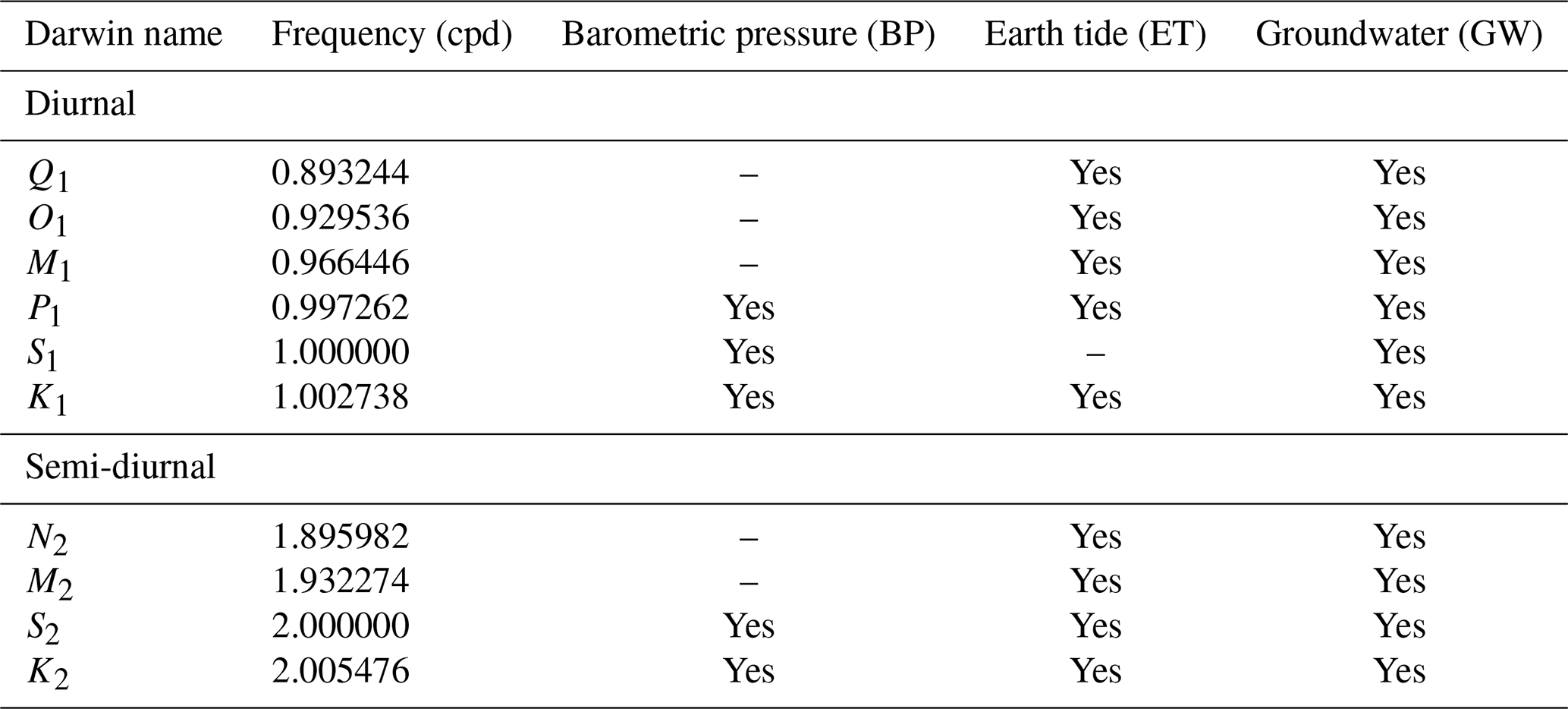
The groundwater response to barometric pressure and gravity changes caused by Earth tides has long been observed and is a powerful yet underutilised tool to passively characterise subsurface systems (McMillan et al., 2019). While atmospheric pressure changes act as a load on the subsurface, and its groundwater pressure response can be related to compressible properties of the formation (e.g. Clark, 1967; Davis and Rasmussen, 1993), Earth tides cause areal strain, resulting in small pore pressure changes (e.g. Bredehoeft, 1967; van der Kamp and Gale, 1983). The main research focus has long been the removal of both signals from the groundwater pressure in order to better understand and quantify processes such as pumping tests or recharge (e.g. Rojstaczer and Agnew, 1989). However, tidal forces are ubiquitous, and their groundwater response can therefore also be utilised to quantify in situ hydro-geomechanical properties (Allègre et al., 2016; Xue et al., 2016). Tidal harmonic components have long been named depending on their frequency (Agnew, 2007). A comprehensive list of the most common components found in groundwater head measurements is summarised in Table 1 (Merritt, 2004). McMillan et al. (2019) reviewed the state of the science, highlighted the potential for such passive approaches and coined the term tidal subsurface analysis (TSA).

Table 1 Overview of the major tidal components found in well water levels (Merritt, 2004; McMillan et al., 2019) grouped by mode (diurnal and semi-diurnal) and ordered by frequency. Columns BP, ET and GW show which component can occur in what type of record. Note: cpd – cycle per day.

Cutillo and Bredehoeft (2011) analysed the groundwater response to both atmospheric pressure changes and Earth tides to quantify hydraulic and elastic properties. They reported that the frequency component S₂ of the groundwater response exhibits a reliable and strong response to Earth tides but could not be used because it is contaminated by atmospheric pressure influences. For this reason, they concentrated their analysis on the Earth tide frequency M₂. Acworth and Brain (2008) and Acworth et al. (2015) used the groundwater response to atmospheric tides to estimate barometric efficiency, infer system confinement and calculate compressible storage. They used the tide frequency S₂ in their work but did not take into account the effects of the phase lags between the Earth, atmospheric and groundwater tides that have been found to introduce errors in the analysis for higher levels of barometric efficiency.

Acworth et al. (2016) published a method which objectively quantifies barometric efficiency (BE) using the groundwater response to atmospheric tides. Their approach considered the impact of phase lags between $S_{\mathrm{2}}^{\mathrm{AT}}$ and $S_{\mathrm{2}}^{\mathrm{ET}}$ in the amplitude response of the groundwater system. Their work demonstrated that (1) the harmonic addition theorem could be used to quantitatively disentangle the groundwater response to both Earth and atmospheric tides (EATs) acting at the same frequency, and (2) a theoretical Earth tide record is sufficient for this purpose. Because Earth tide records can be calculated with very high accuracy for any location on Earth and for time periods of general interest (e.g. McMillan et al., 2019), this has opened the door for the widespread use of common barometric and groundwater pressure measurements (the latter in the form of standard well water levels) to characterise and quantify groundwater systems with little effort. Turnadge et al. (2019) compared different BE estimation methods and concluded that Acworth et al. (2016) delivers robust results.

The method by Acworth et al. (2016) is based on the assumption that the borehole water level is representative of subsurface pore pressure, i.e. there is an instantaneous and undamped response. Under such conditions, only the phase difference between the theoretical Earth and atmospheric tide drivers is required to correct the groundwater response amplitude. However, it has been established that the well water level response to Earth tide forces also depends on the hydraulic properties of the aquifer and well geometry (Bredehoeft, 1967; Gieske and De Vries, 1985; Hsieh et al., 1987) and vadose zone air transport for conditions that are not confined (Rojstaczer, 1988; Allègre et al., 2016; Xue et al., 2016). In fact, the amplitude and phase responses to Earth tides embedded in well water levels have been used to quantify subsurface hydraulic properties (e.g. Hsieh et al., 1987; Ritzi et al., 1991; Xue et al., 2016). Hsieh et al. (1987) reports an average phase shift of −12^∘ between the M₂ Earth tide potential and its well water level response. Consequently, an instantaneous and undamped groundwater response to Earth tides is not always a given and phase delays must be also considered when quantifying BE${}_{S_{\mathrm{2}}}$ from the groundwater response to atmospheric tides.

In this technical note, we generalise the method by Acworth et al. (2016) by more completely disentangling the groundwater response to EATs in the frequency domain. We then illustrate the interpretative value of this new approach, using an example atmospheric pressure and borehole water level record that is strongly affected by EATs, followed by a verification of our results, using the well's barometric response function calculated in the time domain.

2 A generalised frequency domain method

2.1 Complete tidal disentanglement

Since the extension of the method published in Acworth et al. (2016) to a generalised approach requires consideration of both the amplitudes and phases, we use complex numbers (denoted with a hat) for improved clarity. The complex numbers can be expressed with their real and imaginary components as follows:

$$\begin{array}{}\text{(1)}& {\widehat{z}}_c=a_c+b_{c}i=A_c{e}^{i{\mathrm{\Phi }}_c},\end{array}$$

where a_c and b_c are the real and imaginary parts, respectively. $i=\sqrt{-\mathrm{1}}$, following the standard definition. The complex coefficients are related to harmonic amplitudes and phases as follows:

$$\begin{array}{}\text{(2)}& A_c=\mathrm{abs}\left({\widehat{z}}_c\right)=\sqrt{a_c^{\mathrm{2}}+b_c^{\mathrm{2}}},\end{array}$$

and

$$\begin{array}{}\text{(3)}& {\mathrm{\Phi }}_c=\arg \left({\widehat{z}}_c\right)=\arg \left[{\displaystyle \frac{a_c}{b_c}}\right],\end{array}$$

where the results within $-\mathit{\pi }\le {\mathrm{\Phi }}_c\le \mathit{\pi }$.

Throughout this paper, subscripts refer to the considered tidal components c, i.e. M₂ (1.93227 cpd) and S₂ (2 cpd). Superscripts stand for the measured parameter, i.e. GW stands for groundwater pressure head (measured as borehole water level and generally only required as a relative measurement), AT is atmospheric pressure (as water head equivalent) and ET is Earth tide (here, we use strain). Importantly, GW.ET and GW.AT represent the disentangled groundwater components response to Earth and atmospheric tides, respectively.

The method by Acworth et al. (2016) can be generalised to allow a complete disentanglement of Earth and atmospheric tide influences from the groundwater response as follows:

1. The complex groundwater response to the Earth-tide-only driver for the M₂ (1.93227 cpd) component is compared to the complex, theoretical Earth tide generated for the well geo-location, time and duration. Theoretical Earth tides can be calculated using software packages such as ETERNA (Wenzel, 1996), PyGTide (Rau, 2018) (which utilises the latest tidal catalogue), Baytap08 (Agnew, 2008) or TSoft (Van Camp and Vauterin, 2005) (which was originally designed to analyse gravity records). Records for the theoretical Earth tide potential or gravity variations are highly accurate and avoid the need for measurements (McMillan et al., 2019).

2. For some tidal components, for example S₂ (2.0 cpd), the well water level responds to both Earth and atmospheric tides. The groundwater response magnitude to Earth tides only, for example at frequency M₂ (1.93227 cpd), is assumed to be the same as for S₂ because the frequencies are very close. Consequently, the S₂ groundwater response to Earth tides alone can be calculated using the following:

   $$\begin{array}{}\text{(4)}& {\widehat{z}}_{S_{\mathrm{2}}}^{\mathrm{GW}.\mathrm{ET}}={\displaystyle \frac{{\widehat{z}}_{M_{\mathrm{2}}}^{\mathrm{GW}}}{{\widehat{z}}_{M_{\mathrm{2}}}^{\mathrm{ET}}}}{\widehat{z}}_{S_{\mathrm{2}}}^{\mathrm{ET}}.\end{array}$$

3. Since the measured well water level response for S₂ contains a harmonic combination of both Earth and atmospheric tides, in the following (McMillan et al., 2019):

   $$\begin{array}{}\text{(5)}& {\widehat{z}}_{S_{\mathrm{2}}}^{\mathrm{GW}}={\widehat{z}}_{S_{\mathrm{2}}}^{\mathrm{GW}.\mathrm{ET}}+{\widehat{z}}_{S_{\mathrm{2}}}^{\mathrm{GW}.\mathrm{AT}},\end{array}$$

   the complex response to atmospheric tides alone can be calculated as follows:

   $$\begin{array}{}\text{(6)}& {\widehat{z}}_{S_{\mathrm{2}}}^{\mathrm{GW}.\mathrm{AT}}={\widehat{z}}_{S_{\mathrm{2}}}^{\mathrm{GW}}-{\widehat{z}}_{S_{\mathrm{2}}}^{\mathrm{GW}.\mathrm{ET}}={\widehat{z}}_{S_{\mathrm{2}}}^{\mathrm{GW}}-{\displaystyle \frac{{\widehat{z}}_{M_{\mathrm{2}}}^{\mathrm{GW}}}{{\widehat{z}}_{M_{\mathrm{2}}}^{\mathrm{ET}}}}{\widehat{z}}_{S_{\mathrm{2}}}^{\mathrm{ET}}.\end{array}$$

   Unfortunately, Eq. (6) does not have a simplified expression consisting only of real valued numbers or functions.

It is important to note that our extended approach given in Eqs. (4)–(6) is correct irrespective of any processes that may affect the subsurface strain response to the stress induced by Earth tides. For example, delays may result from the physical characteristics of the aquifer borehole system but will be very similar for M₂ and S₂ because the frequencies are so close together. The theoretical Earth tide record merely helps to determine the absolute amplitudes and phases of the Earth tide response at S₂ by accounting for the differences between the complex M₂ and S₂ determined from the theoretical Earth tide record to the absolute one at M₂ measured in the well. The approach extends the method developed by Acworth et al. (2016) because it considers all the signal phases in addition to their amplitudes. Since the inference of the well response to Earth tides is relative, the disentanglement can be done with any theoretical Earth tide signal, e.g. potentials, gravity variations or estimated strains.

2.2 Relationship between borehole water levels and subsurface pore pressure

Acworth et al. (2016) assumed that the groundwater pressure head (i.e. the well water level) is representative of the subsurface pore pressure, i.e. an instantaneous and undamped response. However, calculation of the true BE based on subsurface pore pressure (outside of the well screen) requires a closer look at this relationship. Since tidal components comply well with harmonic functions, we can invoke the assumption that there is harmonically varying flow between the formation and the well (e.g.  Bredehoeft, 1967; Hsieh et al., 1987; Rojstaczer, 1988). This groundwater flow problem has been solved analytically for confined (Hsieh et al., 1987) and semi-confined (i.e. situations with vertical leakage through an overlying aquitard) (Rojstaczer, 1988) conditions (see Appendix A). For the pressure relationship between subsurface and well water level, an amplitude ratio can be defined as follows:

$$\begin{array}{}\text{(7)}& A_c^r=\mathrm{abs}\left[{\displaystyle \frac{{\widehat{z}}_c^{\mathrm{GW}}}{{\widehat{z}}_c^{\mathrm{PP}}}}\right]=\mathrm{abs}\left[\widehat{H}(f_c,T,S,r_{\mathrm{wc}},r_{\mathrm{ws}})\right].\end{array}$$

Furthermore, a phase shift can be formulated as follows:

$$\begin{array}{}\text{(8)}& \mathrm{\Delta }{\mathit{\varphi }}_c=\arg \left[{\displaystyle \frac{{\widehat{z}}_c^{\mathrm{GW}}}{{\widehat{z}}_c^{\mathrm{PP}}}}\right]=\arg \left[\widehat{H}(f_c,T,S,r_{\mathrm{wc}},r_{\mathrm{ws}})\right].\end{array}$$

Here, the subscript c depicts any tidal component with distinct frequency. Superscripts GW and PP stand for well water level and subsurface pore pressure, respectively. The complex analytical function $\widehat{H}$ is given in Appendix A and depends on the variables r_wc and r_ws, which are the radius of the well casing and screen, respectively. b is the screen length. $T=K\cdot b$ and $S=S_{\mathrm{s}}\cdot b$ are the transmissivity and storativity of the formation located along the well screen (Hsieh et al., 1987).

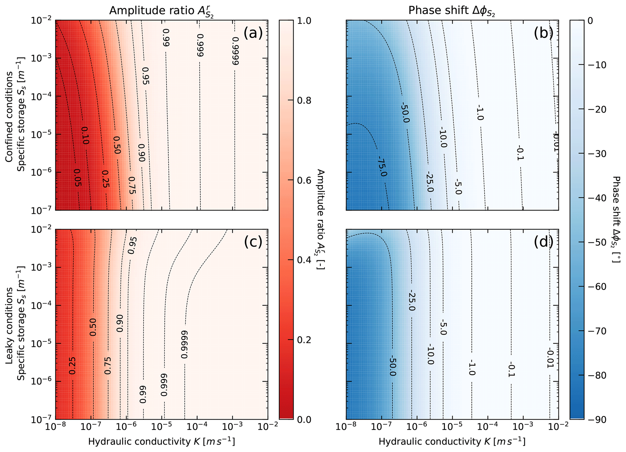
Figure 1 Amplitude ratio and phase shift relationship between subsurface pore pressure and well water level for harmonic forcing under fully confined conditions (a, b) and vertical water leakage under semi-confined conditions (c, d). The leaky aquitard has $K^{\prime }=\mathrm{5}\times {\mathrm{10}}^{-\mathrm{5}}$ m/s and $b^{\prime }=\mathrm{2}$ m. The plots are calculated for a hypothetical well with radius of 25 mm and screen length of 1 m and realistic ranges of hydraulic conductivity and specific storage.

Figure 1 shows the amplitude ratio and phase shift calculated for the M₂ Earth tide component (1.93227 cpd) and a hypothetical groundwater observation point with radius of 25 mm and screen length of 1 m. For the leaky aquifer solution, we assumed an aquitard with $K^{\prime }=\mathrm{5}\times {\mathrm{10}}^{-\mathrm{5}}$ m/s and vertical thickness of 2 m. We used this value as a worst-case higher limit for an aquitard as the resulting amplitudes and phases provide a contrast to the confined case that is significant enough to visualise. The solutions illustrate that there is a frequency-dependent damping and phase shift in the well water level response to the aquifer pore pressure. Importantly, Fig. 1 highlights the following:

• The strongest modification of the harmonic response occurs for fully confined and not for leaky conditions (Fig. 1).

• both amplitude damping and phase shifts are mainly controlled by the subsurface hydraulic conductivity. For the confined case, $A_{S_{\mathrm{2}}}^r>\mathrm{0.99}$, which means that the relative error is smaller than 1 % for $K>\mathrm{1}\times {\mathrm{10}}^{-\mathrm{5}}$ m/s and is therefore negligible. However, $A_{S_{\mathrm{2}}}^r$ dramatically decreases under lower hydraulic conductivity conditions and must therefore be considered for BE^AT estimations.

• S_s does not significantly affect the well water level response, especially for $K>\mathrm{1}\times {\mathrm{10}}^{-\mathrm{5}}$ m/s. However, the amplitude response to the Earth tide strain is proportional to S_s (Eq. 7).

Using Eqs. (4)–(7), a generalised method for objective BE^AT quantification, using the groundwater response to atmospheric tides, for example at S₂, can be formulated as follows:

$$\begin{array}{}\text{(9)}& {\mathrm{BE}}_{S_{\mathrm{2}}}^{\mathrm{AT}}={\displaystyle \frac{\mathrm{1}}{A_{S_{\mathrm{2}}}^r}}\mathrm{abs}\left[{\displaystyle \frac{{\widehat{z}}_{S_{\mathrm{2}}}^{\mathrm{GW}.\mathrm{AT}}}{{\widehat{z}}_{S_{\mathrm{2}}}^{\mathrm{AT}}}}\right].\end{array}$$

Here, $A_{S_{\mathrm{2}}}^r$ accounts for the damping introduced by the subsurface well system under conditions of low hydraulic conductivity. Due to the closeness of the S₂ and the M₂ frequencies, we can assume that $A_{S_{\mathrm{2}}}^r\approx A_{M_{\mathrm{2}}}^r$.

The tidal disentanglement further enables estimation of the subsurface hydraulic conductivity (K) and specific storage (S_s), using the water level response to Earth tides. A negative phase shift between M₂ and its groundwater response (well water level lags the Earth tide strain) requires horizontal flow in and out of the well and is therefore indicative of confined conditions (Roeloffs et al., 1989; Allègre et al., 2016; Xue et al., 2016). In this case, the amplitude and phase response of the well water level to an ET strain component is related (Allègre et al., 2016; Xue et al., 2016) as follows:

$$\begin{array}{}\text{(10)}& A_{M_{\mathrm{2}}}^e=\mathrm{abs}\left[{\displaystyle \frac{{\widehat{z}}_{M_{\mathrm{2}}}^{\mathrm{GW}}}{{\widehat{z}}_{M_{\mathrm{2}}}^{\mathrm{ET}}}}\right]={\displaystyle \frac{A_{M_{\mathrm{2}}}^r}{S_{\mathrm{s}}}},\end{array}$$

(with aerial strain sensitivity equivalent to Eq. (A12) in Appendix A) and in the following:

$$\begin{array}{}\text{(11)}& \mathrm{\Delta }{\mathit{\varphi }}_{M_{\mathrm{2}}}=\arg \left[{\displaystyle \frac{{\widehat{z}}_{M_{\mathrm{2}}}^{\mathrm{GW}}}{{\widehat{z}}_{M_{\mathrm{2}}}^{\mathrm{ET}}}}\right]\end{array}$$

(which is equivalent to Eq. A13 in Appendix A). A positive phase shift is indicative of vertical water movement and semi-confined conditions (Roeloffs et al., 1989; Xue et al., 2016). We note that the concept of BE describes a surface load sharing between matrix and pore water, which only exists under semi-confined to confined conditions, and that values of BE do not necessarily indicate the state of confinement (Turnadge et al., 2019).

2.3 Extraction of tidal components using harmonic least squares

The first step towards tidal disentanglement is to extract the tidal harmonics from the time series. Since the frequencies of the main tidal components are well known (e.g. McMillan et al., 2019), a harmonic least squares (HALSs) estimation can be applied as follows (Agnew, 2007):

$$\begin{array}{}\text{(12)}& \underset{a_c,b_c}{min}\sum _{n=\mathrm{1}}^N{\left[y_n\left(t_n\right)-\sum _{c=\mathrm{1}}^C\left[a_c\cos \left(\mathrm{2}\mathit{\pi }{f}_c{t}_n\right)+b_c\sin \left(\mathrm{2}\mathit{\pi }{f}_c{t}_n\right)\right]\right]}^{\mathrm{2}}.\end{array}$$

Here, N is the number of discrete samples, y_n(t_n) is the sample value at time t_n, and C is the total number of tidal components c with frequency f_c. Table 1 shows the nine strongest tidal components that are generally observable in groundwater pressure measurements (Merritt, 2004; McMillan et al., 2019) and are required for finding the best fit using Eq. (12). The coefficients a_c and b_c from Eq. (12) serve to derive the complex numbers representing each tidal constituent using Eq. (1). We further calculate the uncertainties of amplitudes and phases by propagating the covariances obtained from HALSs fitting (Eq. 12), using Eqs. (2) and (3). For details, refer to Appendix C.

Before extracting tidal harmonics, lower frequency variations should be removed. We suggest first applying a de-trending filter with a cut-off frequency of f<0.5 cpd. This improves the least squares approximation. It is important to note that the components used in the regression have to be customised for barometric pressure (BP), Earth tides (ET) and groundwater pressure head (GW) according to this table. For example, S₁ is only contained in BP. This list is based on the findings by Merritt (2004) and McMillan et al. (2019).

3 Application

The three BE^AT examples illustrated in Acworth et al. (2016) show a limited impact of Earth tides relative to those of the atmospheric tides, resulting in a small magnitude correction at S₂. To illustrate our new tidal disentanglement approach, we deliberately use a well water level record in which the Earth tide influence exceeds that of the atmospheric tides. This record originates from the well of BLM-1 in Death Valley (California, USA; WGS84; −116.471360^∘ longitude, 36.408130^∘ latitude; height – 688 m; casing and screen radius – 0.127 m; screen length – 106 m), which provided data for a previous analysis (Cutillo and Bredehoeft, 2011). The data set used here was recorded in the same well but at a later time. The data set was sampled at 15 min intervals (96 samples per day).

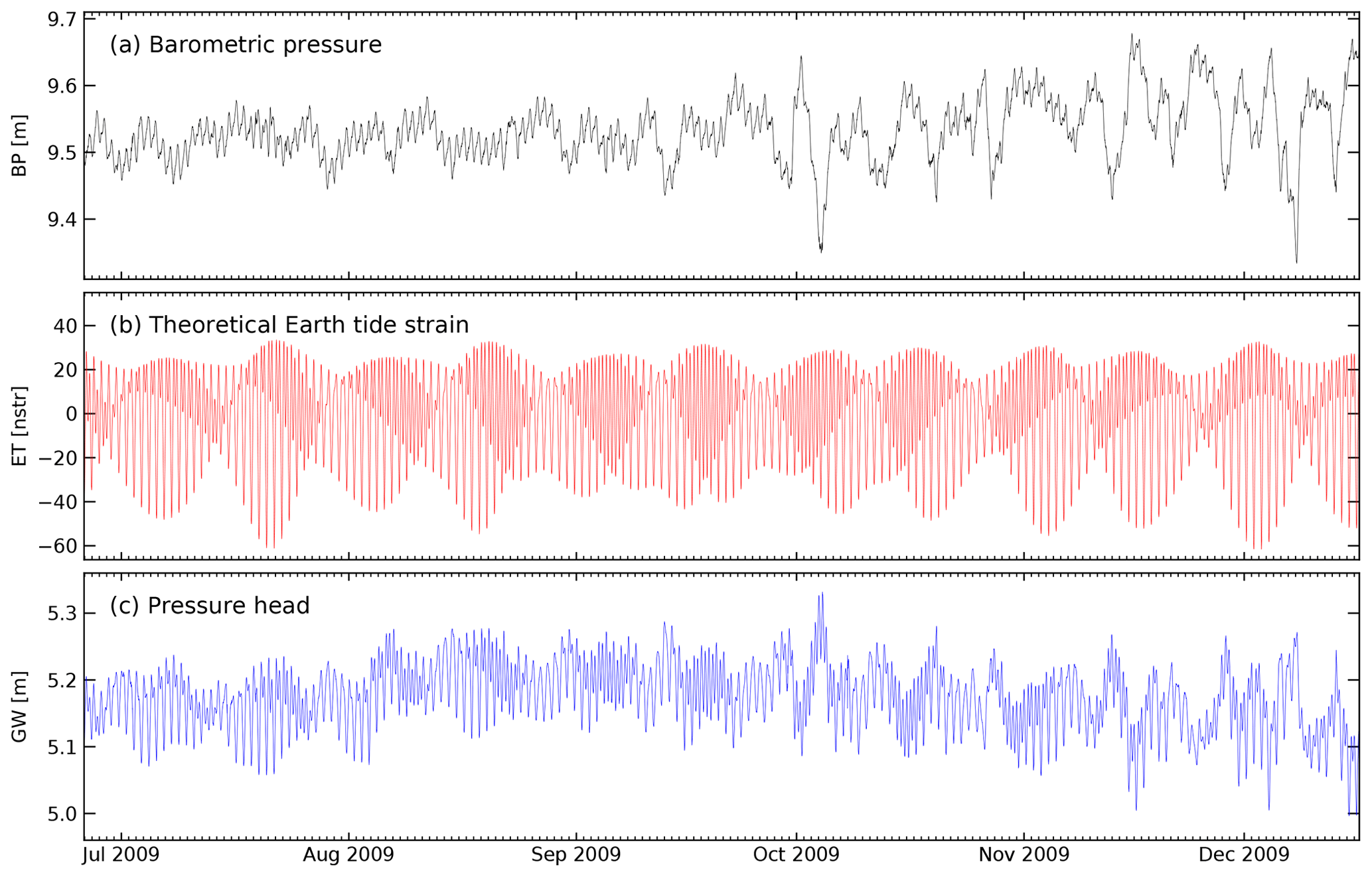
Figure 2 Time series of (a) barometric pressure (BP). (b) Theoretical Earth tide strains (ET) were calculated for the same duration and sampling rate and the well's geo-location using PyGTide (Rau, 2018) and (c) well water levels (GW), as measured in the well BLM-1 in Death Valley (California, USA). The vertical axes for BP and GW are limited to the same range for a visual comparison.

Figure 2 shows the barometric pressure (BP; black line, converted to pressure head equivalent), groundwater pressure head (GW; blue line, as measured in the well) and Earth tide strains (ET; red line) for BLM-1 over a time period of almost 6 months (25 June to 16 December 2009). The Earth tide strains were calculated using the Python package PyGTide (Rau, 2018) for the same time period and sampling frequency as the pressure measurements. It is interesting to note that both Earth tide and atmospheric pressure signatures are clearly visible in the groundwater response. In fact, the impact of both atmospheric pressure and Earth tide strains on the borehole water level is obvious just by looking at the raw data set.

Figure 3 (a) A comparison of groundwater (GW) amplitudes for the interval $\mathrm{0.8}\le f\le \mathrm{2.2}$ cycle per day (cpd) derived using the general harmonic least squares estimation (Eq. 12) and the standard fast Fourier transform. (b) Amplitudes and phases of the most common tidal components in groundwater (GW), barometric pressure (BP) and Earth tides (ET) determined using harmonic least squares estimation. Note that horizontal and vertical error bars show the uncertainty of 1 standard deviation (Appendix C).

As a next step, we extracted the tidal harmonic components from all three time series (BP, ET and GW in Fig. 2) using the harmonic least squares estimation approach described in Sect. 2.3. Figure 3a shows the estimated amplitudes of the tidal components compared to a Fourier amplitude spectrum of the groundwater record. This example illustrates that separating tidal components with close-by frequencies is a clear challenge for the Fourier transform, even when the record duration is longer than that recommended by Acworth et al. (2016). It further highlights the well-known fact that spectral leakage can lead to errors in estimating the properties of the harmonic components (e.g. Tary et al., 2014).

Figure 3b maps the amplitudes of the tidal components (Table 1) extracted from the original time series depicted in Fig. 2 against their phases. As expected, the strongest impact stems from the Earth-tide-only component M₂. It is interesting to observe the similarity in the groundwater response magnitudes for all other Earth tide components, e.g. K₁, O₁, N₂, Q₁ and M₁ (in decreasing order of impact). It is apparent that, at frequencies for which the groundwater record is influenced by both Earth and atmospheric tides, there is a substantial misalignment in amplitudes and phases of these components in groundwater in comparison to the forcing signals, e.g. see S₂ or S₁.

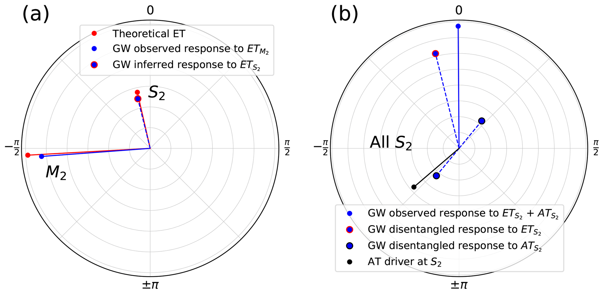
Figure 4 Polar plots showing amplitudes and phases derived from the fitting coefficients using Eqs. (1)–(3). (a) Results of the complex inference of the well response to Earth tides at S₂ from the response at M₂ (Eq. 4). (b) Harmonic disentanglement of the well response to atmospheric tides at S₂ (Eq. 6). In (a), the Earth tide magnitude is scaled to improve comparison with the groundwater response.

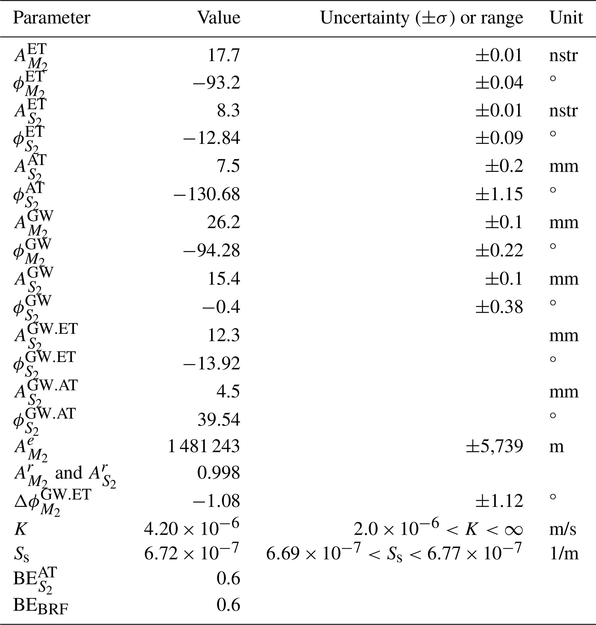
To illustrate the tidal disentanglement, we use polar plots to visualise the key components. Figure 4a shows the amplitude and phase of the M₂ component present in ET and GW. We apply the approach developed in Sect. 2.1 to infer the S₂ response in the well that is caused by the Earth tides alone, using the theoretical Earth tide strains (note that the ET magnitude is scaled to improve comparison). Figure 4b shows the atmospheric tide driver at S₂, the combined well water level response to EAT, the inferred groundwater response to S₂ and the disentangled S₂ response to atmospheric tides. All parameters and uncertainties calculated in this work are summarised in Table 2.

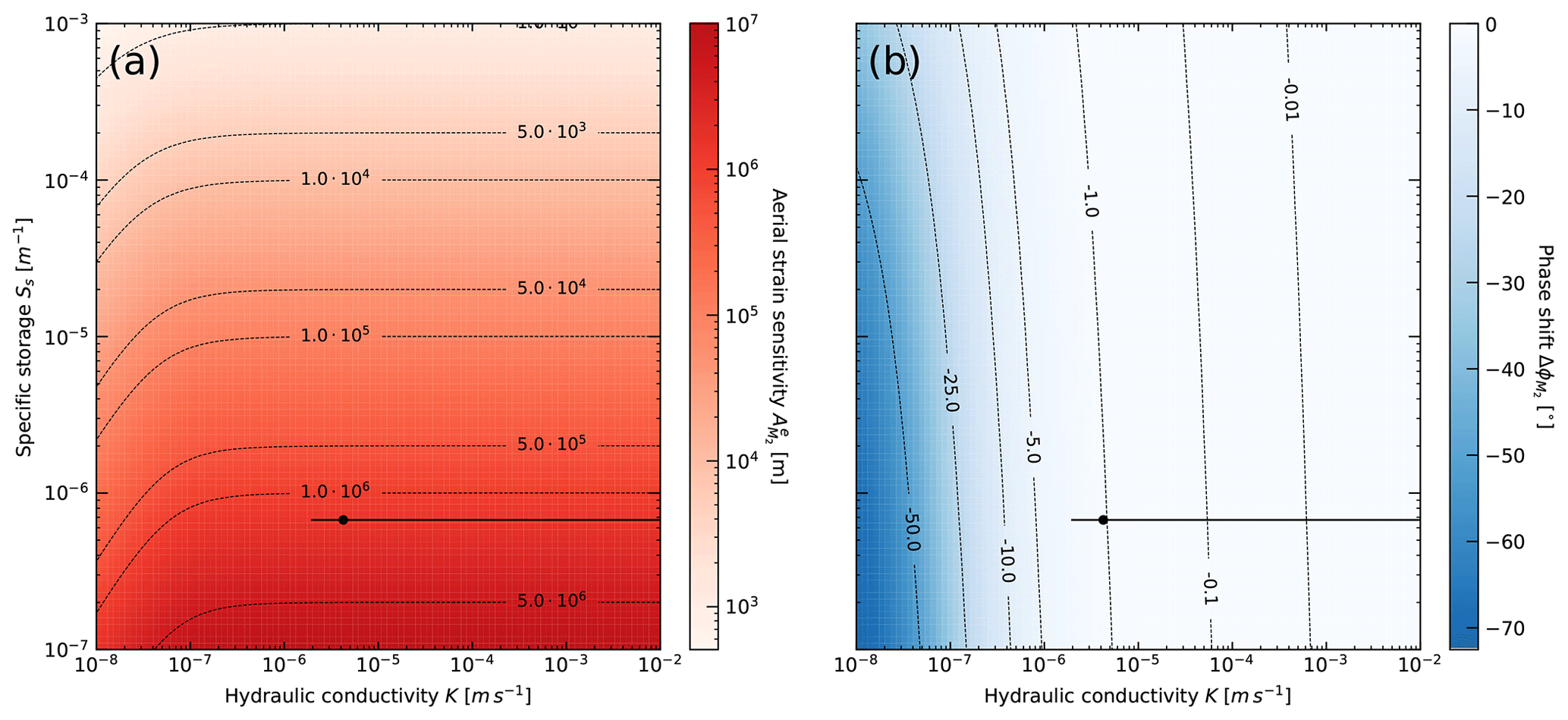
Figure 5 Well water level response to pore pressure for BLM-1 (well radius of 0.127 m and length of 106 m) and S₂ frequency (2.0 cpd). Black dots represent the results for this well found by least squares fitting of the amplitude and phase response to the analytical solutions by Hsieh et al. (1987). The horizontal and vertical (not visible) black lines depict the property ranges as a result of uncertainties in the aerial strain sensitivity and phase difference.

To account for the amplitude damping and phase shifting of the well in response to the harmonic pore pressure changes, we have used the dimensions of the well BLM-1 (see previous details) to calculate the solution space of the analytical solution for confined conditions (Appendix A) for the M₂ frequency and for realistic limits of hydraulic conductivity ($\mathrm{1}\times {\mathrm{10}}^{-\mathrm{8}}<K<\mathrm{1}\times {\mathrm{10}}^{-\mathrm{2}}$ m/s) and specific storage ($\mathrm{1}\times {\mathrm{10}}^{-\mathrm{7}}<S_{\mathrm{s}}<\mathrm{1}\cdot {\mathrm{10}}^{-\mathrm{3}}$ 1/m). The aerial strain sensitivity and phase shift between Earth tides and well response to M₂ is shown in Fig. 5. We further used Eqs. (10) and (11) to estimate the hydraulic conductivity as $K\approx \mathrm{4.2}\times {\mathrm{10}}^{-\mathrm{6}}$ m/s (ranging from $\mathrm{2.0}\times {\mathrm{10}}^{-\mathrm{6}}$ to impossibly high values) and specific storage as $S_{\mathrm{s}}\approx \mathrm{6.7}\times {\mathrm{10}}^{-\mathrm{7}}$ 1/m (ranging from $\mathrm{6.69}\times {\mathrm{10}}^{-\mathrm{7}}$ to $\mathrm{6.77}\times {\mathrm{10}}^{-\mathrm{7}}$ 1/m), which is representative for the materials along the well screen from the groundwater response to Earth tides (note the black annotations in Fig. 5). The S_s falls within the poroelastic limits determined by (Rau et al., 2018).

The damping of the amplitude in the well in this case is only $A_{M_{\mathrm{2}}}^r\approx \mathrm{0.998}$, which differs to the aquifer pore pressure by merely ≈0.2 %. It is important to note the high sensitivity to phase differences, i.e. small changes in $\mathrm{\Delta }{\mathit{\varphi }}_{M_{\mathrm{2}}}$ can cause large changes in the value of K (Eq. A13 and Fig. 5b). However, we note that as the sensitivity of the phase difference $\mathrm{\Delta }{\mathit{\varphi }}_{M_{\mathrm{2}}}$ to K drastically reduces in lower permeability settings (Fig. 1b), the confidence in K values will increase. Conveniently, this is also the value range where the amplitude response is most affected (Fig. 1a), allowing confidence in the robustness of our new BE${}_{S_{\mathrm{2}}}$ estimation approach for the investigated property ranges.

Figure 6 (a) Borehole pressure head (GW) measured and corrected for barometric and Earth tide influences. (b) Barometric response function (BRF) and BE_BRF calculated using the records shown in Fig. 2 and the approach summarised in Appendix B.

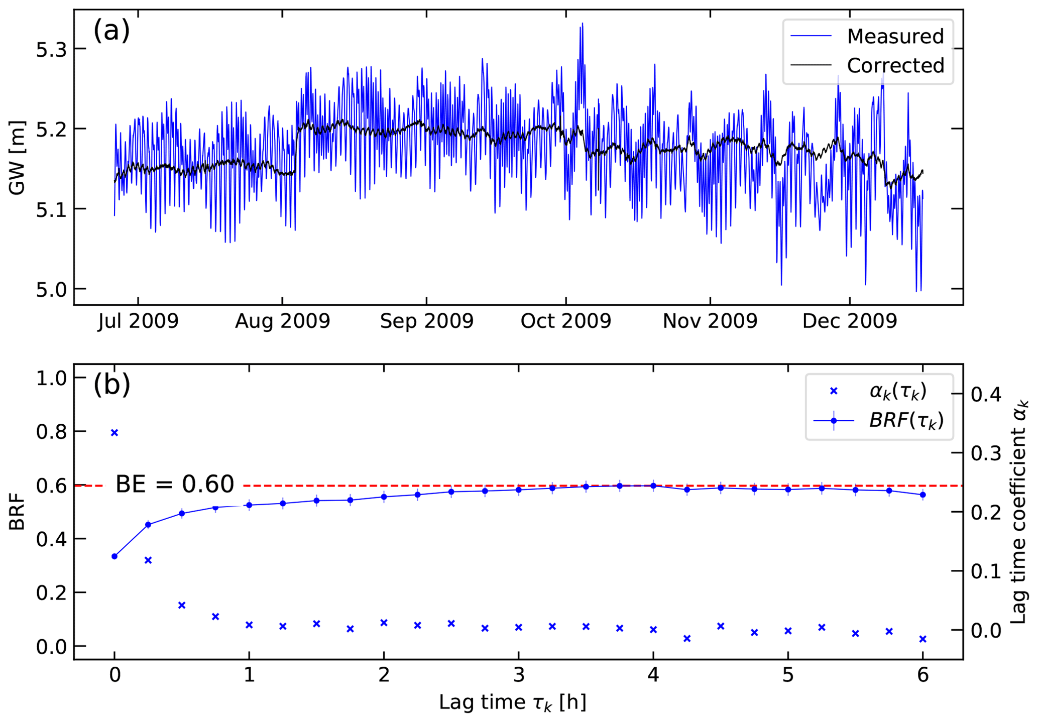
Using Eq. (9), we calculate a BE${}_{S_{\mathrm{2}}}=\mathrm{0.60}$ from the disentangled groundwater response to atmospheric tides at S₂ frequency. This is significantly different to the BE${}_{S_{\mathrm{2}}}=\mathrm{1.29}$ that results from using the method by Acworth et al. (2016). The latter is clearly erroneous, since it is larger than one, owing to the limited phase correction and leading to an incomplete disentanglement of the groundwater response to EATs. To verify our results, we independently calculated BE_BRF for this location using the well-established barometric response function (BRF) approach developed and illustrated previously (a brief summary of the theory is given in Appendix B; Rasmussen and Crawford, 1997; Spane, 2002; Toll and Rasmussen, 2007; Butler et al., 2011). The asymptotic value of the BRF at larger delay times represents confined conditions. The results further exhibit an exponential increase in the BRF over lag time (Fig. 6b). This is typical for water exchange controlled by the subsurface hydraulic conductivity where the shorter the lag time the stronger the deviation from BE (Rasmussen and Crawford, 1997), and it complies well with the frequency-dependent relationship shown in Fig. 1 (Rojstaczer, 1988; Rojstaczer and Agnew, 1989).

The BRF-based BE_BRF≈0.60 exactly matches that calculated using Eq. (9), confirming the robustness of the tidal disentanglement methodology we present in this work. The BRF is able to adequately remove the Earth and atmospheric influences on the measured groundwater levels (Fig. 6a). While BRFs are capable of indicating system confinement and estimating BE, they have not been used for estimating hydraulic properties.

Table 2 Summary of the parameters, values and uncertainties calculated in this work.

The negative phase shift between Earth tides and groundwater pressure ($\mathrm{\Delta }{\mathit{\varphi }}_{M_{\mathrm{2}}}^{\mathrm{GW}.\mathrm{ET}}=-\mathrm{1.1}{}^{\circ }$; see Fig. 4a) can be interpreted as horizontal flow between the subsurface and the well, which occurs under confined conditions (Roeloffs et al., 1989; Xue et al., 2016). Confined conditions can also be interpreted from the fact that the BRF time values reach a maximum value that is representative of the BE (Rasmussen and Crawford, 1997). Since this means that the well is screened in the confined zone, vertical loading due to atmospheric tides should also predominantly induce horizontal flow between the subsurface and the well with the same phase difference as given in response to Earth tides but considering the typical 180^∘ (Fig. 4b) difference related to the subsurface stress balance (Rojstaczer, 1988; Acworth et al., 2016). In fact, $\mathrm{\Delta }{\mathit{\varphi }}_{S_{\mathrm{2}}}^{\mathrm{GW}.\mathrm{AT}}=-\mathrm{9.8}{}^{\circ }$, which is also negative and very close to the phase delay in response to Earth tides.

Previous works have reported that a phase difference of 180^∘ between the atmospheric tides and the groundwater response at S₂ can be used to indicate confinement (Acworth et al., 2016, 2017). However, this did not consider the fully disentangled groundwater response to atmospheric tides. Furthermore, Rojstaczer (1988) has illustrated that the well response to barometric pressure depends on a number of processes accounting for the pressure propagation between surface and well, resulting in a frequency-dependent response of the borehole water level to barometric forcing. We propose that a combination of $\mathrm{\Delta }{\mathit{\varphi }}_{M_{\mathrm{2}}}$ and $\mathrm{\Delta }{\mathit{\varphi }}_{S_{\mathrm{2}}}$ could be diagnostic of the subsurface conditions at the borehole location. For example, a negative $\mathrm{\Delta }{\mathit{\varphi }}_{M_{\mathrm{2}}}$ is indicative of horizontal flow occurring under confined conditions for which $\mathrm{\Delta }{\mathit{\varphi }}_{S_{\mathrm{2}}}$ should equally be shifted to account for the 180^∘ phase difference. A positive $\mathrm{\Delta }{\mathit{\varphi }}_{M_{\mathrm{2}}}$ has been attributed to vertical water movement (Hanson and Owen, 1982; Roeloffs et al., 1989; Xue et al., 2016) under which the response of $\mathrm{\Delta }{\mathit{\varphi }}_{S_{\mathrm{2}}}$ could become diagnostic of the vertical pressure propagation and vadose zone properties (Rojstaczer, 1988). However, further research is required to develop a robust approach for detecting the confinement status at a particular frequency.

4 Conclusions

We present a frequency domain method to disentangle the groundwater response to Earth and atmospheric tides. It is a more general solution than that previously presented by Acworth et al. (2016) since it is also applicable to subsurface environments with lower hydraulic conductivities, where measurable damping and time lags between formation pressure changes and well water level responses may be present. The approach only requires simultaneous records of barometric and groundwater pressure head in combination with theoretical Earth tide potential, gravity or strain variations, which are either standard measurements or can be calculated for any borehole geo-position using readily available software. Our novel approach exploits the fact that the complex harmonic components can be determined for each variable, i.e. barometric pressure, borehole water level and Earth tides from which subsurface flow direction (horizontal vs. vertical) in response to stresses allows the inference of confinement, estimation of barometric efficiency (BE), hydraulic conductivity and specific storage. We show that BE calculation using the borehole water level response to atmospheric tides may be substantially influenced by the hydraulic conductivity of the materials surrounding the well screen where $K<\mathrm{1}\times {\mathrm{10}}^{-\mathrm{5}}$ m/s.

Our method enables an improved and rapid estimation of BE in general but especially for cases where the borehole water level is strongly influenced by Earth tides. Under such conditions, the influence of the phase difference between Earth tides and its groundwater response also has to be considered when revealing the atmospheric tide embedded in the S₂ component of groundwater head measurements. The generalised solution further improves existing approaches and provides a next step towards a more reliable quantification of subsurface hydro-geomechanical properties using the groundwater response to Earth and atmospheric tides (McMillan et al., 2019).

Appendix A: Well water level response to aquifer pore pressure

The following differential equation describes water flow in and out of a well under semi-confined (leaky) conditions:

$$\begin{array}{}\text{(A1)}& {\displaystyle \frac{{\mathit{\delta }}^{\mathrm{2}}s}{\mathit{\delta }{r}^{\mathrm{2}}}}+{\displaystyle \frac{\mathrm{1}\mathit{\delta }s}{r\mathit{\delta }r}}-{\displaystyle \frac{K^{\prime }s}{b^{\prime }Kb}}={\displaystyle \frac{S_{\mathrm{s}}\mathit{\delta }s}{K\mathit{\delta }t}}.\end{array}$$

Here, s is the drawdown in the aquifer, r is the radius from the centre of the well, K and S_s are the hydraulic conductivity and specific storage of the aquifer, b is the aquifer thickness (here assumed to be the length of the well screen), and K^′ and b^′ are the hydraulic conductivity and thickness of the aquitard overlying the aquifer. Rojstaczer (1988) has solved this equation for harmonically varying flow in and out of the well with the following boundary conditions:

$$\begin{array}{}\text{(A2)}& s(\mathrm{\infty },t)=\mathrm{0},\end{array}$$

and

$$\begin{array}{}\text{(A3)}& \underset{r\to \mathrm{0}}{lim}{\displaystyle \frac{r\mathit{\delta }s}{\mathit{\delta }r}}={\displaystyle \frac{\mathit{\omega }{r}_{\mathrm{ws}}^{\mathrm{2}}\widehat{x}}{\mathrm{2}Kb}}\sin \left(\mathit{\omega }t\right).\end{array}$$

The solution for the drawdown just outside the well screen r_ws is as follows:

$$\begin{array}{}\text{(A4)}& {\widehat{s}}_w={\widehat{x}}_{\mathrm{0}}\cdot \widehat{G},\end{array}$$

and

$$\begin{array}{}\text{(A5)}& \begin{array}{rl}\widehat{G}& =\mathrm{0.5}i\cdot W\cdot K_{\mathrm{0}}[{\left[W^{\mathrm{2}}\left[S^{\mathrm{2}}+{\displaystyle \frac{\mathrm{1}}{q^{\mathrm{2}}}}\right]\right]}^{\mathrm{0.25}}\\ & \cdot \exp \left[\mathrm{0.5}i\left[\mathrm{atan}\left(qS\right)\right]\right]\left.\right]\cdot \exp \left(i\mathit{\omega }t\right).\end{array}\end{array}$$

In the following:

$$\begin{array}{}\text{(A6)}& W={\displaystyle \frac{\mathit{\omega }{r}_{\mathrm{ws}}^{\mathrm{2}}}{Kb}}\end{array}$$

and

$$\begin{array}{}\text{(A7)}& q={\displaystyle \frac{\mathit{\omega }{b}^{\prime }}{K^{\prime }}}\end{array}$$

and

$$\begin{array}{}\text{(A8)}& \mathit{\omega }=\mathrm{2}\mathit{\pi }f.\end{array}$$

Furthermore, K₀ is the modified Bessel function of the second kind of order zero.

The fluctuating water level and the drawdown are related by the following:

$$\begin{array}{}\text{(A9)}& \widehat{x}={\widehat{h}}_f-{\widehat{s}}_w,\end{array}$$

where $\widehat{x}$ is the borehole water level, $\widehat{h}$ is the subsurface pressure head, and $\widehat{s}$ is the drawdown. Equation (A4) can be substituted into Eq. (A9) to form a complex ratio of the well water level response to changing pore pressure as follows:

$$\begin{array}{}\text{(A10)}& \widehat{H}={\displaystyle \frac{\mathrm{1}}{\mathrm{1}+\widehat{G}}}.\end{array}$$

For fully confined conditions, when $K^{\prime }\to \mathrm{0}$ and $b^{\prime }\to \mathrm{\infty }$, then the third term in Eq. (A1) becomes negligible, and the analytical solution becomes the same as that solved by Hsieh et al. (1987). Hsieh et al. (1988) have shown that, in the following:

$$\begin{array}{}\text{(A11)}& \widehat{h}={\displaystyle \frac{\widehat{\mathit{ϵ}}}{S_{\mathrm{s}}}},\end{array}$$

where ϵ is a strain. Using this relationship, the amplitude ratio and phase shift can be formulated as follows (Xue et al., 2016):

$$\begin{array}{}\text{(A12)}& A_r=\mathrm{abs}\left[{\displaystyle \frac{\widehat{x}}{\widehat{\mathit{ϵ}}}}\right]S_{\mathrm{s}}={\displaystyle \frac{\mathrm{1}}{\sqrt{(E^{\mathrm{2}}+F^{\mathrm{2}})}}},\end{array}$$

and

$$\begin{array}{}\text{(A13)}& \mathrm{\Delta }\mathit{\varphi }=\arg \left[{\displaystyle \frac{\widehat{x}}{\widehat{\mathit{ϵ}}}}\right]=-{\tan }^{-\mathrm{1}}\left[{\displaystyle \frac{F}{E}}\right].\end{array}$$

In the following:

$$\begin{array}{}\text{(A14)}& E=\mathrm{1}-{\displaystyle \frac{\mathrm{2}\mathit{\pi }f{r}_{wc}^{\mathrm{2}}}{\mathrm{2}Kb}}\left[\mathrm{\Psi }\mathrm{Ker}\left[{\mathit{\alpha }}_w\right]+\mathrm{\Phi }\mathrm{Kei}\left[{\mathit{\alpha }}_w\right]\right],\end{array}$$

and

$$\begin{array}{}\text{(A15)}& F={\displaystyle \frac{\mathrm{2}\mathit{\pi }f{r}_{\mathrm{wc}}^{\mathrm{2}}}{\mathrm{2}Kb}}\left[\mathrm{\Phi }\mathrm{Ker}\left[{\mathit{\alpha }}_w\right]-\mathrm{\Psi }\mathrm{Kei}\left[{\mathit{\alpha }}_w\right]\right],\end{array}$$

with

$$\begin{array}{}\text{(A16)}& \mathrm{\Phi }=-{\displaystyle \frac{{\mathrm{Ker}}_{\mathrm{1}}\left[{\mathit{\alpha }}_w\right]+{\mathrm{Kei}}_{\mathrm{1}}\left[{\mathit{\alpha }}_w\right]}{\sqrt{\mathrm{2}}{\mathit{\alpha }}_w\left({\mathrm{Ker}}_{\mathrm{1}}^{\mathrm{2}}\right[{\mathit{\alpha }}_w]+{\mathrm{Kei}}_{\mathrm{1}}^{\mathrm{2}}[{\mathit{\alpha }}_w\left]\right)}},\end{array}$$

and

$$\begin{array}{}\text{(A17)}& \mathrm{\Psi }=-{\displaystyle \frac{Ke{r}_{\mathrm{1}}\left[{\mathit{\alpha }}_w\right]-{\mathrm{Kei}}_{\mathrm{1}}\left[{\mathit{\alpha }}_w\right]}{\sqrt{\mathrm{2}}{\mathit{\alpha }}_w\left({\mathrm{Ker}}_{\mathrm{1}}^{\mathrm{2}}\right[{\mathit{\alpha }}_w]+{\mathrm{Kei}}_{\mathrm{1}}^{\mathrm{2}}[{\mathit{\alpha }}_w\left]\right)}}.\end{array}$$

Here, Ker and Kei are the kelvin functions of order zero, whereas Ker₁ and Kei₁ are the kelvin functions of order one. Finally, in the following:

$$\begin{array}{}\text{(A18)}& {\mathit{\alpha }}_w=\sqrt{{\displaystyle \frac{\mathit{\omega }{S}_{\mathrm{s}}b}{Kb}}}{r}_{\mathrm{ws}}.\end{array}$$

Appendix B: Calculating BE using the barometric response function

The well water level response to barometric pressure forcing in the time domain is referred to as the barometric response function (BRF). A BRF can be used to indicate confinement and estimate barometric efficiency (Rasmussen and Crawford, 1997; Spane, 2002). To account for time delays between changes in barometric pressure and their borehole water level changes, the differences are convoluted, and the time coefficients are determined by least squares regression. The method is as follows (Rasmussen and Crawford, 1997; Butler et al., 2011):

$$\begin{array}{}\text{(B1)}& \underset{{\mathit{\alpha }}_k,{\mathit{\beta }}_k}{min}\sum _{n=\mathrm{0}}^{N-\mathrm{1}}{\left[\mathrm{\Delta }\mathrm{GW}\left(t_n\right)-\sum _{k=\mathrm{0}}^K\left[{\mathit{\alpha }}_k\mathrm{\Delta }\mathrm{BP}(t_n-{\mathit{\tau }}_k)+{\mathit{\beta }}_k\mathrm{\Delta }\mathrm{ET}(t_n-{\mathit{\tau }}_k)\right]\right]}^{\mathrm{2}},\end{array}$$

where ΔGW, ΔBP and ΔET are the changes in borehole water level, barometric pressure, and theoretical Earth tides (potential, gravity or strain), respectively. t_n is the time of sample n, where N is the total number of samples. K is the total number of time lags with relative time τ_k=kΔt. α_k and β_k are the time lag coefficients for the barometric and Earth tide response, respectively. Δt is the sampling period. It is a condition that K≤N. The time-based barometric response function for is calculated as follows:

$$\begin{array}{}\text{(B2)}& \mathrm{BRF}\left({\mathit{\tau }}_k\right)=\sum _{k=\mathrm{0}}^K{\mathit{\alpha }}_k\left({\mathit{\tau }}_k\right).\end{array}$$

According to Rasmussen and Crawford (1997), the BRF(t_k) has a characteristic shape that is indicative of the system's confinement. If a system is confined, then BE can be calculated as follows (Rasmussen and Crawford, 1997):

$$\begin{array}{}\text{(B3)}& \mathrm{BE}=max\left[\mathrm{BRF}\left({\mathit{\tau }}_k\right)\right].\end{array}$$

This time-domain approach can also be used to remove barometric and Earth tide influences from the pressure head time series, for example, to reveal small responses to pumping that are otherwise buried in the natural signals. We note that we do not further interpret the Earth tide lag coefficients β_k in this work.

Appendix C: Amplitude and phase uncertainty estimation

When HALSs optimisation (Eq. 12) is performed, a covariance matrix σ for the fitted coefficients a_c and b_c can be estimated. These can be propagated to obtain standard deviations for the amplitude (Eq. 2) as follows:

$$\begin{array}{}\text{(C1)}& {\mathit{\sigma }}_{A_c}\approx \sqrt{{\left({\displaystyle \frac{a_c}{A_c}}\right)}^{\mathrm{2}}{\mathit{\sigma }}_{a_c}^{\mathrm{2}}+{\left({\displaystyle \frac{b_c}{A_c}}\right)}^{\mathrm{2}}{\mathit{\sigma }}_{b_c}^{\mathrm{2}}+{\displaystyle \frac{\mathrm{2}{a}_c{b}_c}{A_c^{\mathrm{2}}}}{\mathit{\sigma }}_{a_c{b}_c}},\end{array}$$

and for the phase (Eq. 3) as follows:

$$\begin{array}{}\text{(C2)}& {\mathit{\sigma }}_{{\mathit{\varphi }}_c}\approx \sqrt{{\left({\displaystyle \frac{b_c}{a_c^{\mathrm{2}}+b_c^{\mathrm{2}}}}\right)}^{\mathrm{2}}{\mathit{\sigma }}_{a_c}^{\mathrm{2}}+{\left({\displaystyle \frac{-a_c}{a_c^{\mathrm{2}}+b_c^{\mathrm{2}}}}\right)}^{\mathrm{2}}{\mathit{\sigma }}_{b_c}^{\mathrm{2}}-{\displaystyle \frac{\mathrm{2}{a}_c{b}_c}{(a_c^{\mathrm{2}}+b_c^{\mathrm{2}}{)}^{\mathrm{2}}}}{\mathit{\sigma }}_{a_c{b}_c}}.\end{array}$$

This further allows propagation to aerial strain sensitivity as follows:

$$\begin{array}{}\text{(C3)}& {\mathit{\sigma }}_{A_c^{i,j}}\approx \left|A_c^{i,j}\right|\sqrt{{\left({\displaystyle \frac{{\mathit{\sigma }}_{A_c^i}}{A_c^i}}\right)}^{\mathrm{2}}+{\left({\displaystyle \frac{{\mathit{\sigma }}_{A_c^j}}{A_c^j}}\right)}^{\mathrm{2}}},\end{array}$$

and the phase shift as follows:

$$\begin{array}{}\text{(C4)}& {\mathit{\sigma }}_{\mathrm{\Delta }{\mathit{\varphi }}_c^{i,j}}\approx \sqrt{{\mathit{\sigma }}_{{\mathit{\varphi }}_c^i}^{\mathrm{2}}+{\mathit{\sigma }}_{{\mathit{\varphi }}_c^j}^{\mathrm{2}}}.\end{array}$$

Here, the superscripts i and j stand for the two components that are related to each other, e.g. ET or GW.