the Creative Commons Attribution 4.0 License.
the Creative Commons Attribution 4.0 License.
 | 03 Dec 2020
Physics-inspired integrated space–time artificial neural networks for regional groundwater flow modeling
Ali Ghaseminejad
Venkatesh Uddameri
An integrated space–time artificial neural network (ANN) model inspired by the governing groundwater flow equation was developed to test whether a single ANN is capable of modeling regional groundwater flow systems. Model-independent entropy measures and random forest (RF)-based feature selection procedures were used to identify suitable inputs for ANNs. L2 regularization, five-fold cross-validation, and an adaptive stochastic gradient descent (ADAM) algorithm led to a parsimonious ANN model for a 30 691 km2 agriculturally intensive area in the Ogallala Aquifer of Texas. The model testing at 38 independent wells during the 1956–2008 calibration period showed no overfitting issues and highlighted the model's ability to capture both the observed spatial dependence and temporal variability. The forecasting period (2009–2015) was marked by extreme climate variability in the region and served to evaluate the extrapolation capabilities of the model. While ANN models are universal interpolators, the model was able to capture the general trends and provide groundwater level estimates that were better than using historical means. Model sensitivity analysis indicated that pumping was the most sensitive process. Incorporation of spatial variability was more critical than capturing temporal persistence. The use of the standardized precipitation–evapotranspiration index (SPEI) as a surrogate for pumping was generally adequate but was unable to capture the heterogeneous groundwater extraction preferences of farmers under extreme climate conditions.
- Article
(8227 KB) - Full-text XML
- BibTeX
- EndNote


There is a growing recognition that alternative, data-driven model formulations can be employed to better capture nonlinear aquifer response dynamics (Obergfell et al., 2019; Roshni et al., 2019; Rinderer et al., 2018; Adamowski and Chan, 2011; Daliakopoulos et al., 2005). Artificial neural networks (ANNs) are a class of machine learning algorithms that are universal approximators capable of modeling highly nonlinear phenomena (Hornik et al., 1989). ANNs exhibit the ability to capture short-term volatility and long-term persistence effects often seen in groundwater time series data, either explicitly through input specification or implicitly using specific architectures (Principe et al., 2000). As such, ANNs have been widely used to model groundwater level changes at individual wells (Liu et al., 2018; Nizar Shamsuddin et al., 2017; Trichakis et al., 2011; Uddameri, 2007; Nayak et al., 2006) and simultaneously at a group of wells (Mohanty et al., 2015). While forecasting water levels at individual wells is sufficient in certain groundwater applications, capturing the spatiotemporal dynamics of groundwater levels is critical for regional-scale aquifer management.
While regional groundwater flow models continue to be developed using physically based methods that integrate conservation principles and Darcy's law (Anderson et al., 2015; Harbaugh, 2005), attempts have also been made to capture spatiotemporal groundwater behavior using ANNs (Sahoo et al., 2017a, b; Tapoglou et al., 2014; Nourani et al., 2011, 2008). Spatiotemporal modeling of groundwater levels using ANNs is often carried out using a two-stage process. In the first stage, separate ANN models are constructed at individual wells where groundwater level time series data are available. In the second stage, forecasts from these individual wells are regionalized using statistical and geostatistical interpolation methods (Isaaks and Srivastava, 1989; Barnes, 1964).
Two-stage (ANN and interpolation) models for predicting spatiotemporal variability in groundwater levels are conceptually intuitive and pragmatic. However, this approach has limited fidelity to the groundwater system it intends to model. The approach essentially decouples the temporal variations observed at the wells, which is captured by fitting ANNs at individual wells, and the regional-scale spatial variability, which is encapsulated using a geostatistical method. The assumption that spatial and temporal correlations can be decoupled is not fully consistent with conditions in the field, as temporal changes in neighboring wells can locally alter flow paths and affect water level forecasts at a given well (Varouchakis et al., 2019).
As ANNs are universal approximators, it can be hypothesized that a single space–time formulation could conceivably be sufficient to model the regional-scale spatiotemporal water level dynamics. The integration of space–time dynamics into a single ANN architecture allows for the simultaneous characterization of the coupled spatiotemporal dependencies using a parsimonious model formulation. The primary goal of this study is to test this hypothesis by constructing a single space–time ANN model to capture the spatiotemporal variability in groundwater levels noted within a region. Such a model is referred to here as the integrated space–time (IST–ANN for brevity) model. The ANN model development is guided by the governing groundwater flow equation. We recommend that such a physics-inspired model development be followed, as it leads to greater transparency in the development of data-driven modeling exercises which are often dismissed as black boxes. Theoretical considerations for developing IST–ANN models are presented in the paper, and the developed methodology is used to model regional groundwater flow in a portion of the Ogallala Aquifer in the southern High Plains of Texas as an illustrative case study.
2.1 Conceptualization of the IST–ANN architecture
Regional groundwater flow in an aquifer can be modeled using the governing groundwater flow equation, which generically can be stated as follows:
where H is the hydraulic head (L), and Ss is the specific storage of the aquifer (L−1). K is the hydraulic conductivity (LT−1), and is the source and/or sink term (T−1). x, y, and z are perpendicular to the cartesian coordinates, and the x axis is oriented parallel to the direction of flow, and t is the time. Source and/or sink terms include recharge from precipitation, groundwater extractions from wells, exchange of water with surface water bodies (river and lakes) and other point, line, and areal sources and sinks. The solution of Eq. (1), subject to specified initial and boundary conditions, yields values of hydraulic head H at locations denoted by (x, y, and z) and at time (t). A first-order finite-difference formulation of Eq. (1) approximates the partial derivatives with difference equations, and the hydraulic head at any point in space (x, y, and z) and time (t) can be expressed as follows:
As can be seen from Eq. (2), the hydraulic head at (x, y, z, and t) is the sum of the hydraulic head measured at the same location at the previous time step (t−1), and the change in hydraulic head between time t and (t−1) is denoted as . This dependence of current water levels on values measured at previous time steps denotes the persistence of the groundwater level time series at a given location. Equation (3) also indicates that the change in water level is also a function of hydraulic heads at the neighboring cells and can be viewed as spatial dependence effects in the groundwater level time series. Groundwater source and sink terms (Q′) at (x, y, and z) and at time t also affect the hydraulic heads in the aquifer. These source and/or sink terms represent the external stresses imposed on the aquifer. Hydraulic heads also depend upon a vector of aquifer properties (θ). These aquifer properties include hydraulic conductivity (K), specific storage (Ss), and aquifer thickness (H or b, depending on whether the aquifer is confined or unconfined), all of which can vary in space. These terms highlight the dependence of groundwater level time series on intrinsic aquifer characteristics. These aquifer characteristics typically exhibit spatial variability as well.
The governing groundwater flow equation is taken as the starting point for developing integrated space–time artificial neural network (IST–ANN) models. The hydraulic head (H) at a time (t) and at a well located at spatial location (x, y, and z) is assumed to be a function of the lagged hydraulic head () at a given well. While higher order lags are usually neglected in standard finite difference groundwater flow simulators (Harbaugh, 2005), they have been noted to increase the accuracy of finite difference schemes (Mickens, 2005; Farthing et al., 2003).
Equation (3) indicates the groundwater level at a location (x, y, z, and t) is a function of hydraulic head values at neighboring wells. In explicit finite difference schemes, these neighboring well heads at a time (t) are approximated by heads that are previous lag(s) for mathematical simplicity. Such an assumption also becomes necessary for incorporating spatial dependence in feed-forward ANNs to avoid circular input–output relationships. Also, wells (grid locations where heads are computed) are seldom located at regular intervals in real-world monitoring networks (Uddameri and Andruss, 2014). As ANN models are data driven, the nearest neighbors will unlikely be equidistant at all locations of interest. The random well spacing is similar to using a nonuniform finite-difference grid for solving the governing groundwater flow equation. In summary, the governing groundwater flow equation inspires ANN models to include hydraulic heads from neighboring wells as they are likely to have a strong influence on forecasts and to help capture the spatial-dependence structure of the groundwater level time series. A recent study also corroborates that the inclusion of information from neighboring wells improves the predictive abilities of ANN models while forecasting groundwater levels (Amaranto et al., 2019).
2.2 Input specification of regional ANN model
As in physically based modeling, understanding the compatibility between the model and the system it seeks to represent is critical while developing ANN models. Choices for processes to consider, and how to represent them (i.e., parameterization) in the absence of direct measurements, must be carefully ascertained (Oreskes et al., 1994). Data pertaining to source and sink terms are seldom available in practical field applications (Russo and Lall, 2017) and are often estimated using surrogate measures, even in physical groundwater modeling applications. This limitation also affects the development of regional-scale ANN models. However, regional-scale ANN models allow one to directly incorporate surrogate information for sources and sinks as inputs and, thus, eliminate the need to convert them into flux terms needed in physically based models. This convenience removes the need for other empirical models and rules of thumb during the model parameterization process.
The specification of the spatial variability of aquifer parameters (e.g., hydraulic conductivity) is another important consideration and also a major source of subjectivity when parameterizing physically based models (Gómez-Hernández and Gorelick, 1989). Aquifer properties can be directly included in ANN models when available. However, as these properties exhibit spatial variability, it is also possible to capture their effects using location (x, y, and z) coordinates. The use of location coordinates to capture spatial variability is similar to spatial regression approaches that have been used to regionalize groundwater level measurements (Nourani et al., 2008).
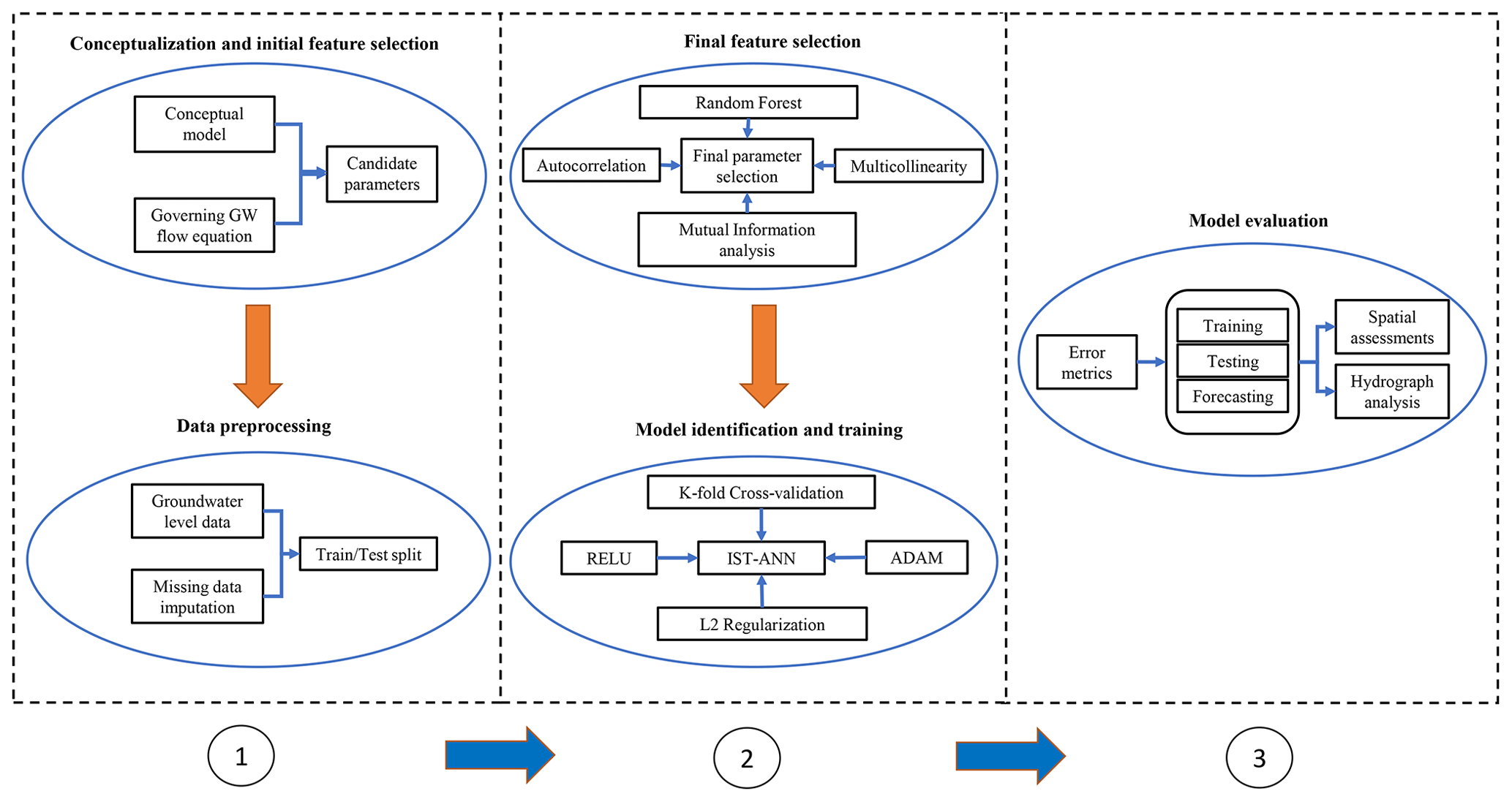
Based on the governing groundwater flow equation, a generic conceptualization of the IST–ANN model can be visualized (see Fig. 1). While the groundwater flow equation provides a good starting point for identifying variables, the selection of certain features (e.g., how many spatiotemporal lags to consider) cannot be directly ascertained. In addition, when aquifer stressors (e.g., pumping) are not directly measured, the selection of an appropriate surrogate cannot be based strictly on physical considerations, especially when more than one surrogate can be used to model the phenomenon of interest. Therefore, as a first step, it is best to cast a wide net and create a comprehensive database of potential inputs (directly measured values and suitable surrogates) for constructing ANN models. Statistical considerations and machine-learning-based parameter selection criteria have been proposed for dimensionality reduction and selection of inputs (Wei et al., 2015; Bi, 2012; Kursa et al., 2010; Kleijnen and Helton, 1999). These approaches can be used to modify and refine physics-inspired specifications of ANN architectures in practical modeling applications.
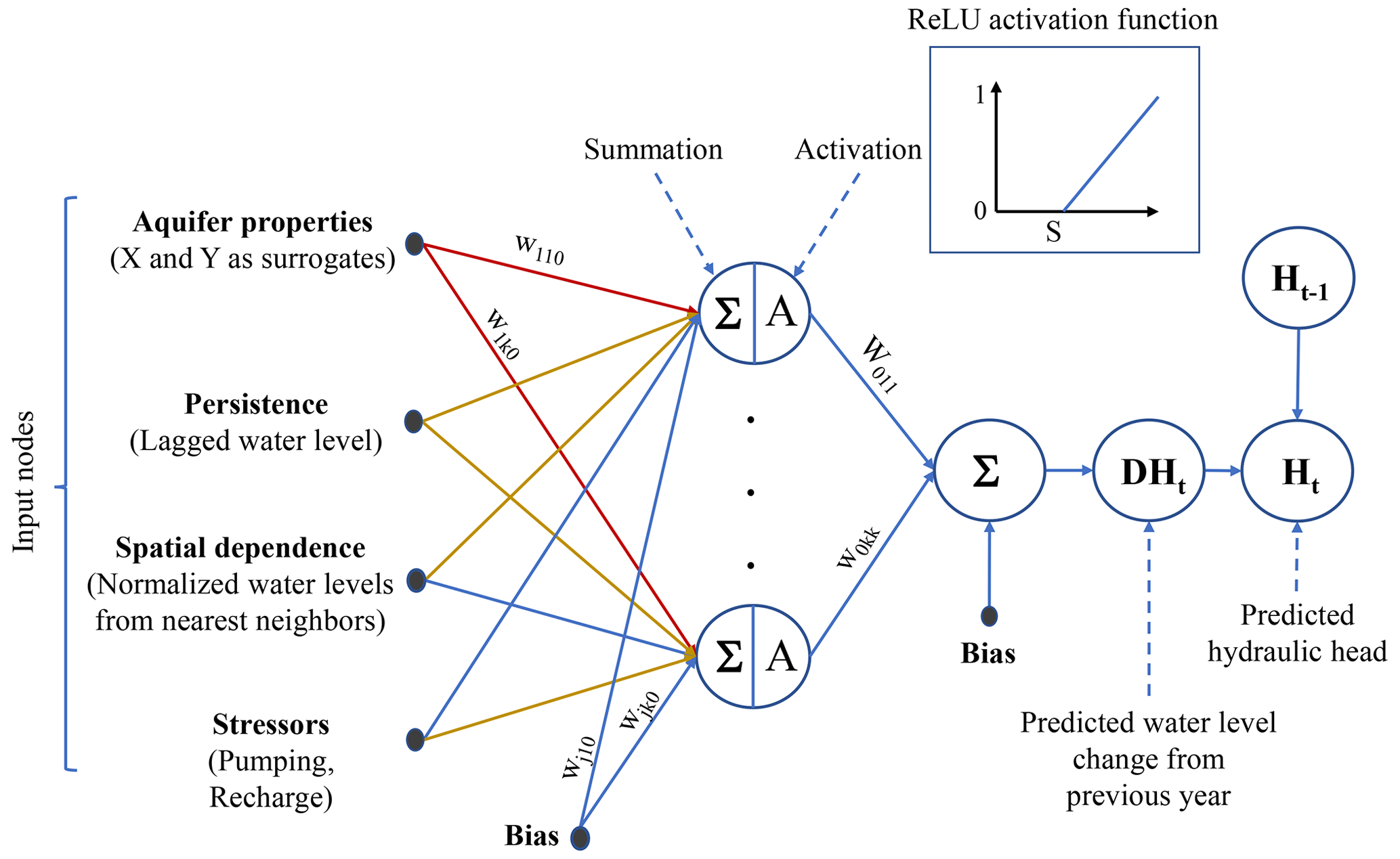
Figure 1A schematic of the IST–ANN model architecture. ReLU denotes the rectified linear unit and Wijk is the weight between ith input and jth hidden neuron within the kth hidden layer.
2.3 Data preprocessing to refine candidate input parameters
Highly correlated input variables share a large amount of common information and, therefore, hamper the learning ability of ANNs (Ahire, 2018). Correlated inputs arise when more than one surrogate can be identified to represent a physical process in a regional-scale ANN. Similarly, lagged variables may also be strongly correlated when the underlying physical processes controlling these variables exhibit persistence. Input multicollinearity can be used as a criterion for the elimination of certain inputs. The mutual information (MI) is an entropy-based metric that measures the amount of information that one random variable has about the other (Bennasar et al., 2015; Vergara and Estévez, 2014). MI can be used to not only rank variables according to their importance but also to select among competing surrogates to represent a process (i.e., variables likely to cause multicollinearity issues). MI can be calculated using Eq. (4), where p denotes the probability density and xi and xj are two (competing) model inputs.
Random forests (RFs; Breiman, 2001) are another machine learning technique that can be used to ascertain variable importance. It has been widely used in several studies as a preprocessing step for identifying suitable input variables (Grömping, 2009; Siroky, 2009; Strobl et al., 2008, 2007). Briefly, RF algorithms construct several decision trees by (1) using a random set of observations and (2) a random subset of candidate variables. The observations not used to build the decision tree are referred to as the out-of-the-bag (OOB) samples. The accuracy of a RF model is proportional to its ability to correctly predict OOB samples (as measured using mean square OOB error, referred to here as OOBMSE). If a candidate input variable (Xj) has no influence on the output, then a random permutation of Xj in OOB samples does not alter the OOB mean square error (OOBMSE) appreciably (i.e., permuted OOBMSE ∼ unpermuted OOBMSE). Variables that have the highest influence cause the greatest increase in the MSE upon permutation. This concept is used to compute the average change in OOB errors associated with each input variable (Xj) of interest over all trees in the forest and to rank inputs according to their importance (Ishwaran et al., 2008).
Variable selection approaches are nonunique, and different approaches can point to different inputs. As such, the use of both MI- and RF-based methods is recommended and adopted in this study. A variable is clearly important if it ranks highly in both techniques and has a well-defined physical meaning. A combination of statistical and physical considerations, theoretical underpinnings, and alternative model conceptualizations can be used to deal with those variables that rank highly under some techniques but not in others.
2.4 IST–ANN model specification
The number of hidden layers plays a key role in defining the architecture of ANNs, and therefore, its specification is an important factor in building these models. In the spirit of model parsimony, a single hidden layer ANN was selected to model regional-scale space–time predictions, as the interpretation of this architecture is straightforward and sufficient for providing universal approximation capabilities (Hornik et al., 1989). The selection of the activation function, which transforms the weighted sum of the inputs entering the hidden node into an output node, is another important decision when configuring ANNs. The rectified linear unit (ReLU) is a nonsaturated activation function, which assumes a value of zero when the weighted summation at the hidden node is less than zero and is equal to the weighted summation otherwise (). ReLU was adopted here (see Fig. 1) as it is known to provide faster convergence with gradient-descent algorithms than conventional saturating activation functions, such as sigmoid and tanh, that have been used in previous groundwater applications of ANNs (Djurovic et al., 2015; Tao et al., 2015; Uddameri, 2007; Nayak et al., 2006).
Overfitting is a major concern in ANN modeling and occurs when the model memorizes the training data set but has poor generalizability (Uddameri, 2007). As overfitting is caused due to the presence of many hidden nodes (some which only learn the noise in the data), the L2 regularization term was added to the objective function to keep the number of hidden nodes to a minimum. As can be seen from Eq. (5), the regularization term increases the objective function when more nodes are added to minimize the mean square error (MSE).
The weighting factor, λ, in Eq. (5) can be treated as a hyperparameter and be estimated as part of the model calibration process.
The adaptive moment or ADAM stochastic gradient descent method (Kingma and Ba, 2014) was used for the minimization of the objective function (see Eq. 5). The ADAM method computes different learning rates for individual parameters which are computed from the bias-corrected first and second moments of the gradients. The method offers several advantages in that the parameter estimates are invariant to the rescaling of the gradients, and the method can effectively deal with sparse gradients and nonstationary objective functions. The ADAM algorithm adds three additional hyperparameters (α,β1, and β2) that control the step size and exponential decay rates. Kingma and Ba (2014) provided good default values for these hyperparameters for use with machine learning optimization problems and were noted to be adequate in this study.
A K-fold cross-validation (K=5) approach was adapted here to further minimize any overfitting concerns. K-fold cross-validation involves randomly splitting the training data set into K equal folds, training a model over (K−1) folds, and testing its adequacy for making predictions using the unused (Kth) subset (i.e., validation fold). The procedure repeats K times, and at each time, a unique fold is treated as a validation subset. The final skill (fitness) score is computed by averaging the errors over all K rounds. The training algorithm was also run in the minibatch mode, where the parameters are updated over a few randomly selected samples rather than the whole data set, as this approach is known to reduce variance in parameter updates and lead to stable convergence (LeCun et al., 2012).
3.1 Study area
The Ogallala Aquifer underlying the High Plains Underground Water Conservation District (HPWD) no. 1 was selected to illustrate the development of the proposed IST–ANN model (see Fig. 2a). The study area is a semiarid region with cool winters and hot summers and spans over 30 691 km2. The topography of the region is characterized by rolling plains, and land surface elevations range from 1353 m in northwestern (NW) part to 810 m in southeastern (SE) portions of the study area (Gutentag et al., 1984). The average annual precipitation is around 480 mm, of which 80 % occurs from April to September (PRISM Climate Group, 2019), during which time most agricultural crops are grown. However, annual precipitation exhibits high temporal variability and decreases when moving westward. The average maximum daily temperature varies between 21.6 and 24.4 ∘C, with cooler temperatures noticed in the northern portions of the study area. However, summer temperatures over 37 ∘C can be experienced over the entire study area. Seasonal precipitation is often insufficient to meet crop water demands, which are exacerbated by high temperatures during critical growth phases. Groundwater from the underlying Ogallala Aquifer is heavily used for irrigation.
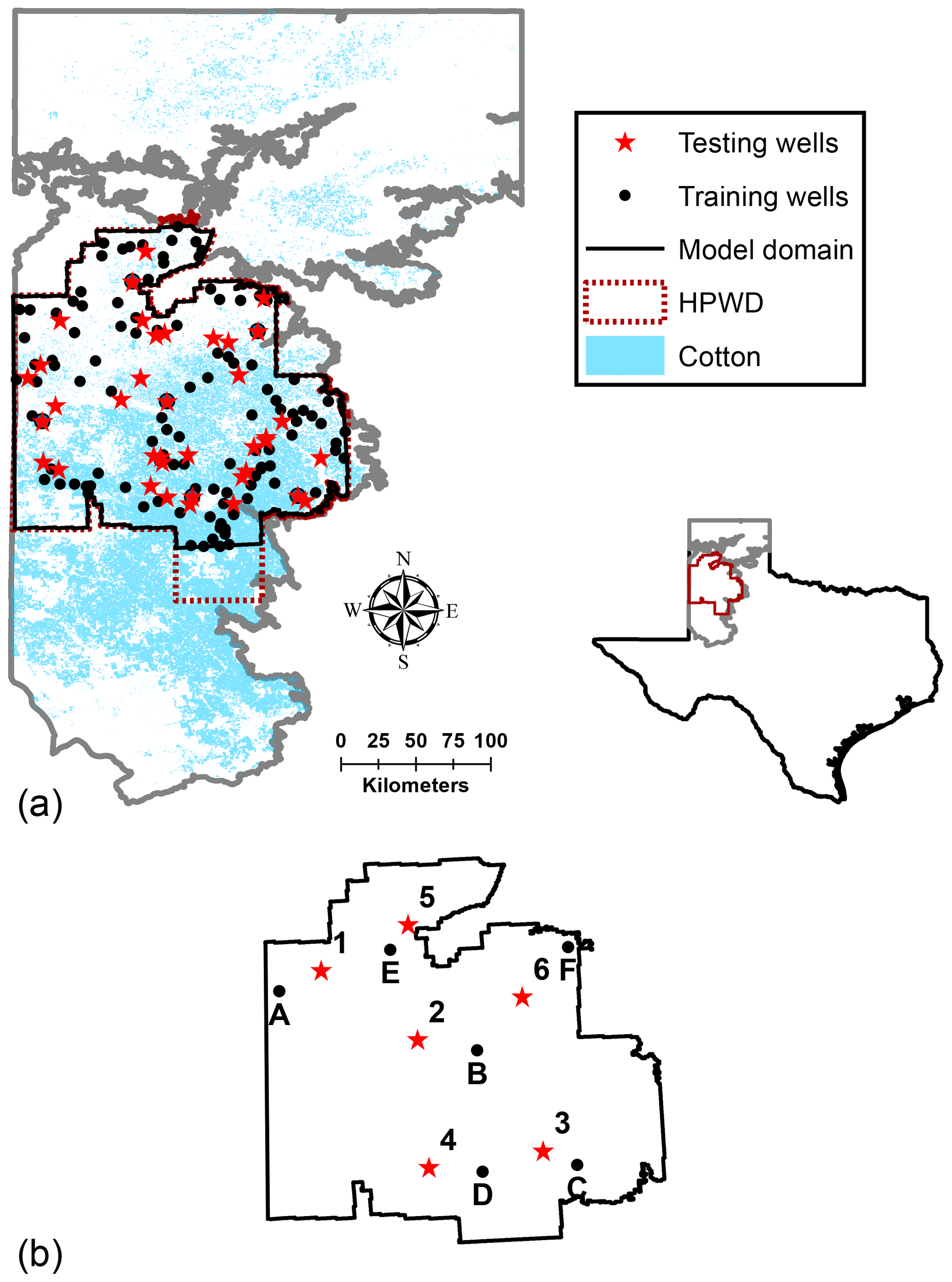
Figure 2(a) Southern High Plains Region of Texas with High Plains Underground Water Conservation District (HPWD) highlighted in black. (b) Wells within HPWD selected to illustrate the temporal variability.
The study area is a groundwater-dependent agricultural economy (Uddameri and Reible, 2018) and accounts for over 20 % of the nation's cotton production (USDA-NASS, 2012). Overexploitation of the aquifer has led to severe water table declines in the region (Scanlon et al., 2012). The food, fiber, and livestock produced in the region are exported across the world, and therefore, the depletion of groundwater in this agriculturally intensive region is not only important for sustaining the local economy but its decline also has severe consequences pertaining to global food security (Marston et al., 2015). The HPWD was created with the mission of conserving and protecting groundwater resources, while ensuring its availability and use for the economic development of the region. As part of its mission, the HPWD has conducted annual groundwater level monitoring campaigns since its creation in 1951. Water levels are collected in the winter, between December and March, as groundwater production during this period is low, and wells exhibit recovery from the summer (irrigation) production back to near-static conditions. The data from this sustained long-term monitoring effort were exploited to develop the IST–ANN model in this study.
3.2 Data compilation
Groundwater level measurements and well information were compiled from the Texas Water Development Board database (TWDB, 2019). A total of 149 wells (see Fig. 2a), with at least 50 years of annual water level measurements between 1955 and 2015, were selected for this study. A total of 12 wells, shown in Fig. 2b, were also selected to illustrate the temporal variability within the study area. The Kalman filtering approach was used to impute the missing data to create continuous annual groundwater level time series data for the period of 1955–2015 (Herrera and Pinder, 2005). Groundwater level changes were computed on an annual basis. For most wells, there was only one reported water level value each year. An average value of the groundwater level was used as a representative value when more than one measurement was made during the winter months. Following McGuire (2017), water level measurements made during summer and fall, if any, were discarded as they do not represent near-static conditions.
Groundwater levels in unconfined aquifers are often a subdued replica of the topography, especially when the recharge is low (Gleeson et al., 2012). As the elevation of the region slopes in the NW–SE direction, the coordinates (X and Y, measured in the Albers equal area projection) of the well were taken as surrogates for the topography. In addition, the aquifer bottom and other aquifer properties exhibit spatial variability. Therefore, the coordinates (X, Y) also serve as indirect surrogates for hydrogeological variability.
As water tables are deep in the region, recharge to the aquifer is practically negligible (Scanlon et al., 2012). Groundwater discharges to streams and rivers are virtually nonexistent due to the lack of hydraulic connection between surface water bodies and the aquifer within the region (Uddameri et al., 2017). Pumping is the major source of groundwater discharge. Historical groundwater pumping data were not available in the region, and this is acknowledged as being a major problem in developing regional-scale models in many agricultural areas (Russo and Lall, 2017). However, as groundwater production is largely for agricultural purposes, the correlation between climate state (drought) indicators and pumping is noted to be strong (Whittemore et al., 2016) and, therefore, a useful surrogate for representing pumping in the ANN model.
The Standardized Precipitation Evapotranspiration Index (SPEI; Vicente-Serrano et al., 2010), with an accumulation period of three months (SPEI-3), was summed annually (January–December) and used as a surrogate for the total annual pumping. The 3-month SPEI is known to correlate well with agricultural water demands in the Great Plains region to which the study area belongs (Zambreski et al., 2018) and is, as such, adopted here. The SPEI-3 values were computed using monthly precipitation and temperature data obtained from PRISM (PRISM Climate Group, 2019) and making use of the Thornthwaite equation for the potential evapotranspiration (Thornthwaite and Mather, 1957). Preliminary comparisons of PRISM data with those measured at meteorological stations indicated the reasonableness of the gridded data set in providing representative precipitation and temperature data within the study area. This data set provided good regional-scale coverage and, thereby, removed the need to impute missing temporal data at individual weather stations; it also helped minimize errors associated with the regionalization of station-level data.
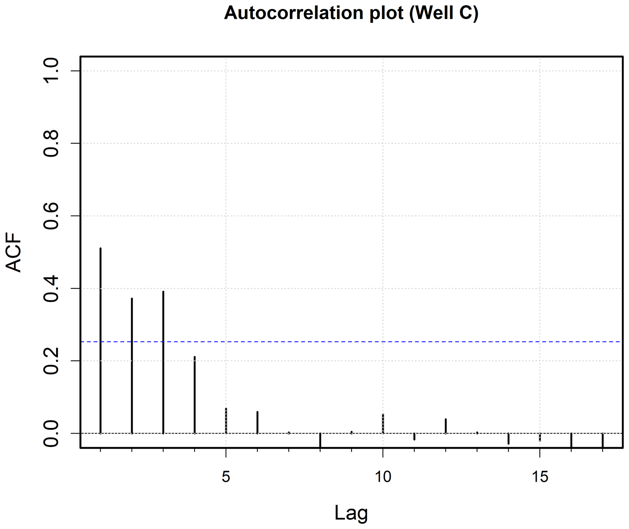
Groundwater levels (GWLs) at each well, GWL(t), in the year (t), i.e., the state variable, along with lagged water levels from 3 previous years labeled as GWL(t−1), GWL(t−2), and GWL(t−3) were compiled into the initial master database. As monitoring wells are randomly scattered in space (Fig. 2a), the neighboring wells were not equidistant. Therefore, an inverse distance normalized lag-1 hydraulic head was used for the neighboring wells (i.e., lag-1 hydraulic head at the neighboring well divided by the distance to the neighboring well) to normalize the effects of nonuniform well spacing. The parameter of the normalized neighboring head was estimated for the four nearest neighboring wells and labeled as , , , and , and the values were also compiled into the master database. SPEI values (a surrogate for water demands and pumping) for the current year, SPEI(t), and the previous 2 years – SPEI(t−1) and SPEI(t−2) – were also added to the database. As the focus was on modeling annual water level time series, three temporal lags and four nearest neighbors were deemed sufficient based on autocorrelation analysis. Higher order lags were noted to have very low () autocorrelation (see Fig. A1 in Appendix A for a representative example). The initial feature (master) database had 116 220 records (149 wells × 60 years × [12 features + 1 state variable]).
3.3 Training, validation, testing, and forecasting data sets
The 149 monitoring wells were randomly split into 111 training wells (75 %) and 38 (25 %) testing wells (see Fig. 2a). The water levels observed in the year 1955 was used as the initial condition. The time period 1956–2015 was split into training and testing (1956–2008) and forecasting (2009–2015) time periods. As shown in Fig. 2a, water levels for the period 1956–2008 at the 111 training wells were used to obtain the connection weights and values for hyperparameters (i.e., the minimum number of hidden nodes, optimal objective function weighting factor, λ, and learning rate). The water level time series data from 1956 to 2008 at the 38 testing wells were used to independently evaluate the prediction abilities of the model (testing error). The water level time series from 2009 to 2015 at all 149 wells were also used to evaluate the forecasting abilities of the models.
Kling et al. (2012)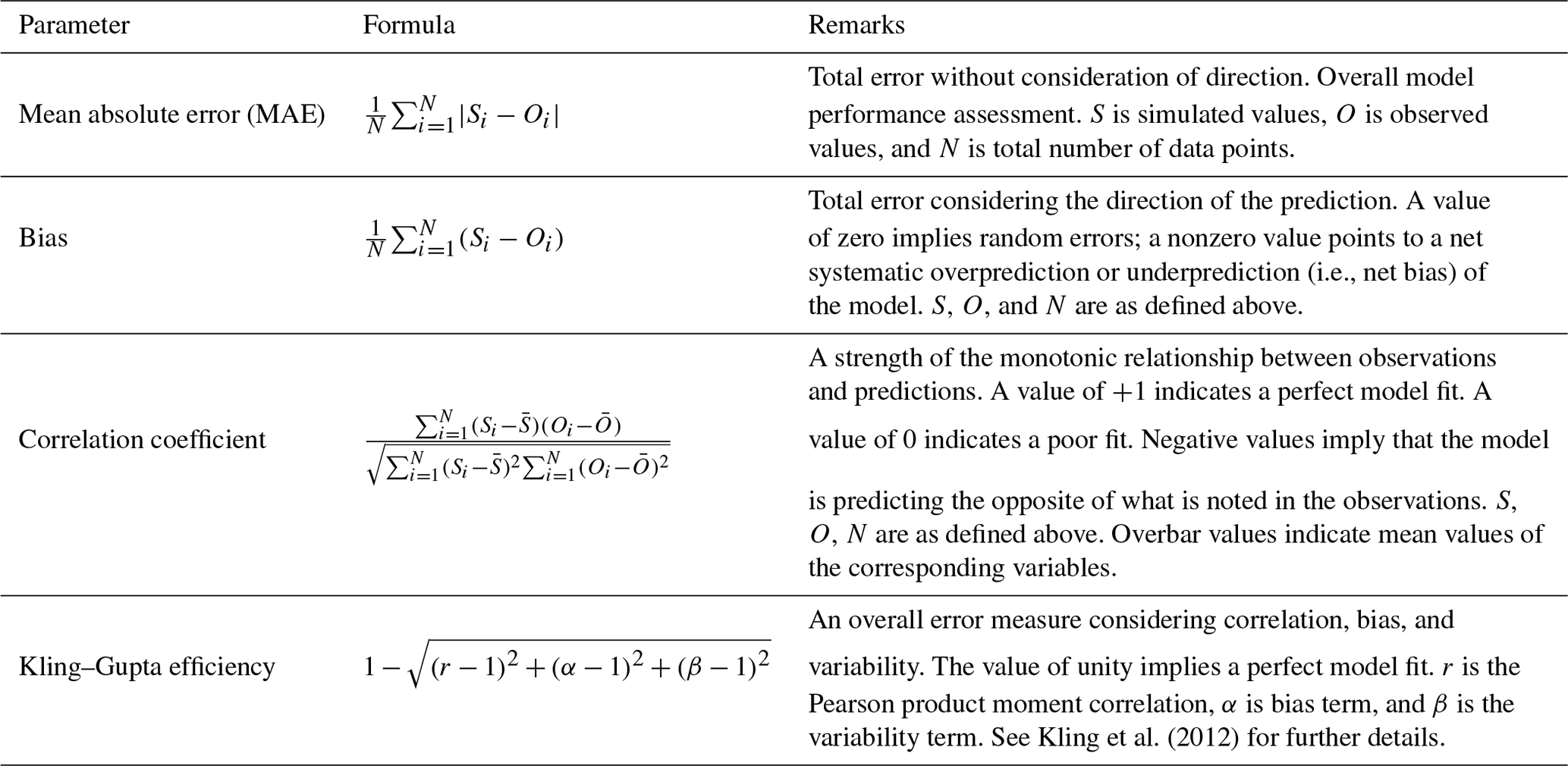
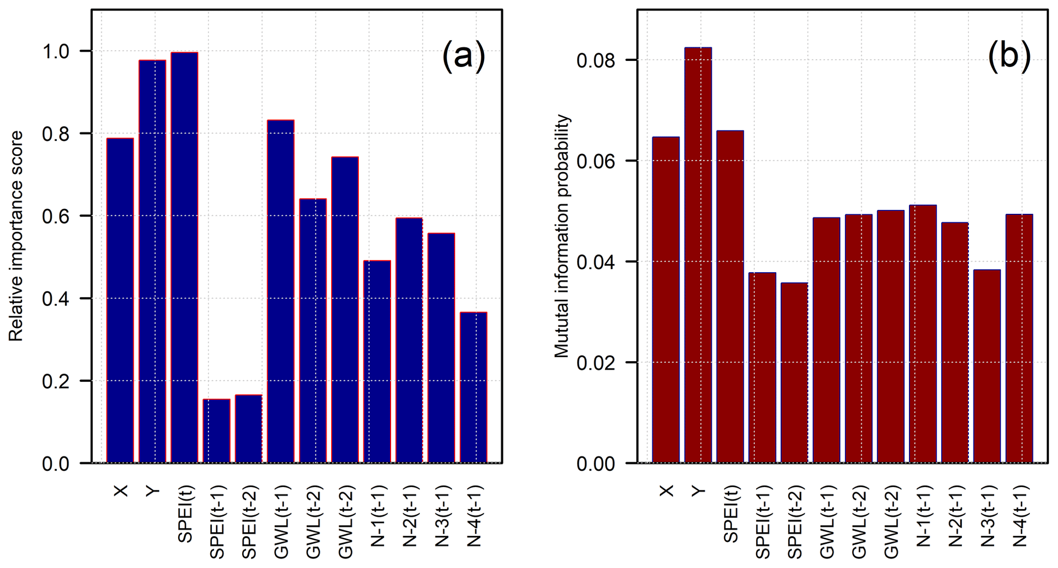
Figure 3Parameter relative importance analysis for different inputs. (a) Importance based on random forest method. (b) Importance based on mutual information method. SPEI(t−k) and GWL(t−k), are the lag-k of standardized precipitation-evapotranspiration index (SPEI) and groundwater level (GWL), respectively. , are the lag-1 of first, second, third, and fourth nearest wells (N).
The one-step-ahead forecasting approach was the primary focus of this study. The training, testing, and forecasting abilities were therefore evaluated in this manner. In other words, forecasts were made for time step (t) using observed data from the previous (t−1) time step. However, the model can also be used to make multistep-ahead predictions using a recursive approach. The performance of the models was evaluated using a suite of methods which included visual observations of well hydrographs, computation of individual well level performance measures, spatial mapping of error metrics, and comparison of observed and simulated hydraulic heads at various time periods. In particular, the mean absolute error (mean nondirectional error), bias (mean directional error), and correlation coefficient were used to quantify the total error, systematic bias, and the strength of the relationship between observed and modeled values. In addition, the Kling–Gupta efficiency (KGE) metric (Kling et al., 2012) was used to evaluate the overall predictive performance considering correlation, bias, and variability. These measures are summarized in Table 1.
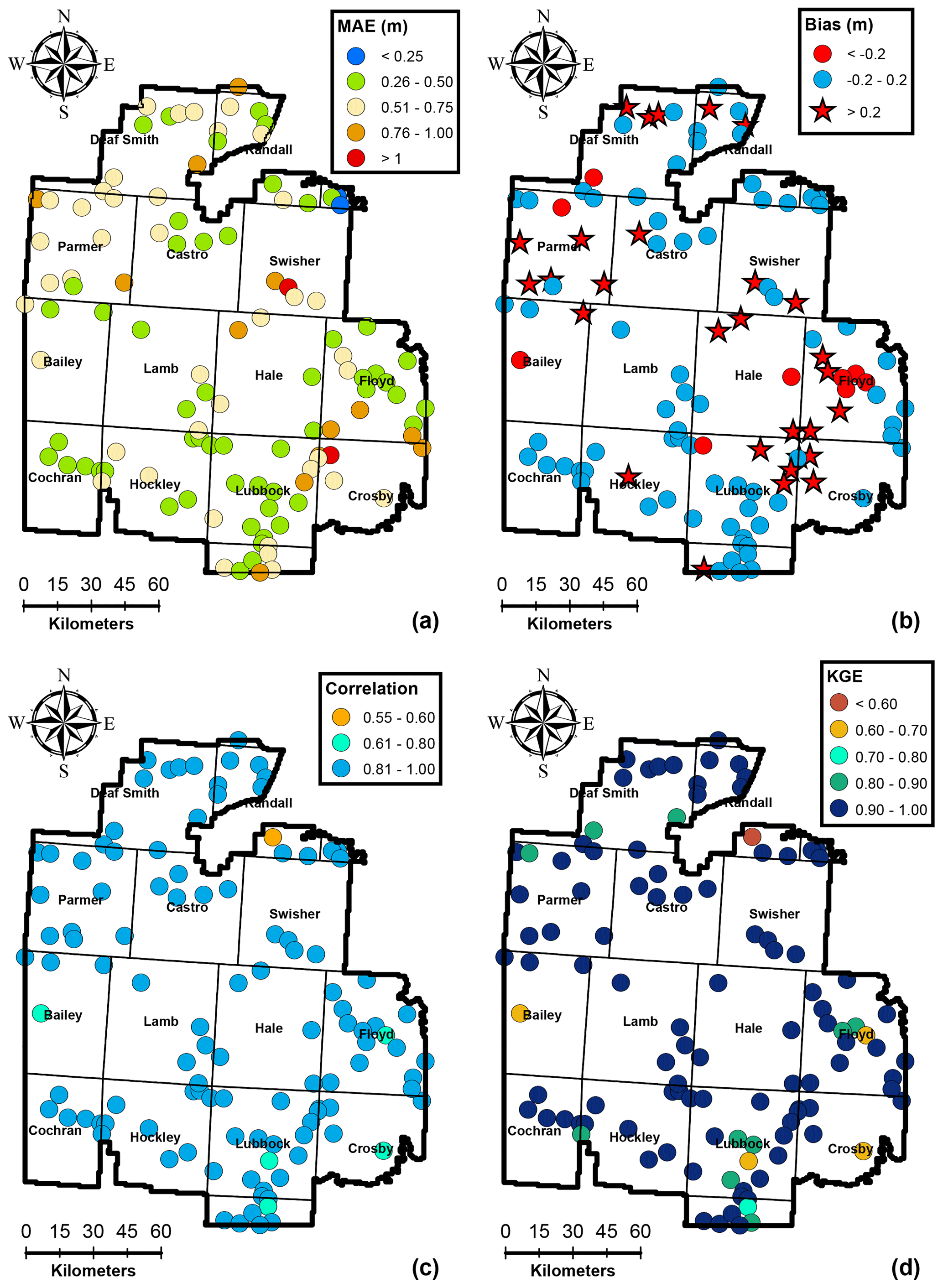
Figure 4Spatial variability of performance measures at 119 training wells for the calibration period 1956–2008.
The IST–ANN modeling was carried out using the Keras open source neural network library (Chollet et al., 2015) with the TensorFlow (Abadi et al., 2016) computational engine in the back end in Python version 3.7.3. In addition, libraries for performing RF-based feature selection (Strobl et al., 2007), mutual information calculations (Meyer, 2014), and computation of model performance measures (Zambrano-Bigiarini, 2014) were carried out by developing custom scripts in the R programming environment and have been made publicly available (Ghaseminejad and Uddameri, 2020). The overall modeling procedure is also illustrated in Fig. A2 in Appendix A.
4.1 Input selection
The mutual information (MI) criterion and the RF-based variable importance metric (relative importance score) along with physical considerations were used to reduce the features (inputs) of the IST–ANN model. Figure 3 indicates that the coordinates (X and Y) were relatively important variables with both selection criteria and, as such, were retained in the final model. The X and Y coordinates were used as surrogates to model the observed variability in the model domain (Gutentag et al., 1984), and as such, their relative importance was to be expected. The Y coordinate was seen to be more important than the X due to a greater variability along the north–south (N–S) axis – more so than the east–west (E–W) axis. There is a considerable climate gradient along the N–S axis (cooler in the north and warmer in the south) which controls the crops grown and, therefore, affects the amount of groundwater extraction more so than the topographical gradient found in the E–W direction. Also, the saturated aquifer thickness exhibits a general N–S variability (McGuire, 2017), and this, in turn, affects the transmissivity of the aquifer within the study area.
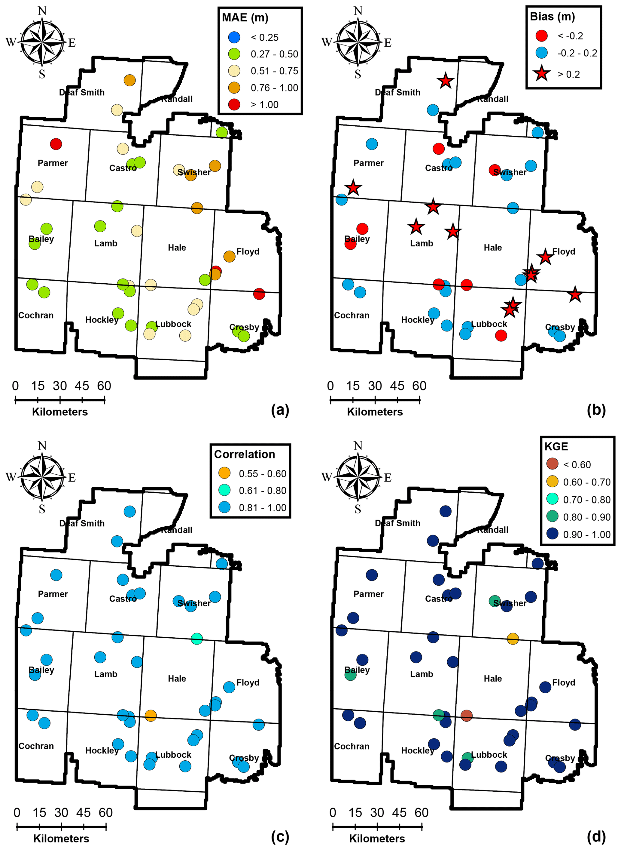
Figure 6Model performance metrics for the testing data set (38 wells) for the period of 1956–2008.
Figure 3 also indicates that lags of SPEI have relatively low importance compared to SPEI values in the current year. This result is again to be expected, as water levels are most affected by groundwater pumping in the immediate past, as limited (or no) production during the winter months allows the water table to recover prior to being stressed again in the summer months. As such, SPEI in the current year was chosen as a model input, and lagged values of SPEI were removed from further consideration in the interests of parsimony.
The lagged water levels at a well represent the memory of the aquifer system with respect to previous stresses (persistence). The lag-1 (previous year) groundwater level was deemed the most important as per the RF model. However, the MI criterion indicated that roughly similar information was shared between the water level in the current year (t) and 3 previous years (t−1, t−2, and t−3). Finite difference groundwater flow simulators, such as MODFLOW (Harbaugh, 2005), often produce excellent results by considering only lag-1 water levels (arising from first-order differencing of the temporal derivatives). Also, as water tables are noted to recover during winters, the lag-1 water level should incorporate the effects of the previous stresses on the aquifer. Therefore, only the lag-1 water level was retained as a model input. In a similar vein, the normalized water levels from four nearest neighbors were retained, based on MI criterion, and are akin to the central differencing schemes often employed to represent spatial derivatives in finite-difference groundwater flow simulators (spatial variability terms). The final IST–ANN model is therefore comprised of eight inputs (X, Y, SPEI(t), GWL(t−1), , , , and in addition to the bias terms.
4.2 Training of ANN models
The performance of the IST–ANN model was a function of the regularization weight, the number of hidden nodes, and the initial learning rate (see Fig. A3 in the appendix). Setting the learning rate to = 0.01, λ=0.005 and the number of hidden nodes to = 12 yielded the lowest mean absolute error over the cross-validation. The low value of regularization weight indicates that overfitting was not of concern here. The 12 hidden nodes are well within the recommended range of (2–17) hidden nodes for an eight input ANN (Maier and Dandy, 2001), and as such, the final architecture was deemed reasonable for the purposes of the study.
The stochastic gradient descent calibration procedure of the IST–ANN model resulted in excellent results across the study area. The mean absolute prediction error was generally below 0.75 m, except at a few wells which had many significant local influences. The calibration model exhibited low bias, and predictions were generally between ±0.2 m for over 67 % of all training wells. In general, the model had exhibited a greater propensity for overestimating the hydraulic heads (∼26 % of the wells) than underestimating the head (∼8 % of training wells). This overestimation is seen along the NW–SE direction within the study area (see Fig. 4b), which represent areas of intensive irrigated agricultural activities. However, the maximum net bias was 0.5 m, and as such, the calibrated predictions are not too far off from the observed values. In general, an overestimation of hydraulic heads implies an underestimation of the groundwater depletion and points to the limitation of using SPEI as a surrogate for groundwater pumping. While SPEI provides a general trend of the climate state, irrigation also depends upon the timing of the rainfall events and days with high temperatures. Substantial irrigation may be necessary, even during normal and wet years, if the rainfall events do not coincide with critical plant growth stages or if the region experiences higher temperatures during rapid plant growth stages which considerably increase the water demand (Uddameri et al., 2017).
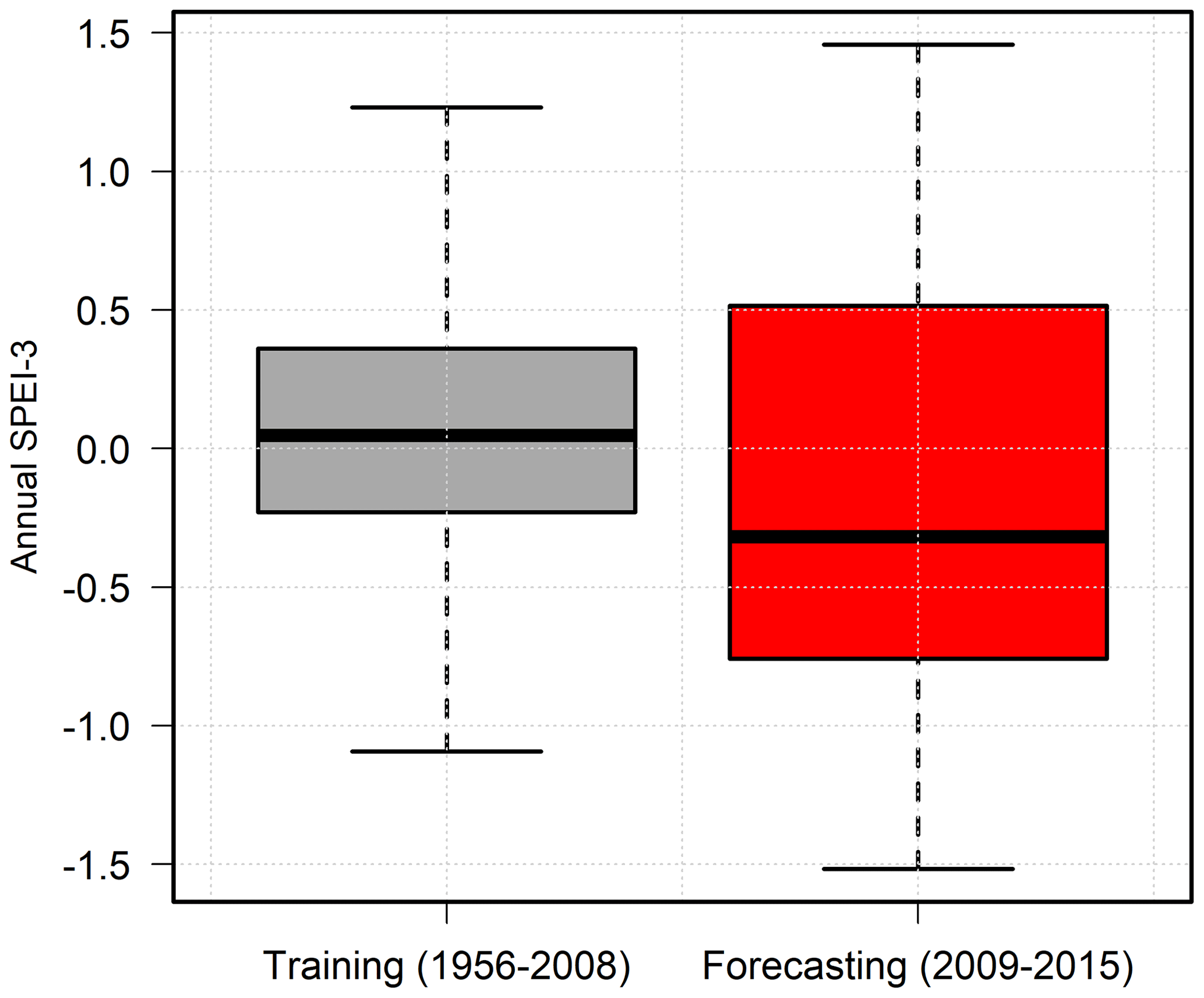
Figure 8Variability in the hydrometeorological conditions during the training and forecasting periods. SPEI-3 denotes the 3-month accumulation standardized precipitation–evapotranspiration index.
The correlation coefficient was >0.8 for 95 % of the training wells, and the overall KGE was greater than 0.8 for 94 % of the calibration wells, indicating the model was able to capture the overall trends in the data, and model predictions were generally not affected by bias and variability as when measured using KGE. Lower KGE values generally corresponded to areas with high localized groundwater production, e.g., in Bailey county where the city of Lubbock (population of ∼ 250 000 and the largest city in the region) has a well field and in Crosby, Floyd, and Lubbock counties where municipal pumping well fields for smaller cities (population of <25 000) exist. While urban water demands are influenced by meteorological conditions incorporated within SPEI (Adamowski et al., 2013), they are also influenced by other factors such as conservation programs (e.g., lawn water restrictions) and cost. Municipal water demands were not included in the present modeling study, as urban areas represent less than 2 % of the study area. However, the results indicate that efforts to capture municipal water demands may locally improve model calibrations. All in all, the calibration of the IST–ANN model can be deemed suitable for regional-scale applications based on the spatial evaluation of time-aggregated performance metrics shown in Fig. 4.
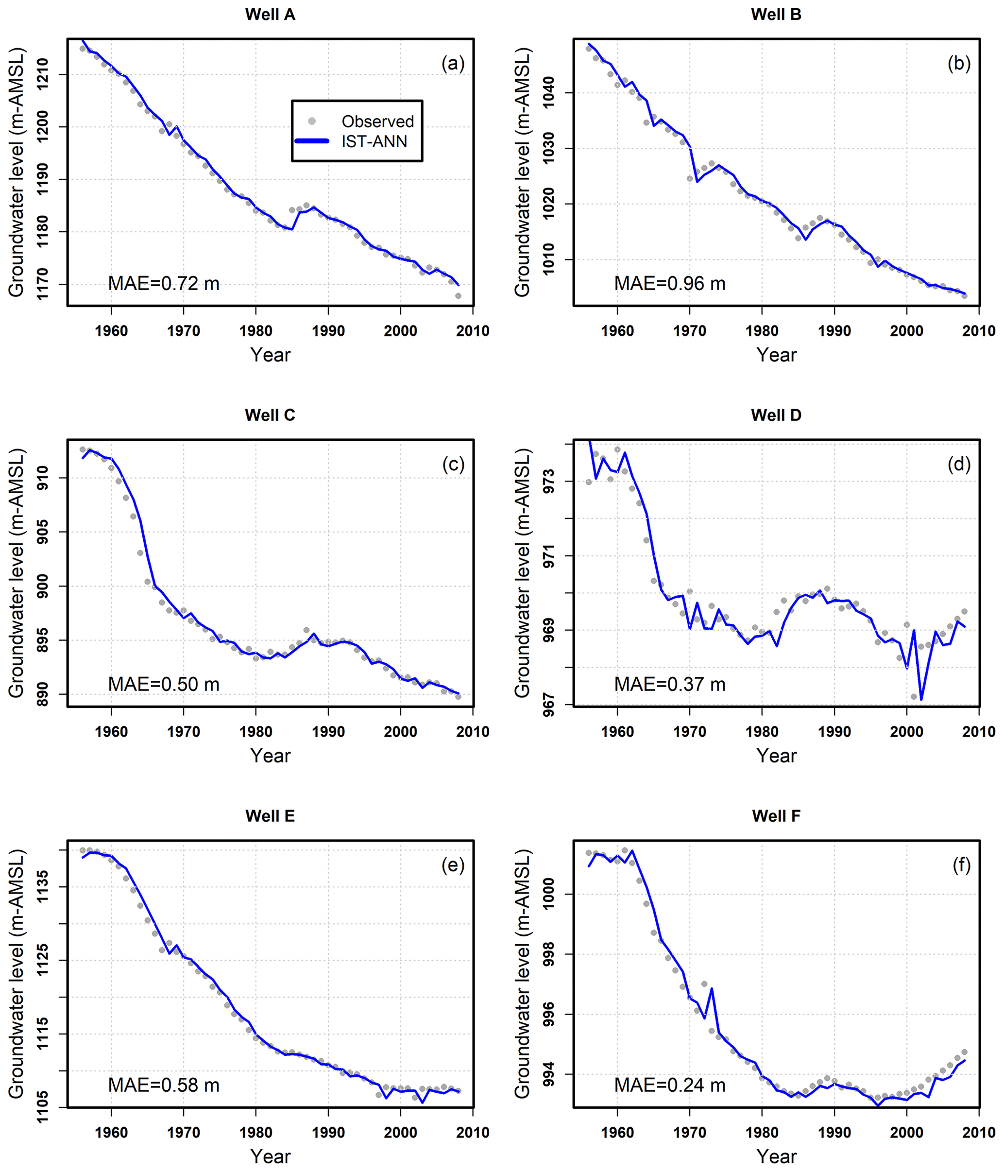
Figure 5 presents representative observed and modeled well hydrographs at selected calibration wells (see Fig. 2b). The selection of these representative wells was done to visualize temporal water level prediction patterns across the region, especially at those wells that had relatively higher mean absolute errors (MAEs). Figure 5 indicates that the IST–ANN model is capable of capturing both the long-term declining trends and short-term volatility caused by anomalous weather events that allowed for higher than normal water level recovery. The results from the well hydrographs, in conjunction with the time-aggregated performance metrics, indicate that the IST–ANN could learn both the spatial and temporal patterns in the data by using a relatively small set of input parameters. While obtaining good calibration is a necessary first step, independent testing of the model at wells not used for calibration is critical for gaining confidence in the model and ensuring the model has not simply memorized the training data set (i.e., overfitting concerns).
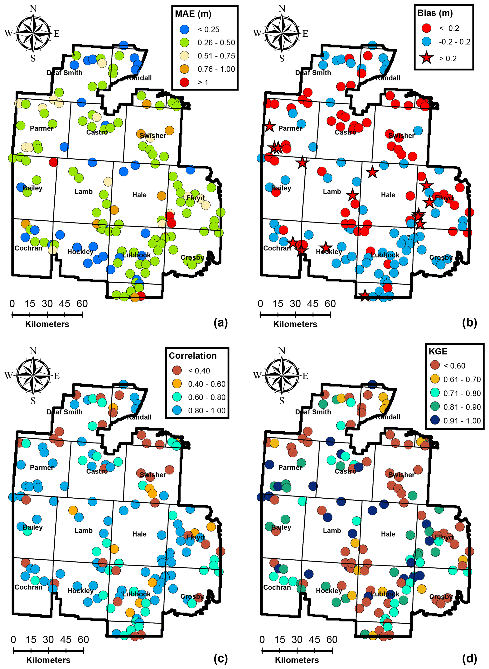
Figure 9Time-aggregated performance metrics for the validation period (2009–2015) for one-step-ahead forecasting at 149 monitoring wells.
4.3 Independent testing of IST–ANN model
Independent testing of the model performance was carried out at 38 wells that were not used for calibration. The time-aggregated performance metrics depicted in Fig. 6 indicate that the model was able to predict groundwater levels at these testing wells with a high degree of accuracy. The mean absolute error for testing wells was less than 0.75 m for 77 % of the wells and less than 1.0 m at 93 % of the wells. The maximum mean absolute error was 1.22 m for the testing data set, which compares favorably with the maximum mean absolute error of 1.14 m for the training data set. The net bias depicted in Fig. 6b shows similar trends to the training data set, with a general overestimation of the hydraulic heads along the NW–SE direction. The maximum net bias was 0.52 m in the testing data set, which is, again, similar to that observed in the training data set (0.50 m). The correlation coefficient and KGE were greater than 0.8 at over 95 % of the testing wells. These results indicate that the calibrated IST–ANN models were able to predict the overall observed behavior in independent wells during the 1956–2008 calibration period. These results confirm that overfitting was not an issue and highlight the ability of the regularization approach to keep the number of hidden nodes to a minimum and help the IST–ANN model focus on its generalization abilities.
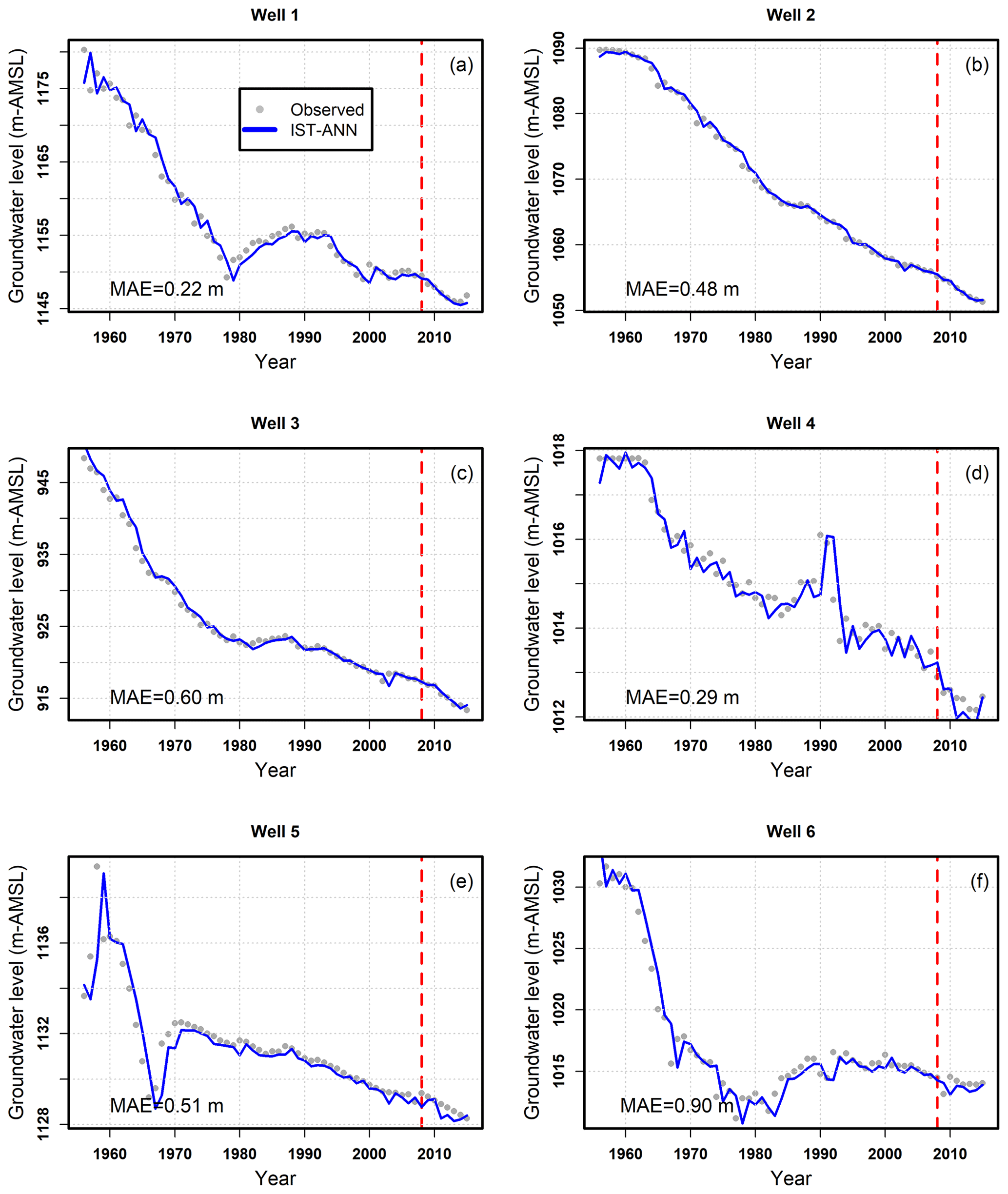
In addition to time-aggregated performance metrics, the ability of the IST–ANN model to capture temporal trends at individual wells was also assessed. Figure 7 depicts the well hydrographs at six representative wells having different mean absolute errors and being scattered across the study area. The results again indicate that the IST–ANN model is able to adequately capture the observed long-term trends in the data. Short-term volatility is pronounced in some wells (see Fig. 7a, d–f), which the IST–ANN model captures well. These results indicate that the IST–ANN not only performs well over a suite of time-aggregated metrics but is also able to capture nuances of water table dynamics noted across the study area. The independent testing of the model adds confidence to the model predictions and confirms the generalization capabilities of the IST–ANN modeling approach.
4.4 Evaluation of forecasting capabilities of the IST–ANN model under extreme climate conditions
While the IST–ANN model was seen to perform well on historical data sets (1956–2008), the performance of the model in forecasting recent water levels is of interest. The period of 2009–2015 was used to assess the forecasting abilities of the model. The forecasting time period represents a time capsule of extreme climate variability as it was characterized by one of the worst droughts seen in the area, including the worst single year of drought in the recorded history of Texas (year 2011) and one of the wettest years (year 2015) recorded in the region. As shown in Fig. 8, the model had to forecast across a range of hydrometeorological conditions that were not represented during the calibration process. As such, the forecasting time period is largely a measure of the extrapolation capabilities of the model.
From a theoretical standpoint, ANNs are not designed to perform extrapolations outside their calibration range (Principe et al., 2000). However, from an application perspective, climate variability is becoming more pervasive and extreme (Thornton et al., 2014; Gutzler and Robbins, 2011). In all likelihood, groundwater models have to be used to make forecasts under hydroclimatic conditions that are very different from those observed during their calibration. Therefore, the ability of data-driven models (which invariably have to be calibrated using long-term historical data) to make forecasts under different hydrometeorological conditions serves as an important check regarding their suitability in practical groundwater management applications.
Model forecasts for the years 2009–2015 were developed at all 149 wells as data from this period were not used for calibration purposes. Figure 9 depicts the performance metrics of the IST–ANN model over the forecasting time period. The mean absolute error (MAE) was less than 0.75 m at 92 % of the wells and less than 1.0 m at 98 % of the wells. The maximum MAE was 1.24 m, which is comparable to that observed during the testing phase (1.22 m). However, the net bias was within ±0.2 m at 48 % of the wells, compared to 53 % in the testing phase. In particular, the maximum observed overprediction (1.04 m) and underprediction (−0.97 m) were much higher than those noted in the testing period (0.52 m and −0.43 m). In addition, the model underpredicted at 42 % of the wells and overpredicted at 11 %. The correlation coefficient was higher than 0.8 in over half of the wells and greater than 0.6 in about three-quarters of the monitoring wells. The KGE values were greater than 0.8 in only 35 % wells, but values were greater than −0.41 in 90 % of the wells, indicating that the model forecasts are significantly better than the mean values (Knoben et al., 2019). The well hydrographs in Fig. 7 for the forecasting time period indicate that the IST–ANN model was typically unable to capture the noted variability in the period but was able to discern general trends in well hydrographs. The variability ratio (Kling et al., 2012) for training, testing, and forecasting data sets is depicted in Fig. 10, and it highlights the high degree of variability noted during the forecasting period.
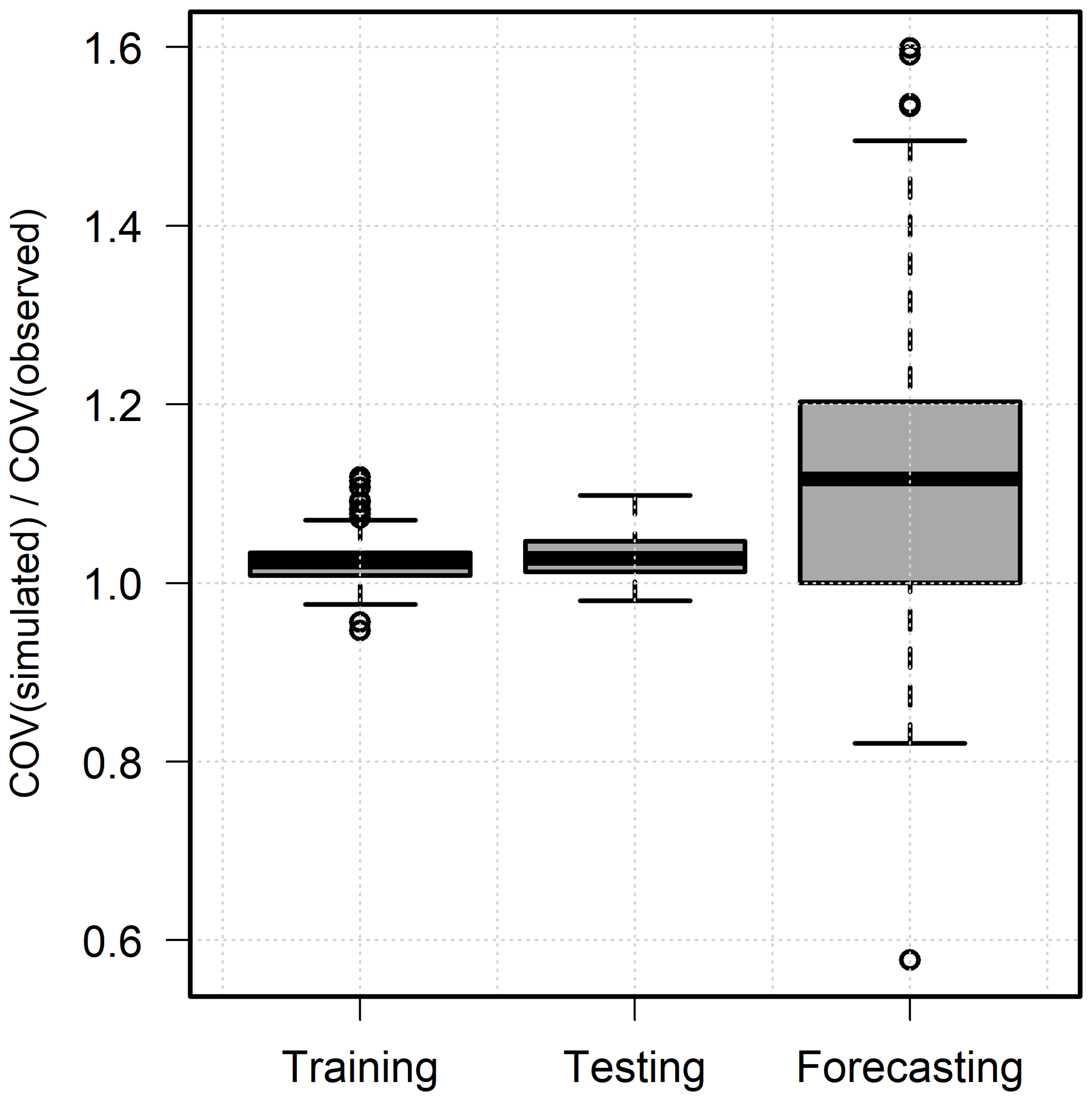
Farmer preferences tend to be heterogeneous within a region (Adhikari et al., 2010), and this heterogeneity was further exacerbated during the severe, prolonged drought experienced during the forecasting period. Some producers in the region chose to increase their groundwater pumping or switched from dryland to irrigated agriculture. Other farmers adopted conservation practices which led to reduced groundwater use. These heterogeneous farmer preferences, and their adaptation to prolonged drought and extreme climate, explain the observed variability in Fig. 10.
There were no variables in the model to capture these preferences of the groundwater users in the region. The spatial variability in SPEI (surrogate for pumping) was considerably small as all of the study area experienced severe drought conditions, and this parameter was insufficient for capturing the observed variability in pumping. The difference in observed and simulated variance played a critical role in reducing the correlation coefficient and KGE metrics during the forecasting period.

Figure 11Water table contour map (left column) and one-step-ahead forecasting errors (right column) shown during (a, b) dry (2011), (c, d) normal (2014), and (e, f) wet (2015) years.
As climatic conditions play a critical role in defining groundwater extractions, spatial variability in forecasting errors was assessed by comparing with observed water levels in 2011 (worst drought year in the recorded history of Texas; mean SPEI-3 ), 2014 (a relatively normal year; mean SPEI-3 ∼0), and 2015 (a wet year; mean SPEI-3 ). The results depicted in Fig. 11 show that the fraction of the study area, where the predicted drawdown error was less than 1 m, was highest under normal climatic conditions and deviated under both dry and wet conditions. However, the deviations were relatively small under wet conditions than those under dry conditions. The absolute error was less than 2 m for 88 % of the study area in 2011 (dry year) but was 92 % and 94 % in normal (2014) and wet (2015) years. This result highlights that, in addition to the volume of the net rainfall (that is captured using SPEI-3), the timing of the rainfall events also plays an important role. Even in relatively wet years, rainfall may not occur during critical crop growth periods and warrant significant levels of irrigation. While SPEI correlates strongly with agricultural conditions, it is not an agricultural drought indicator per se. Agricultural drought indices, especially those using soil moisture measurements, could serve as better surrogates for capturing irrigation dynamics. However, ground truthing soil-moisture-based agriculture drought indicators is often challenging due to the paucity of the data, and these soil moisture indices do not include irrigation water applications (Tsige et al., 2019). Therefore, these indicators may not be full substitutes for the lack of groundwater pumping data.
4.5 Input parameter sensitivity
The relative impact of the input parameters on the output was explored by looking at the connection weights of the IST–ANN model (Olden et al., 2004). The sensitivity of the model output to various input values are depicted in Fig. 12 (also see Appendix B for the relative important index calculation). The predicted groundwater level changes were most sensitive to SPEI, as irrigated agriculture is the primary user of groundwater in the study area. The well coordinates were used as a surrogate to capture the variability in the aquifer properties. The saturated thickness in the study area has a distinct north–south variability (McGuire, 2017). This variability, in turn, affects the aquifer transmissivity, a key hydrogeological parameter that affects hydraulic heads and explains the high sensitivity of the model output to the Y coordinate.
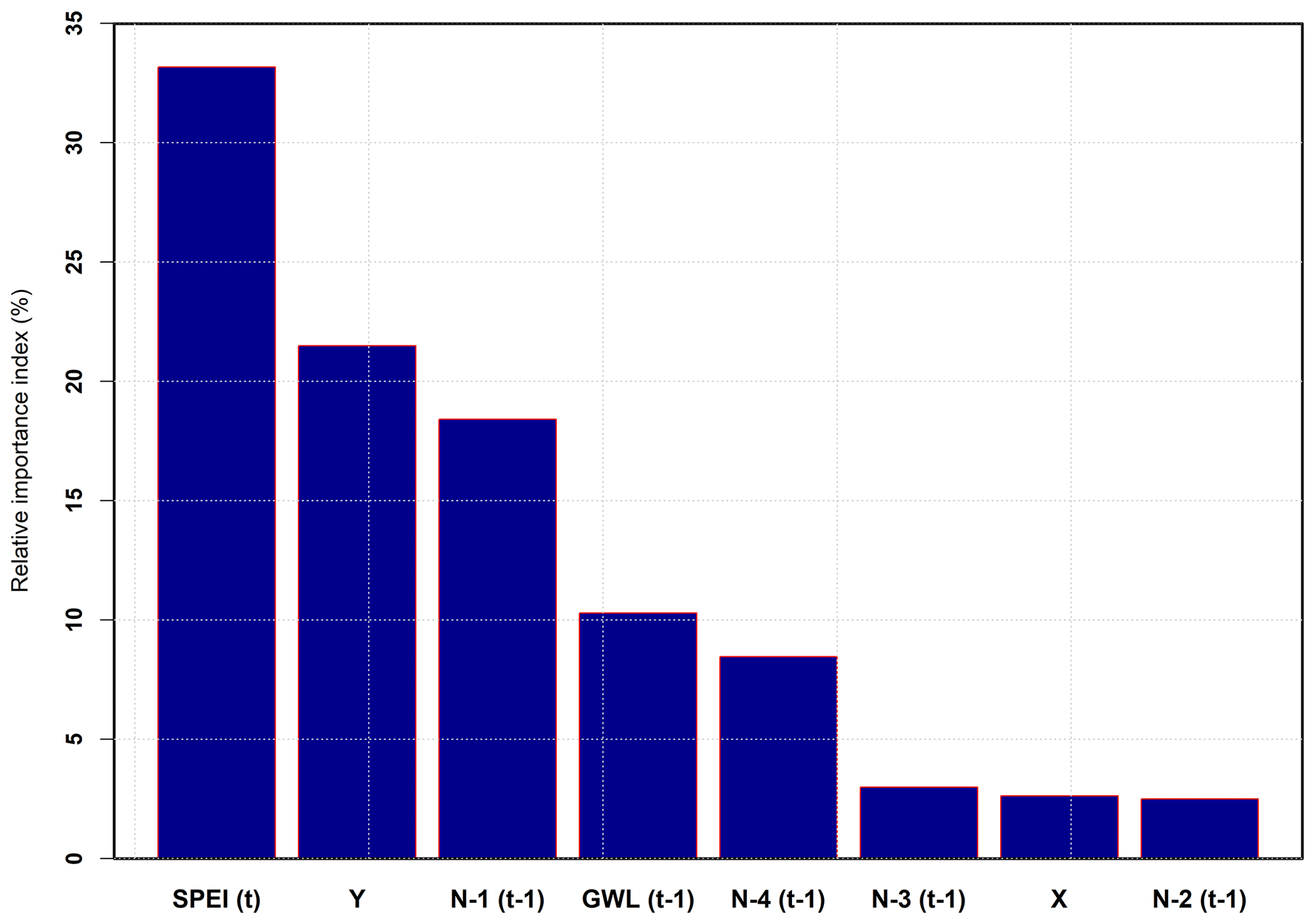
Figure 12Relative importance of model inputs in the prediction of groundwater levels. SPEI(t) and GWL(t−1) are the current year's standardized precipitation–evapotranspiration index and lag-1 of groundwater level, respectively. and are the lag-1 of the first, second, third, and fourth nearest wells. X and Y are Cartesian coordinates.
The sensitivity analysis also suggests that the normalized hydraulic heads at neighboring wells (spatial-dependence terms) affected the model predictions, followed by the lagged groundwater level. The predicted groundwater level at a time (t) and at a given well depends upon how quickly water can flow into the well. Both the groundwater level at the neighboring well and GWL(t−1) are necessary for computing the hydraulic gradient which determines the rate of water movement to a well. The predicted groundwater level was also seen to be somewhat sensitive to the normalized hydraulic head at the fourth nearest well . The fourth nearest well was typically located along the Y axis, and this sensitivity denotes the anisotropic nature of groundwater flow – at least in some portions of the study area (Gutentag et al., 1984).
The primary goal of this study was to evaluate the hypothesis that a parsimonious ANN model can be constructed to model regional-scale aquifer dynamics in space and time. An integrated space–time artificial neural network model (IST–ANN) was specified, drawing inspiration from the governing groundwater flow equation. The lack of available data to directly include pertinent hydrogeological processes is a challenge in practical groundwater modeling studies. Machine-learning-based feature selection algorithms were therefore used to identify a suitable set of inputs to parameterize the model. Recent advances in ANN model calibration, namely regularization, adaptive moment stochastic gradient algorithm, along with five-fold cross-validation were used to minimize model overfitting. A 8–12–1 (no. of inputs–no. of hidden neurons–no. of output) architecture was noted to be optimal for modeling a 30 691 km2 section of the Ogallala Aquifer underlying the High Plains Underground Water Conservation District (HPWD) in the southern High Plains of Texas. Input variables included location parameters (to capture hydrogeological variability), lagged water levels at the well (a measure of persistence), and water levels at the four nearest neighboring wells to capture spatial dependence. Groundwater pumping – a critical stressor – was modeled using the 3-month accumulation standardized precipitation evapotranspiration index (SPEI).
An excellent calibration was obtained using data from the period of 1956–2009 at 119 wells within the study area. The independent testing of the model at 38 wells over the same time period indicated that the IST–ANN model was able to correctly simulate groundwater level dynamics at these independent wells over the 1956–2008 time period, indicating that overfitting was not an issue. The IST–ANN model was then used to forecast water levels at 149 wells (training and testing wells) using another independent data set corresponding to the 2009–2015 time period. This time period was marked by a severe and prolonged drought which ended with a very wet year (2015) in the study area. The hydroclimatic conditions during the forecasting period were largely outside the range of variability noted during the calibration period of 1956–2008. While data-driven models such as ANNs are largely interpolation methods, the changing climate implies that these models will mostly be used in an extrapolation mode as historical hydrometeorological conditions are unlikely to be the same as those for future forecasting time periods. While the IST–ANN model did not extrapolate as well during the forecasting time period, the model was able to capture general trends and provide estimates that were generally better than historical averages.
Model sensitivity analysis was carried out by looking at the connection weights. SPEI (a surrogate) used for pumping was noted to be the most sensitive parameter, indicating the importance of groundwater pumping on aquifer water level predictions. The Y coordinate was the next most sensitive parameter as it sought to capture the heterogeneity of the aquifer parameters. In particular, the N–S variability in the groundwater levels plays an important role in controlling aquifer transmissivity and, therefore, water level predictions. The normalized nearest neighbor(s) – an indicator of spatial dependence – was (were) noted to be more sensitive than the lagged water level at the well (hydrogeological persistence term). Water levels in the nearest neighbor affect the local hydraulic gradients and control the rate of groundwater movement to a well. These results suggest that the developed IST–ANN model exhibits a high fidelity to the hydrogeological principles and conditions within the study area.
The results of the study indicate that parsimonious neural network formulations hold promise for modeling regional-scale groundwater levels in space and time. Simulating groundwater levels in agricultural regions, especially under climate extremes, requires an understanding of how farmers (groundwater users) adapt to drought conditions. Farmers exhibit heterogeneous behavior and choose to increase pumping or adopt conservation measures. Therefore, climate indicators, while pragmatic, may not fully capture the groundwater production preferences of farmers. Better surrogates for capturing this human dimension of groundwater production are critical if data-driven models have to be extrapolated to situations that are not reflective of historical conditions to which they are calibrated.
A1 Autocorrelation analysis
A2 The applied modeling procedure flowchart
A3 Regularization of IST–ANN model
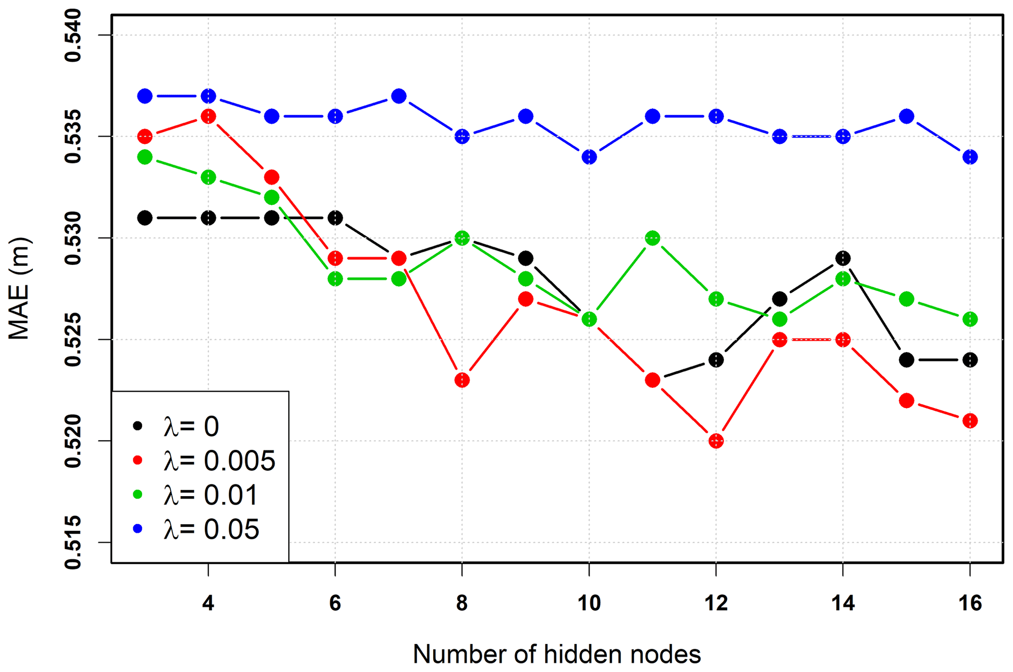
Figure A3The performance of the IST–ANN model for various regularization weights and a number of hidden nodes (learning rate = 0.01).
According to Olden et al. (2004), in a model with M number of inputs (i), one output (k), and one hidden layer containing N nodes (j), the relative importance (RE) corresponding to each input can be computed as follows:
where wij and wjk are input-hidden weights and hidden-output weights, respectively.
The data set and custom scripts (Python and R) developed for this study are available at https://doi.org/10.17605/OSF.IO/5KV6R (Ghaseminejad and Uddameri, 2020).
VU and AG conceptualized the study and developed the methodology. AG visualized the project, developed the model software, and conducted the formal analysis. VU validated the data, acquired the funding, and administered the project. VU wrote the original draft, and both VU and AG contributed to the reviewing and editing of the paper.
The authors declare that they have no known competing financial interests or personal relationships that could have appeared to influence the work reported in this paper.
This article is based upon work that is supported by the “Sustaining Agriculture through Adaptive Management to Preserve the Ogallala Aquifer under a Changing Climate” project (USDA-NIFA; grant no. 2016-68007-25066). We also acknowledge the High Plains Underground Water District and Texas Water Development Board for collecting and providing the data used in this study. We thank the reviewers and the editor for their thoughtful comments and review.
This research has been supported by the National Institute of Food and Agriculture (NIFA) of the U.S. Department of Agriculture (USDA; grant no. 2016-68007-25066).
This paper was edited by Dimitri Solomatine and reviewed by Ashes Banerjee and one anonymous referee.
Abadi, M., Agarwal, A., Barham, P., Brevdo, E., Chen, Z., Citro, C., Corrado, G. S., Davis, A., Dean, J., Devin, M., Ghemawat, S., Goodfellow, I. J., Harp, A., Irving, G., Isard, M., Jia, Y., Józefowicz, R., Kaiser, L., Kudlur, M., Levenberg, J., Mané, D., Monga, R., Moore, S., Murray, D. G., Olah, C., Schuster, M., Shlens, J., Steiner, B., Sutskever, I., Talwar, K., Tucker, P. A., Vanhoucke, V., Vasudevan, V., Viégas, F. B., Vinyals, O., Warden, P., Wattenberg, M., Wicke, M., Yu, Y., and Zheng, X.: TensorFlow: Large-Scale Machine Learning on Heterogeneous Distributed Systems, CoRR, abs/1603.04467, http://arxiv.org/abs/1603.04467, 2016. a
Adamowski, J. and Chan, H. F.: A wavelet neural network conjunction model for groundwater level forecasting, J. Hydrol., 407, 28–40, https://doi.org/10.1016/j.jhydrol.2011.06.013, 2011. a
Adamowski, J., Adamowski, K., and Prokoph, A.: A spectral analysis based methodology to detect climatological influences on daily urban water demand, Math. Geosci., 45, 49–68, 2013. a
Adhikari, S., Belasco, E. J., and Knight, T. O.: Spatial producer heterogeneity in crop insurance product decisions within major corn producing states, Agric. Financ. Rev., 70, 66–78, 2010. a
Ahire, J.: Artificial Neural Networks: the Brain behind AI, Lulu. com, ISBN 1980483671, 9781980483670, 2018. a
Amaranto, A., Munoz-Arriola, F., Solomatine, D., and Corzo, G.: A spatially enhanced data-driven multimodel to improve semiseasonal groundwater forecasts in the High Plains aquifer, USA, Water Resour. Res., 55, 5941–5961, 2019. a
Anderson, M. P., Woessner, W. W., and Hunt, R. J.: Applied groundwater modeling: simulation of flow and advective transport, Academic press, ISBN 978-0-12-058103-0, Academic Press, Cambridge, MA, USA, https://doi.org/10.1016/C2009-0-21563-7, 2015. a
Barnes, S. L.: A technique for maximizing details in numerical weather map analysis, J. Appl. Meteorol., 3, 396–409, 1964. a
Bennasar, M., Hicks, Y., and Setchi, R.: Feature selection using joint mutual information maximisation, Expert Syst. Appl., 42, 8520–8532, 2015. a
Bi, J.: A review of statistical methods for determination of relative importance of correlated predictors and identification of drivers of consumer liking, J. Sens. Stud., 27, 87–101, 2012. a
Breiman, L.: Random forests, Mach. Learn., 45, 5–32, 2001. a
Chollet, F. et al.: Keras, available at: https://keras.io (last access: 20 January 2020), 2015. a
Daliakopoulos, I. N., Coulibaly, P., and Tsanis, I. K.: Groundwater level forecasting using artificial neural networks, J. Hydrol., 309, 229–240, 2005. a
Djurovic, N., Domazet, M., Stricevic, R., Pocuca, V., Spalevic, V., Pivic, R., Gregoric, E., and Domazet, U.: Comparison of Groundwater Level Models Based on Artificial Neural Networks and ANFIS, Sci. World J., 2015, 742138, https://doi.org/10.1155/2015/742138, 2015. a
Farthing, M. W., Kees, C. E., and Miller, C. T.: Mixed finite element methods and higher order temporal approximations for variably saturated groundwater flow, Adv. Water Resour., 26, 373–394, 2003. a
Ghaseminejad, A. and Uddameri, V.: Dataset and codes for Physics-inspired integrated space-time Artificial Neural Networks for regional groundwater flow modeling, Open Science Framework (OSF) data repository, https://doi.org/10.17605/OSF.IO/5KV6R, 2020. a, b
Gleeson, T., Alley, W. M., Allen, D. M., Sophocleous, M. A., Zhou, Y., Taniguchi, M., and VanderSteen, J.: Towards sustainable groundwater use: setting long-term goals, backcasting, and managing adaptively, Groundwater, 50, 19–26, 2012. a
Gómez-Hernández, J. J. and Gorelick, S. M.: Effective groundwater model parameter values: Influence of spatial variability of hydraulic conductivity, leakance, and recharge, Water Resour. Res., 25, 405–419, 1989. a
Grömping, U.: Variable importance assessment in regression: linear regression versus random forest, Am. Stat., 63, 308–319, 2009. a
Gutentag, E. D., Heimes, F. J., Krothe, N. C., Luckey, R. R., and Weeks, J. B.: Geohydrology of the High Plains aquifer in parts of Colorado, Kansas, Nebraska, New Mexico, Oklahoma, South Dakota, Texas, and Wyoming, US Government Printing Office Washington, DC, 1984. a, b, c
Gutzler, D. S. and Robbins, T. O.: Climate variability and projected change in the western United States: regional downscaling and drought statistics, Clim. Dyn., 37, 835–849, 2011. a
Harbaugh, A. W.: MODFLOW-2005, the US Geological Survey modular ground-water model: the ground-water flow process, US Department of the Interior, US Geological Survey Reston, VA, 2005. a, b, c
Herrera, G. S. and Pinder, G. F.: Space-time optimization of groundwater quality sampling networks, Water Resour. Res., 41, W12407, https://doi.org/10.1029/2004WR003626, 2005. a
Hornik, K., Stinchcombe, M., and White, H.: Multilayer feedforward networks are universal approximators, Neural networks, 2, 359–366, 1989. a, b
Isaaks, E. H. and Srivastava, M. R.: Applied geostatistics, 551.72 ISA, Oxford University Press, ISBN 0195050134, 9780195050134, 1989. a
Ishwaran, H., Kogalur, U. B., Blackstone, E. H., Lauer, M. S., and Others: Random survival forests, Ann. Appl. Stat., 2, 841–860, 2008. a
Kingma, D. P. and Ba, J.: Adam: A method for stochastic optimization, arXiv [preprint], arXiv1412.6980, 2014. a, b
Kleijnen, J. P. C. and Helton, J. C.: Statistical analyses of scatterplots to identify important factors in large-scale simulations, 1: Review and comparison of techniques, Reliab. Eng. Syst. Saf., 65, 147–185, 1999. a
Kling, H., Fuchs, M., and Paulin, M.: Runoff conditions in the upper Danube basin under an ensemble of climate change scenarios, J. Hydrol., 424, 264–277, 2012. a, b, c
Knoben, W. J. M., Freer, J. E., and Woods, R. A.: Technical note: Inherent benchmark or not? Comparing Nash–Sutcliffe and Kling–Gupta efficiency scores, Hydrol. Earth Syst. Sci., 23, 4323–4331, https://doi.org/10.5194/hess-23-4323-2019, 2019. a
Kursa, M. B., Jankowski, A., and Rudnicki, W. R.: Boruta – a system for feature selection, Fundam. Informaticae, 101, 271–285, 2010. a
LeCun, Y. A., Bottou, L., Orr, G. B., and Müller, K.-R.: Efficient backprop, in: Neural networks: Tricks of the trade, pp. 9–48, Springer, 2012. a
Liu, D., Li, G., Fu, Q., Li, M., Liu, C., Faiz, M. A., Khan, M. I., Li, T., and Cui, S.: Application of Particle Swarm Optimization and Extreme Learning Machine Forecasting Models for Regional Groundwater Depth Using Nonlinear Prediction Models as Preprocessor, J. Hydrol. Eng., 23, 4018052, 2018. a
Maier, H. R. and Dandy, G. C.: Neural network based modelling of environmental variables: a systematic approach, Math. Comput. Model., 33, 669–682, 2001. a
Marston, L., Konar, M., Cai, X., and Troy, T. J.: Virtual groundwater transfers from overexploited aquifers in the United States, P. Natl. Acad. Sci., 112, 8561–8566, 2015. a
McGuire, V. L.: Water-level and recoverable water in storage changes, High Plains aquifer, predevelopment to 2015 and 2013–15: U.S. Geological Survey Scientific Investigations Report 2017–5040, 14 p., https://doi.org/10.3133/sir20175040, 2017. a, b, c
Meyer, P. E.: infotheo: Information-Theoretic Measures, available at: https://cran.r-project.org/package=infotheo (last access: 2 February 2020), 2014. a
Mickens, R. E.: Advances in the Applications of Nonstandard Finite Diffference Schemes, World Scientific, 2005. a
Mohanty, S., Jha, M. K., Raul, S., Panda, R., and Sudheer, K.: Using artificial neural network approach for simultaneous forecasting of weekly groundwater levels at multiple sites, Water Resour. Manag., 29, 5521–5532, 2015. a
Nayak, P. C., Satyaji Rao, Y. R., and Sudheer, K. P.: Groundwater level forecasting in a shallow aquifer using artificial neural network approach, Water Resour. Manag., 20, 77–90, https://doi.org/10.1007/s11269-006-4007-z, 2006. a, b
Nizar Shamsuddin, M. K., Mohd Kusin, F., Sulaiman, W. N. A., Ramli, M. F., Tajul Baharuddin, M. F., and Adnan, M. S.: Forecasting of Groundwater Level using Artificial Neural Network by incorporating river recharge and river bank infiltration, in: MATEC Web Conf., 103, 04007, https://doi.org/10.1051/matecconf/201710304007, 2017. a
Nourani, V., Mogaddam, A. A., and Nadiri, A. O.: An ANN-based model for spatiotemporal groundwater level forecasting, Hydrol. Process. An Int. J., 22, 5054–5066, 2008. a, b
Nourani, V., Ejlali, R. G., and Alami, M. T.: Spatiotemporal Groundwater Level Forecasting in Coastal Aquifers by Hybrid Artificial Neural Network-Geostatistics Model: A Case Study, Environ. Eng. Sci., 28, 217–228, https://doi.org/10.1089/ees.2010.0174, 2011. a
Obergfell, C., Bakker, M., and Maas, K.: Identification and explanation of a change in the groundwater regime using time series analysis, Groundwater, 57, 886–894, https://doi.org/10.1111/gwat.12891, 2019. a
Olden, J. D., Joy, M. K., and Death, R. G.: An accurate comparison of methods for quantifying variable importance in artificial neural networks using simulated data, Ecol. Modell., 178, 389–397, https://doi.org/10.1016/j.ecolmodel.2004.03.013, 2004. a, b
Oreskes, N., Shrader-Frechette, K., and Belitz, K.: Verification, validation, and confirmation of numerical models in the earth sciences, Science, 263, 641–646, 1994. a
Principe, J. C., Euliano, N. R., and Lefebvre, W. C.: Neural and adaptive systems: fundamentals through simulations, vol. 672, Wiley New York, 2000. a, b
PRISM Climate Group: http://prism.oregonstate.edu/ (last access: 20 October 2019), 2019. a, b
Rinderer, M., van Meerveld, H. J., and McGlynn, B. L.: From points to patterns: using groundwater time series clustering to investigate subsurface hydrological connectivity and runoff source area dynamics, Water Resour. Res., 55, 5784–5806, https://doi.org/10.1029/2018WR023886, 2018. a
Roshni, T., Jha, M. K., Deo, R. C., and Vandana, A.: Development and Evaluation of Hybrid Artificial Neural Network Architectures for Modeling Spatio-Temporal Groundwater Fluctuations in a Complex Aquifer System, Water Resour. Manag., 33, 2381–2397, https://doi.org/10.1007/s11269-019-02253-4, 2019. a
Russo, T. A. and Lall, U.: Depletion and response of deep groundwater to climate-induced pumping variability, Nat. Geosci., 10, 105–108, https://doi.org/10.1038/ngeo2883, 2017. a, b
Sahoo, M., Das, T., Kumari, K., and Dhar, A.: Space–time forecasting of groundwater level using a hybrid soft computing model, Hydrol. Sci. J., 62, 561–574, https://doi.org/10.1080/02626667.2016.1252986, 2017a. a
Sahoo, S., Russo, T. A., Elliott, J., and Foster, I.: Machine learning algorithms for modeling groundwater level changes in agricultural regions of the U.S., Water Resour. Res., 53, 3878–3895, https://doi.org/10.1002/2016WR019933, 2017b. a
Scanlon, B. R., Faunt, C. C., Longuevergne, L., Reedy, R. C., Alley, W. M., McGuire, V. L., and McMahon, P. B.: Groundwater depletion and sustainability of irrigation in the US High Plains and Central Valley, P. Natl. Acad. Sci., 109, 9320–9325, 2012. a, b
Siroky, D. S.: Navigating random forests and related advances in algorithmic modeling, Statistics Surveys, 3, 147–163, 2009. a
Strobl, C., Boulesteix, A.-L., Zeileis, A., and Hothorn, T.: Bias in random forest variable importance measures: Illustrations, sources and a solution, BMC Bioinformatics, 8, 25, https://doi.org/10.1186/1471-2105-8-25, 2007. a, b
Strobl, C., Boulesteix, A.-L., Kneib, T., Augustin, T., and Zeileis, A.: Conditional variable importance for random forests, BMC Bioinformatics, 9, 307, https://doi.org/10.1186/1471-2105-9-307, 2008. a
Tao, W., Zhang, J., and Wang, J.: Cause Analysis and Prediction of the Groundwater Level in Jinghuiqu Irrigation District, Journal of Geoscience and Environment Protection, 3, 85–89, https://doi.org/10.4236/gep.2015.32014, 2015. a
Tapoglou, E., Karatzas, G. P., Trichakis, I. C., and Varouchakis, E. A.: A spatio-temporal hybrid neural network-Kriging model for groundwater level simulation, J. Hydrol., 519, 3193–3203, https://doi.org/10.1016/j.jhydrol.2014.10.040, 2014. a
Thornthwaite, C. W. and Mather, J. R.: Instructions and tables for computing potential evapotranspiration and the water balance, Tech. rep., Centerton, 1957. a
Thornton, P. K., Ericksen, P. J., Herrero, M., and Challinor, A. J.: Climate variability and vulnerability to climate change: a review, Glob. Chang. Biol., 20, 3313–3328, 2014. a
Trichakis, I. C., Nikolos, I. K., and Karatzas, G. P.: Artificial neural network (ANN) based modeling for karstic groundwater level simulation, Water Resour. Manag., 25, 1143–1152, 2011. a
Tsige, D. T., Uddameri, V., Forghanparast, F., Hernandez, E. A., and Ekwaro-Osire, S.: Comparison of Meteorological- and Agriculture-Related Drought Indicators across Ethiopia, Water, 11, p2218, https://doi.org/10.3390/w11112218, 2019. a
TWDB: http://www.twdb.texas.gov/groundwater/data/ (last access: 20 October 2019), 2019. a
Uddameri, V.: Using statistical and artificial neural network models to forecast potentiometric levels at a deep well in South Texas, Environ. Geol., 51, 885–895, https://doi.org/10.1007/s00254-006-0452-5, 2007. a, b, c
Uddameri, V. and Andruss, T.: A GIS-based multi-criteria decision-making approach for establishing a regional-scale groundwater monitoring, Environ. earth Sci., 71, 2617–2628, 2014. a
Uddameri, V. and Reible, D.: Food-energy-water nexus to mitigate sustainability challenges in a groundwater reliant agriculturally dominant environment (GRADE), Environ. Prog. Sustain. Energy, 37, 21–36, 2018. a
Uddameri, V., Singaraju, S., Karim, A., Gowda, P., Bailey, R., and Schipanski, M.: Understanding Climate-Hydrologic-Human Interactions to Guide Groundwater Model Development for Southern High Plains, J. Contemp. Water Res. Educ., 162, 79–99, 2017. a, b
USDA-NASS: 2012 Census of Agriculture US, available at: https://www.nass.usda.gov/Publications/AgCensus/2012/Full_Report/Volume_1,_Chapter_1_US/usv1.pdf (last access: 25 January 2020), 2012. a
Varouchakis, E. A., Theodoridou, P. G., and Karatzas, G. P.: Spatiotemporal geostatistical modeling of groundwater levels under a Bayesian framework using means of physical background, J. Hydrol., 575, 487–498, 2019. a
Vergara, J. R. and Estévez, P. A.: A review of feature selection methods based on mutual information, Neural Comput. Appl., 24, 175–186, 2014. a
Vicente-Serrano, S. M., Beguería, S., and López-Moreno, J. I.: A multiscalar drought index sensitive to global warming: the standardized precipitation evapotranspiration index, J. Clim., 23, 1696–1718, 2010. a
Wei, P., Lu, Z., and Song, J.: Variable importance analysis: A comprehensive review, Reliab. Eng. Syst. Saf., 142, 399–432, https://doi.org/10.1016/j.ress.2015.05.018, 2015. a
Whittemore, D. O., Butler Jr., J. J., and Wilson, B. B.: Assessing the major drivers of water-level declines: New insights into the future of heavily stressed aquifers, Hydrol. Sci. J., 61, 134–145, 2016. a
Zambrano-Bigiarini, M.: hydroGOF: Goodness-of-fit functions for comparison of simulated and observed hydrological time series, R Packag. version 0.3-8, 2014. a
Zambreski, Z. T., Lin, X., Aiken, R. M., Kluitenberg, G. J., and Pielke Sr., R. A.: Identification of hydroclimate subregions for seasonal drought monitoring in the US Great Plains, J. Hydrol., 567, 370–381, 2018. a
- Abstract
- Introduction
- IST–ANN methodology
- Illustrative case study
- Results and discussion
- Summary and conclusions
- Appendix A
- Appendix B: Model sensitivity based on connection weights
- Code and data availability
- Author contributions
- Competing interests
- Acknowledgements
- Financial support
- Review statement
- References