the Creative Commons Attribution 4.0 License.
the Creative Commons Attribution 4.0 License.
 | 30 Nov 2020
Characterising hillslope–stream connectivity with a joint event analysis of stream and groundwater levels
Daniel Beiter
Markus Weiler
Theresa Blume
Hillslope–stream connectivity controls runoff generation, during events and during baseflow conditions. However, assessing subsurface connectivity is a challenging task, as it occurs in the hidden subsurface domain where water flow can not be easily observed. We therefore investigated if the results of a joint analysis of rainfall event responses of near-stream groundwater levels and stream water levels could serve as a viable proxy for hillslope–stream connectivity. The analysis focuses on the extent of response, correlations, lag times and synchronicity. As a first step, a new data analysis scheme was developed, separating the aspects of (a) response timing and (b) extent of water level change. This provides new perspectives on the relationship between groundwater and stream responses. In a second step we investigated if this analysis can give an indication of hillslope–stream connectivity at the catchment scale.
Stream water levels and groundwater levels were measured at five different hillslopes over 5 to 6 years. Using a new detection algorithm, we extracted 706 rainfall response events for subsequent analysis. Carrying out this analysis in two different geological regions (schist and marls) allowed us to test the usefulness of the proxy under different hydrological settings while also providing insight into the geologically driven differences in response behaviour.
For rainfall events with low initial groundwater level, groundwater level responses often lag behind the stream with respect to the start of rise and the time of peak. This lag disappears at high antecedent groundwater levels. At low groundwater levels the relationship between groundwater and stream water level responses to rainfall are highly variable, while at high groundwater levels, above a certain threshold, this relationship tends to become more uniform. The same threshold was able to predict increased likelihood for high runoff coefficients, indicating a strong increase in connectivity once the groundwater level threshold was surpassed.
The joint analysis of shallow near-stream groundwater and stream water levels provided information on the presence or absence and to a certain extent also on the degree of subsurface hillslope–stream connectivity. The underlying threshold processes were interpreted as transmissivity feedback in the marls and fill-and-spill in the schist. The value of these measurements is high; however, time series of several years and a large number of events are necessary to produce representative results. We also find that locally measured thresholds in groundwater levels can provide insight into the connectivity and event response of the corresponding headwater catchments. If the location of the well is chosen wisely, a single time series of shallow groundwater can indicate if the catchment is in a state of high or low connectivity.
- Article
(10559 KB) - Full-text XML
- BibTeX
- EndNote


Hillslope–stream connectivity controls runoff generation (Detty and McGuire, 2010a; Jencso et al., 2010; Penna et al., 2015; Scaife and Band, 2017) and the export of solutes, pesticides (Ocampo et al., 2006; Jackson and Pringle, 2010), and particulate matter (Thompson et al., 2013). Understanding patterns, controls and dynamics of hillslope–stream connectivity is therefore of interest not only for flood prediction but also for water quality management and policy making. Ali and Roy (2009) collected various definitions of hydrologic connectivity used in previous studies, which differ in spatial scale (hillslope vs. watershed) and observed features (e.g., water cycle or landscape). In this study, we considered hydrologic connectivity as “The condition by which disparate regions on a hillslope are linked via lateral subsurface water flow” (Hornberger et al., 1994; Creed and Band, 1998). Unfortunately, the investigation of this connectivity is notoriously difficult for a number of reasons: it is variable in space and time (much more than our catchment models generally account for), and it is often controlled by thresholds, either in wetness state or in forcing (rainfall amounts and intensity) (Detty and McGuire, 2010b; McGuire and McDonnell, 2010; Scaife and Band, 2017; Oswald et al., 2011; Graham et al., 2010). Full connectivity is usually established only during brief periods of time (Freer et al., 2002; Ocampo et al., 2006; Haught and Meerveld, 2011; van Meerveld et al., 2015). Identifying and measuring hillslope–stream connectivity becomes even more challenging as we are dealing with extensive along-stream interfaces which make identification and/or pinpointing of hot spots difficult. While surface connectivity at least often leaves visible traces, subsurface connectivity is usually invisible and therefore hard to localise and measure (Blume and van Meerveld, 2015).
Standard approaches for the investigation of hillslope–stream connectivity include hillslope trench studies (often combined with piezometers) (Bachmair and Weiler, 2014; van Meerveld and McDonnell, 2006b) and tracer-based analyses (McGuire and McDonnell, 2010; McGlynn and McDonnell, 2003; Anderson et al., 1997). While the first approach gives detailed information about (usually) a single hillslope (Graham et al., 2010), it requires considerable effort in the field (both with respect to time and finances); the second approach provides an integral assessment at the catchment scale but offers little information on spatial patterns or spatial extent of connectivity. At the streambed interface distributed temperature sensing (DTS) can provide spatially highly resolved information on streambed temperatures and under favourable conditions information about groundwater inflow points (Krause et al., 2012). While these datasets can be very informative, DTS systems are expensive, require continuous power supply and are time-intensive in installation. All of these methods are often employed on a short-term basis only: a few events, a season or possibly a year. As a result, one is left with the question of how representative these snapshots are.
Even though state variables such as soil moisture or groundwater level do not provide actual water fluxes, they are often used to assess hydrologic subsurface connectivity (Detty and McGuire, 2010a; Haught and Meerveld, 2011; Freer et al., 2002; van Meerveld and McDonnell, 2006b; Ali et al., 2011; Anderson et al., 2010), and using many repeated snapshots allows us to at least infer flow processes (Bracken et al., 2013). Shallow groundwater levels can provide information about catchment state, and a joint analysis of groundwater and streamflow dynamics in response to rainfall events offers basic information on runoff generation processes and hillslope–stream connectivity. The relationship of pre-event groundwater levels and streamflow response is often governed by a threshold in groundwater level above which streamflow responds much more strongly than below (Anderson et al., 2010; Detty and McGuire, 2010b; van Meerveld and McDonnell, 2006b). Bedrock topography can cause non-linear threshold behaviour in cases where the bedrock is highly impermeable or creates reservoirs that need to be filled before spilling over (Freer et al., 2002; Graham et al., 2010; van Meerveld and McDonnell, 2006b). This threshold indicates a sudden increase in contributing area which directly translates into an increase in hillslope–stream connectivity (Anderson et al., 2010; Detty and McGuire, 2010b; van Meerveld and McDonnell, 2006b).
In this study we went for a targeted as well as pragmatic approach: we targeted specifically the footslope and the riparian zone as the essential interface between hillslope and stream. Monitoring shallow groundwater tables in the riparian zone over longer periods of time allowed us to capture a large number of events. We hypothesised that the analysis of these events will provide not full but representative information on hillslope–stream connectivity. The previous use of piezometers for this purpose often extended over the entire hillslope (Bachmair and Weiler, 2014; van Meerveld and McDonnell, 2006b), which increased financial and maintenance efforts. While this can be very informative, we suggested that our pragmatic approach, focusing only on the footslope and a joint analysis of shallow groundwater and streamflow response to rainfall events, would still allow us to develop a general picture of when connectivity is established, how often this occurs and if there is a difference between the sites. Analysing the relationship between responses in near-stream shallow groundwater and stream thus permitted us to determine the dominant processes. We investigated the potential and limitations of this approach by comparing five footslopes covering two distinct geologies. A newly developed data analysis scheme which separates the aspects of response timing and extent of water level change opened up new perspectives on these interactions. With this study, we targeted the following hypotheses:
-
Hypothesis 1. Hillslopes remain disconnected from the stream for most of the time and connect only during short periods of time.
-
Hypothesis 2. The selected study sites differ in geologies (schist and marls), topography and soil characteristics. As a result, their hillslope–stream systems will show differing connectivity patterns.
-
Hypothesis 3. Monitoring at the footslope can provide information on hillslope–stream connectivity at this location and can indicate connectivity at the headwater catchment scale.
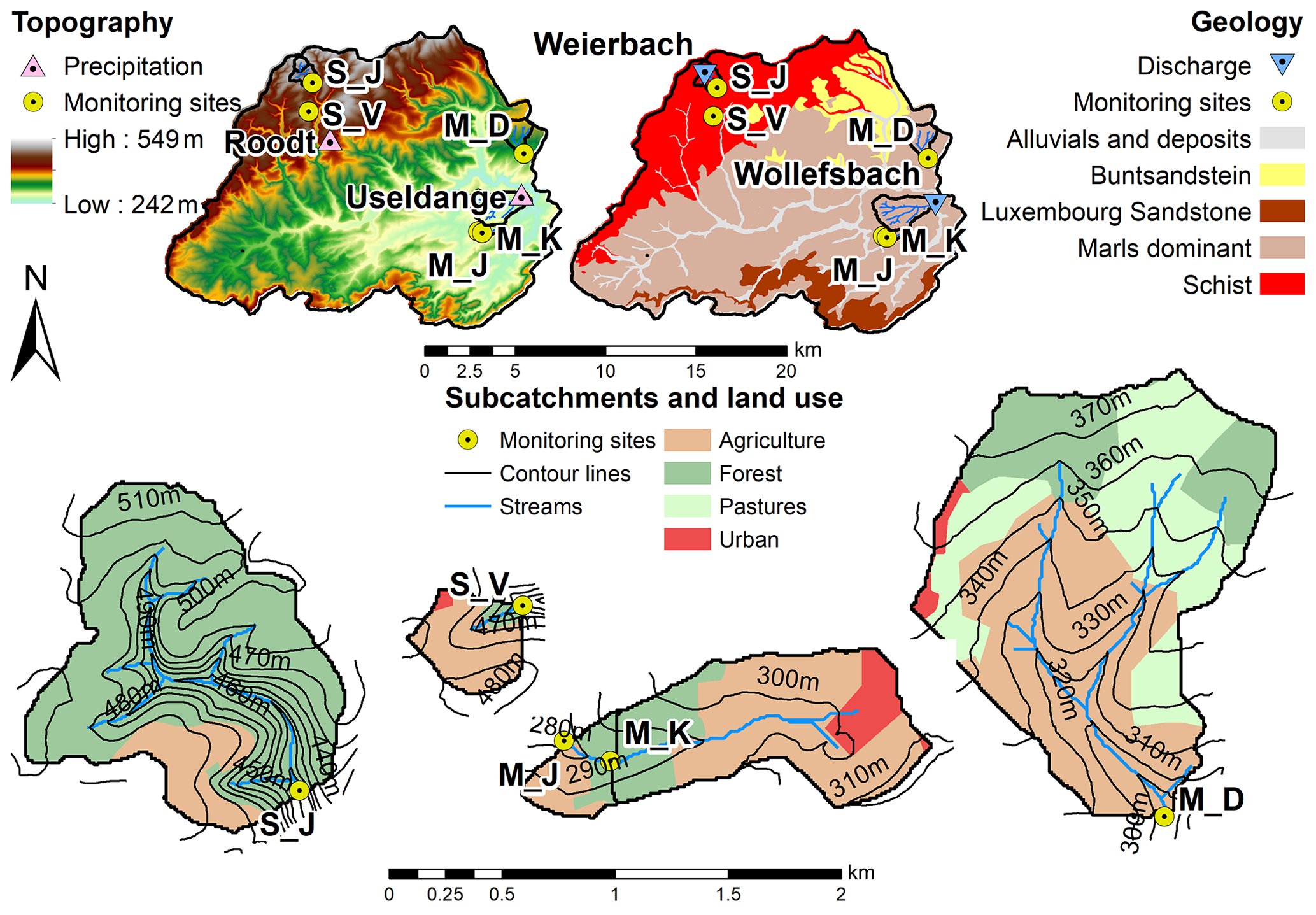
Figure 1The Attert catchment in western Luxembourg and the five monitoring sites: M_D, M_J, M_K (marls), S_J and S_V (schist). Top left is catchment topography, top right is geology and the lower half shows the five subcatchments including land use.
2.1 Study catchment
This investigation targets the 244 km2 Attert catchment in western Luxembourg, with altitudes between 243 and 549 m a.s.l. (Fig. 1, top left). It is driven by a runoff regime with generally low discharge in summer and high discharge in winter. Despite the seasonal differences in runoff, precipitation events are distributed over the entire year, with a mean annual precipitation of 760 mm.
The catchment can be divided into three main geologies – marls, schist and sandstone – and two geologies of lower significance (alluvials and Buntsandstein), shown in Fig. 1 (top right). Most of the catchment is characterised by marls and Stagnosols with high clay content (20 %–60 %), an undulating landscape and mostly agricultural land use (Sprenger et al., 2016). The high contents of clay lead to low hydraulic conductivities and a limited drainage capacity. The north-western area (Fig. 1) consists of schist bedrock and Cambisols with a texture between loam, silty loam and clayey loam, which can drain freely until the soil–bedrock interface (Sprenger et al., 2016). The landscape is here governed by elevated plateaus with mostly agricultural land use and steep forested hillslopes leading to perennial headwater streams.
A monitoring network with 45 stations was installed in the Attert catchment, recording environmental data such as climate data, soil moisture, groundwater and stream level (amongst others) (Zehe et al., 2014; Demand et al., 2019). For the investigation of hillslope–stream connectivity, we selected those monitoring sites which were situated at a stream and thus allow for a comparison between near-stream shallow groundwater level and the associated stream water level. Unfortunately no such site was available in the sandstone due to its very low drainage density, so the investigation focused on the two geologies marls and schist (Table 1 and Fig. 1, bottom). The five selected stations were put into operation between June 2012 and July 2013, and the time span until end of July 2017 was used in the analysis. The spatial arrangement of the piezometers at each site can be seen in Fig. 2, and the corresponding elevations and distances from the stream are provided in Fig. 3 and in Table A2. The prefixes M and S in the site names indicate the two geological regions. The following letter is part of the overall naming scheme of the monitoring network. A full list of the sites can be found in Appendix A of Demand et al. (2019).
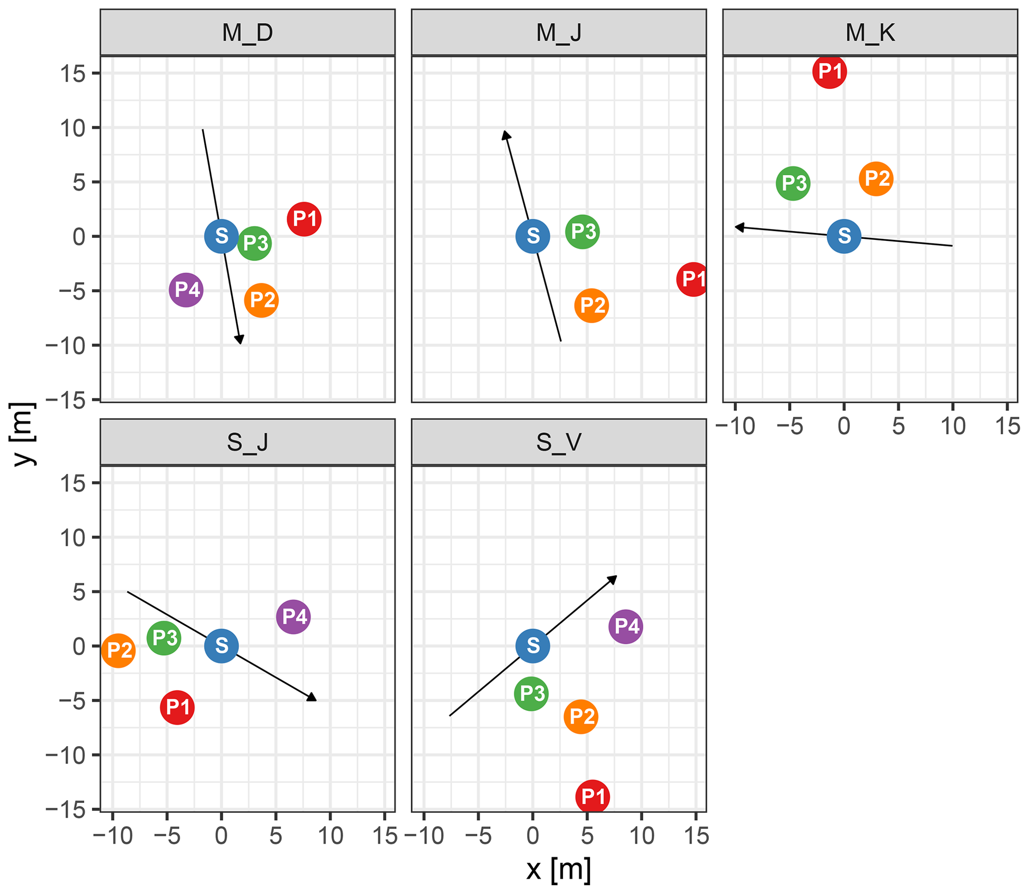
Figure 2Schematic maps of the five sites. “P” stands for piezometer with the corresponding number, while “S” stands for stream and is located at (0, 0). The arrows point along the direction of streamflow. The coordinates are relative distances to the stream water-level sensor (positive y axis points north).
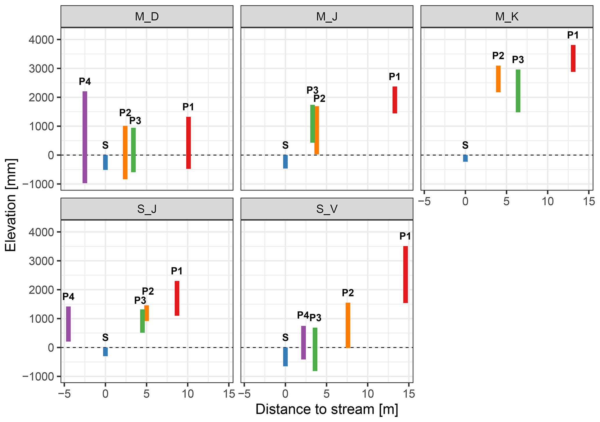
Figure 3Elevations of ground level (upper end of the bar) and sensor level (lower end) relative to the streambed. Stream sensors were installed slightly below the streambed (negative lower end). Distance to the stream is shown on the x axis. Colour coding is the same as in Fig. 2.
Table 1The basic attributes of the monitoring sites.
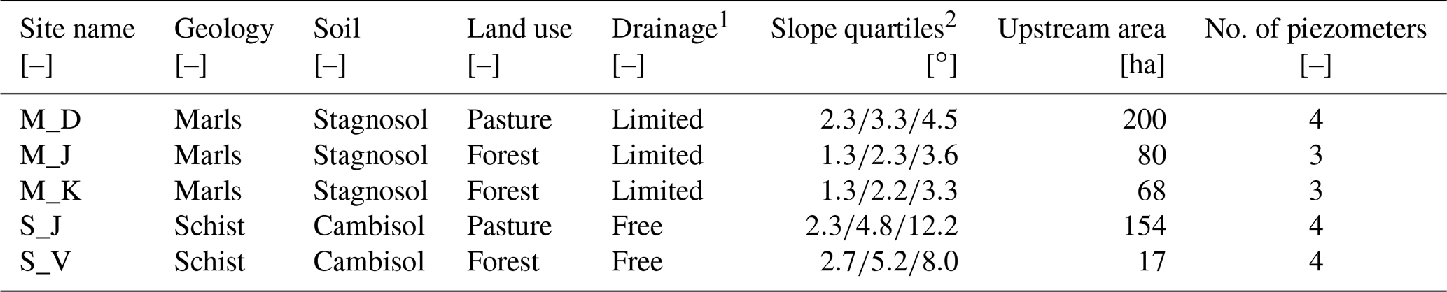
1 According to Sprenger et al. (2016). 2 Slope quartiles refer to the individual subcatchments (see Fig. 1).
M_D is located on a wide meadow with gentle inclination and piezometers 1–3 have a distance to the stream between 2 and 10 m, while piezometer 4 is on the steep opposite hillslope directly below a road cut (subsurface probably disturbed during road construction). Piezometer depths extend to about a metre below the streambed. The other two marl sites – M_J and M_K – are located in a forested plain surrounded by pasture, with the stream incised to about 2.5 m and piezometer depths of around 2 m. The horizontal distances between stream and piezometers are between 4 and 13 m for both sites. S_J is located on a small meadow floodplain, flanked by steep forested hillslopes on both sides of the stream. Piezometer depths are here around 1.5 m and reach below the streambed. Piezometers 1–3 are situated on one side of the stream with distances of about 4–8 m, while piezometer 4 is located on the other side at a distance of 6 m. S_V is located at a steep forested hillslope in a headwater catchment dominated by pasture on the higher plateau. The distance to the stream is between 2 m (piezometer 4) and 15 m (piezometer 1), and only the lower piezometers (3 and 4) extend to depths below the streambed. Average hydraulic conductivities for the two soil types range from 293 to 675 cm d−1 (Stagnosols) and from 360 to 648 cm d−1 (Cambisols) (Sprenger et al., 2016). More detailed information on the soil profiles at each piezometer can be found in Table A3.
2.2 Monitoring data
Each of the five sites described in Sect. 2.1 was equipped with three to four piezometers to measure shallow groundwater level and one sensor for stream water level. Vertical boreholes were drilled until refusal using the Cobra TT jackhammer with a hollow boring head of 75 mm diameter. Refusal was either defined as bedrock (in schist) or when a very dense layer of clay soil was reached (marls), which could not be further penetrated by the jackhammer. Perforated PVC tubing of 50 mm diameter was wrapped into non-woven fabric, installed and packed with filter gravel between 4 and 8 mm diameter. The uppermost 30 cm b.g.l. (below ground level) was packed with sealing clay to prevent infiltration bypassing the soil. Depth of refusal was in most cases below 2 m and the water level sensors were installed around 2 cm above the bottom.
The sensors used were CTD (conductivity, temperature, depth) temperature-corrected pressure transducers by METER (formerly Decagon), measuring electric conductivity, temperature and water depth. Full scale is 10 m, with a resolution of 2 mm and an accuracy of ±0.05 % of full scale. Connection cables provide ventilation to the transducer and compensate for air pressure. Automated data loggers (CR1000 by Campbell Scientific) logged the data with a temporal resolution of 5 min. Hourly precipitation data from the Roodt and Useldange weather stations were obtained from AgriMeteo Luxembourg. Both stations are located within the Attert catchment: the Roodt station being close to schist and the Useldange station being close to the marl sites (Fig. 1, upper left). Discharge data with 15 min temporal resolution were provided from the Luxembourg Institute for Science and Technology (LIST) for the Weierbach station (for schist) and the Wollefsbach station (for marls) (Fig. 1, upper right).
2.3 Event definition
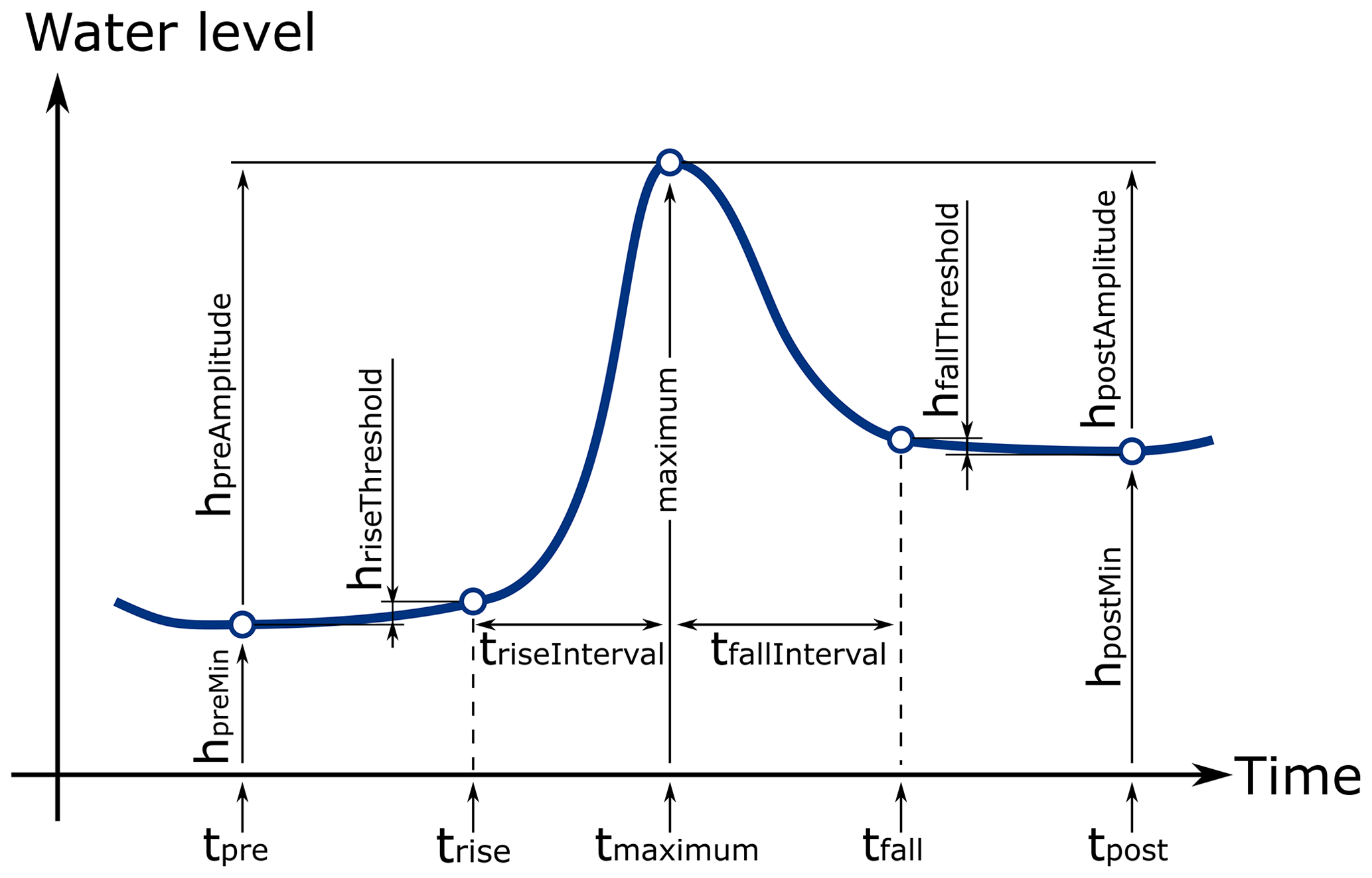
Automatic event detection is essential when working with long time series and a large number of events. To this end, it is necessary to define a generic response pattern (Fig. 4). The general response pattern begins with a pre-event minimum (hpreMin). When a precipitation event starts, the water level increases until it reaches its peak (hmaximum). After that peak, water level decreases and the event ends with a post-event minimum (hpostMin) that might differ from the pre-event minimum. These three points are used to describe water level changes during the event. However, the time period between the two minima (pre- and post-event) is not a robust measure for the event duration. Before or after events, water levels are often not stable but subject to small but misleading trends (e.g., wetting-up phase or recession). While searching for the two minima, a minimal decline has almost no effect on the water level but inappropriately increases the extracted event duration. To compensate for that, two threshold points (hriseThreshold and hfallThreshold) were introduced – one on each limb – that allow for a better temporal representation of each event. Both are defined as a certain percentage of hpreAmplitude and hpostAmplitude. In the case of the rising limb, the time where the water table exceeds hriseThreshold is called trise (see Fig. 4). Analogously, the moment the water level falls below hfallThreshold is defined as tfall. The distances to tmaximum are described as the triseInterval and tfallInterval, respectively. So for time-related analyses these two intervals are used as they are not prone to pre- and post-event trends but capture the actual event response dynamics. A percentage of 10 % of hpreAmplitude and hpostAmplitude was found to be suitable for that task.
2.4 Event detection
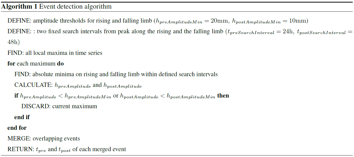
The purpose of the event detection is to parse the entire water level time series and extract those intervals during which the water level shows a response to rainfall. Algorithm 1 specifies the necessary steps for the event detection. At first, minimum amplitudes and search intervals need to be defined. Both parameters are subject to a compromise: the minimum amplitudes are used to prevent measurement noise from being mistakenly detected as events, with the drawback of possibly excluding actual low-amplitude events from detection. Search intervals are used to discriminate between subsequent events, which involves the risk of not completely capturing a very long event. In a second step, all local maxima of the stream water level are located. Thirdly, for each maximum the predefined search intervals are used in order to determine the global minima in the rising and falling limb. Defining these search intervals depends on the catchment size. Generally speaking, the search interval for the rising limb should be approximately equal to the concentration time of the subcatchment to guarantee that the complete rising limb is covered. Therefore, shorter search intervals are suited for headwaters (several hours to a day) and longer ones for lowland basins (several days). Also, the rise interval is shorter than the fall interval as such events are generally right skewed due to retention behaviour. If two or more events overlap, they are merged into one single longer event (Fig. 5) and the highest peak is determined as the event maximum. From there on, it is handled as a simple event according to Fig. 4.
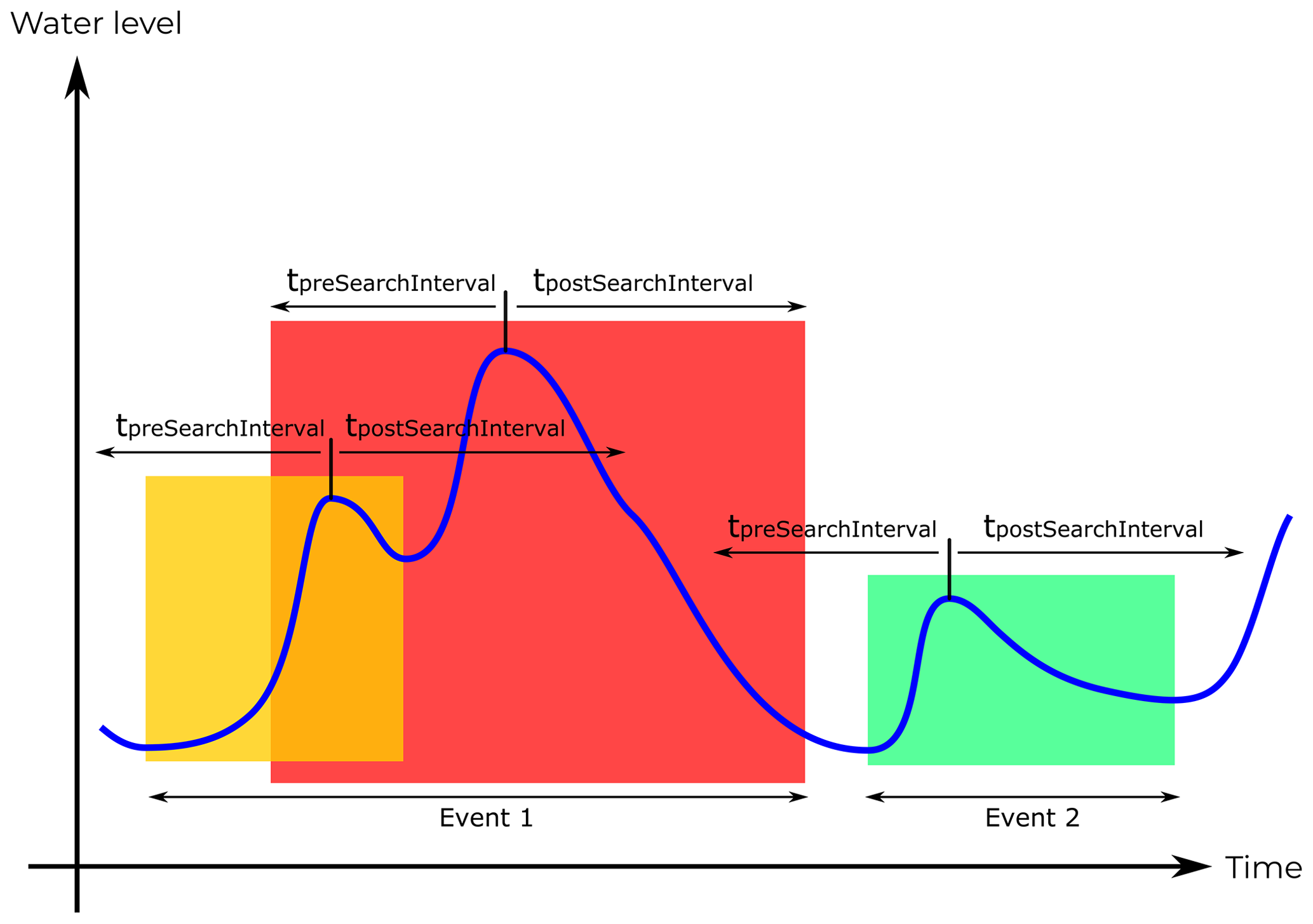
Figure 5Merging conditions of consecutive events. Time series of water level showing three local maxima and the corresponding search windows for the minima. The coloured boxes mark the independently detected events as the interval between the two absolute minima around each peak within the respective search interval. The yellow and red events overlap and are merged into one. The green event is an independent second event.
The event detection was first applied to the stream water-level time series which returns tpre and tpost for each detected stream event. For each of these stream events, a subsequent event detection is performed on the shallow groundwater level time series. Thus, we only include events in the analysis where stream water levels showed a response. Using each stream event for the detection of a possible groundwater event implies that the maximum temporal extent of the groundwater event is equal to the stream event. This is a shortcoming of this method, as a time lag between shallow groundwater and stream or drawn-out groundwater recession might lead to the predefined search window clipping the drawn-out event in the shallow groundwater. However, in the case of multiple subsequent events a clear definition must exist in order to keep a one-to-one relation between stream and groundwater events. If no temporal boundaries were applied for subsequent event detections, an event in the shallow groundwater might overlap with two or more stream events which would drastically increase the complexity of the analysis. Because of the relatively small distances of less than 15 m between stream and piezometers (and the small headwater catchments), response delays between stream and piezometer are presumed to be rather short, reducing the risk of clipping. Also, taking tpre and tpost as the temporal extent for subsequent detections in groundwater provides a buffer for potential lag times. This one-to-one approach is considered most appropriate as it is a trade-off between good operability of the detection algorithm and a high coverage of stream and groundwater events.
Amplitude thresholds were chosen via trial and error to prevent diurnal stream water fluctuations caused by root water uptake from provoking (erroneous) events. The threshold for the rising limb (20 mm) is greater than for the falling limb (10 mm), because during the wetting-up phase (in autumn) post-event water levels are very often higher than the pre-event water levels as the catchment becomes more saturated. However, on shorter timescales wetting-up can also occur in other seasons. Using the same threshold for rising and falling limb would lead to the rejection of small events with such a behaviour.
Search intervals were estimated by testing a range of values. A fixed time of 24 h for the rising limb performed satisfactorily in our catchments even for long precipitation events and did not merge several subsequent events into one bulk event. With 48 h for the falling limb, the retention behaviour of the catchment was taken into account, allowing for a long-tailed recession in comparison to the rise. The detection algorithm was run for each site individually, as a result the number and selection of detected events is site specific.
2.5 Event type
Introducing event type descriptors allows us to infer specific characteristics of a site and its experimental setup. The total number of events for a certain site is defined by its stream response, regardless of whether or not the shallow groundwater responds during the stream events. We have defined five event types: Complete, Partial, Dry, noLocalMaximum and lowAmplitudes. The Complete detections arise when the water level sensor was initially submerged and the occurring event fulfils the stated detection criteria. For Partial detections, the criteria are met but the piezometer is initially dry, so it is unknown how far below the sensor level the event started. Dry events are events where the piezometer is dry during the stream event and does not record any response. If no local maximum could be found in the groundwater during a stream event, the type was set to noLocalMaximum. lowAmplitudes means that the rise and/or fall amplitude thresholds are not surpassed. This might be due to a very low-amplitude response but can also cover events with a high rise amplitude but low fall amplitude, in particular when the peak is very close to the tpost boundary, which signals a long time lag between stream and groundwater. allNA indicates technical sensor problems in the piezometers during the detected streamflow event. While only complete events contain valid state and timing variables that can be put into relation with the stream (and are subsequently used for the detailed analyses), all non-complete events also contain relevant information. Knowing about the frequency of occurrence of these other event types helps us to characterise each piezometer and site.
2.6 Event analysis
The event analysis aims for a better understanding of how and under which conditions the shallow groundwater connects to the stream or disconnects from it. Observing the relation of water table dynamics between stream and shallow groundwater can reveal connectivity patterns which in turn give insight into the underlying processes. This simultaneous view on groundwater and stream is what is defined as the groundwater–stream (response) relation. A many-event approach ensures that a high variability of catchment conditions and response behaviours is incorporated into the analysis to cover the entire bandwidth of hydrologic system behaviour. Analyses covering single or a low number of events lack the ability of estimating variability and do not allow us to deduce how “typical” or “extreme” the event is or if it is representative.
Because the problem is multidimensional and considerably complex, a strategy was chosen that allowed us to examine various aspects of the hydrologic responses independently. Combining the information of these different aspects should then give a deeper insight into the occurring processes that control the various hillslope–stream systems.
The hillslope–stream connectivity can be investigated for periods before an event starts where underlying hydrologic processes take place on more long-term (seasonal) timescales and are represented by the baseflow. As a measure for this connectivity during baseflow conditions (between events), the rank correlation of all pre-event minima (hpreMin) between each piezometer and the corresponding stream was used. To visually compare before-event relations across piezometers and sites, each sensor's water level was normalised by its minimum and maximum hpreMin value.
Equation (1) describes the normalisation and results in a values for between 0 and 1. To indicate whether the normalised water level is above (stream) or below ground level (piezometers), the value 1 was subtracted when groundwater levels were normalised. This results in values for between −1 and 0 for groundwater.
In hillslope–stream systems infiltration and runoff generation processes are highly dynamic during events on a timescale of hours and days. To gain additional insight into what happens during these periods, we chose to handle the water level changes and timing as two separate aspects. This provides us with a view of the temporal behaviour on the one hand and changes in the state variables (water levels) of the hydrologic system on the other.
Relative timing and lags between groundwater and stream responses extracted from a large number of events hint at causal relationships. To investigate the variability of this relative timing across all events, piezometers and sites, the response behaviour was reduced to timing effects only. A very similar normalisation approach as in Eq. (1) was used to compare timings of groundwater responses with those of the stream. Equation (2) uses the time at which the stream exceeds the 10 % threshold trise stream and the time where it reaches its peak tmax stream to normalise groundwater and stream event timing.
This stream-based normalisation leads to a value of 0 for the trise in the stream and 1 for the tmaximum. A corresponding groundwater event that starts at 0 and reaches its maximum at 1 has the exact same timing as the stream. Values below 0 correspond to a time before the stream responded, while values above 1 correspond to a time where the stream already is in recession. By applying this normalisation, it is possible to compare relative time lags between stream and groundwater as well as differences in the duration.
The extent of water level increases in stream and groundwater and the relationship between the two can provide useful information on the dominant runoff generation processes. We would expect that a given increase in groundwater level at a given depth would result in a more or less predetermined/deterministic increase of stream water level (assuming the groundwater fluctuations are representative of the catchment). This means that if events A and B have similar initial conditions and cause similar groundwater level rises, we would expect the stream water level rise of event A to be the same as for event B. In this case one observation could be used to predict the other. As this also assumes that there is a connection between groundwater and stream and that runoff generation is controlled by shallow groundwater contributions, deviations from deterministic relationships are an indication of other runoff generation processes or flow path variability. Removing the temporal component and only focusing on the extent of the increase between pre-event water level and peak water level enables us to inspect this relationship.
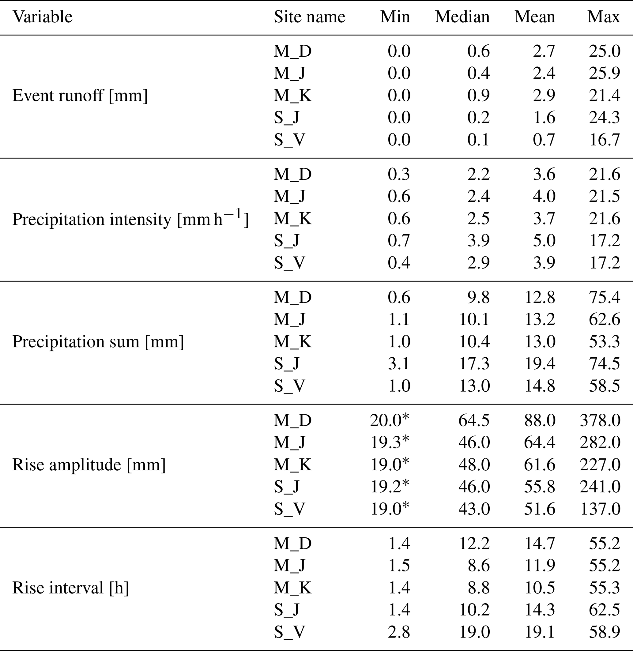
To investigate if shallow groundwater observations at a given hillslope can be used as a proxy for the state of connectivity in the entire catchment, we analysed the relationship between event runoff coefficients and the depth. The runoff coefficient describes the ratio of accumulated event discharge at the catchment outlet and accumulated catchment precipitation (Eq. 3). Even though each experimental site monitors stream level, no reliable discharge information is available since rating curves are fragmentary and thus uncertain or do not exist. Therefore, runoff coefficients (C) are calculated for nearby subcatchments (Wollefsbach and Weierbach; see Fig. 1). The spatial proximity ensures that detected stream water level events coincide with discharge events. The approach to separate baseflow from discharge is based on the constant slope method (Dingman, 2002). Baseflow (Qbaseflow(t)) was defined as the area below the straight line connecting trise and tfall and was subtracted from the total discharge (Q(t)) to calculate the actual stormflow. Precipitation (P(t)) from Roodt station was considered sufficiently representative across the Attert catchment to be used for all runoff coefficient calculations.
Relating the shallow groundwater information to the event runoff coefficients can help us to assess how representative the local measurements are for the entire catchment upstream.
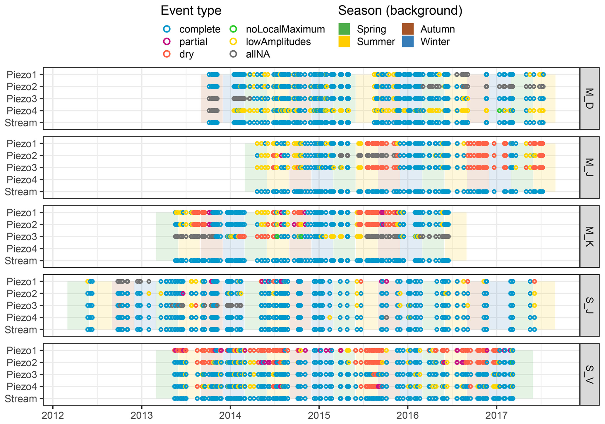
Figure 6Spatio-temporal distribution of detected events for marls (M_) and schist (S_) between June 2012 and July 2017. Seasons are defined as the periods December–February (Winter), March–May (Spring), June–August (Summer) and September–November (Autumn).
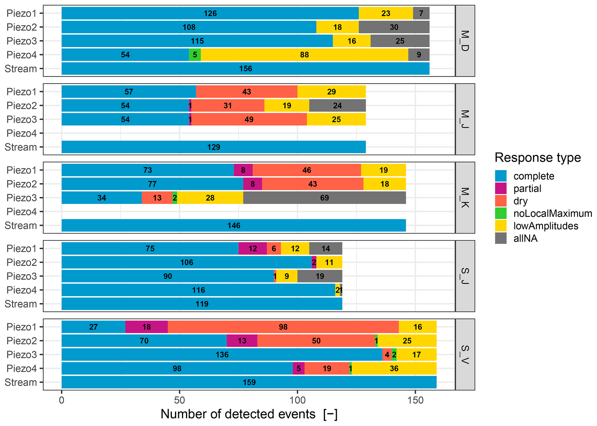
Figure 7Number of detected events in the streams and groundwater at each stream gauge and piezometer, including types of event responses.
Table 2Characteristics of the stream events summarised for each site. Different values for runoff and precipitation can occur as not all sites cover the same (number of) events. Also, different runoff and precipitation stations were used for marls and schist sites (see Fig. 1). An event runoff of 0.0 mm can occur by subtracting baseflow from total runoff.
* Threshold of 18 mm for event detection algorithm (90 % of 20 mm).
3.1 Event detection
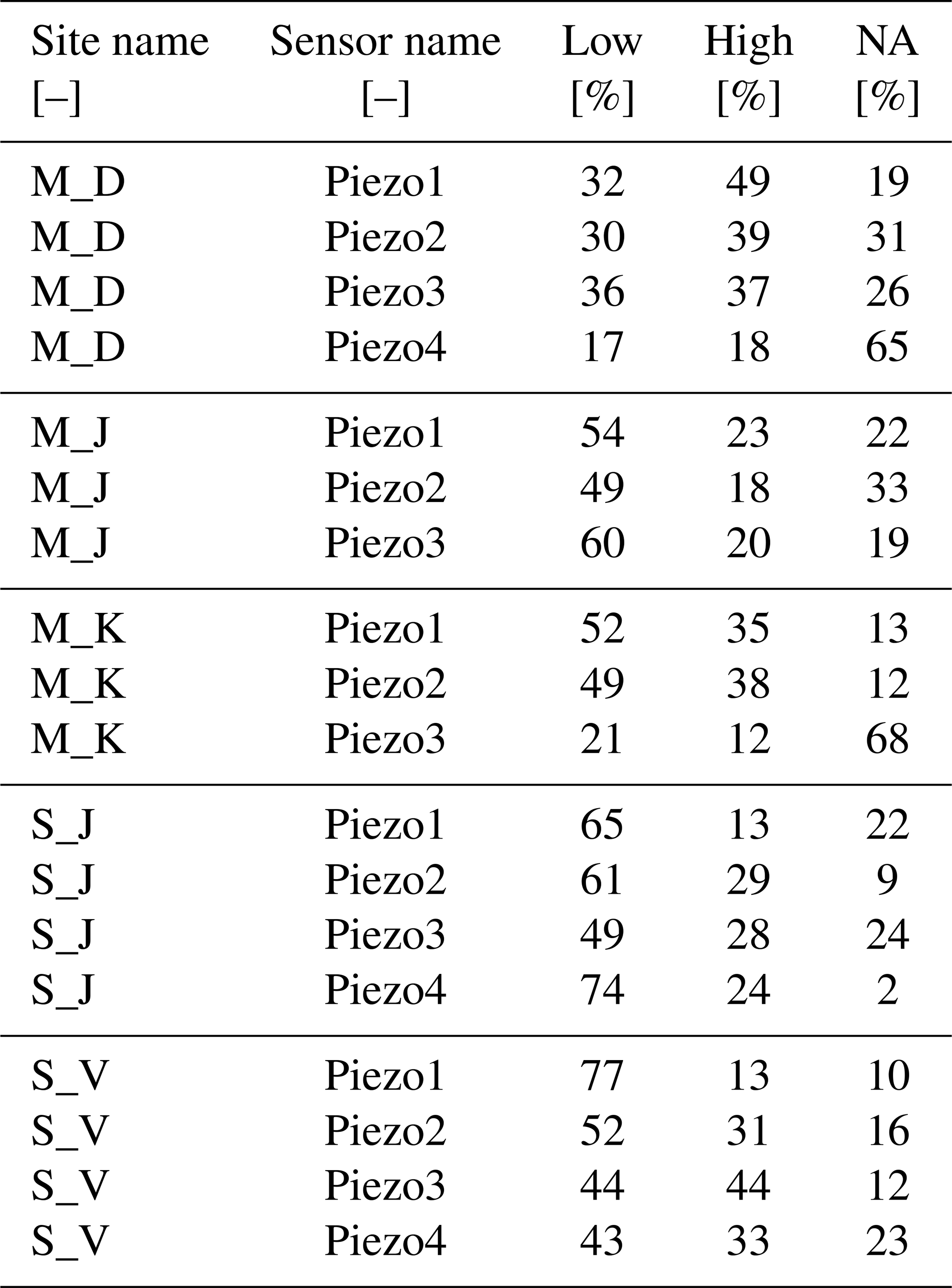
Our event detection algorithm identified between 119 and 159 stream runoff events per site over a period of 5 to 6 years. Not all of these were also detected in all piezometers (Figs. 6 and 7). This can be due to data gaps as a result of technical failure of the sensor or data gaps as the piezometer fell dry or because the response in the groundwater was strongly dampened and thus did not fulfil the criteria of the algorithm. In general, the temporal distribution of the detected events shows similar patterns across all sites (Fig. 6). It also allows us to identify M_D_Piezo4 and M_K_Piezo3 as behaving very differently with many lowAmplitudes and allNA events. In the case of lowAmplitudes, we found that many events were clipped by the predefined time window due to very long delays in relation to the stream, which were longer than in the other piezometers at these sites.
As the analysis covers winter and early spring events, the effect of snowfall and snowmelt on the event detection was assessed and found to unlikely impact our analysis. Snowfall events are generally quite rare in Luxembourg, so the number of events affected is assumed to be low. A rain-on-snow event would be captured by its runoff response, but in this case the erroneous estimate of rainfall input would only impact the analysis of event runoff coefficients as our analyses mainly focus on the relationship between streamflow and groundwater responses. Pure snowmelt events without a preceding precipitation event are not included in the analysis as precipitation is a necessary identification criterion. Referring to the response type, two main patterns can be distinguished (Fig. 6): sites where the sensors remain submerged throughout the observation period and thus produce many complete events (M_D and S_J) and sites with piezometers falling dry in summer and autumn (M_K, M_J and S_V). While at the two marl sites these dry periods occur at all piezometers concurrently, at S_V the number of dry events increases in upslope direction (from piezometer 3 to piezometer 1). The aggregated values in Fig. 7 also reveal two response types with low occurrences – namely noLocalMaximum and partial events. A total of 68 partial events were detected. The noLocalMaximum response is very rare with only 11 occurrences.
Summary statistics for precipitation, runoff and water level responses of the detected stream events are shown in Table 2. The displayed event runoff describes the total runoff minus baseflow, which can lead to a value for the event runoff of 0.0 mm.
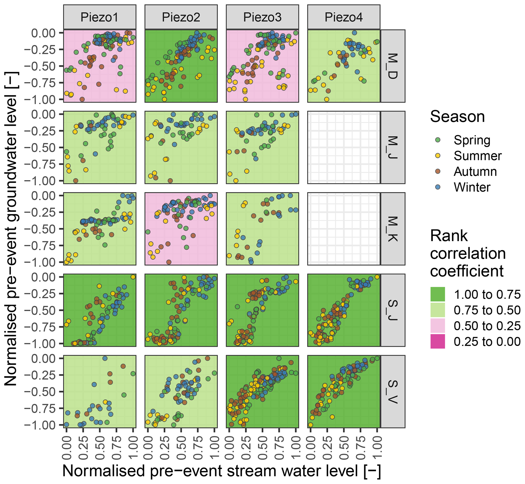
Figure 8Normalised stream and groundwater levels before the investigated precipitation events (hpreMin). The background colour represents the rank correlation coefficient, and the point colours illustrate the season. Both axes are normalised by minimum and maximum hpreMin (see Eq. 1). The negative range on the y axis indicates depths below ground (groundwater), and the positive range on the x axis indicates depths above ground (stream).
3.2 Before-event hillslope–stream connectivity
The rank correlation coefficients were found to be lower in marls than in schist sites (background colour in Fig. 8). In schist only the two upslope piezometers (Piezo1 and Piezo2) of S_V show lower correlation values (0.65 and 0.70), while the others remain above 0.80. For the three marl sites, rank correlation coefficients are generally lower (between 0.42 and 0.60) with higher variation. In marls most pre-event groundwater levels cluster in the shallow depths above −0.4 (M_K) and −0.3 (M_D and M_J). Schist groundwater levels are more evenly distributed over the entire range (Fig. 8). The point colours representing the seasons illustrate that groundwater levels are generally high in winter and spring. Summer events can be found mostly at the lower end with occasional events at higher groundwater levels. In Autumn the wetting-up phase begins, which produces events over a wider range of groundwater levels.
3.3 Comparison of relative response timing between stream and groundwater
The relative timing between groundwater and stream is illustrated in Fig. 9. The two black vertical lines represent the timing of the stream event with trise at x=0 and tmaximum at x=1. Each horizontal bar depicts a groundwater response event with its own trise at the left end and tmaximum at the right end. Groundwater responses that start at 0 and end at 1 have the exact same timing as the stream response. Starting values below 0 reveal a groundwater response before the stream, while an end value above 1 indicates that the stream is already in recession before the groundwater reaches its maximum. The events are sorted on the y axis by the normalised rise time in the groundwater from delayed groundwater response at the bottom to early groundwater response at the top. Additionally, the bar colours display the normalised pre-event water levels with high pre-event groundwater level in blue and low pre-event groundwater level in red.
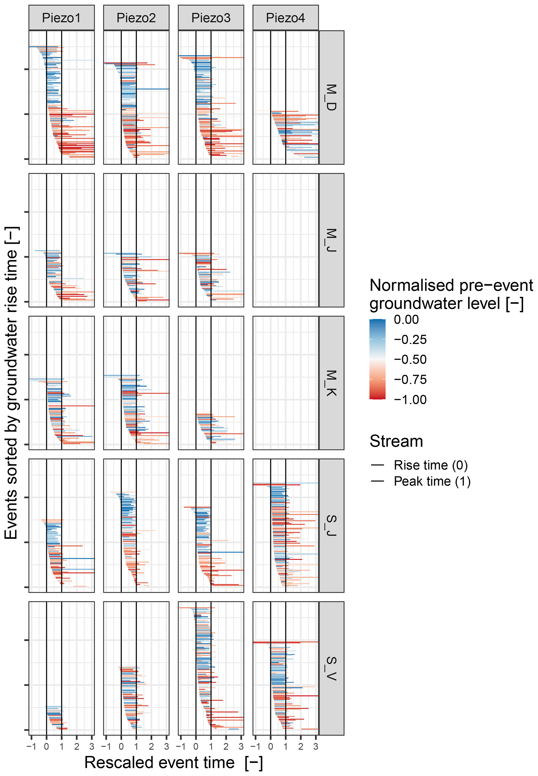
Figure 9Timing of groundwater response relative to stream response. The two vertical lines at 0 and 1 represent the normalised rise and peak time of each individual streamflow event. Horizontal bars each represent a groundwater event with its individual normalised rise and peak time. Bluish colours indicate high and reddish colours indicate low pre-event groundwater levels.
At M_D (Piezo1 to Piezo3), S_J (Piezo1 to Piezo3) and S_V (Piezo3 to Piezo4), a strong relation between pre-event groundwater levels and event timing can be observed. Events occurring at high pre-event groundwater levels (bluish) correspond with a mostly simultaneous rise in groundwater and stream, while for events at low groundwater levels (reddish) the groundwater rise lags behind the stream. Considering the peak, high groundwater events reach their maximum before or simultaneously with the stream, while during low groundwater the maximum is reached significantly after the stream. At sites M_J, M_K and S_V (Piezo1 and Piezo2), this separation of high (bluish) pre-event groundwater on top and low (reddish) pre-event groundwater at the bottom is visible but not quite as pronounced as for the other sites. In general, groundwater and stream level responses are in sync for about 20 %–60 % of the events, depending on site.
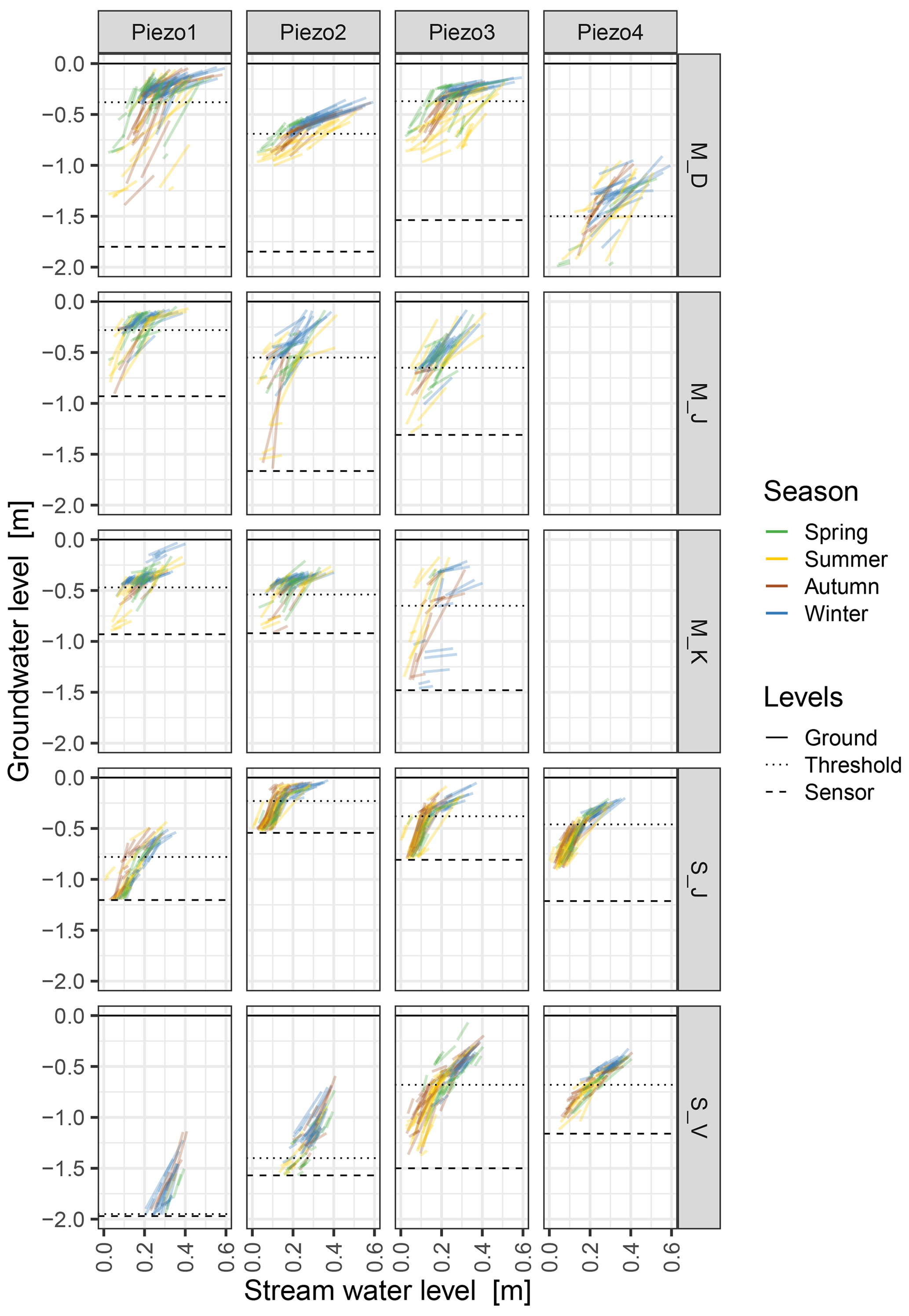
Figure 10Responses in water tables of groundwater (y axis) and the corresponding stream (x axis). The lines connect the pre-event minimum with the event maximum. Note that these water levels do not necessarily occur at the same point in time as this visualisation removes the temporal dimension. The y axis of the plot ends at a depth of 2 m for the purpose of comparison and thus omitting two events occurring below this groundwater level at M_D_Piezo4. Dotted horizontal lines illustrate the threshold between the lower (more variable but mainly steep sloping lines) and upper (less variable with shallow slopes) hydrologic response behaviour. The solid line indicates the ground surface and the dashed line the installation depth of the sensor.
3.4 Event-induced increases in stream and groundwater levels
The extent of water level increases in stream and groundwater and the relationship of the two is illustrated in Fig. 10. Both pre-event water levels (stream and groundwater) are used as coordinates for the beginning of an event line (lower left point) and the maxima as the coordinates for the end (upper left), with stream water levels on the x axis and groundwater levels on the y axis. As we removed the temporal component, it is important to keep in mind that peak values did not necessarily occur at the same time. We observe a change in response behaviour between stream and groundwater marked by a threshold which was derived visually (dotted horizontal lines) in Fig. 10. The way the patterns changed at the threshold was not identical for all sites. While many piezometers showed an abrupt change in slope (M_D Piezo1–3, M_J Piezo1 and S_J Piezo2–4), others showed their envelope functions (encompassing the bundle of slope lines) converging again. (S_J Piezo1, S_V Piezo3 and Piezo4). For some piezometers, the change in pattern was a sudden clustering of lines (M_K Piezo1–2, S_V Piezo2). All these observed changes in patterns signal that hydrologic processes do change due to different pre-event groundwater levels, when the threshold values are passed. At low groundwater levels amplitudes in the rising limb are large in the groundwater and low in the stream (steep slope of lines), while above the threshold the amplitudes in groundwater are capped at a certain depth below the surface, and stream amplitudes can become large (low slope of lines in Fig. 10). Also, the variability of pre-event conditions and event responses is larger below the threshold, while above the lines are more likely to fall on top of each other and become more deterministic. This is particularly the case for M_D (except Piezo4), M_K (except Piezo3) and S_J. Winter events cluster above the threshold and the other three seasons below the threshold and in the transition zone.
3.5 Runoff coefficient
The relation between local pre-event groundwater levels and the event runoff coefficients is displayed in Fig. 11. The dotted horizontal lines represent the same individual shallow groundwater thresholds for each piezometer identified in Fig. 10 (but here with the normalised pre-event water level on the y axis). Colours indicate whether the groundwater responded before the stream (red) or after the stream (blue). At M_D, S_J and S_V the pattern is very similar: below the individual pre-event groundwater thresholds runoff coefficients are very small but increase significantly both in value as well as in variability when pre-event groundwater levels rise above the threshold. For the two forest sites in the marls region (M_J and M_K), the pattern is less clear, with some larger runoff coefficients also occurring below the threshold. A separation with regards to relative response timing (red vs. blue) can be observed at M_D and S_J where groundwater responds before the stream for most events above the pre-event water level threshold. At the other three sites (M_J, M_K and S_V), no clear distinction can be made.
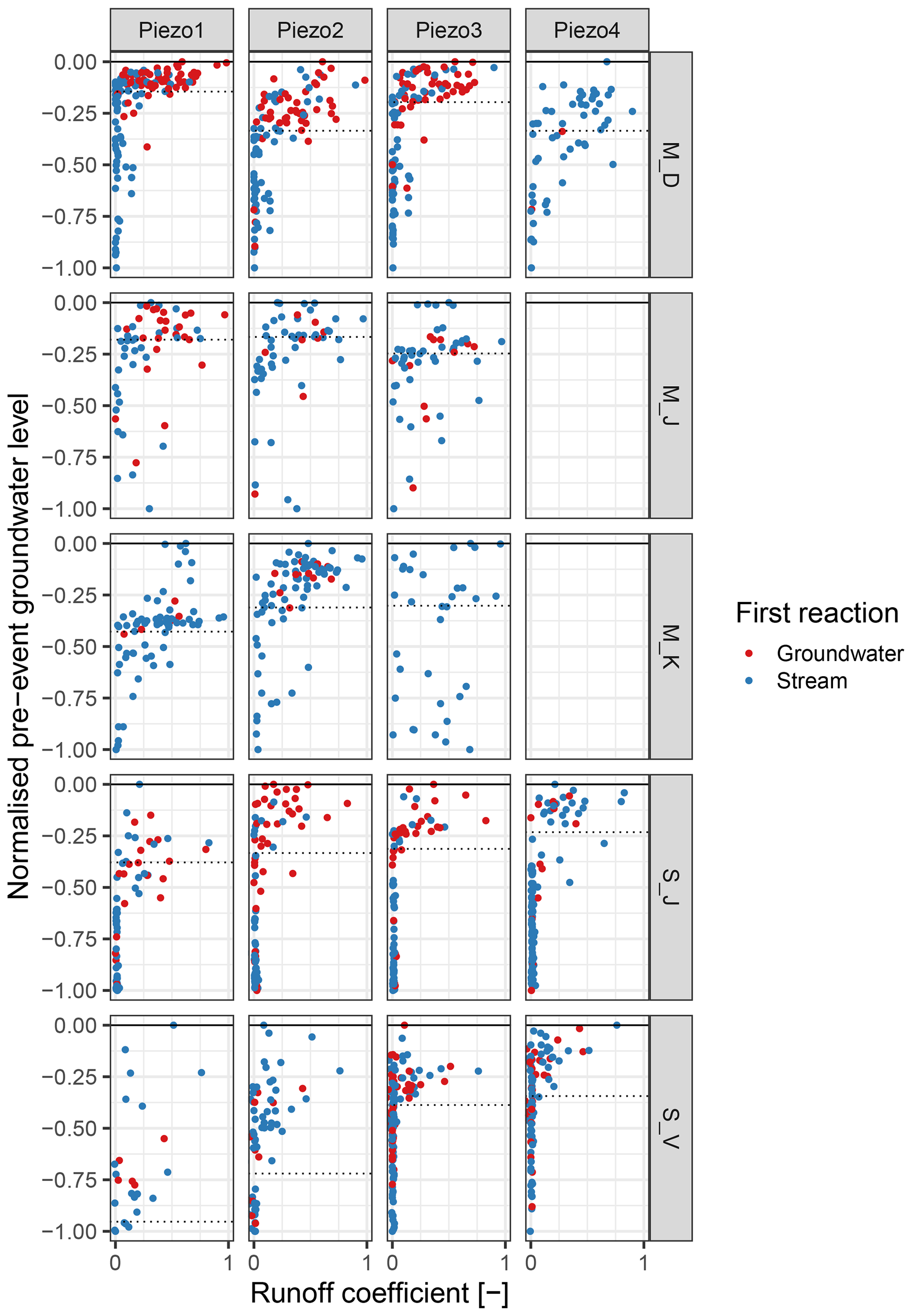
Figure 11Event runoff coefficients versus shallow groundwater levels. Event runoff coefficients were determined for the Weierbach (schist) and Wollefsbach (marls) catchments where discharge data are available. The dotted horizontal lines illustrate the individual thresholds obtained from Fig. 10. The point colours indicate whether the groundwater levels (red) or the stream (blue) responded first.
3.6 Catchment state
We assume that the threshold (Fig. 10) marks a change in catchment state, where conditions above the threshold have the potential for high connectivity, while conditions below the threshold indicate lower connectivity. To investigate if the shift in state is synchronous across the sites, we plotted the event time series colour-coded by system state (above or below the threshold) (Fig. 12). The general pattern clearly shows a common shift in hydrologic connectivity with higher probabilities of catchment states above the threshold from late autumn until early spring. However, below-threshold states can occur in winter (see, for example, the winter of 2016) and above-threshold states can also occur in summer (see, for example, summer of 2014). There is no clear distinction between the geological regions, but there are periods where system state varies across the different sites (e.g., fall 2014). However, for most events the below or above-threshold state identification is similar in timing across many piezometers.

Figure 12Catchment states at the beginning of events. In contrast to Fig. 6, it shows whether or not the groundwater levels are above (high/blue) or below (low/red) the locally defined groundwater threshold levels. Complete, partial and dry events are included; all other events are shown in grey (NA, not available).
To study the fraction of events that ended up above the threshold (Table 3), we focused on that piezometer per site that had the largest number of complete events (and excluding M_D_Piezo4 and S_J_Piezo4, which were situated on the opposite slope compared to the other piezometers at these sites). This selects Piezo1 at site M_D, Piezo2 at sites M_K and S_J, and Piezo3 at sites M_J and S_V. The fraction of streamflow events above the threshold ranges between 23 % (M_J) and 49 % (M_D). There is no relationship between the fraction of events above the threshold and geology, with M_J and S_J having the lowest fractions (<30 %) and M_D and S_V the highest fractions (>40 %). The low fraction at sites M_J, M_K and S_V_Piezo1 is in part the result of the high number of partial and dry events (in addition to the complete events below the threshold).
Table 3Fractions of events below (low, including partial and dry events) and above (high) the threshold. All other event types (lowAmplitudes, noLocalMaximum, allNA) are considered NA.
4.1 Event detection
The events summarised in Figs. 6 and 7 allow us to identify erratic sensors but also reveal topographic characteristics of the various sites. Topography can explain the occurrence of dry events, with a deeply incised stream at M_J and M_K, where we observe the lowest fraction of complete events in the groundwater with 50 % or less of the streamflow events; the steep hillslope at S_V leads to a gradient in water level depths and thus differing responses among the piezometers as well as seasonally more strongly fluctuating groundwater levels. The low numbers of partial events at sites with high numbers of complete and dry events (M_J and M_K) signal that the seasonal transition between low and high groundwater levels is very abrupt, skipping intermediate levels. This might be due to pronounced capillarity fringes reaching into the very shallow subsurface. In that case, infiltrating water would reach the upper end of the fringe very quickly and only little water volume would be necessary to lift the groundwater level significantly (e.g. Cloke et al., 2006). The very low number of only 11 noLocalMaximum groundwater events supports the viability of the developed event detection.
4.2 Before-event hillslope–stream connectivity
Cross-correlation has been used in previous studies to assess different aspects of hydrologic connectivity, such as lag time analysis between stream and groundwater table (Allen et al., 2010; Bachmair and Weiler, 2014), relating water table connectivity to topographic indices (Jencso et al., 2009) or comparing groundwater levels with runoff coefficients (Seibert et al., 2003). Assuming well coupled hydrologic systems, high correlation coefficients would be expected, which applies to the two schist sites. Low correlation coefficients indicate a streamflow (baseflow) response that is decoupled from the groundwater. This applies to all three marl sites. However, the within-site variability is not as large as the colour scheme suggests (for M_D between 0.42 and 0.76 and for M_K between 0.49 and 0.69). Visually comparing the point cloud patterns of the piezometers at each single site (Fig. 8) reveals, despite the scatter, site-internal similarity (a site-specific fingerprint) among the piezometers. Two exceptions to this observation are the previously mentioned (see Sect. 3.1) piezometer M_D_Piezo4, which is located in disturbed soil on a steep slope below a road, and M_K_Piezo3, where the anomalous behaviour can not be explained at first sight. The site-internal similarity in the point clouds as well as the rank correlation coefficients suggest that well-placed groundwater observation points can provide information on hillslope–stream connectivity for the given footslope, at least for pre-event conditions. The observed differences between the geologies suggest that soil texture and bedrock structure might control regional similarities.
4.3 Comparison of relative response timing between stream and groundwater
Identical response timing or groundwater rising and peaking just before the stream suggest that hillslope groundwater is driving streamflow response and thus that hillslope–stream connectivity is high (Haught and Meerveld, 2011; Rinderer et al., 2016). That this occurs under high groundwater levels further supports this conclusion. Groundwater rising and peaking after streamflow indicate that streamflow response is probably not caused by hillslope shallow groundwater and that hillslope–stream subsurface connectivity is low. In a highly heterogeneous catchment, certain “fast” hillslopes with very high hillslope–stream connectivity and high outflows might provoke a stream response at the stream level gauge before the monitored hillslope responds. In this case the interpretation of low subsurface connectivity would only hold for the monitored hillslope. During events with low groundwater levels, precipitation falling onto or very close to the stream might generate a rise in the stream before the groundwater response (McGuire and McDonnell, 2008), as depth of the groundwater level (minus a potential capillary fringe) is the distance a water parcel needs to travel and thus directly influences the delay in groundwater response. Triggering an early response in stream compared to groundwater can also be the result of infiltration excess overland flow where surface runoff connects faster to the stream than it infiltrates towards the groundwater. However, this can be ruled out for schist as the high infiltration capacity makes overland flow unlikely, while it can not be ruled out for the clayey soils in the marls region (Wrede et al., 2015). No clear visual differences in timing can be observed between marls and schist. The large variability in response timing confirms the need for monitoring over extended time periods as few or single event analyses run the risk of not being representative. Temporal relationship and water level responses are intertwined in a time series which makes it very intricate, focusing on one while looking at both at the same time, e.g., by plotting two time series against each other and interpreting the resulting hysteresis (Kendall et al., 1999; McGuire and McDonnell, 2010; Zuecco et al., 2016). Choosing to separate the analysis of the temporal response from the water level changes allowed us to better reveal the temporal relationship of the hillslope–stream system, on the one hand, and water level responses, on the other.
4.4 Event-induced increase in stream and groundwater levels
Previous studies observed transmissivity feedback as a key mechanism controlling subsurface runoff (Bishop et al., 2011; Detty and McGuire, 2010b). Transmissivity feedback has previously been observed directly via piezometers (Bishop et al., 2011) or indirectly through stable isotope composition in stream runoff (Bishop et al., 2004; Laudon et al., 2004) and tracer transport rates (Laine-Kaulio et al., 2014). In our study the capped response of groundwater events above a certain threshold is a strong indication of transmissivity feedback as one controlling mechanism (M_D and M_K). At low groundwater levels, infiltrating water results in a substantial increase of the groundwater level, suggesting that lateral conductivities are low as water is added more quickly than it can flow away laterally. This changes when the water level reaches a certain level or soil horizon. Now infiltrating water is no longer increasing groundwater level substantially but instead fast lateral transport is likely to be causing the observed pronounced rise in stream water levels. This sudden fast lateral transport of the shallow groundwater is likely due to substantially higher lateral hydraulic conductivity of the upper soil horizons compared to the lower soil horizons. This fits well with the findings by Sprenger et al. (2016), who at site M_K found a strong increase in saturated hydraulic conductivity by a factor of 40 at a depth of 36 cm, while the increase for site M_J (where we did not observe a strong capping of the response) is less than 20 % (the other three sites were unfortunately not included in the analysis by Sprenger et al., 2016). A raise in the hydraulic gradient in a more uniform depth profile of hydraulic conductivities, on the other hand, would only lead to a gradual increase in lateral flow. At S_V transmissivity feedback does not seem to occur as the slopes of the lines do not change as abruptly (Fig. 10). This is in accordance with the findings of Angermann et al. (2017) at the same hillslope: during sprinkling experiments they observed that relatively high vertical and lateral hydraulic conductivities (10−3 m s−1) lead to fast lateral responses in subsurface. Whether or not a precipitation event can activate certain flow paths depends on the spatial distribution of pre-event water and the characteristics of bedrock topography (van Meerveld et al., 2015). Demand et al. (2019) found that preferential flow is present in particular during dry conditions. When the groundwater level is high, the majority of flow paths are already activated and the degrees of freedom to activate new flow paths are limited. Therefore, the relation between stream and groundwater converges and shifts from variable to more uniform (Fig. 10). Investigating rainfall characteristics and their effect on event responses did not help with explaining the underlying mechanisms. While rank correlation coefficients between precipitationSum and hpreAmplitude reached relatively high values of 0.7 and above, the majority stayed below 0.2 for triseInterval, showing that the precipitation had no clearly identifiable effect on event timing (see Table A1).
4.5 Runoff coefficient
Threshold behaviour is a common observation in runoff generation (Ali et al., 2013); for example, Scaife and Band (2017) and Detty and McGuire (2010b) observed a threshold effect of antecedent precipitation and soil moisture on stormflow, and Latron and Gallart (2008) identified a threshold behaviour between groundwater level and runoff coefficient depending on seasonal catchment conditions (dry, wetting-up and wet). In our study the groundwater threshold marking the change in event runoff coefficients (Fig. 11) coincides with the regime shift of water table responses (Fig. 10). At M_D, S_J and S_V the pattern is very similar: below the individual pre-event groundwater thresholds runoff coefficients are very small but increase significantly both in value as well as in variability when pre-event groundwater levels rise above the threshold. For the two forest sites in the marls region (M_J and M_K), the pattern is less clear, with some larger runoff coefficients also occurring below the threshold. A possible explanation could be that Wollefsbach gauge used to determine the runoff coefficients is less representative for these forest sites, as the Wollefsbach catchment consists almost entirely of pasture and agricultural areas. In addition, the morphology of slopes and stream channel at the two marls forest sites is very distinct (and different to the Wollefsbach), with very low gradients in the slopes but a deeply incised streambed. As the probability of high runoff coefficients increases above the groundwater threshold, it seems that local observations of groundwater levels can give a good indication of catchment state with respect to connectivity and storage and release behaviour. This is true even for neighbouring catchments within the same geological region (M_D and S_V, for example, are not located in or downstream of the catchments used for the determination of the runoff coefficients). We also find that especially the regime shift and the corresponding threshold can be more clearly identified by groundwater level observations than by antecedent stream water level (Fig. 10). This implies that near-stream groundwater observations hold significant predictive power to estimate whether or not an upcoming precipitation event is likely to produce major runoff at the outlet of the subcatchment.
4.6 Catchment state
The previously obtained groundwater thresholds allow us to split all events into two groups: events with catchment states above the threshold are likely to have higher event runoff coefficients (Fig. 11) and are thus assumed to generate substantial lateral subsurface stormflow caused by high hillslope–stream connectivity (more connected hillslopes, connectivity extending further upslope, or both). Catchment states below the threshold generate only minor lateral flow. In this case the spatial extent of hillslope–stream connectivity is generally low (few connected hillslopes or connectivity does not extend far up the slopes). Just taking season as a predictor for the expected event response and hillslope–stream connectivity would be too simple: while summer events are likely to be below threshold and winter events above, this is not a general rule and spring and autumn events can also not be classified just by their season (Fig. 12). However, our study results suggest that it would be sufficient to have the information of one of the piezometers per site to know if pre-event groundwater levels are above or below the threshold. If a rainfall event were to occur when groundwater levels are above the threshold, the likelihood of high runoff coefficients would be increased. To identify this state (above or below threshold), we do not need all of the piezometers currently installed at a certain hillslope – one would be enough, and we could then potentially dismantle the other piezometers. Considering an un-investigated hillslope, one can not know in advance which location would lead to a “well-chosen” piezometer and which one to a “badly chosen” piezometer. Nonetheless, the analysis showed that local heterogeneity did not influence the piezometers to a degree where no similarity at all could be observed. Therefore, a small number of piezometers (e.g. 3–4) should be enough to identify the characteristic patterns and which piezometers do represent the hillslope and which ones are less suited due to local anomalies. From this point on, one piezometer would be enough to describe the hillslope response and you could remove the other sensors. The well-chosen one would be one that, on the one hand, is consistent in its response pattern with the majority of the piezometers at this site and, on the other hand, has the clearest threshold signal among these.
Even though the temporal dynamics of the switches between above- and below-threshold conditions are similar across most piezometers and sites, the fraction of stream events ending up above the threshold varies strongly (Table 3). While this only refers to the events and not the continuous time series, it still tells us that high connectivity on an event basis only occurs for roughly 20 %–50 % of the events. While we saw higher pre-event connectivity at the schist sites (deduced from the rank correlation coefficients of pre-event stream and groundwater levels Fig. 8), there was no geological pattern in the fraction of above-threshold events. These two measures describe different aspects of connectivity. While the footslope of the schist sites is well connected during pre-event conditions, this does not necessarily mean that the upslope areas at these sites are more frequently contributing to streamflow than upslope areas where the footslope is less well connected during pre-event conditions.
4.7 Synthesis: process deductions
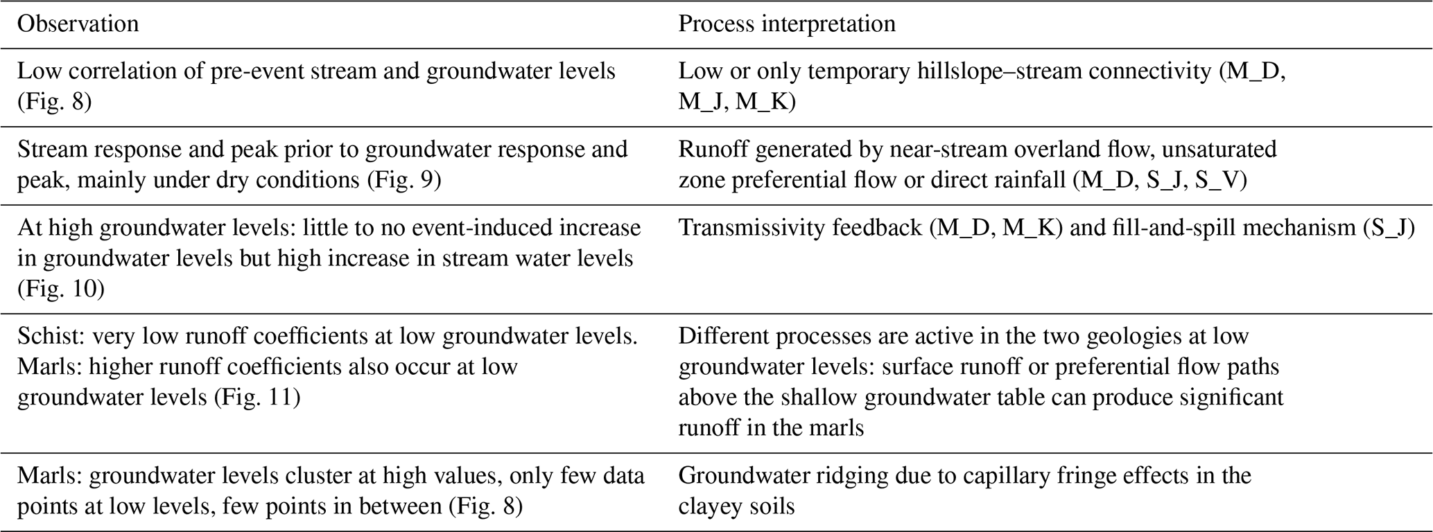
The joint analysis of shallow near-stream groundwater and stream water levels allows us to identify several runoff generation mechanisms. Observations and the corresponding interpretations are listed in Table 4.
Table 4Observations and corresponding process interpretations.
The observations described in Table 4 require a large number of events. Only if the number of events is sufficiently high can we capture the variability in responses, frequency of different response types and the dominant responses and then interpret the underlying processes (Table 5 shows a selection of studies with the number of events analysed).
Detty and McGuire (2010b)Ali et al. (2011)Penna et al. (2015)Anderson et al. (2010)van Meerveld and McDonnell (2006a)Scaife and Band (2017)Rinderer et al. (2016)Zuecco et al. (2019)Table 5Selection of studies and the number of events analysed.
Events in marls cluster at high pre-event groundwater levels with 60 % to 80 % of events found in the upper half of the total range and only few events at low levels or in between. At the same time, the piezometers at M_J and M_K experience a considerably high number of dry events but only few partial events (Fig. 7). Groundwater transitions fast from very low levels to levels near the surface, with only few events in between (Fig. 8). This fast transition hints towards extended capillary fringes where only low volumes of water are necessary to rise the groundwater table (Cloke et al., 2006). As a result of the transmissivity feedback, runoff coefficients significantly increase when groundwater levels reach the threshold as the hillslope connects to the stream (Fig. 11). This behaviour can be observed in particular at the largest catchment in marls (M_D) with an undulating landscape and mostly pasture and to a lesser degree at smaller catchments with very flat topography and forest. As several characteristics are different between these catchments, this behaviour can not be assigned to one single attribute with confidence. In schist, events are spread over the whole range of pre-event groundwater levels with no clear difference between low, in-between and high events. Since hydraulic conductivities in schist are generally very high; the sudden increase in runoff coefficient above the threshold can not be explained by transmissivity feedback being the governing process. Nevertheless, capping of groundwater response was observed at S_J. Anderson et al. (2010) found that in watersheds with lateral preferential flow, the fill-and-spill mechanism was responsible for capped groundwater responses. This observation can be transferred to the schist site to explain the inhibited groundwater response making its soil–bedrock interface responsible for the threshold relationship.
Studies focusing on the downslope travel distances (Klaus and Jackson, 2018; Gabrielli and McDonnell, 2020) found that only lower regions of a hillslope contribute to the streamflow via interflow, while in upper regions water percolates into the deeper groundwater. In our study, however, we find that there is a threshold in the near-stream groundwater levels above which event runoff coefficients rise strongly to values above 50 %, indicating that it is not just the near-stream footslope contributing to event runoff.
In this study we analysed the relation between responses to precipitation of shallow groundwater level and stream level for five different sites in two distinct geologies. An event-based approach was chosen for the analysis of the multiannual time series where responses in water level and timing were investigated independently. We found that a multi-event analysis approach including a large number of events is suitable for characterising the hydrologic response behaviour of the hillslope-stream system and the dynamics of its connectivity. A more selective and exemplary analysis of only a few events would lead to misinterpretation of the results. Nonetheless, the question is not so much about how many events are necessary (in absolute numbers) but more about the necessary time period to cover the temporal variability generated by different hydrological processes. It is therefore necessary to accumulate a large number of events across all seasons. In terms of extreme events (droughts or floods) the covered time period and number of events will need to be even higher, on the one hand, to capture these events and, on the other hand, to put them into context. Detecting threshold behaviour and identifying the correct threshold would be very unlikely if the above conditions would not be met. Thus, the lack of information on event variability would significantly reduce the confidence of the findings (see figures in Appendix B).
Revisiting our hypotheses, we now can say the following:
-
Hypothesis 1. Hillslopes remain disconnected from the stream for most of the time and connect only during short periods of time.
We found that the fraction of events above the threshold (with the potential of high runoff coefficients) was roughly 20 %–50 % of the streamflow events, depending on site. Similarly, the relative timing between groundwater and stream level response was very much in sync for 20 %–60 % of the streamflow events, again depending on site. However, as even the events above the threshold do not all produce high runoff coefficients, we are unable to falsify the hypothesis. Instead our results indicate that indeed, even though the footslopes might be connected, the hillslopes are often disconnected. Pronounced and continuous foot-slope–stream connectivity during baseflow conditions is therefore not an indicator of frequently occurring upslope contributions.
-
Hypothesis 2. The two geologies (schist and marls) differ in topography and soil characteristics. As a result, their hillslope–stream systems will show differing connectivity patterns.
Differences between the response behaviour of the two geologies were less pronounced than expected for some of the analyses, but the observed results showed that both hydrologic systems are subject to a threshold behaviour where dominating hydrologic processes change. While both geologies show threshold behaviour the underlying processes are likely to be different, with transmissivity feedback occurring in the marls and a more fill-and-spill-like process in the schist. The fact that at low groundwater levels runoff coefficients in the marls tend to be higher than in the schist, in some cases even by an order of magnitude, suggests that also at low groundwater levels different processes are active in the two geological regions. While saturated subsurface connectivity is low at these low groundwater levels, surface runoff or lateral preferential flow above the shallow groundwater must provide sufficient connectivity to enable runoff generation in the marls. Interestingly, the two schist sites showing high pre-event connectivity of stream and footslope had strongly differing fractions of events above the threshold. On the other hand, site M_D had low pre-event connectivity but a 49 % fraction of events above the threshold.
-
Hypothesis 3. Monitoring at the footslope can provide information on hillslope–stream connectivity at this location and can indicate connectivity at the headwater catchment scale.
Our analyses identified patterns that are representative for the site or hillslope, i.e., which were shown by all or most piezometers at these sites. However, piezometers can also be located at points where very local anomalies drastically influence the response behaviour which is why at least three piezometers should be used when first investigating the hillslope–stream relation to secure redundant information and identify the most representative and informative monitoring location for the hillslope or even catchment. Then a single, well-chosen, piezometer can already provide substantial information on catchment state and the potential for high connectivity and thus high runoff events. This conclusion is based on the fact that piezometer water levels above the identified threshold can be related to an increased potential for high event runoff coefficients which in turn indicate increased catchment connectivity. Thus the piezometer water levels above the threshold are indicative of a catchment storage state at which additional rainwater input can easily lead to a strong increase in catchment connectivity and thus runoff production.
The proposed separation of the temporal component and the extent of water level responses for certain aspects of the data analysis proved to be useful in visualising, analysing and interpreting the event response and its variability across a large number of events. Even though the installation and monitoring of piezometers in the near-stream zone is pragmatic and much less cost- and labour-intensive than the installation of hillslope trenches, local near-stream shallow groundwater observations do hold significant predictive power for the potential catchment response. They possibly provide more information than piezometer or trench observations located further upslope would, as the footslope and riparian zone are both link and gatekeeper, controlling connectivity between hillslopes and streams. Due to the lower cost of piezometer installation and monitoring compared to trenches, it is possible to instrument a larger number of sites which in turn makes it possible to systematically investigate subsurface hillslope–stream connectivity in different hydrologic response units instead of focusing on within-slope connectivity on single hillslopes. While we focused on five hillslopes in this study, it would easily be possible to extend this monitoring design to a larger number of sites and thus even better capturing the spatial variability in responses and allowing a thorough investigation into which sites tend to be most representative of the catchment and if these sites can be identified a priori based on topography or other landscape characteristics. The application of our data analysis to other sites where data are already available might open up new ways of systematic site-intercomparison as our analysis provides a novel way of visualising event responses and thus making the information contained in a large number of events more easily accessible.
Table A1Spearman rank correlation coefficients between event precipitation and the response variables riseAmplitude and riseInterval.

Figure B1Normalised stream and groundwater levels. Black events are from 2015, while grey events are from all other years. (Replotting of Fig. 8 to visualize the effect of a reduced (1-year) observation period.)
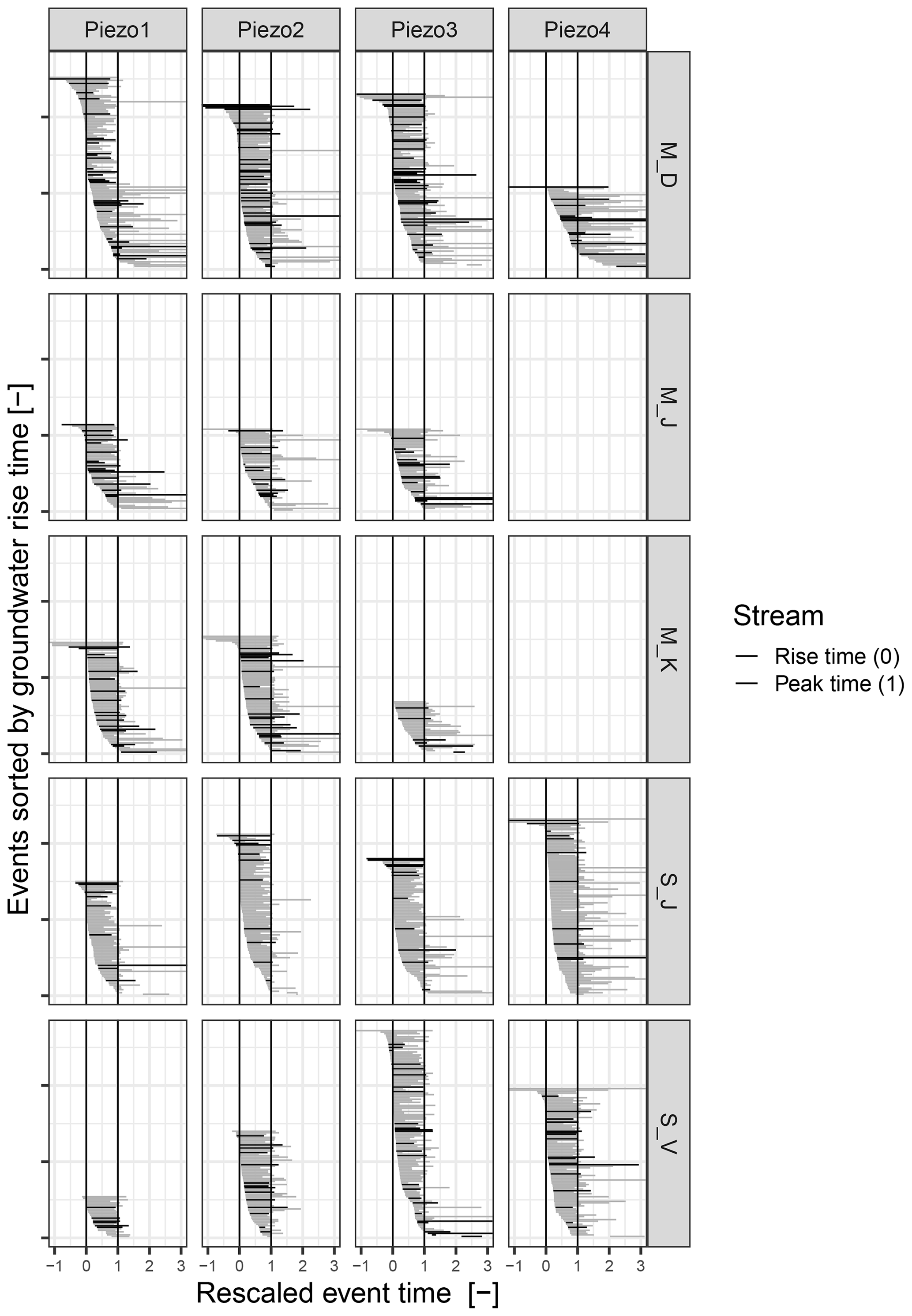
Figure B2Timing of groundwater response relative to stream response. Black events are from 2015, while grey events are from all other years. (Replotting of Fig. 9 to visualize the effect of a reduced (1-year) observation period.)
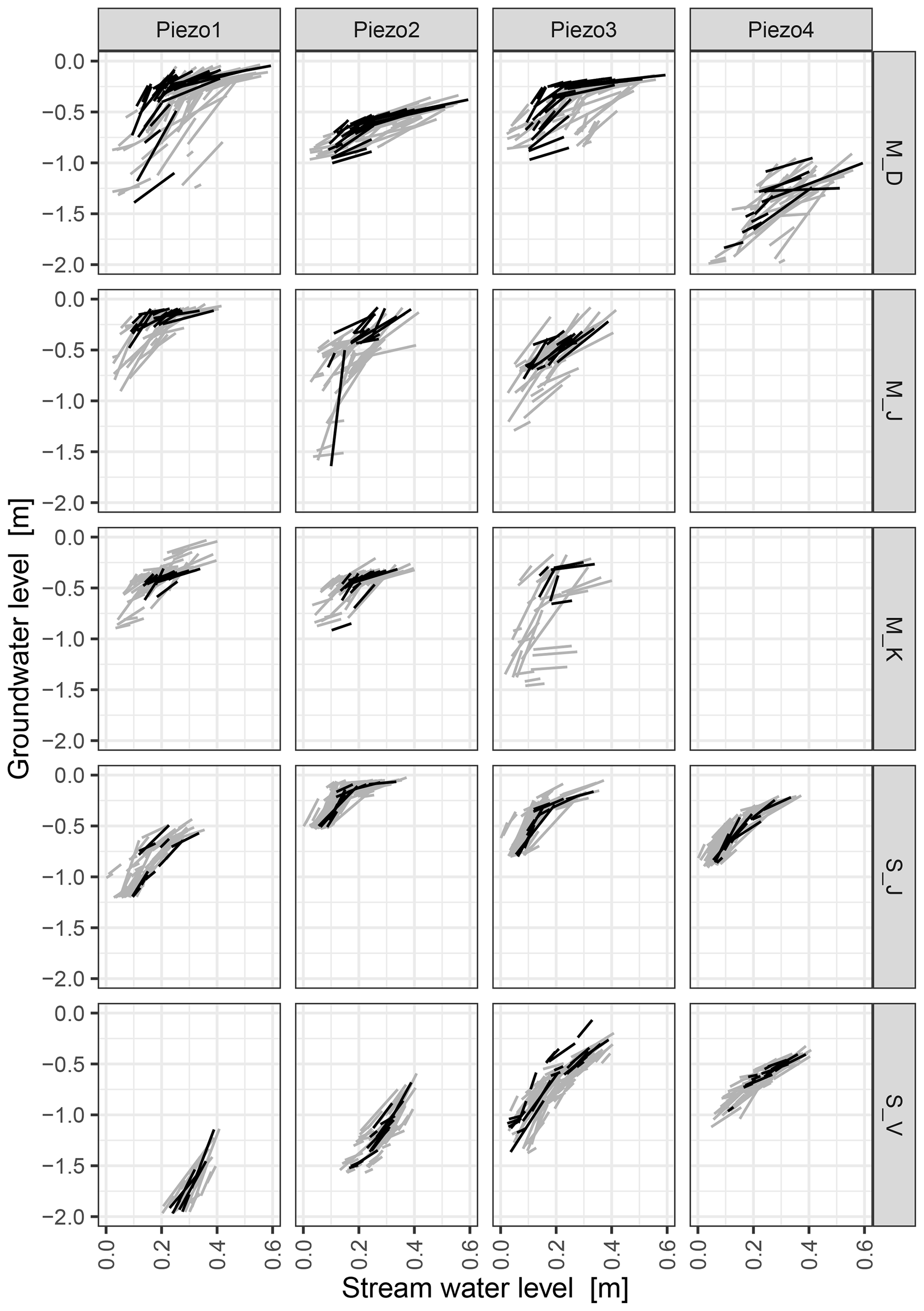
Figure B3Responses in water tables of groundwater (y axis) and the corresponding stream (x axis). Black events are from 2015, while grey events are from all other years. (Replotting of Fig. 10 to visualize the effect of a reduced (1-year) observation period.)

Data will be made available in a corresponding data publication in ESSD.
None of the authors have financial competing interests; however, authors Markus Weiler and Theresa Blume are members of the editorial board of the journal.
This article is part of the special issue “Linking landscape organisation and hydrological functioning: from hypotheses and observations to concepts, models and understanding (HESS/ESSD inter-journal SI)”. It is not associated with a conference.
We gratefully acknowledge DFG for the research funding (FOR 1598) and thank the group of Laurent Pfister at the Luxembourg Institute of Technology (LIST) for providing the discharge data, AgriMeteo for the precipitation data, Matthias Sprenger for the soil horizon data, and Tobias Vetter and Britta Kattenstroth for their untiring maintenance of the monitoring sites.
This research has been supported by the DFG, German Research Foundation (grant Research Unit CAOS – Catchments as Organized Systems, FOR 1598).
The article processing charges for this open-access
publication were covered by a Research
Centre of the Helmholtz Association.
This paper was edited by Hjalmar Laudon and reviewed by four anonymous referees.
Ali, G., Oswald, C. J., Spence, C., Cammeraat, E. L., McGuire, K. J., Meixner, T., and Reaney, S. M.: Towards a unified threshold-based hydrological theory: necessary components and recurring challenges, Hydrol. Process., 27, 313–318, 2013. a
Ali, G. A. and Roy, A. G.: Revisiting Hydrologic Sampling Strategies for an Accurate Assessment of Hydrologic Connectivity in Humid Temperate Systems, Geogr. Compass, 3, 350–374, https://doi.org/10.1111/j.1749-8198.2008.00180.x, 2009. a
Ali, G. A., L'Heureux, C., Roy, A. G., Turmel, M.-C., and Courchesne, F.: Linking spatial patterns of perched groundwater storage and stormflow generation processes in a headwater forested catchment, Hydrol. Process., 25, 3843–3857, https://doi.org/10.1002/hyp.8238, 2011. a, b
Allen, D. M., Whitfield, P. H., and Werner, A.: Groundwater level responses in temperate mountainous terrain: regime classification, and linkages to climate and streamflow, Hydrol. Process., 24, 3392–3412, https://doi.org/10.1002/hyp.7757, 2010. a
Anderson, A. E., Weiler, M., Alila, Y., and Hudson, R. O.: Piezometric response in zones of a watershed with lateral preferential flow as a first-order control on subsurface flow, Hydrol. Process., 24, 2237–2247, https://doi.org/10.1002/hyp.7662, 2010. a, b, c, d, e
Anderson, S. P., Dietrich, W. E., Montgomery, D. R., Torres, R., Conrad, M. E., and Loague, K.: Subsurface flow paths in a steep, unchanneled catchment, Water Resour. Res., 33, 2637–2653, https://doi.org/10.1029/97WR02595, 1997. a
Angermann, L., Jackisch, C., Allroggen, N., Sprenger, M., Zehe, E., Tronicke, J., Weiler, M., and Blume, T.: Form and function in hillslope hydrology: characterization of subsurface flow based on response observations, Hydrol. Earth Syst. Sci., 21, 3727–3748, https://doi.org/10.5194/hess-21-3727-2017, 2017. a
Bachmair, S. and Weiler, M.: Interactions and connectivity between runoff generation processes of different spatial scales, Hydrol. Process., 28, 1916–1930, https://doi.org/10.1002/hyp.9705, 2014. a, b, c
Bishop, K., Seibert, J., Köhler, S., and Laudon, H.: Resolving the double paradox of rapidly mobilized old water with highly variable responses in runoff chemistry, Hydrol. Process., 18, 185–189, 2004. a
Bishop, K., Seibert, J., Nyberg, L., and Rodhe, A.: Water storage in a till catchment. II: Implications of transmissivity feedback for flow paths and turnover times, Hydrol. Process., 25, 3950–3959, 2011. a, b
Blume, T. and van Meerveld, H. I.: From hillslope to stream: methods to investigate subsurface connectivity, Wiley Interdisciplin. Rev.: Water, 2, 177–198, https://doi.org/10.1002/wat2.1071, 2015. a
Bracken, L., Wainwright, J., Ali, G., Tetzlaff, D., Smith, M., Reaney, S., and Roy, A.: Concepts of hydrological connectivity: Research approaches, pathways and future agendas, Earth-Sci. Rev., 119, 17–34, https://doi.org/10.1016/j.earscirev.2013.02.001, 2013. a
Cloke, H., Anderson, M., McDonnell, J., and Renaud, J.-P.: Using numerical modelling to evaluate the capillary fringe groundwater ridging hypothesis of streamflow generation, J. Hydrol., 316, 141–162, 2006. a, b
Creed, I. F. and Band, L. E.: Exploring functional similarity in the export of Nitrate-N from forested catchments: A mechanistic modeling approach, Water Resour. Res., 34, 3079–3093, https://doi.org/10.1029/98WR02102, 1998. a
Demand, D., Blume, T., and Weiler, M.: Spatio-temporal relevance and controls of preferential flow at the landscape scale, Hydrol. Earth Syst. Sci., 23, 4869–4889, https://doi.org/10.5194/hess-23-4869-2019, 2019. a, b, c
Detty, J. M. and McGuire, K. J.: Topographic controls on shallow groundwater dynamics: implications of hydrologic connectivity between hillslopes and riparian zones in a till mantled catchment, Hydrol. Process., 24, 2222–2236, https://doi.org/10.1002/hyp.7656, 2010a. a, b
Detty, J. M. and McGuire, K. J.: Threshold changes in storm runoff generation at a till-mantled headwater catchment, Water Resour. Res., 46, W07525, https://doi.org/10.1029/2009WR008102, 2010b. a, b, c, d, e, f
Dingman, S.: Physical Hydrology, Prentice Hall, University of New Hampshire, New Hampshire, available at: https://books.google.de/books?id=BHAeAQAAIAAJ (last access: 3 October 2019), 2002. a
Freer, J., McDonnell, J. J., Beven, K. J., Peters, N. E., Burns, D. A., Hooper, R. P., Aulenbach, B., and Kendall, C.: The role of bedrock topography on subsurface storm flow, Water Resour. Res., 38, 5-1–5-16, https://doi.org/10.1029/2001WR000872, 2002. a, b, c
Gabrielli, C. P. and McDonnell, J. J.: Modifying the Jackson index to quantify the relationship between geology, landscape structure, and water transit time in steep wet headwaters, Hydrol. Process., 34, 2139–2150, https://doi.org/10.1002/hyp.13700, 2020. a
Graham, C. B., Woods, R. A., and McDonnell, J. J.: Hillslope threshold response to rainfall: (1) A field based forensic approach, J. Hydrol., 393, 65–76, https://doi.org/10.1016/j.jhydrol.2009.12.015, 2010. a, b, c
Haught, D. R. W. and Meerveld, H. J.: Spatial variation in transient water table responses: differences between an upper and lower hillslope zone, Hydrol. Process., 25, 3866–3877, https://doi.org/10.1002/hyp.8354, 2011. a, b, c
Hornberger, G. M., Bencala, K. E., and McKnight, D. M.: Hydrological controls on dissolved organic carbon during snowmelt in the Snake River near Montezuma, Colorado, Biogeochemistry, 25, 147–165, https://doi.org/10.1007/BF00024390, 1994. a
Jackson, C. R. and Pringle, C. M.: Ecological Benefits of Reduced Hydrologic Connectivity in Intensively Developed Landscapes, BioScience, 60, 37–46, https://doi.org/10.1525/bio.2010.60.1.8, 2010. a
Jencso, K. G., McGlynn, B. L., Gooseff, M. N., Wondzell, S. M., Bencala, K. E., and Marshall, L. A.: Hydrologic connectivity between landscapes and streams: Transferring reach- and plot-scale understanding to the catchment scale, Water Resour. Res., 45, w04428, https://doi.org/10.1029/2008wr007225, 2009. a
Jencso, K. G., McGlynn, B. L., Gooseff, M. N., Bencala, K. E., and Wondzell, S. M.: Hillslope hydrologic connectivity controls riparian groundwater turnover: Implications of catchment structure for riparian buffering and stream water sources, Water Resour. Res., 46, W10524, https://doi.org/10.1029/2009WR008818, 2010. a
Kendall, K., Shanley, J., and McDonnell, J.: A hydrometric and geochemical approach to test the transmissivity feedback hypothesis during snowmelt, J. Hydrol., 219, 188–205, https://doi.org/10.1016/S0022-1694(99)00059-1, 1999. a
Klaus, J. and Jackson, C. R.: Interflow Is Not Binary: A Continuous Shallow Perched Layer Does Not Imply Continuous Connectivity, Water Resour. Res., 54, 5921–5932, https://doi.org/10.1029/2018WR022920, 2018. a
Krause, S., Blume, T., and Cassidy, N. J.: Investigating patterns and controls of groundwater up-welling in a lowland river by combining Fibre-optic Distributed Temperature Sensing with observations of vertical hydraulic gradients, Hydrol. Earth Syst. Sci., 16, 1775–1792, https://doi.org/10.5194/hess-16-1775-2012, 2012. a
Laine-Kaulio, H., Backnäs, S., Karvonen, T., Koivusalo, H., and McDonnell, J. J.: Lateral subsurface stormflow and solute transport in a forested hillslope: A combined measurement and modeling approach, Water Resour. Res., 50, 8159–8178, 2014. a
Latron, J. and Gallart, F.: Runoff generation processes in a small Mediterranean research catchment (Vallcebre, Eastern Pyrenees), J. Hydrol., 358, 206–220, https://doi.org/10.1016/j.jhydrol.2008.06.014, 2008. a
Laudon, H., Seibert, J., Köhler, S., and Bishop, K.: Hydrological flow paths during snowmelt: Congruence between hydrometric measurements and oxygen 18 in meltwater, soil water, and runoff, Water Resour. Res., 40, W03102, https://doi.org/10.1029/2003WR002455, 2004. a
McGlynn, B. L. and McDonnell, J. J.: Quantifying the relative contributions of riparian and hillslope zones to catchment runoff, Water Resour. Res., 39, 1310, https://doi.org/10.1029/2003wr002091, 2003. a
McGuire, K. and McDonnell, J.: Stable Isotope Tracers in Watershed Hydrology, in: chap. 11, John Wiley & Sons, Ltd, Oxford, 334–374, https://doi.org/10.1002/9780470691854.ch11, 2008. a
McGuire, K. J. and McDonnell, J. J.: Hydrological connectivity of hillslopes and streams: Characteristic time scales and nonlinearities, Water Resour. Res., 46, W10543, https://doi.org/10.1029/2010WR009341, 2010. a, b, c
Ocampo, C. J., Sivapalan, M., and Oldham, C.: Hydrological connectivity of upland-riparian zones in agricultural catchments: Implications for runoff generation and nitrate transport, J. Hydrol., 331, 643–658, https://doi.org/10.1016/j.jhydrol.2006.06.010, 2006. a, b
Oswald, C. J., Richardson, M. C., and Branfireun, B. A.: Water storage dynamics and runoff response of a boreal Shield headwater catchment, Hydrol. Process., 25, 3042–3060, https://doi.org/10.1002/hyp.8036, 2011. a
Penna, D., Mantese, N., Hopp, L., Dalla Fontana, G., and Borga, M.: Spatio-temporal variability of piezometric response on two steep alpine hillslopes, Hydrol. Process., 29, 198–211, https://doi.org/10.1002/hyp.10140, 2015. a, b
Rinderer, M., van Meerveld, I., Stähli, M., and Seibert, J.: Is groundwater response timing in a pre-alpine catchment controlled more by topography or by rainfall?, Hydrol. Process., 30, 1036–1051, 2016. a, b
Scaife, C. I. and Band, L. E.: Nonstationarity in threshold response of stormflow in southern Appalachian headwater catchments, Water Resour. Res., 53, 6579–6596, https://doi.org/10.1002/2017WR020376, 2017. a, b, c, d
Seibert, J., Bishop, K., Rodhe, A., and McDonnell, J. J.: Groundwater dynamics along a hillslope: A test of the steady state hypothesis, Water Resour. Res., 39, 1014, https://doi.org/10.1029/2002wr001404, 2003. a
Sprenger, M., Seeger, S., Blume, T., and Weiler, M.: Travel times in the vadose zone: Variability in space and time, Water Resour. Res., 52, 5727–5754, https://doi.org/10.1002/2015wr018077, 2016. a, b, c, d, e, f
Thompson, J., Cassidy, R., Doody, D. G., and Flynn, R.: Predicting critical source areas of sediment in headwater catchments, Agr. Ecosyst. Environ., 179, 41–52, 2013. a
van Meerveld, H. J. T. and McDonnell, J. J.: Threshold relations in subsurface stormflow: 1. A 147-storm analysis of the Panola hillslope, Water Resour. Res., 42, W02410, https://doi.org/10.1029/2004wr003778, 2006a. a
van Meerveld, H. J. T. and McDonnell, J. J.: Threshold relations in subsurface stormflow: 2. The fill and spill hypothesis, Water Resour. Res., 42, w02411, https://doi.org/10.1029/2004wr003800, 2006b. a, b, c, d, e, f
van Meerveld, H. J., Seibert, J., and Peters, N. E.: Hillslope–riparian-stream connectivity and flow directions at the Panola Mountain Research Watershed, Hydrol. Process., 29, 3556–3574, https://doi.org/10.1002/hyp.10508, 2015. a, b
Wrede, S., Fenicia, F., Martínez-Carreras, N., Juilleret, J., Hissler, C., Krein, A., Savenije, H. H. G., Uhlenbrook, S., Kavetski, D., and Pfister, L.: Towards more systematic perceptual model development: a case study using 3 Luxembourgish catchments, Hydrol. Process., 29, 2731–2750, https://doi.org/10.1002/hyp.10393, 2015. a
Zehe, E., Ehret, U., Pfister, L., Blume, T., Schröder, B., Westhoff, M., Jackisch, C., Schymanski, S. J., Weiler, M., Schulz, K., Allroggen, N., Tronicke, J., van Schaik, L., Dietrich, P., Scherer, U., Eccard, J., Wulfmeyer, V., and Kleidon, A.: HESS Opinions: From response units to functional units: a thermodynamic reinterpretation of the HRU concept to link spatial organization and functioning of intermediate scale catchments, Hydrol. Earth Syst. Sci., 18, 4635–4655, https://doi.org/10.5194/hess-18-4635-2014, 2014. a
Zuecco, G., Penna, D., Borga, M., and van Meerveld, H.: A versatile index to characterize hysteresis between hydrological variables at the runoff event timescale, Hydrol. Process., 30, 1449–1466, 2016. a
Zuecco, G., Rinderer, M., Penna, D., Borga, M., and van Meerveld, H. J.: Quantification of subsurface hydrologic connectivity in four headwater catchments using graph theory, Sci. Total Environ., 646, 1265–1280, https://doi.org/10.1016/j.scitotenv.2018.07.269, 2019. a
- Abstract
- Introduction
- Methods
- Results
- Discussion
- Conclusions
- Appendix A: Additional information on rainfall effects and piezometer and profile characteristics
- Appendix B: Visualisation of information loss when monitoring only 1 year instead of multiple years
- Data availability
- Competing interests
- Special issue statement
- Acknowledgements
- Financial support
- Review statement
- References