Comparison of root water uptake models in simulating CO₂ and H₂O fluxes and growth of wheat

Stomatal regulation and whole plant hydraulic signaling affect water fluxes and stress in plants. Land surface models and crop models use a coupled photosynthesis–stomatal conductance modeling approach. Those models estimate the effect of soil water stress on stomatal conductance directly from soil water content or soil hydraulic potential without explicit representation of hydraulic signals between the soil and stomata. In order to explicitly represent stomatal regulation by soil water status as a function of the hydraulic signal and its relation to the whole plant hydraulic conductance, we coupled the crop model LINTULCC2 and the root growth model SLIMROOT with Couvreur's root water uptake model (RWU) and the HILLFLOW soil water balance model. Since plant hydraulic conductance depends on the plant development, this model coupling represents a two-way coupling between growth and plant hydraulics. To evaluate the advantage of considering plant hydraulic conductance and hydraulic signaling, we compared the performance of this newly coupled model with another commonly used approach that relates root water uptake and plant stress directly to the root zone water hydraulic potential (HILLFLOW with Feddes' RWU model). Simulations were compared with gas flux measurements and crop growth data from a wheat crop grown under three water supply regimes (sheltered, rainfed, and irrigated) and two soil types (stony and silty) in western Germany in 2016. The two models showed a relatively similar performance in the simulation of dry matter, leaf area index (LAI), root growth, RWU, gross assimilation rate, and soil water content. The Feddes model predicts more stress and less growth in the silty soil than in the stony soil, which is opposite to the observed growth. The Couvreur model better represents the difference in growth between the two soils and the different treatments. The newly coupled model (HILLFLOW–Couvreur's RWU–SLIMROOT–LINTULCC2) was also able to simulate the dynamics and magnitude of whole plant hydraulic conductance over the growing season. This demonstrates the importance of two-way feedbacks between growth and root water uptake for predicting the crop response to different soil water conditions in different soils. Our results suggest that a better representation of the effects of soil characteristics on root growth is needed for reliable estimations of root hydraulic conductance and gas fluxes, particularly in heterogeneous fields. The newly coupled soil–plant model marks a promising approach but requires further testing for other scenarios regarding crops, soil, and climate.

1 Introduction

Soil water status is amongst the key factors that influence photosynthesis, evapotranspiration, and growth processes (Hsiao, 1973). Accurate estimation of crop water stress responses is important for predictions of crop growth, yield, and water use by crop models and land surface models (Egea et al., 2011).

Crop models and land surface models lump the effects of soil water deficit on stomatal regulation and crop growth in so-called “stress factors” (Verhoef and Egea, 2014; Mahfouf et al., 1996). Crop water stress is strongly influenced by soil water availability, which in turn depends on the distribution of water and of roots in the root zone and the transpiration rate or total root water uptake. Adequate representations in simulation models of root water uptake (hereafter RWU) and root distributions (Gayler et al., 2013; Wöhling et al., 2013; Zeng et al., 1998; Desborough, 1997) are therefore needed. Most macroscopic RWU models estimate the water uptake as a function of potential transpiration (i.e., the transpiration of the crop when water is not limited) and average moisture content or soil water pressure head and rooting densities (Feddes et al., 2001; van Dam, 2000). However, in this representation of RWU, crucial relations between RWU model parameters and root and plant hydraulic conductances, which translate the soil water pressure head to water hydraulic heads in the shoot to which stomata respond, are lost. Note that hydraulic heads refer to total water potentials expressed in length units and pressure heads to the hydraulic head minus the gravitational potential or elevation. For instance, the water stress factor calculated by the Feddes model (Feddes et al., 1978) based on the soil water pressure heads involves indirect linkages between the root zone water pressure head and the hydraulic head in the shoot in the sense that the water stress factors are adapted when the potential transpiration rate changes. Such models like the Feddes approach represent the role of the root and plant hydraulic conductance indirectly and thus require calibration for different crop types and growing seasons (Cai et al., 2018; Vandoorne et al., 2012; Wesseling et al., 1991). The conductance of the root system is an important feature of the root system and different approaches to include it in RWU models were published (Quijano and Kumar, 2015; Vadez, 2014, Kramer and Boyer, 1995; Peterson and Steudle, 1993). Plant hydraulic conductance determines leaf water potentials which have a significant impact on stomatal conductance, leaf gas exchange, and leaf growth (Tardieu et al., 2014; Trillo and Fernández, 2005; Sperry, 2000; Zhao et al., 2005; Gallardo et al., 1996). Recently, some one-dimensional macroscopic RWU models based on hydraulic principles have been developed to represent water potential gradients from the soil to roots (de Jong van Lier et al., 2008) and within the root system (Couvreur et al., 2014). The latter approach simplified a physically based description of water flow in the coupled soil–root system accounting for the root system hydraulic properties and architecture to simple linear equations between soil water pressure heads, the leaf water hydraulic head, root water uptake profiles, and the transpiration rate that can be solved directly. It thereby avoids computation of time-consuming numerical solutions of ordinary differential equations for the water flow and balance in the root system that are coupled with the nonlinear soil water balance partial differential equation. It uses a stomatal regulation model that assumes that stomatal conductance is not influenced by the leaf water hydraulic head as long as the leaf hydraulic head is above a critical leaf hydraulic threshold. The leaf water hydraulic head is kept constant by changing stomatal conductance when the critical leaf hydraulic threshold is reached. The Couvreur model also allows the different stomatal regulations to be presented (i.e., isohydric and anisohydric in Tardieu and Simonneau, 1998) (Couvreur et al., 2014, 2012).

Recently, inverse modeling routines using datasets of root density, leaf area, and soil water content and potential permitted the quantification of root-related parameters of Couvreur's model (root hydraulic conductivity). Sap flow measurements were used to validate simulated RWU using the parameterized model (Cai et al., 2017, 2018). These studies demonstrated the close relation between the root system conductance and root growth as part of overall plant growth and its response to water stress pointing at a two-way coupling between root water uptake and plant growth. This implies that the parameterization of root water uptake needs to be coupled to plant growth, which in turn is influenced by water stress and other factors. Plant hydraulic conductance was introduced in crop models for several field crops such as soybean (Olioso et al., 1996) and winter wheat (Wang et al., 2007) or for model testing (Tuzet et al., 2003). However, plant hydraulic conductance in these studies was kept constant without reference to dynamic root growth. To the best of our knowledge, the effect of two-way coupling between a RWU model accounting for whole plant hydraulic regulation and a crop growth model has not been studied yet. It is unclear whether such a coupled model improves the simulation of crop growth and development and CO₂ and H₂O fluxes.

In this study, we coupled Couvreur's RWU model (Couvreur et al., 2012, 2014) with the existing crop growth model LINTULCC2 (Rodriguez et al., 2001) to consider the whole plant hydraulic conductance from root to shoot. The dynamics of root and shoot growth under varying soil water availability are explicitly represented by the coupled model. The overall aim of the study was to investigate whether consideration of plant hydraulic conductance can improve the simulation of CO₂ and H₂O fluxes and crop growth in biomass, roots, and leaf area index of the same crop that is grown in two different soils and for three different water application regimes. To achieve this aim, three objectives were addressed: (i) to analyze and compare the predictive quality of a crop growth model coupled with a RWU model that considers plant hydraulics (Couvreur RWU model) and a model that does not consider plant hydraulics (Feddes RWU model); (ii) to compare the simulated plant hydraulic conductances for the different growing conditions with direct estimates of these conductances from measurements; and (iii) to analyze the sensitivity of RWU and crop growth to the Couvreur RWU and root growth model parameters (root hydraulic conductance, critical leaf hydraulic threshold, and specific weight of seminal and lateral roots).

2 Materials and methods

2.1 Location and experimental setup

The study area was located in Selhausen in North Rhine-Westphalia, Germany (50^∘52^′ N, 6^∘27^′ E). The study field is slightly inclined with a slope of around 4^∘ and characterized by a strong gradient in stone content along the slope (Stadler et al., 2015). Two rhizotrones were set up in the field: the upper site with stony soil (hereafter F1) contains up to 60 % gravel by weight, while in the lower site with silty soil (hereafter F2) the gravel content was approximately 4 %. At each study site the effects of three different water treatments on growth and fluxes were investigated (sheltered – P1, rainfed – P2, and irrigated – P3) (Fig. 1). Each treatment was 3.25 m wide and 7 m long. The treatments bordered each other along the 7 m long side. Further information on the field experiment and setup are presented in Cai et al. (2016, 2018) and Stadler et al. (2015). Irrigation was applied two times: on 22 and 26 May 2016 in the irrigated plots (F1P3 and F2P3) during the growing season using dripper lines. The dripper lines (model T-Tape 510-20-500, Wurzelwasser GbR, Münzenberg, Germany) were installed at 0.3 m intervals and parallel to crop rows. The nontransparent plastic shelter was manually covered (11 times) during rainfall and removed when rain stopped to induce water stress. On the sheltered days, radiation was assumed to be zero for the sheltered plots. Winter wheat (Triticum aestivum `Ambello') was sown with a density of 350–370 seeds m⁻² on 26 October 2015 and harvested on 26 July 2016 in both the stony (F1) and silty (F2) parts of the field. Fertilizers were applied at a rate of 80 kg N + 60 kg K₂O + 30 kg P₂O₅ ha⁻¹ on 15 March 2016. Nitrogen was further added on 2 May and 7 June 2016 at 60 and 50 kg N ha⁻¹, respectively. Weeds and pests were controlled according to standard agronomic practice.

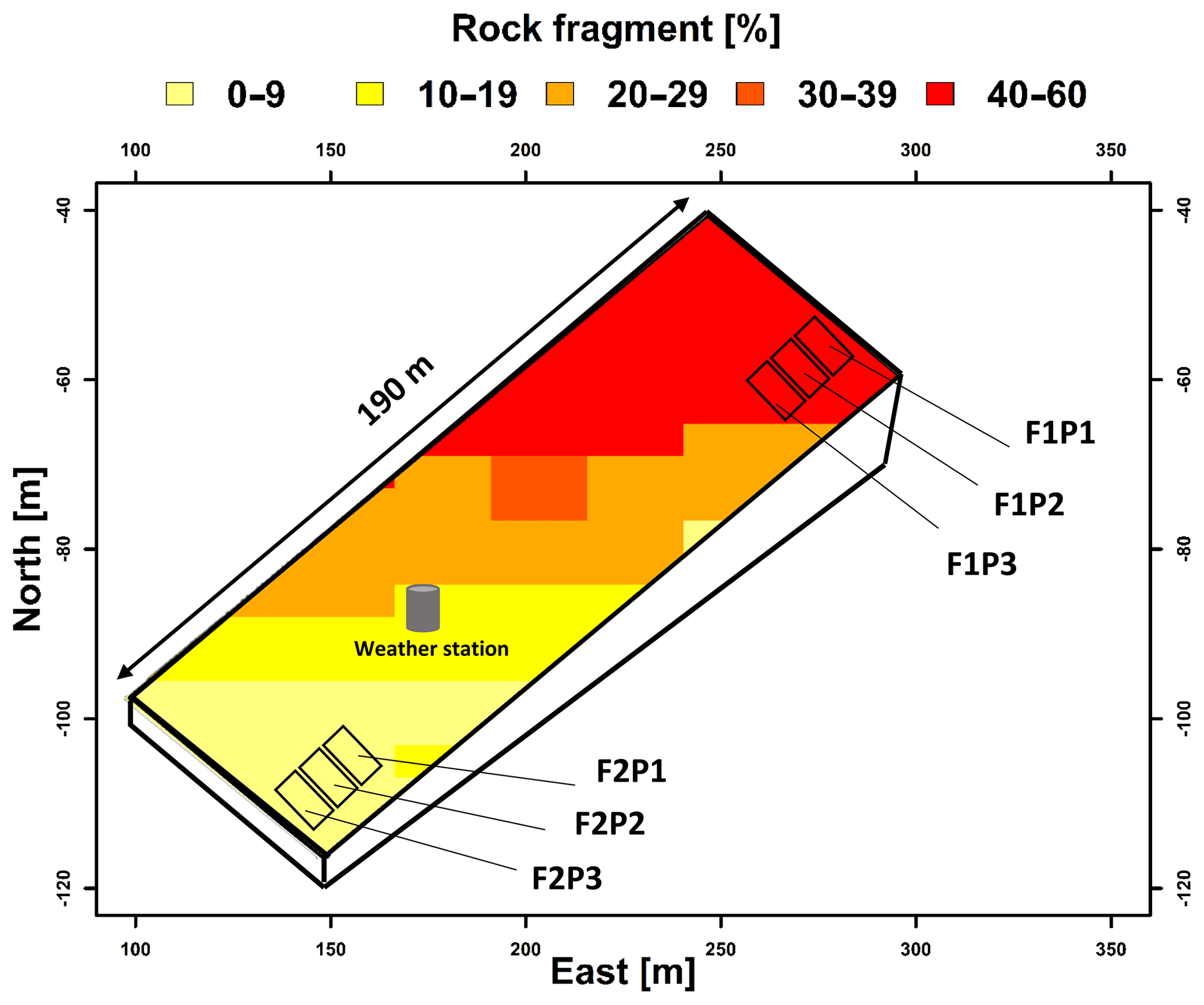
Figure 1 Description of the location of field experiment and setup of water treatments in the stony soil (F1) and silty soil (F2). P1–P3 are the sheltered, rainfed, and irrigated plots. Rock fragments are gravels with weathered granites.

2.2 Measurements

2.2.1 Soil water measurement and root growth

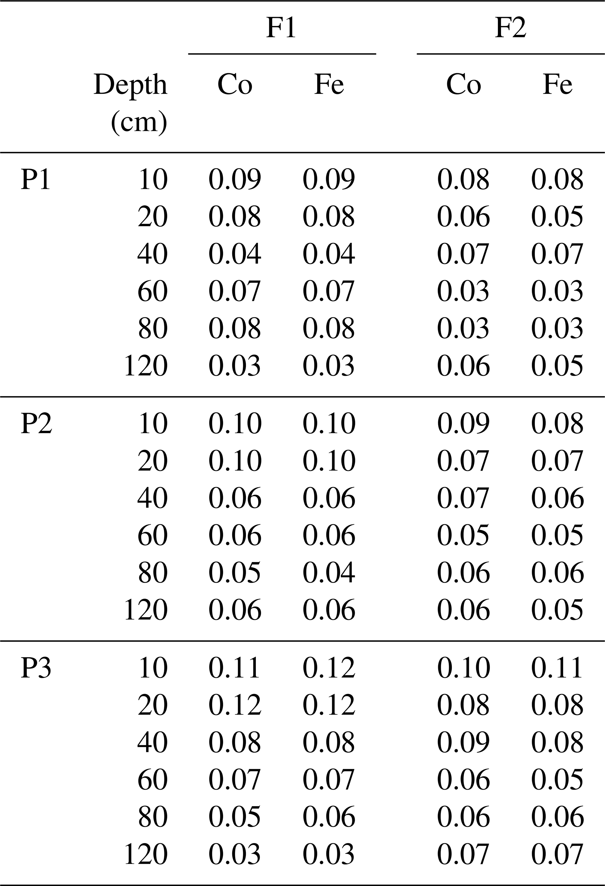
Soil water content and soil water potential were measured hourly by homemade time domain reflectometer (TDR) probes (Cai et al., 2016), tensiometers (T4e, UMS GmbH), and dielectric water potential sensors (MPS-2 matric potential and temperature sensor, Decagon Devices), respectively. Sensors were installed at 10, 20, 40, 60, 80, and 120 cm depth. Root measurements were taken with a digital camera (Bartz Technology Corporation) repeatedly from both left and right sides at 20 locations along horizontally installed minirhizotubes 7 m long (clear acrylic glass tubes with outer and inner diameters of 64 and 56 mm, respectively). The calibration of the sensors, root growth observation, and post-processing of the data were described in detail in Cai et al. (2016, 2017).

2.2.2 Sap flow, leaf water hydraulic head, and gas fluxes measurement

Five, three, and five sap flow sensors (SAG3; Dynamax Inc., Houston, USA) were installed in the irrigated, rainfed, and sheltered treatments, respectively, at the beginning of wheat anthesis when stem diameters ranged between 3 and 5 mm. Vertical and horizontal temperature gradients (dT) of each sensor were recorded at 10 min intervals with a CR1000 data logger and two AM 16∕32 multiplexers (Campbell Scientific, Logan, Utah). Sensor heat inputs were controlled by voltage regulators controlled by the CR1000 data logger. The raw signal data were aggregated to 30 min intervals, and sap flow was calculated following Langensiepen et al. (2014). The number of tillers per square meter was counted every 2 weeks during the operation period of sap flow sensors (26 May–23 July 2016). Tiller numbers were used to upscale the sap flow of single tiller (g h⁻¹) to canopy transpiration rate (mm h⁻¹ or mm d⁻¹).

Leaf stomatal conductance and the leaf water hydraulic head were measured every 2 weeks from 07:00 to 20:00 LT (local time) under clear and sunny conditions from tillering (20 April) to the beginning of maturation (29 June 2016). The stomatal conductance to water vapor of three to four upmost fully developed leaves was measured using a LICOR 6400 XT device (Licor Biosciences, Lincoln, Nebraska, USA) with a reference CO₂ concentration of 400 ppm and a flow rate of 500 (µmol s⁻¹) and using real-time records of photosynthetic active radiation, vapor pressure deficit, and leaf temperature provided by the instrument. Then the leaves were quickly detached by a sharp knife to measure leaf water pressure head with a digital pressure chamber (SKPM 140/(40-50-80), Skye Instrument Ltd, UK).

Plant hydraulic conductance in crop species can be estimated by measuring the transpiration and the root zone and leaf water hydraulic heads (Tsuda and Tyree, 1997). In our study, we calculated the conductance according to Ohm's law by dividing the hourly sap flow by the difference between effective root zone hydraulic head and leaf hydraulic head. The effective root zone hydraulic head was calculated based on hourly measured soil water hydraulic head and measured root length density (cm cm⁻²) at six depths (10, 20, 40, 60, 80, and 120 cm) in the soil profile following Eqs. (8) and (10) (see Sect. 2.3.4). During one measurement day, six hourly values of the conductance were obtained from measurements between 11:00 and 16:00 LT. The average and standard deviation of these hourly measurements were calculated for each measurement day. However, the hydraulic conductance can vary within short time periods due to the role of aquaporins (Maurel et al., 2008; Javot and Maurel, 2002; Henzler et al., 1999) or abscisic acid (ABA) regulation (Parent et al., 2009) and xylem cavitation (Sperry et al., 2003). We assumed however a constant plant hydraulic conductance during the day.

Canopy gas exchange was measured hourly on the same days when leaf water pressure heads were measured with a closed chamber system (Langensiepen et al., 2012). CO₂ concentration was derived with a regression approach by Langensiepen et al. (2012). Because we were interested in comparing measured with calculated hourly instantaneous gross assimilation by the newly coupled root–shoot model (LINTULCC2 with other subroutines), the total soil respiration (i.e., heterotrophic organisms and root respiration) was subtracted from the instantaneous canopy CO₂ exchange rate measured by the closed chamber. The total soil respiration was calculated based on measured soil temperature, soil water content at 10 cm soil depth, and leaf area index from crops using the fitted parameters derived from the same field and soil types (Prolingheuer et al., 2010). The calculated total soil respiration was compared and validated with the measured values in the same field in the previous years from Stadler et al. (2015).

2.2.3 Crop growth

Crop growth information was collected biweekly from 20 April until harvest on 26 July 2016. Leaf area index and crop biomass were measured by harvests of two rows (1 m each) for each treatment. Leaves were separated into green leaves and brown leaves, and the brown and green leaf area was measured using a leaf area meter (LI-3100C, Licor Biosciences, and Lincoln, Nebraska, USA). The aboveground biomass was measured using the oven drying method. Samples were first weighed in total, then separated into different plant organs (green leaf, brown leaf, stem, ear, and grain) and weighed. Subsamples were extracted afterward from these samples, weighed, dried in an oven at 105 ^∘C for 48 h, and weighed again for determining dry matter. At the end of the growing season, four replicates of 1 m² of plants were harvested from the plots to determine grain yield and harvest index.

2.3 Model description

2.3.1 Description of the original LINTULCC crop model

We used the crop model LINTULCC2 (Rodriguez et al., 2001). LINTULCC2 couples photosynthesis to stomatal conductance and can perform a detailed calculation of leaf energy balances (Rodriguez et al., 2001; see Appendix A). This model was validated and compared with different crop models for spring wheat and used to simulate the effects of elevated CO₂ and drought conditions (Ewert et al., 2002; Rodriguez et al., 2001). LINTULCC2 calculates phenology, leaf growth, assimilate partitioning, and root growth following the procedure outlined in Rodriguez et al. (2001).

In LINTULCC2, the assimilation rate of the sunlit and shaded leaf is calculated using the biochemical model of Farquhar and von Caemmerer (1982). Stomatal conductance (g_s) was calculated according to the model Leuning (1995) for sunlit and shaded leaves separately. In LINTULCC2 CO₂ uptake is calculated as a function of CO₂ demand by photosynthesis and the ambient concentration of CO₂, using the iterative methodology proposed by Leuning (1995) (Appendix A). For the sake of simplification, in LINTULCC2, the internal leaf CO₂ concentration, C_i, is initially assumed to be 0.7 times the atmospheric CO₂ concentration C_a (Vico and Porporato, 2008; Rodriguez et al., 2001; Jones, 1992). Then, the light-saturated photosynthetic rate of sunlit and shaded leaves (AMAXsun and AMAXshade; µM CO₂ m⁻² s⁻¹) and the quantum yield for sunlit and shaded leaves (EFFsun and EFFshade; µM CO₂ MJ⁻¹) are calculated iteratively (Farquhar et al., 1980; Farquhar and von Caemmerer, 1982). This iterative loop ends when the difference in calculated internal CO₂ mole fraction between two consecutive loops is <0.1 µmol mol⁻¹ (Appendix A). Based on a fraction of sunlit (and shaded) leaf area and leaf area index (LAI), the leaf stomatal resistance of sunlit and shaded leaves was integrated over the canopy leaf area to the canopy resistance (r_s) (Appendix B).

The canopy resistance, crop height, and calculated crop albedo (depending on both crop and soil water content of the surface layer) and the surface energy balance were used to calculate potential crop evapotranspiration (ETP in mm h⁻¹) using the Penman–Monteith equation (Allen et al., 1998; see Appendix B). The obtained potential surface evapotranspiration is then split into evaporation and potential transpiration using

$$\begin{array}{}\text{(1)}& T_{\mathrm{pot}}=\mathrm{ETP}\left(\mathrm{1}-e^{-k\mathrm{LAI}}\right),\end{array}$$

where k is the light extinction coefficient (0.6 in this study; De Faria et al., 1994; Mo and Liu, 2001; Rodriguez et al., 2001).

T_pot (mm h⁻¹) represents by definition the transpiration of the crop that is not limited by the root zone water hydraulic head. In Sect. 2.3.4 it is explained how the actual transpiration, T_plant (mm h⁻¹), is calculated as a function of the potential transpiration and the root zone soil water pressure head. The ratio T_plant∕T_pot defines the water stress factor f_wat, which is used in the photosynthesis model:

$$\begin{array}{}\text{(2)}& f_{\mathrm{wat}}={\displaystyle \frac{T_{\mathrm{plant}}}{T_{\mathrm{pot}}}}.\end{array}$$

Originally, LINTULCC2 runs at daily time steps (which allows for the within-day variations in temperature, radiation, and vapor pressure deficit). LINTULCC2 requires daily maximum and minimum temperature, actual vapor pressure, rainfall, wind speed, and global radiation. In order to capture the diurnal response of stomata, we modified the time step of the photosynthesis and stomatal conductance subroutine from daily to hourly, while daily time steps were kept in the remaining subroutines (phenology, leaf growth, and biomass partition).

2.3.2 Root growth model

Root growth was simulated using SLIMROOT (Addiscott and Whitmore, 1991). The vertical extension of the seminal roots and the distribution of the lateral roots within the soil profile depend on the root biomass, the soil bulk density, the soil water content calculated by HILLFLOW 1D (Bronstert and Plate, 1997), and the soil temperature computed by STMPsim (Williams and Izaurralde, 2005). The supply of assimilates from the shoot (RWRT; g m⁻² d⁻¹) is given by a partitioning table based on the thermal time (van Laar et al., 1997) that is used to calculate the vertical penetration of seminal and lateral roots. The assimilate allocation for seminal root growth (ASROOT) is constrained by daily supply of assimilates from the shoot RWRT (g m⁻² d⁻¹) and the demand of assimilates from seminal roots (ASROOT_demand).

$$\begin{array}{}\text{(3)}& \mathrm{ASROOT}=\min \left({\mathrm{ASROOT}}_{\mathrm{demand}},\mathrm{RWRT}\right)\end{array}$$

ASROOT_demand is a function of the number of seminal roots per square meter (NSROOT), which depends on the number of emerged plants per square meter and the number of seminal roots per plant, the specific weight of seminal roots WSROOT (g m⁻¹), and the daily elongation rate of seminal roots RSROOT (m d⁻¹):

$$\begin{array}{}\text{(4)}& {\mathrm{ASROOT}}_{\mathrm{demand}}=\mathrm{RSROOT}\cdot \mathrm{WSROOT}\cdot \mathrm{NSROOT}.\end{array}$$

RSROOT depends on the soil temperature and is constrained by a maximal elongation rate, RSROOT_max, and the soil-temperature-dependent rate, which is an empirical function of the soil temperature of the deepest layer where roots are growing, TBOTLAYER (K) (Jamieson and Ewert, 1999):

$$\begin{array}{}\text{(5)}& \mathrm{RSROOT}=\min \left({\mathrm{RSROOT}}_{\max },\mathrm{TBOTLAYER}\cdot \mathrm{RTFAC}\right),\end{array}$$

where RTFAC is the temperature factor driving the penetration of seminal roots (m K⁻¹ d⁻¹) and TBOTLAYER (K) the soil temperature of the deepest layer where roots are growing. When soil temperature is below or equal to 0 ^∘C, no seminal growth occurs. The maximum daily elongation rate of seminal roots, RSROOT_max, was set at 0.03 m d⁻¹ for wheat according to Watt et al. (2006).

The daily increment in seminal root length (SRLIR; m m⁻² d⁻¹) is defined as

$$\begin{array}{}\text{(6)}& \mathrm{SRLIR}=\mathrm{ASROOT}/\mathrm{WSROOT}.\end{array}$$

Lateral roots are simulated when the root biomass supplied by the shoot is greater than the assimilate demand of seminal roots (RWRT > ASROOT_demand). Lateral root biomass is distributed stepwise from the top layer to the deepest soil layer with seminal roots.

Roots start to die after anthesis. Since the specific weight of the roots of cereal crops varies with soil strength (Colombi et al., 2017; Lipiec et al., 2016; Hernandez-Ramirez et al., 2014; Merotto and Mundstock, 1999), we chose different specific weights for the stony (F1) and silty soil (F2) from the range that was observed by Noordwijk and Brouwer (1991) and Jamieson and Ewert (1999) in soils with different soil strength (Appendix C).

2.3.3 Physically based soil water balance model

HILLFLOW 1D was chosen for calculating the water pressure heads in the soil and how they change with depth and time as a function of the precipitation, soil evaporation, RWU, and water percolation at the bottom of the simulated soil profile (Bronstert and Plate, 1997). HILLFLOW 1D calculates soil water content and water fluxes by numerically solving the Darcy equation for unsaturated water flow in porous media (Bronstert and Plate, 1997). The relations between soil water hydraulic head, water content, and hydraulic conductivity are described by the Mualem–van Genuchten functions (van Genuchten, 1980). The parameters of these functions, i.e., the soil hydraulic parameters, for the different soil layers and the two sites were taken from Cai et al. (2018) (Appendix D). In this study, a soil depth of 1.5 m vertically discretized into 50 layers was considered. A free drainage bottom boundary and a mixed flux-matric potential boundary at the soil surface were implemented. The mixed upper boundary condition prescribes the flux at the soil surface by the precipitation and evaporation rates as long as the soil water pressure heads are not above or below critical heads. When these heads are reached, the boundary conditions are switched to constant pressure head boundary conditions.

2.3.4 Feddes' and Couvreur's root water uptake models

The Feddes RWU model (Feddes et al., 1978; see Appendix E) was already built in the HILLFLOW 1D model (Bronstert and Plate, 1997). We implemented the Couvreur RWU model (Couvreur et al., 2012, 2014) into HILLFLOW. In both models, T_plant is calculated from the sum of the simulated RWU in the different soil layers and used to calculate the water stress factor (f_wat) following Eq. (2), which was used in the photosynthesis model. In the Feddes model, root water uptake from a soil layer is proportional to the normalized root density, NRLD (m⁻¹), in that layer and is multiplied by a stress function α that depends on the soil water pressure head, ψ_m (m), in that soil layer and the potential transpiration rate (see Appendix E for the definition of α):

$$\begin{array}{}\text{(7)}& {\mathrm{RWU}}_i=\mathit{\alpha }\left({\mathit{\psi }}_{m,i},T_{\mathrm{pot}}\right)T_{\mathrm{pot}}{\mathrm{NRLD}}_i\mathrm{\Delta }{z}_i,\end{array}$$

where NRLD_i is calculated from the root length density, RLD (m m⁻³), and discretized soil dept, Δz_i (m), as

$$\begin{array}{}\text{(8)}& {\mathrm{NRLD}}_i={\mathrm{RLD}}_i/\sum _{i=\mathrm{1}}^N{\mathrm{RLD}}_i\mathrm{\Delta }{z}_i.\end{array}$$

The parameters of the α stress functions model were taken from Cai et al. (2018; see Appendix C). According to Eq. (7), the reduction of water uptake in a given layer depends on the soil water pressure head in that layer only and does not influence the water uptake in other layers. This means that a reduced water uptake in dried out soil layers directly leads to a reduction of the total root water uptake and plant transpiration and is not compensated by increased uptake in other layers where there is still water available.

In the Couvreur model, the root water uptake in a given soil layer is related to the water potentials in the root system and root water uptake in other soil layers so that compensatory uptake is considered in this model. Root water uptake in a certain layer is obtained from

$$\begin{array}{}\text{(9)}& {\mathrm{RWU}}_i=T_{\mathrm{plant}}{\mathrm{NRLD}}_i\mathrm{\Delta }{z}_i+K_{\mathrm{comp}}\left({\mathit{\psi }}_i-{\mathit{\psi }}_{s_{\mathrm{r}}}\right){\mathrm{NRLD}}_i\mathrm{\Delta }{z}_i,\end{array}$$

where ψ_i (m) is the total hydraulic head (or hydraulic head which is the sum of the pressure head and gravitation potential heads) in layer i, ${\mathit{\psi }}_{s_{\mathrm{r}}}$ (m) is the average hydraulic head in the root zone, and K_comp (d⁻¹) is the root system conductance for compensatory uptake. The first term of Eq. (9) represents the uptake from that soil layer when the hydraulic head is uniform in the root zone, and the second term represents the increase or decrease of uptake from the soil layer due to a respectively higher and lower hydraulic head in layer i than the average hydraulic head. The average root zone hydraulic head is calculated as the weighted average of the hydraulic heads in the different soil layers as

$$\begin{array}{}\text{(10)}& {\mathit{\psi }}_{s_{\mathrm{r}}}=\sum _{i=\mathrm{1}}^N{\mathit{\psi }}_i{\mathrm{NRLD}}_i\mathrm{\Delta }{z}_i.\end{array}$$

The plant transpiration rate is the minimum of the potential transpiration rate and the transpiration rate, T_threshold (mm h⁻¹), when the hydraulic head in the leaves reaches a threshold value, ψ_threshold (m), that triggers stomatal closure:

$$\begin{array}{}\text{(11)}& T_{\mathrm{plant}}=\max \left(\mathrm{0},\min \left(T_{\mathrm{pot}},T_{\mathrm{threshold}}\right)\right).\end{array}$$

T_threshold is calculated from the difference between the root zone hydraulic head and the threshold hydraulic head in the leaves ψ_threshold that is multiplied by the plant hydraulic conductance, K_plant as

$$\begin{array}{}\text{(12)}& T_{\mathrm{threshold}}=K_{\mathrm{plant}}\left({\mathit{\psi }}_{s_{\mathrm{r}}}-{\mathit{\psi }}_{\mathrm{threshold}}\right).\end{array}$$

In our study, we used the critical leaf hydraulic head, ψ_threshold, of −200 m (equivalent to −2 MPa) (Cochard, 2002; Tardieu and Simonneau, 1998). The original Couvreur model only considers the hydraulic conductance from the roots to the plant collar, $K_{r_{\mathrm{s}}}$, by assuming that the hydraulic resistance from plant collar to leaves is minor as compared to root system resistance. The shoot hydraulic resistance could be large in some crop plants (Gallardo et al., 1996) or in trees (Domec and Pruyn, 2008; Tsuda and Tyree, 1997). In order to simulate the leaf water hydraulic head, the whole plant hydraulic conductance (K_plant) needs to be used. The whole plant hydraulic conductance could be estimated from different components (i.e., soil to roots, stem to leaf) following an approach from Saliendra et al. (1995) or a more complex attempt by Janott et al. (2011). Because hydraulic data from plant collar to leaf are rare and difficult to obtain and account for differing species characteristics and environmental conditions, for the sake of simplification, we derived K_plant (d⁻¹) from the root hydraulic conductance ($K_{r_{\mathrm{s}},\mathrm{doy}}$), assuming that K_plant is a constant fraction β of $K_{r_{\mathrm{s}},\mathrm{doy}}$ (d⁻¹):

$$\begin{array}{}\text{(13)}& K_{\mathrm{plant}}=\mathit{\beta }{K}_{r_{\mathrm{s}},\mathrm{doy}}.\end{array}$$

We used the measured plant hydraulic conductance from sap flow, leaf water hydraulic head, soil water pressure head, and root observation (Sect. 2.2.1 above) in the lower rainfed plot to calibrate β, which was then applied for all plots (Appendix C). K_plant and $K_{r_{\mathrm{s}}}$ in anisohydric wheat are influenced by soil water availability and crop development. We followed the approach of Cai et al. (2017) to estimate the root hydraulic conductance ($K_{r_{\mathrm{s}},\mathrm{doy}}$) and compensatory root water uptake (K_comp) based on the total length of the root system below a unit surface area, TRLD_doy (m m⁻²), at a given day of year (DOY) (Eq. 14), which is the output from SLIMROOT:

$$\begin{array}{}\text{(14)}& {\mathrm{TRLD}}_{\mathrm{doy}}=\sum _i^N{\mathrm{RLD}}_{i,\mathrm{doy}}\mathrm{\Delta }{z}_i.\end{array}$$

Assuming the same conductance for all root segments, the root system conductance scales with the TRLD:

$$\begin{array}{}\text{(15)}& K_{r_{\mathrm{s}},\mathrm{doy}}=K_{r_{\mathrm{s}},\mathrm{normalized}}{\mathrm{TRLD}}_{\mathrm{doy}},\end{array}$$

where $K_{r_{\mathrm{s}},\mathrm{normalized}}$ (d⁻¹ cm⁻¹ cm²) is the root system conductance per unit root length per surface area. For $K_{r_{\mathrm{s}},\mathrm{normalized}}$, we took the average value that was obtained by Cai et al. (2018) for the stony soil (F1) and silty soil (F2) sites: $\mathrm{0.2544}\times {\mathrm{10}}^{-\mathrm{5}}$ (cm d⁻¹) (Appendix C).

Many studies included hydraulic conductance along the soil–plant–atmosphere pathway to simulate water transport (Verhoef and Egea, 2014; Wang et al., 2007; Tuzet et al., 2003; Olioso et al., 1996). However, both root and plant hydraulic conductance in these studies were assumed constant. In our work, the plant hydraulic conductance varied following the shoot and root development in the growing season.

2.3.5 Coupling of water balance and root water uptake models with the crop model

We carried out a comprehensive comparison of the following modeling approaches for simulating CO₂ and H₂O fluxes and crop growth (Fig. 2):

• HILLFLOW 1D–Couvreur's RWU–SLIMROOT–LINTULCC2 (Co)

• HILLFLOW 1D–Feddes' RWU–SLIMROOT–LINTULCC2 (Fe).

The photosynthesis and stomatal conductance subroutines, RWU and HILLFLOW 1D water balance model, and evaporative demand (ETP) were run or specified with hourly time steps, while phenology, leaf growth, root growth, and biomass partitioning were updated daily. For a certain hourly time step $\mathrm{\Delta }{t}_i=t_i-t_{i-\mathrm{1}}$, different modules were solved in the following sequence. First, LINTULCC2 was used with a water stress factor f_wat=1 to calculate the leaf and canopy resistance and the potential transpiration rate. T_pot was then used in HILLFLOW 1D to calculate the soil water pressure head changes, water content changes, the actual transpiration, and f_wat during the time step. LINTULCC2 was then run again using f_wat. The leaf conductance and assimilation rate were calculated. For the next time step, the same loop was run, and hourly assimilation was accumulated to a daily value. Daily assimilation rates were used in modules that run with a daily time step, for instance, modules of LINTLCC2 that calculate assimilate partitioning which is used to calculate shoot (LAI) development and passed to SLIMROOT to simulate root development (Fig. 2). Before comparing these modeling approaches, we calibrated the original LINTULCC model using the data from the rainfed plots in the silty soil (F2P2). The model is firstly calibrated to make sure the model properly described the phenology. Two parameters (minimum thermal sum from sowing to anthesis and thermal sum from anthesis to maturity; ^∘C d) were used for phenology calibration based on information of sowing, anthesis, and maturity dates. The model was then calibrated using time series of LAI, biomass, and gross assimilation rate through the change of maximum carboxylation rate at 25 ^∘C (VCMAX25), critical leaf area index (LAICR), and relative growth rate of leaf area during exponential growth (RGRL) parameters. The same crop parameters and soil parameters were applied for both model configurations (Appendices C and D). All presented flux data (soil water flux, gross assimilation rate, sap flow, stomatal conductance, and leaf water pressure head) and the simulated outputs were converted from local time to coordinated universal time (UTC) to avoid the confusion in interpretation.

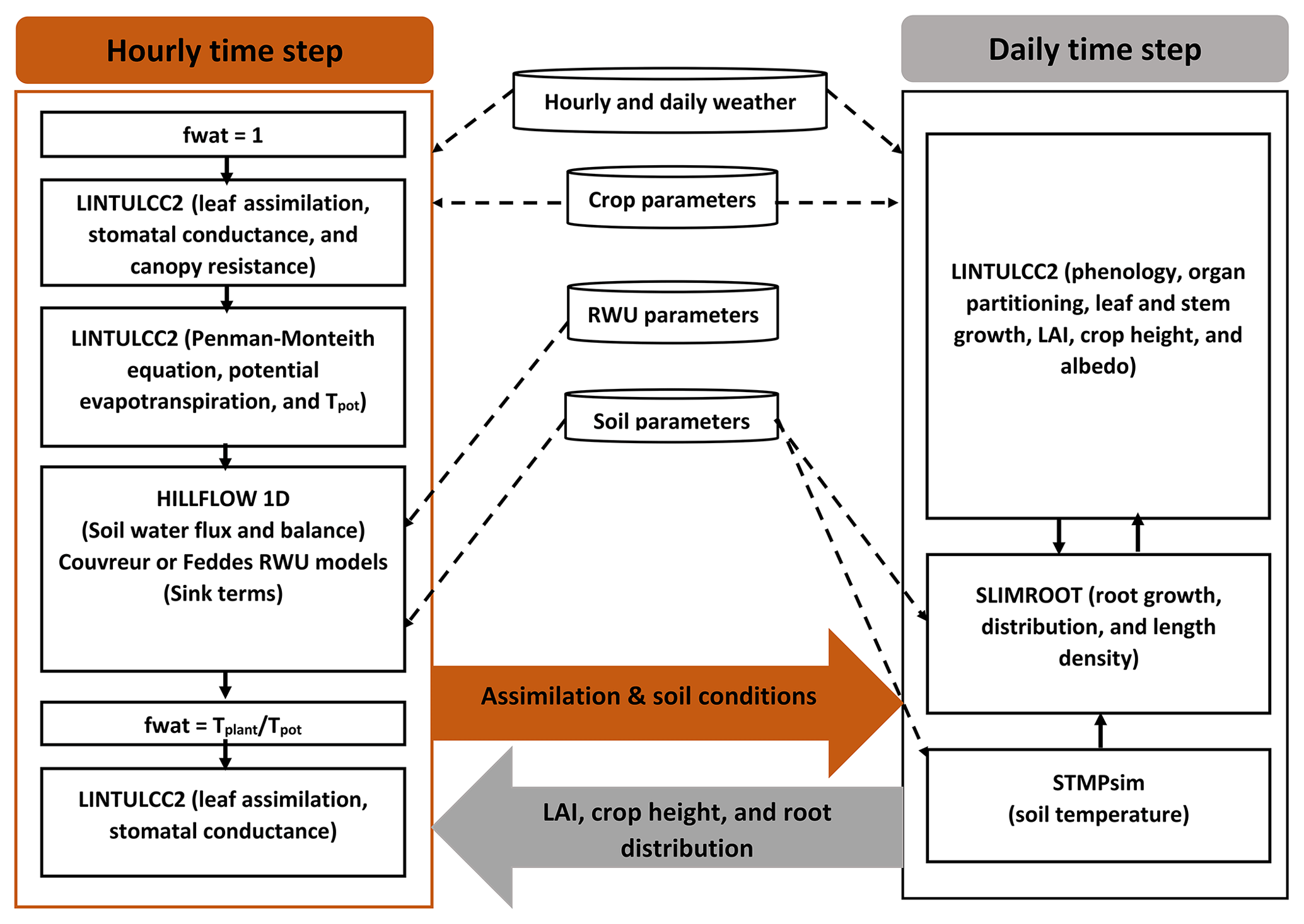
Figure 2 Description of the coupled root–shoot models in the study. The orange arrow indicates feedbacks from the hourly simulations to daily simulation, while the grey arrow indicates feedbacks from the daily simulations to the hourly simulations. The dashed black arrows denote the weather input and parameters to the subroutines. The continuous black arrows indicate the links amongst the modeling subroutines.

2.4 Criteria for model comparison and evaluation

We analyzed the performance of two modeling approaches following the approach from Willmott (1981): (i) correlation coefficient (r) (Eq. 16); (ii) the degree to which simulated values approached the observations or index of agreement (I) defined in Eq. (17), varying from 1 (for perfect agreement) to 0 (for no agreement); (iii) the root mean square error (RMSE), computed to characterize the difference between simulated values and observed data (Eq. 18):

$$\begin{array}{}\text{(16)}& {\displaystyle }& {\displaystyle }r={\displaystyle \frac{\sum _{i=\mathrm{1}}^n\left({\mathrm{Sim}}_i-\stackrel{\mathrm{‾}}{\mathrm{Sim}}\right)\left({\mathrm{Obs}}_i-\stackrel{\mathrm{‾}}{\mathrm{Obs}}\right)}{\sqrt{\left[\sum _{i=\mathrm{1}}^n{\left({\mathrm{Sim}}_i-\stackrel{\mathrm{‾}}{\mathrm{Sim}}\right)}^{\mathrm{2}}\right]\left[\sum _{i=\mathrm{1}}^n{\left({\mathrm{Obs}}_i-\stackrel{\mathrm{‾}}{\mathrm{Obs}}\right)}^{\mathrm{2}}\right]}}}\text{(17)}& {\displaystyle }& {\displaystyle }I=\mathrm{1}-\left[{\displaystyle \frac{\sum _{i=\mathrm{1}}^n{\left({\mathrm{Sim}}_i-{\mathrm{Obs}}_i\right)}^{\mathrm{2}}}{\sum _{i=\mathrm{1}}^n{\left(\left|{\mathrm{Sim}}_i-\stackrel{\mathrm{‾}}{\mathrm{Obs}}\right|+\mathrm{|}{\mathrm{Obs}}_i-\stackrel{\mathrm{‾}}{\mathrm{Obs}}\mathrm{|}\right)}^{\mathrm{2}}}}\right]\text{(18)}& {\displaystyle }& {\displaystyle }\mathrm{RMSE}=\sqrt{{\displaystyle \frac{\sum _{i=\mathrm{1}}^n{\left({\mathrm{Sim}}_i-{\mathrm{Obs}}_i\right)}^{\mathrm{2}}}{n}}},\end{array}$$

where Sim and Obs are simulated and measured variables; i is the index of a given variable; $\stackrel{\mathrm{‾}}{\mathrm{Obs}}$ and $\stackrel{\mathrm{‾}}{\mathrm{Sim}}$ are the mean of the simulated and measured data; and n is the number of observations.

2.5 Sensitivity analysis

The parameters of the SLIMROOT root growth model and the Couvreur RWU model were derived from literature data. However, these parameters are uncertain and vary between different wheat varieties. In order to evaluate the effect of these parameters on the simulated crop growth and root water uptake, we carried out a sensitivity analysis.

In a first set of simulations, the root length normalized root system conductivity $K_{r_{\mathrm{s}},\mathrm{normalized}}$ was varied from 0.1 to 40 times the $K_{r_{\mathrm{s}},\mathrm{normalized}}=\mathrm{0.2554}\times {\mathrm{10}}^{-\mathrm{5}}$ cm d⁻¹ that was estimated by Cai et al. (2018). The root system hydraulic conductance is related to the total root length, which depends on the specific weight of lateral and seminal roots. These two parameters are rarely reported, especially for field-grown wheat (Noordwijk and Brouwer, 1991). The observed specific weight of lateral roots in wheat was reported to be in the range of 0.00406 to 0.00613 g m⁻¹ (Noordwijk and Brouwer, 1991). Huang et al. (1991) found that the specific weight of seminal roots of winter wheat grown under controlled soil chamber conditions decreased from 0.023 to 0.0052 g m⁻¹ when air temperature increased from 10 to 30 ^∘C. The values of 0.015 and 0.0035 g m⁻¹ are often used for specific weights of seminal and lateral roots, respectively, in crop growth simulations of wheat cultivars (Mboh et al., 2019; Jamieson and Ewert, 1999). In a second set of simulations, the specific weight of lateral roots was changed from 0.002, 0.003, 0.0035, 0.004, 0.005, 0.006, and 0.007 g m⁻¹, while the specific weight of seminal roots was the same (0.015 g m⁻¹) for all simulations. For the third set of simulations, the specific weight of lateral roots was kept at 0.0035 g m⁻¹, while the specific weight of seminal roots varied from 0.005, 0.0075, 0.01, 0.0125, 0.015, 0.0175, 0.02, and 0.0225 g m⁻¹. In the last sensitivity exercise, the critical leaf hydraulic head threshold (ψ_threshold) was varied between −120 and −260 m.

3 Results and discussion

In the first section, we discuss the performance of the two coupled root–shoot models with the Couvreur RWU model (Co model) and Feddes RWU model (Fe model). The comparative analysis firstly focuses on simulating crop growth and root development under different water conditions and soil types. Next, the simulated transpiration reduction, soil water dynamics, RWU, and gross assimilation rate are presented and discussed. The K_plant is explicitly simulated by the Co model in the different soils and treatments and is compared with direct estimates of K_plant from measurements. In the second part, we discuss the sensitivity analysis of the Co model to understand the effects of changing $K_{r_{\mathrm{s}},\mathrm{normalized}}$, the specific weight of seminal and lateral roots, and Ψ_threshold on the simulated biomass growth and RWU in different soils and under different water regimes.

Figure 3 Comparison between observed (cyan dot) and simulated (a) aboveground dry matter and (b) LAI by Couvreur (Co; solid red line) and Feddes (Fe; solid blue line) model in the sheltered (P1), rainfed (P2), and irrigated (P3) plots of the stony soil (F1) and the silty soil (F2). Note that crop germination was on 26 October 2015; data are shown here from 1 January to harvest on 23 July 2016. RMSE in (a) is kg m⁻² while RMSE in (b) is unitless.

3.1 Comparison of Couvreur's and Feddes' RWU model

3.1.1 Root and shoot (biomass and LAI) growth

Figure 3 shows the dry matter and LAI simulated by the Co and Fe model versus the measured data. The difference between the two samples of the two different rows for each sampling day indicated the heterogeneity in crop growth, even within a small treatment plot. Biomass and LAI simulated by the Co and Fe models were in fair agreement with observations. The r² values of the Co and Fe models were 0.91 and 0.86, respectively, for biomass, while they were 0.76 and 0.75, respectively, for LAI (Table 1). However, both models overestimated dry matter and LAI production in the irrigated and rainfed stony plots, whereas biomass and LAI were underestimated in the sheltered silty plot. This suggests that water stress in the sheltered silty plot was overestimated. For the irrigated stony soil plot, in which the water content stayed high due to the frequent rainfall events and the additional irrigation, it is unlikely that the lower growth is due to water stress. The later start of the growth after the winter could be due to the effects of soil strength and lower soil temperature on crop development in the stony field that were not captured by the model. Soil hardness could constrain root growth while the higher stone content possibly resulted in slower warming up of the soil in spring than the silty soil which in turn slowed down root and crop development.

Table 1 Quantitative and statistical measures of the comparison between two modeling approaches and the observed data for the three water treatments and two soil types. RMSE is the root mean square error; r² is the correlation coefficient; I is the agreement index; n samples is the number of samples. Co is the Couvreur RWU model, and Fe is the Feddes RWU model.

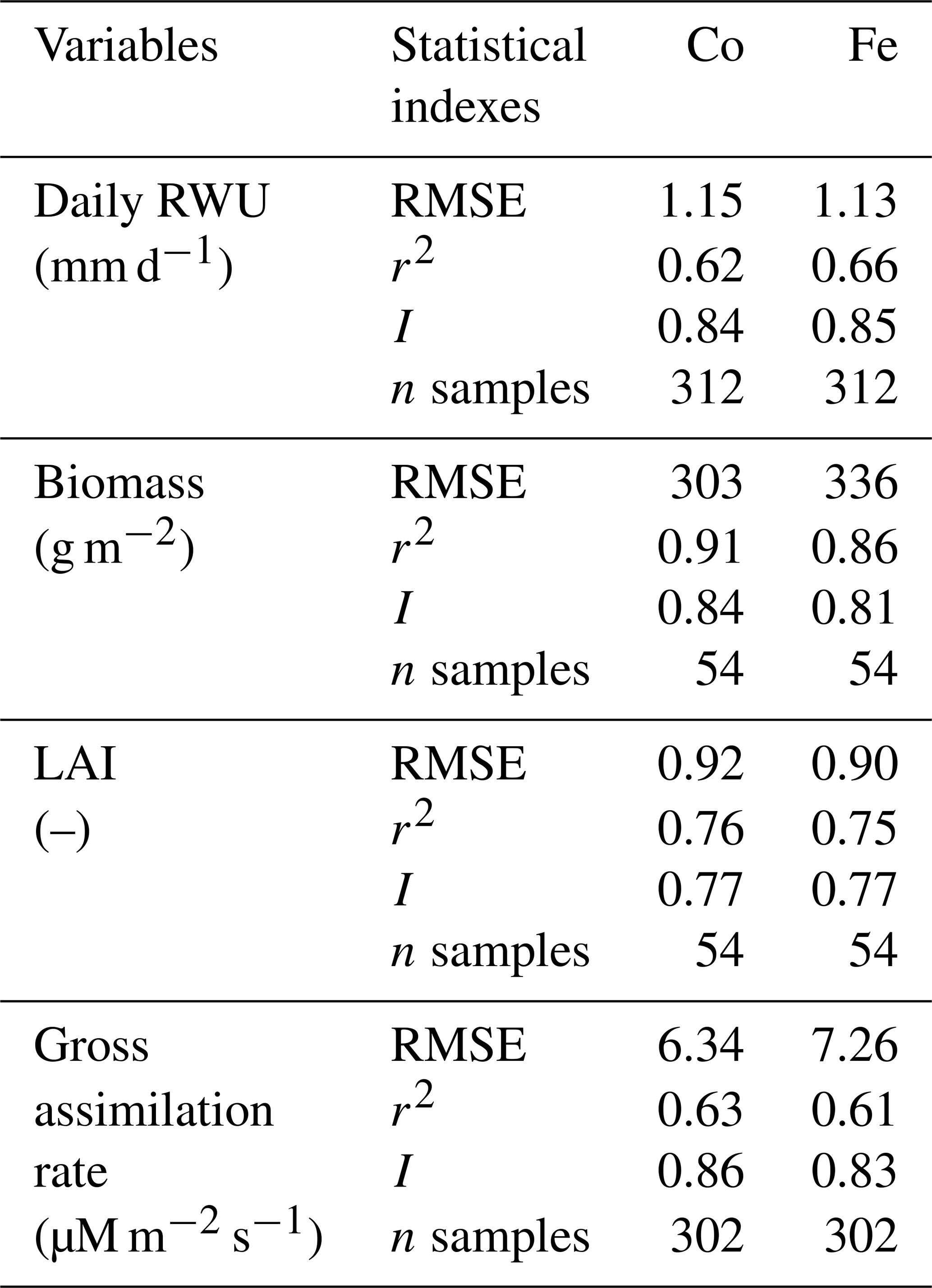
For the stony plots, the Fe and Co models gave similar results, whereas for the silty soil, the Co model reproduced the biomass and LAI better than the Fe model. Although the statistical parameters (r² and RMSE) for the silty soil plots show only a slightly better fit of the Co than of the Fe model, there is a remarkable qualitative difference between the models. The Fe model simulated lower biomass and leaf area in the silty soil than in the stony soil, which is opposite to the observations. The Co model simulated similar biomass and LAI in the irrigated and rainfed plots of the silty and stony soils and higher biomass and LAI in the sheltered plot in silty soil than in the stony soil, which is in closer agreement with the observed differences in biomass and LAI between the two soils. The simulated effect of the soil type on the crop growth was qualitatively correct for the Co model but incorrect for the Fe model.

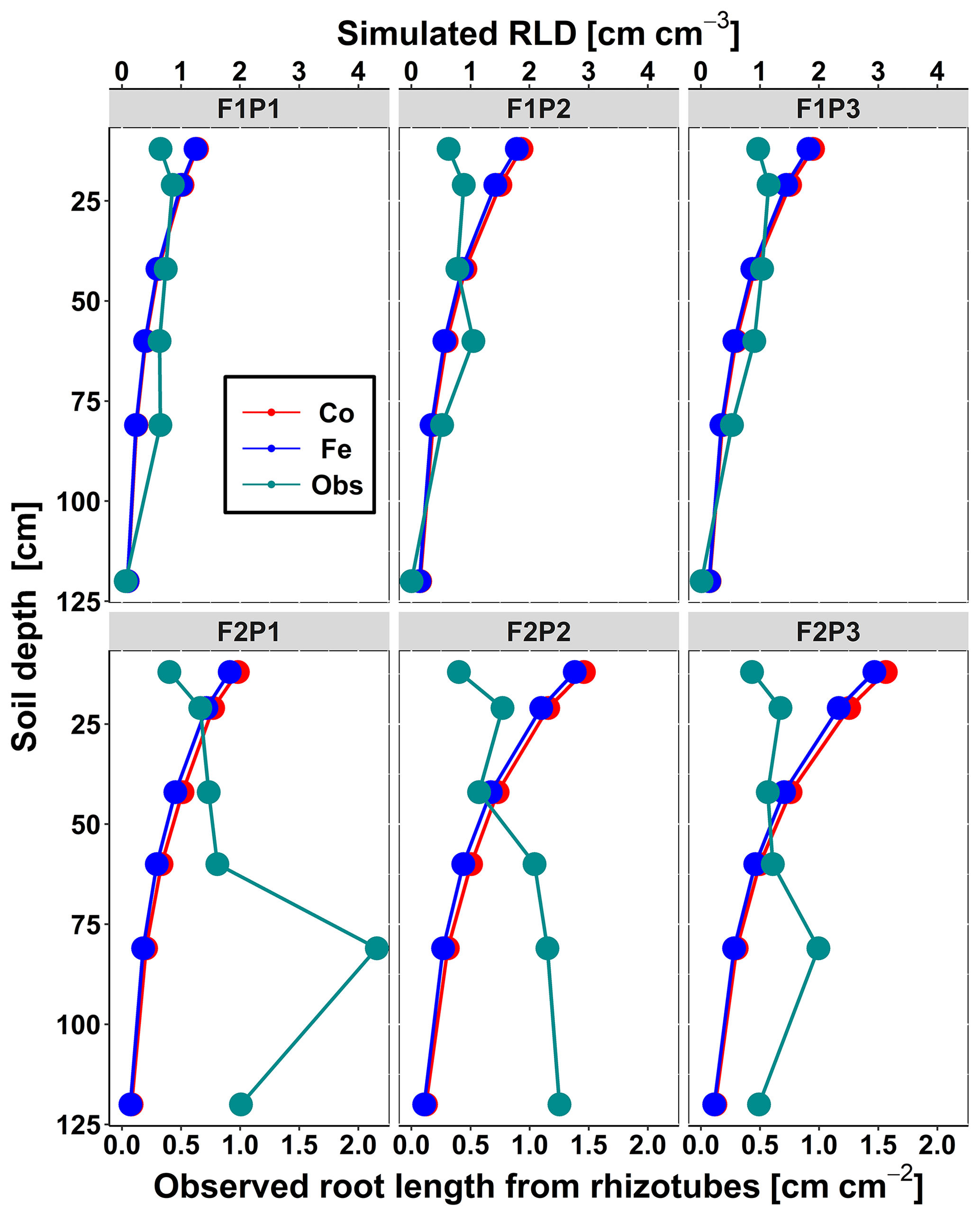
Figure 4 Comparison between observed root length from rhizotubes (cm cm⁻²) (cyan line with dots) and simulated root length density (RLD) (cm cm⁻³) from 10, 20, 40, 60, 80, and 120 cm soil depth at DOY 149 by the Couvreur (Co; solid red) and Feddes (Fe; solid blue) model in the sheltered (P1), rainfed (P2), and irrigated (P3) plots of the stony soil (F1) and the silty soil (F2).

Figure 4 displays the observed root length densities from minirhizotube observations and the simulated ones. Higher root length densities were observed and simulated in the silty soil than in the stony soil. The model simulated smaller root densities in the stony soil because a larger specific weight of the roots was considered for the stony soil than for the silty soil. The simulated root density profiles showed the highest root densities near the surface, whereas the observed profiles, especially in the silty soil, showed higher densities in the deeper soil layers. The model simulated smaller root length densities in the sheltered plots than in the other plots of both the stony and silty soils. This is a consequence of the lower biomass growth that was simulated in the sheltered plots. For the stony soil, this corresponds with the observations that also showed lower root length densities in the sheltered plots than in the other plots. However, for the silty plot, the opposite was observed. For both the simulations and the observations, we compared the ratio of total root lengths in a certain plot and treatment to the total root length in the rainfed stony plot F1P2 (Appendix F). In the stony plots the ratios of the observed total root length to the reference were close to 1, but the simulated total root length in the sheltered plot was smaller than 1. The ratios of the total root lengths in the silty plot to the reference were for all plots larger than 1. Nevertheless, the ratios of observed root lengths were larger (2.27–4.03) than those of the simulated ones (1.04–1.67). The observed ratios were larger for the sheltered plot than for the other plots in the silty soil, whereas the opposite was simulated by the models. Predefined ratios of root and shoot biomass allocation for a given growth period and a source-driven root growth (van Laar et al., 1997) in our models do not allow a shift in carbon allocation to roots (for more root growth) in response to water stress. However, this should not be emphasized too much because the observed imaged root data from minirhizotubes for driving the root length might have potential errors and uncertainties (Cai et al., 2018).

3.1.2 Transpiration reduction, soil water dynamic, RWU, and gross assimilation rate

Figure 5a and b show the reduction of the transpiration compared to the potential transpiration, f_wat, simulated by the Fe and Co models (mid-March until harvest), and Fig. 5c and d show the simulated potential and the simulated and measured actual transpiration rates from the end of April until harvest. The Fe model simulated more water stress than the Co model and a more pronounced and earlier stress in the silty than in the stony soil. As a consequence, the simulated transpiration rates by the Fe model were generally lower than the simulated ones by the Co model. According to the f_wat factors, the Couvreur model also simulated more water stress in the silty soil than in the stony soil. The effect of f_wat on the cumulative transpiration and growth also depends on the timing of the lower f_wat values. At the beginning of the growing season when the LAI and potential transpiration are low, the impact of a lower f_wat on the cumulative transpiration and growth is lower than later in the growing season. These results are in contrast with findings by Cai et al. (2017, 2018), who found that there was no water stress simulated in the silty soil in 2014 by the Co and Fe models. However, the studies from Cai et al. (2018) used the measured root distributions instead of the simulated ones from the root–shoot model. Therefore, in their simulations, the crop had more access to water in the deeper soil layers. Second, they used the Feddes–Jarvis model, which accounts for root water uptake compensation. This could explain why they did not simulate water stress in the silty plot with the Feddes model. Thirdly, weather conditions and irrigation applications were different in their study in 2014 (less dry) from our experimental season in 2016.

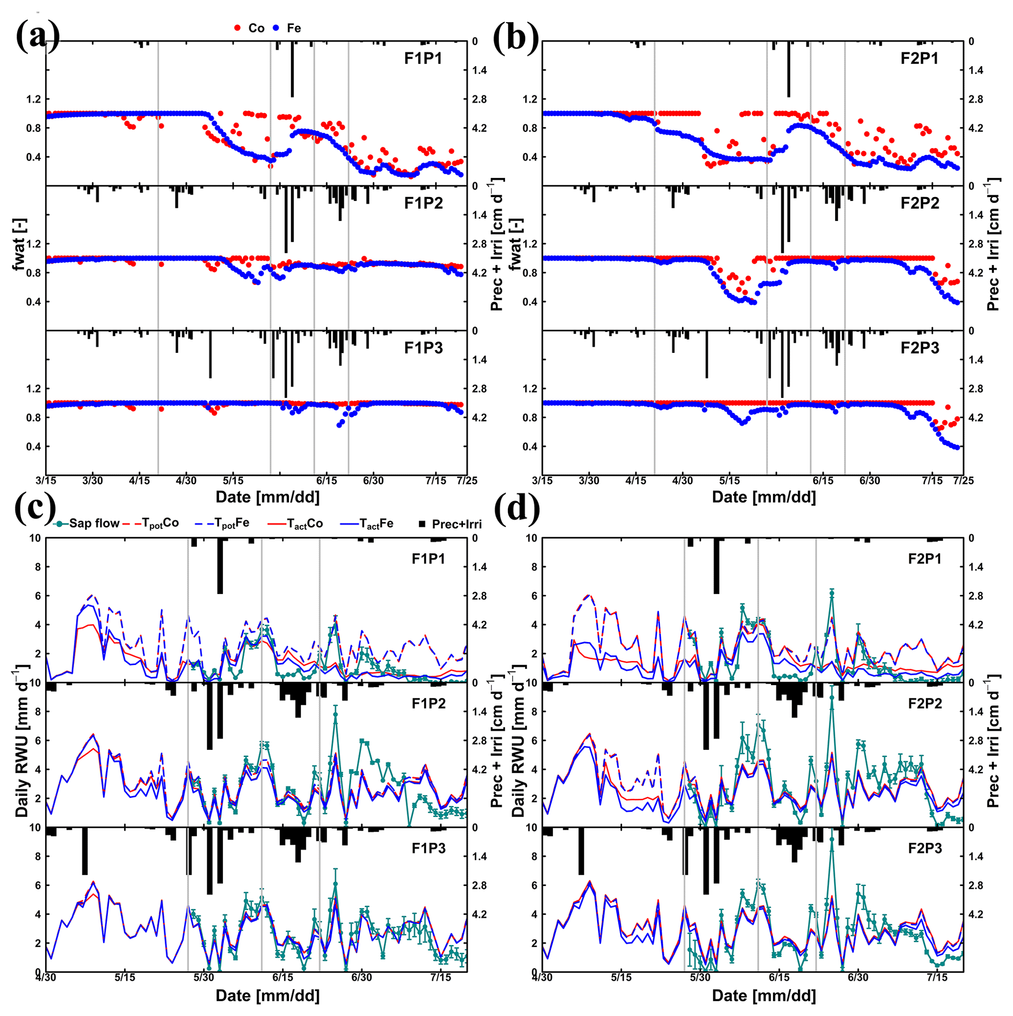
Figure 5 Daily transpiration reduction factor (f_wat) (a, b) from 15 March to harvest on 23 July 2016 and comparison between observed (cyan) and simulated root water uptake (RWU) and potential transpiration simulated (c, d) by the Couvreur (Co; closed red) and Feddes (Fe; closed blue) models from 30 April to 20 July 2016 in the sheltered (P1), rainfed (P2), and irrigated (P3) plots of the stony soil (F1) and the silty soil (F2). Time series of precipitation (Prec) and irrigation (Irri) are given in the panels. Note that crop germination was on 26 October 2015. Vertical cyan bars represent the standard deviation of the flux measurements in the different stems. Vertical grey lines show days with the measured and simulated diurnal courses of root water uptake (RWU), leaf water pressure head (ψ_leaf), stomatal conductance (g_s), and gross assimilation rate (P_g) as used in Fig. 9.

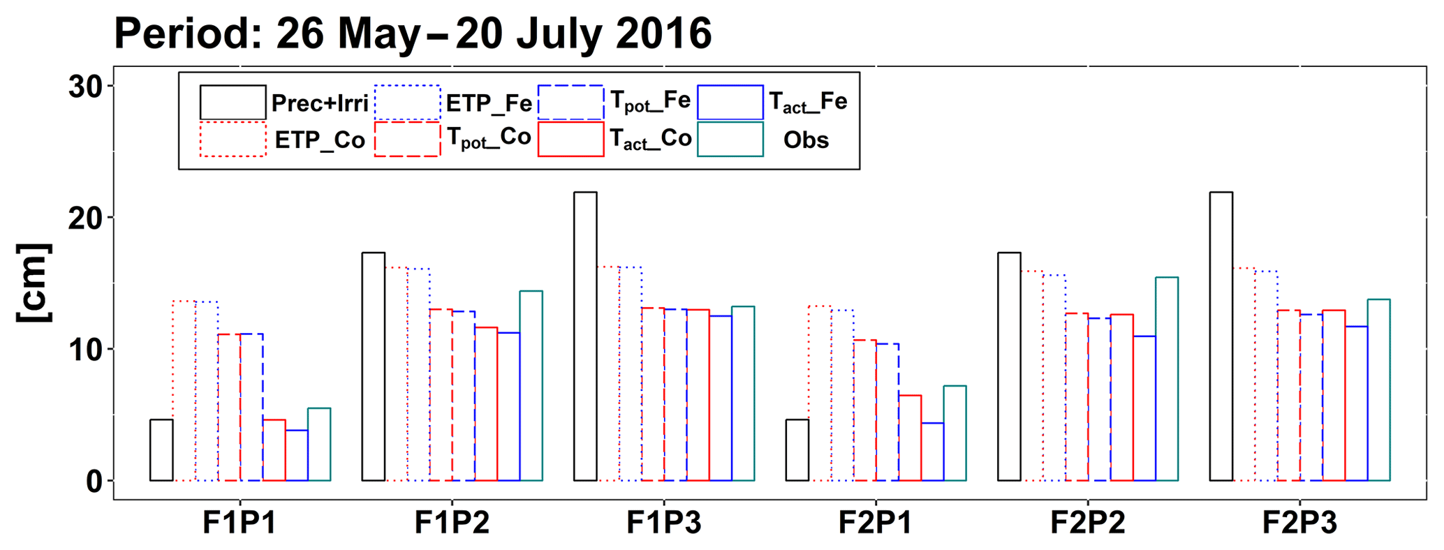
Figure 6 Cumulative precipitation and irrigation (Prec + Irri), potential evapotranspiration (ETP), potential transpiration (T_pot), and actual transpiration (T_act or RWU) simulated by the Couvreur (Co) and Feddes (Fe) models and measured transpiration by sap flow sensors (Obs) from 26 May to 20 July 2016 in the sheltered (P1), rainfed (P2), and irrigated (P3) plots of the stony soil (F1) and the silty soil (F2).

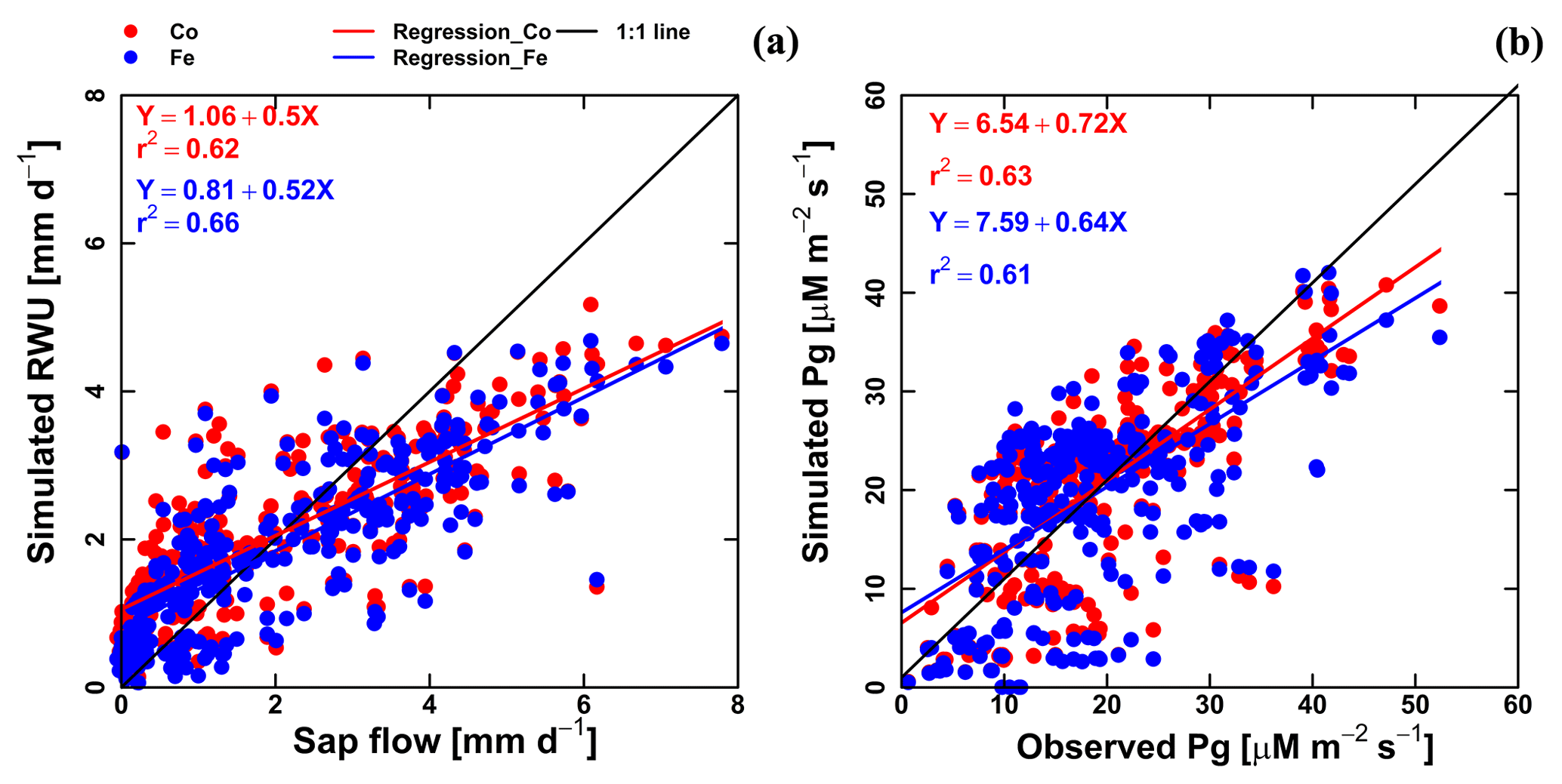
Figure 7 Correlation between observed and simulated (a) daily actual transpiration (or RWU), (b) hourly gross assimilation rate (P_g) from the Couvreur (Co; red dot) and Feddes (Fe; blue dot) models of both fields (F1 and F2). Sap flow data were from 26 May until 20 July 2017 (n=312). Gross assimilation rate from 8 measurement days (n=302). The RMSE in (a) is given in mm d⁻¹, while the RMSE in (b) is given in µM m⁻² s⁻¹.

According to Fig. 5c and d, during the time when sap flow could be measured (from end of May until harvest), the stress factors did not differ a lot between the Fe and Co models. For the rainfed and irrigated plots in the silty soil, the Fe model predicted a stronger reduction in transpiration near the end of the growing season than the Co model. This resulted in a smaller cumulative transpiration predicted by the Fe model than by the Co model over the measurement period in these treatments (Fig. 6). Although this gives the impression that the Co model is better in agreement with the measurements in these treatments, Fig. 5d indicates that this is due to compensating errors. Both models underestimate the measured sap flow in the beginning of the measurement period and overestimate it towards the end, and the Co model overestimates more than the Fe model. This overestimation is due to an overestimation of the LAI by both models near the end of the growing season (Fig. 3b). The reduction of the transpiration in the sheltered plots of the two soils compared to the other treatments is predicted relatively well, but the Fe model predicted more stress and a stronger reduction in transpiration than the Co model, especially in the silty soil. For this treatment, the Co model, which simulated less stress (larger f_wat factors), predicted the cumulative transpiration and how it differed between the two soil types better than the Fe model.

Simulated transpiration in all treatments and both soils are plotted versus the sap flow measurements in Fig. 7. On average, the two models slightly underestimated measured T_act (Fig. 5c and d). This was also found in the study by Cai et al. (2018), in which sap flow was measured in winter wheat in 2014. However, in their study, there was a rather constant offset between the simulations and the sap flow data. One reason could be that in our study we used the simulated LAI values, whereas Cai et al. (2018) used the measured LAI values. In the stony plots, the measured LAIs are overestimated by the simulations so that one would expect an overestimation of the transpiration by the model. The opposite holds true for the silty plot. The overestimation of the LAI at the end of growing season resulted in an overestimation of the transpiration in nonsheltered plots in both soil types. Because of the small size and hollow stem of wheat plants (Langensiepen et al., 2014), it is difficult to install the microsensors and measure the temperature variation for the thin wheat stem with high time frequency under ambient field conditions. In addition, the sap flow in a single tiller is also influenced by spatial variation in environmental conditions. The variability of stem development also results in a significant stem-to-stem variability in sap flow (Cai et al., 2018). The r² values of simulated RWU from the Co and Fe models versus sap flow are 0.62 and 0.66, respectively (Table 1 and Fig. 7a), indicating that our coupled models show a fair performance in the RWU simulation. Measuring gas exchange with closed chamber concentration measurements can significantly alter the microclimatic conditions within the chamber, especially at times of high exchange rate. However using regression functions at the starting point of measurement intervals reduces absolute errors (Langensiepen et al., 2012). The simulated gross assimilation rate (P_g) from two models matched relatively well with the gross assimilation rate measured by a manually closed-canopy chamber, with an r² value of 0.63 and 0.61 for Co and Fe, respectively (Table 1 and Fig. 7b).

The method that we used for modeling the canopy resistance used in the Penman–Monteith equation has been reported for both short and tall crops (Dickinson et al., 1991; Kelliher et al., 1995; Irmak and Mutiibwa, 2010; Perez et al., 2006; Katerji et al., 2011; Srivastava et al., 2018). The fair agreement of RWU to sap flow in our study indicates the proper estimate of ETP based on the crop canopy resistance (with f_wat=1) in winter wheat. The direct calculation of crop canopy resistance in our work allows physiological responses of the crop (stomatal conductance) to solar radiation, temperature, and vapor pressure deficit (Eq. A5) to be captured. In addition, this approach also avoids calculating grass reference evapotranspiration based on a constant canopy resistance.

The differences in simulated stress between the different models were more pronounced in May (Fig. 5) when no sap flow data were available. The Co model predicted less stress and more RWU than the Fe model in May, especially in the rainfed and irrigated plots of the silty soil. The larger stress simulated by the Fe model in the rainfed and irrigated silty plots resulted in a smaller increase in biomass that was simulated in May by the Fe model than by the Co model (Fig. 3a). The measurements of growth in the silty soil do not suggest that there was water stress in these plots in the silty soil, indicating that the Co model better simulated transpiration and growth for these cases than the Fe model. Another way to test the RWU simulated by the different models is to compare the simulated soil water contents (Fig. 8). The Co and Fe models were able to simulate both dynamics and magnitude of soil water content (SWC) in different soil depths and for different water treatments (average of RMSEs over all soil depths was 0.06 for both models; Appendix G). The Co and Fe models displayed lower water contents than the measured ones in the deeper layers at the late growing season (i.e., depth 80 and 120 cm) (Fig. 8). This could be due to the free drainage bottom boundary condition in the HILLFLOW water balance model, which implies that the water can only leave the soil profile, but no water can flow into it from below. Capillary rise in the soil can keep the lower layers relatively wet (Vanderborght et al., 2010). In our simulation, the use of a soil depth of 1.5 m may not be deep enough to capture this effect. The simulated SWC values were however very similar for both models. The larger RWU simulated by the Co than by the Fe model in the silty soil in May resulted in slightly lower simulated water contents by the Co model. But, the differences in simulated water contents by the two models were much smaller than the deviations from the observed water contents.

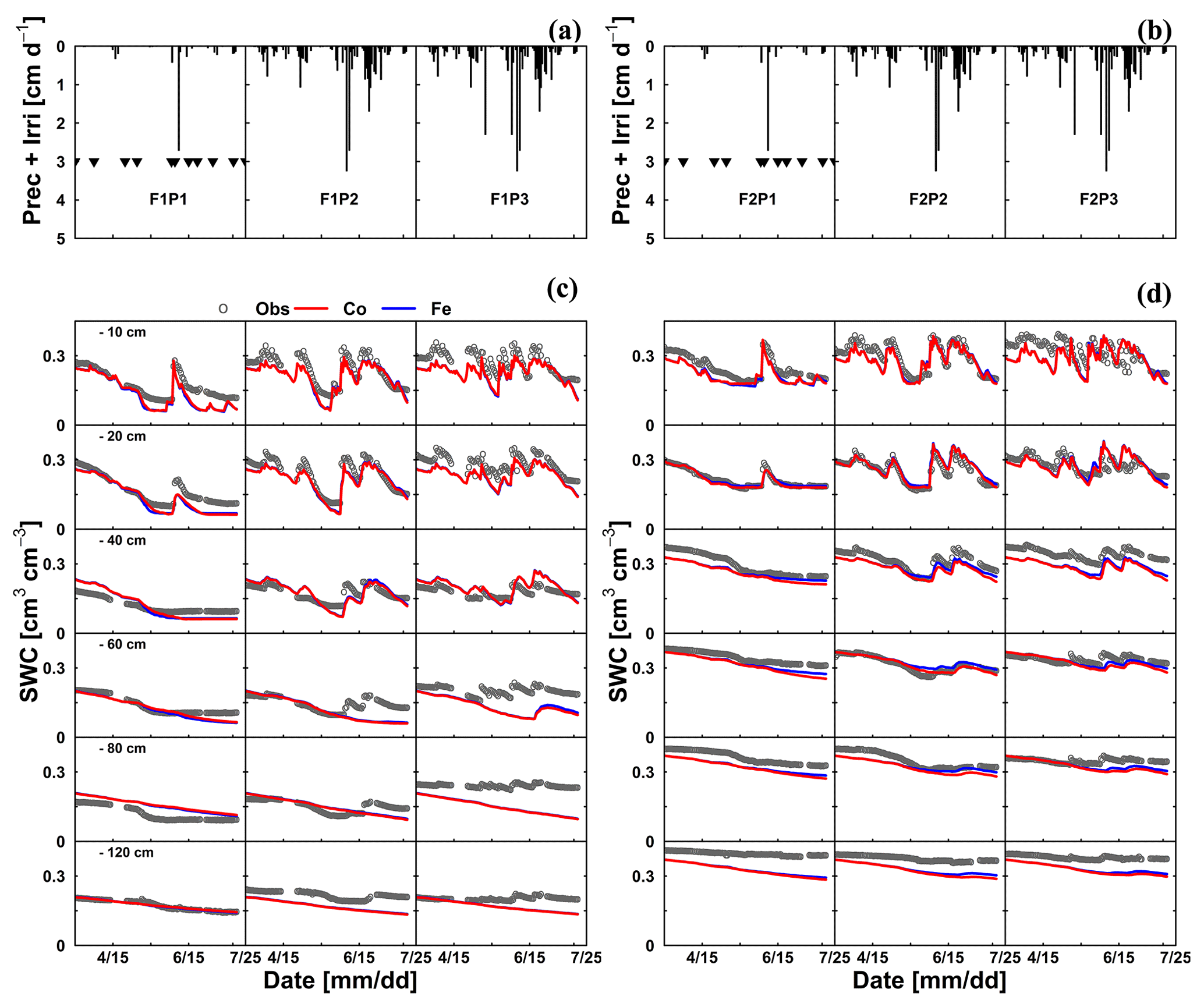
Figure 8 Illustrations of (a, b) time series of precipitation (Prec) and irrigation (Irri) and comparison between observed (black) and simulated soil water content (SWC) by the Couvreur (Co; solid red) and Feddes RWU model (Fe; solid blue) at six soil depths in the sheltered (P1), rainfed (P2), and irrigated (P3) plots of (c) the stony soil (F1) and (d) the silty soil (F2) from 15 March to 23 July 2016. Triangle symbols in the sheltered plots (F1P3 and F2P3) indicate the sheltered events.

For a few selected days, the diurnal course of T_act (or RWU), gross assimilation rate (P_g), stomatal conductance (g_s), and leaf pressure head was measured. The measured and simulated data are shown in Fig. 9. Both Co and Fe models could mimic the daytime fluctuation of RWU and P_g in the sheltered plot of the stony soil, which is consistent with the adequate simulation of root growth (Fig. 4, F1P1) and SWC dynamics (Fig. 8c, F1P1). When the simulated ψ_leaf reached ${\mathit{\psi }}_{\mathrm{threshold}}=-\mathrm{200}$ m, the simulated RWU and P_g by the Co model showed a plateau (26 May in Fig. 9c, e, and i). The Co model simulated the diurnal courses of stomatal conductance better as compared to the Fe model, especially on a day with water stress (26 May; Fig. 9g and h). Using the leaf water pressure head threshold as an indication of water stress effects on stomata, Tuzet et al. (2003) and Olioso et al. (1996) also reported a considerable drop of P_g and transpiration. The sharp drop of simulated RWU and P_g, which is in contrast with measurement on the same day in the sheltered plot in silty soil, illustrated that both models overestimated the water stress. This is related to the underestimation of both root growth (Fig. 4, F2P1) and SWC (Fig. 8d, F2P1) in the deeper soil layers by two models.

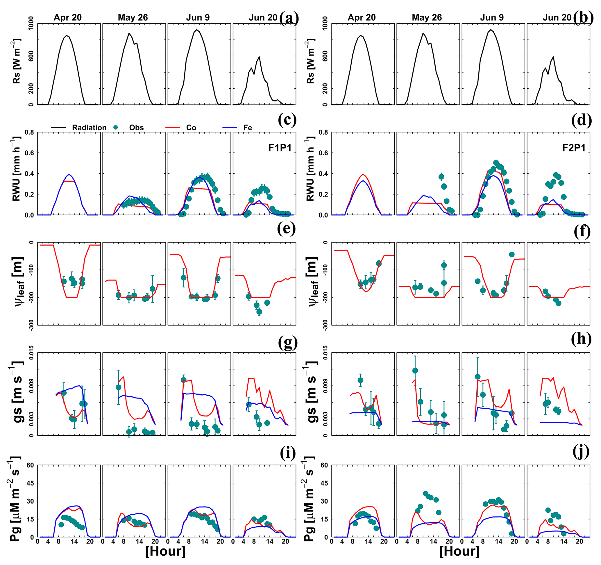
Figure 9 Diurnal courses of 4 selected measurement days: 20 April, 26 May, 9 June, and 20 June 2016. (a, b) Global radiation (Rs), (c, d) actual transpiration (RWU), (e, f) leaf water pressure head (ψ_leaf), (g, h) stomatal conductance to water vapor (g_s), and (i, j) gross assimilation rate (P_g) in the sheltered plot (P1) of the stony soil (F1) and the silty soil (F2). The cyan dots denote the observed values, and the solid red lines and solid blue lines denote the simulated values from the Couvreur model (Co) and Feddes model (Fe), respectively. Sap flow sensors were installed on 26 May 2016 at 09:00 and 17:00 LT for F1P1 and F2P1, respectively. Simulated stomatal conductance is from sunlit leaves. The Feddes RWU model did not simulate the leaf water pressure head.

3.1.3 Whole plant hydraulic conductance from the Couvreur RWU model

The Couvreur RWU model considers the root hydraulic conductance, which relies on absolute root length. The root hydraulic conductance is used to upscale to whole plant hydraulic conductance. The simulated K_plants reproduced the measured ones in the different treatments quite well (Fig. 10). Our measured K_plant ranged from $\mathrm{1.5}\times {\mathrm{10}}^{-\mathrm{5}}$ to $\mathrm{10.2}\times {\mathrm{10}}^{-\mathrm{5}}$ d⁻¹ (Fig. 10). These values are on the same order of magnitude as values reported by Feddes and Raats (2004) for ryegrass ranging from $\mathrm{6}\times {\mathrm{10}}^{-\mathrm{5}}$ to $\mathrm{20}\times {\mathrm{10}}^{-\mathrm{5}}$ d⁻¹. The simulated K_plant from our coupled root and shoot Co model followed the root growth and reached a maximum at around anthesis. K_plant reduces toward the end of the growing season due to root death. For the sheltered plot of the silty field, we would expect, based on the root density measurements (Fig. 4), the highest K_plant of all treatments. However, this was not observed in the field. Based on the measured total root lengths, we would also expect that K_plant of the sheltered plot in the stony soil should be similar to K_plant in the other plots of the stony soil. But, K_plant was clearly lower in the sheltered plot of the stony soil than in the other treatments in the stony soil. In the model simulations, the lower K_plant in the sheltered plots compared to the other plots in the same soil was due to a lower simulated total root length. Since the differences in observed total root lengths were smaller (stony soil) or opposite (silty soil) to the differences in simulated total root lengths, the smaller observed K_plant in the sheltered plots must have causes that are not considered in the model. A potential candidate is the resistance to water flow from the soil to the root in the soil, which increases considerably when the soil dries out, as was the case in the sheltered field plots.

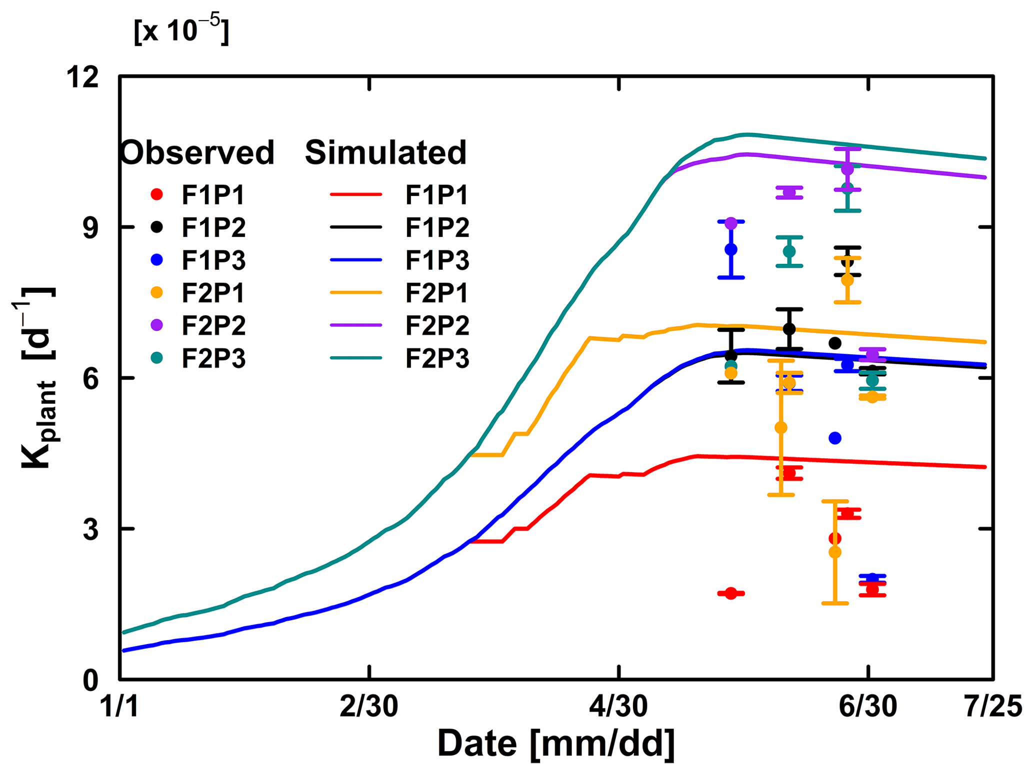
Figure 10 Comparison between observed (dot) and simulated plant hydraulic conductance (solid line) by the Couvreur (Co) model in the sheltered (P1), rainfed (P2), and irrigated (P3) plots of the stony soil (F1) and the silty soil (F2). The vertical bars represent the standard deviation of six hourly plant hydraulic conductance values at around midday (11:00 to 16:00 LT) on the measurement day. Note that crop germination was on 26 October 2015; data are shown here from 1 January to harvest on 23 July 2016. The blue line was overlapped by the black line.

The observed field data have been shown and compared with the simulated results from the two models in the abovementioned sections, Sect. 3.1.1–3.1.3. The data were collected for both crop growth (root, LAI, and biomass) and gas fluxes at different scales (soil water flux and gas exchange from leaf to canopy) in two contrast soil types and under different water treatments. To the best of our knowledge, this is a unique experimental setup and dataset for understanding soil–plant processes as well as parameterizing and evaluating soil–plant–atmospheric models. However, due to complex and costly construction of the underground minirhizotron facilities, there were no replicates for plots in our study. LAI and aboveground biomass showed the largest variability, not only between water treatments but even in the same plot because of microclimate and soil heterogeneities. The variability of tiller development also considerably influences the stem-to-stem variability of sap flow. In addition, the small size of plot did not allow for having replicates for manual canopy chamber measurement because it might strongly have disturbed and altered crop growth, leaf gas exchange, and sap flow measurements of the surrounding areas. Nevertheless, despite these shortcomings, the data illustrated the difference and variability among water regimes in two soil types and over measured dates that are still valid for modeling comparison and validation in this study.

3.2 Effects of changing root hydraulic conductance and leaf water pressure head thresholds

We conducted three sets of simulations. In the first set of simulations $K_{r_{\mathrm{s}},\mathrm{normalized}}$ was changed. Figure 11 illustrates the sensitivity of the Co model to $K_{r_{\mathrm{s}},\mathrm{normalized}}$ in terms of aboveground biomass at harvest and cumulative RWU (from 15 March to harvest) for the different water treatments and soil types. For the rainfed and irrigated plots, an increase in $K_{r_{\mathrm{s}},\mathrm{normalized}}$ does not lead to a substantial increase in RWU and aboveground biomass. This is a trivial consequence of the fact that water is not (irrigated plots) or only slightly (rainfed plots) limited in these cases. For the stony soil, a decrease of $K_{r_{\mathrm{s}},\mathrm{normalized}}$ by a certain factor leads to a stronger decrease in RWU and biomass than in the silty soil. This indicates that in the stony soil, less water is “accessible” so that a decrease in root water uptake capacity by the crop has a stronger impact on RWU and biomass production than in the silty soil. For the sheltered plots, RWU and biomass production increase with $K_{r_{\mathrm{s}},\mathrm{normalized}}$, suggesting that increasing the water uptake capacity by the plants would increase the uptake and growth. But, increasing $K_{r_{\mathrm{s}},\mathrm{normalized}}$ by the same factor had a smaller relative effect on the RWU and biomass production than decreasing $K_{r_{\mathrm{s}},\mathrm{normalized}}$.

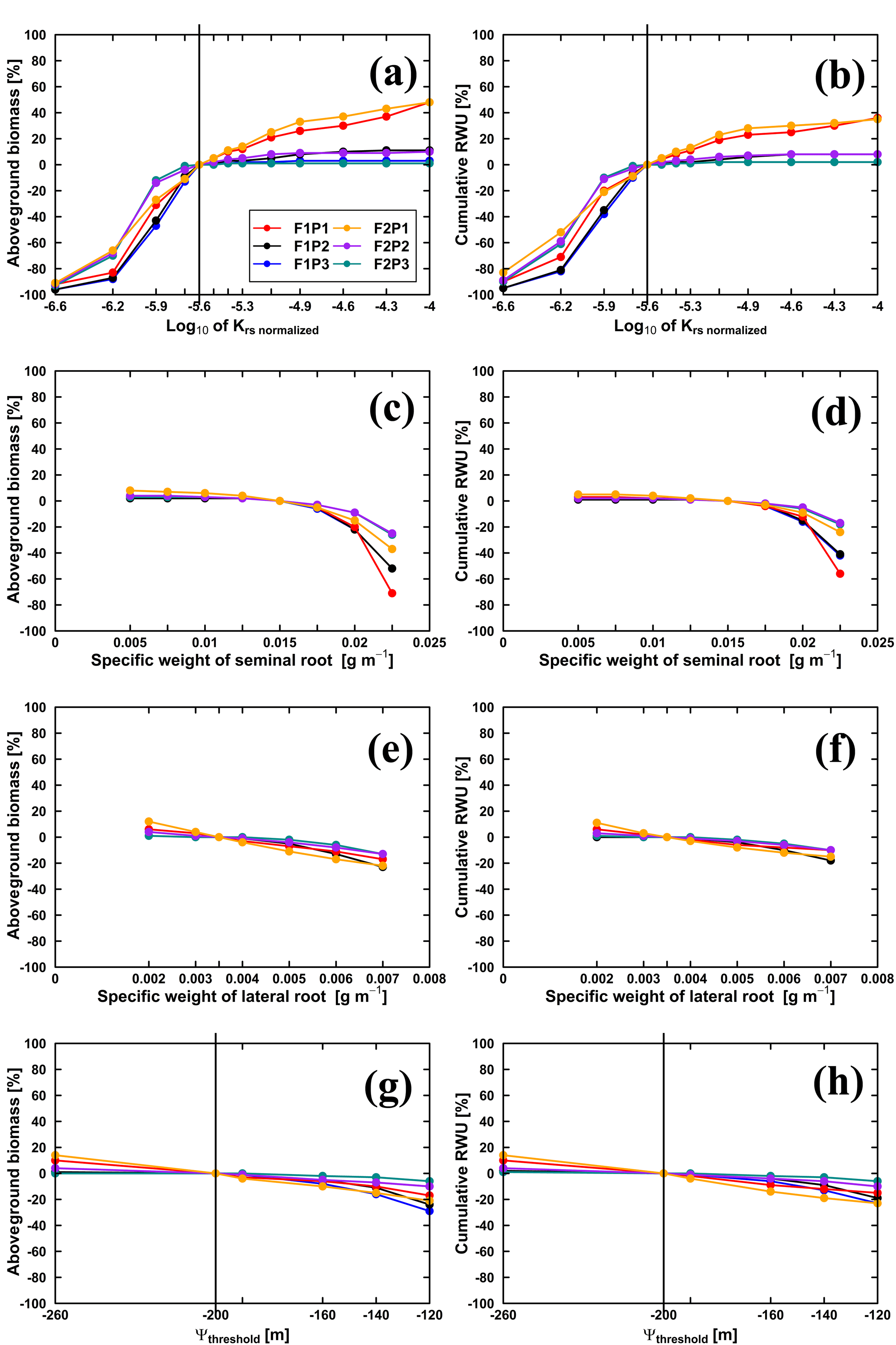
Figure 11 Relative changes of simulated (Co model) aboveground biomass at harvest (a, c, e, g) and cumulative RWU (b, d, f, h) (from 15 March to harvest on 23 July 2016) with the changing $K_{r_{\mathrm{s}},\mathrm{normalized}}$, specific weights of seminal and lateral roots and leaf pressure head threshold (Ψ_threshold) in the sheltered (P1), rainfed (P2), and irrigated (P3) plots of the stony soil (F1) and the silty soil (F2). Vertical lines in (a, b) indicate the original value $K_{r_{\mathrm{s}},\mathrm{normalized}}=\mathrm{0.2554}\times {\mathrm{10}}^{-\mathrm{5}}$ (cm d⁻¹), while in (g, h) the vertical lines indicate the ${\mathrm{\Psi }}_{\mathrm{threshold}}=-\mathrm{200}$ m.

Decreasing the specific weight of lateral and seminal roots increases the specific root length and thus the total root length of the root system as well as the total root system hydraulic conductance and thus the whole plant hydraulic conductance. However, for the considered range of specific weights, there was only a minor increase of aboveground dry biomass and RWU (Fig. 11c–f). Reducing the specific root length by increasing the specific weights of lateral and seminal roots caused a stronger reduction in biomass and RWU, especially for the seminal roots in the stony soil. High values of Ψ_threshold led to more water stress and a sharp decrease in stomatal conductance and photosynthesis when Ψ_leaf was limited to its thresholds (Fig. 11g and h). Our results suggested that Ψ_threshold at −120 or −140 m could overestimate the water stress, while Ψ_threshold at −260 m could underestimate the stress.

The impact of the change of the root segment conductance, specific weight of roots, and the leaf pressure head threshold at which stomata close on RWU and aboveground biomass is amplified by the positive feedback between the aboveground biomass, the root biomass, the total root length, the root system hydraulic conductance, and finally K_plant. Considering these interactions and feedbacks is important to evaluate the impact of changing a certain property of the crop on its performance in different soils and under different conditions.

The impact of changing root system properties or stomatal sensitivity to water pressure head on root water uptake, stress, and crop growth cannot be assessed by a model that is not sensitive to these crop properties. Different to the Co model, the Fe model is not sensitive to the total root length, the normalized root conductance, the specific root weight, and the leaf water hydraulic head at which stomata close. Therefore, the impact of introducing crop varieties with new properties cannot be assessed by this type of model. Only with the Co model can the impact of the crop properties on growth and drought resilience be studied.

4 Conclusion

We evaluated two different root water uptake modules of a coupled soil water balance and crop growth model. One root water uptake model was the commonly used Feddes model, whereas the other, the Couvreur RWU model, represents a “mechanistic” RWU that explicitly simulates the continuum in water potential from the soil to roots and to leaves based on the whole plant hydraulic conductance. Overall, the measured biomass growth, LAI development, soil water contents, leaf water pressure heads, and transpiration rates were well reproduced by both models. But, the Fe model incorrectly predicted more water stress and less growth in the silty soil than in the stony soil, whereas the opposite was observed. The Fe model does not account for the higher plant conductance in the silty soil where more roots were simulated than in the stony soil. In addition, the Fe model does not consider root water uptake compensation which reduces water stress. In other words, the Feddes approach did not possess the flexibility as compared to the Couvreur model in simulating RWU for different soil and water conditions.

Based on the absolute root length, the Co model was able to simulate K_plant in different soils and treatments. The simulated K_plant followed the root growth and reached a maximum at around anthesis. However, the observed K_plant was lower in the sheltered plots, although the observed total root lengths in these plots were almost similar (stony soil) or larger (silty soil) as compared to the irrigated and rainfed plots. Moreover, the higher simulated K_plant in comparison to the observed values in the sheltered plots suggested that the newly coupled model needs to consider the declined hydraulic conductance of the root–soil interface due to decreased soil water pressure head. The formation of air gaps at the soil–root interface due to the root shrinkage of roots and root–soil contact loosening (Carminati et al., 2009) could induce a strong increase of hydraulic resistance to radial water flow between soil and roots.

A mechanistic model that is based on plant hydraulics and links root system properties to RWU, water stress, and crop development can evaluate the impact of certain crop properties (change of root segment conductance, specific weights of root, or leaf pressure head thresholds) on crop performance in different environments and soils. The Co model could capture the positive feedbacks between the aboveground biomass, the root length, the total root system hydraulic conductance, and finally K_plant.

In this study, a higher total root length was simulated in the silty soil than in the stony soil because a higher specific root length was found for root growth in the silty soil. This can be considered as an extra relationship that requires attention in crop modeling. Crop growth models will need to consider soil specific calibration to account for differences in specific root length with soil. Alternatively, a more mechanistic description of root growth that predicts root specific length would reduce the amount of calibration in crop growth models. Another aspect in demand of improvement is the prediction of the root distribution with depth. In our simulations, the highest root densities were simulated in the topsoil, whereas the observations showed higher densities in the deeper soil layers. Examples of detailed 3-D root growth models that could improve the simulation of root distribution are given by Dunbabin et al. (2013). The coupling of a shoot model with a 3-D root growth model that represents root system architecture simulated more accurate root distributions (in both topsoil and subsoil layers) under drought conditions (Mboh et al., 2019). Nevertheless, simulating the third dimension of root growth would largely extend the parameter requirements, which makes them more difficult for testing under the field.

Finally, the model did not consider changes in carbon allocation to the root system that are triggered by stress. Therefore, the model simulated fewer roots in the water-stressed sheltered plot of the silty soil, whereas more roots were observed in this plot compared with the other plots in this soil. A more mechanistic description of root–shoot partitioning of both carbon and nitrogen (Yin and Schapendonk, 2004) or carbon allocation as a function of soil water conditions (i.e., soil water potential in Kage et al., 2004, and Li et al., 1994) would be needed to refine the prediction of responses of root development to water stress.

Future research should focus on testing the newly coupled model (HILLFLOW–Couvreur's RWU–SLIMROOT–LINTULCC2) for other wheat genotypes and crop types (isohydric like maize) and for a wider range of soil and climate conditions. Further improvements should particularly target leaf area simulation. Improving the modeling of leaf growth should result in better simulations of LAI and more accurate estimates of energy fluxes at the canopy level.

Appendix A: Leaf photosynthesis and stomatal conductance calculation

$$\begin{array}{}\text{(A1)}& {\displaystyle }& {\displaystyle }{\mathrm{AMAX}}_{l,t}={\displaystyle \frac{{\mathrm{VCMAX}}_{l,t}\left(C_{{\mathrm{i}}_{l,t}}-{\mathrm{\Gamma }}^{*}\right)}{C_{{\mathrm{i}}_{l,t}}+\mathrm{KMC}\left(\mathrm{1}+\frac{{\mathrm{O}}_{\mathrm{2}}}{\mathrm{KMO}}\right)}}{f}_{\mathrm{wat}}\text{(A2)}& {\displaystyle }& {\displaystyle }{\mathrm{EFF}}_{l,t}={\displaystyle \frac{J}{\mathrm{2.1}}}{\displaystyle \frac{C_{{\mathrm{i}}_{l,t}}-{\mathrm{\Gamma }}^{*}}{\mathrm{4.5}\left(C_{{\mathrm{i}}_{l,t}}+\mathrm{2}{\mathrm{\Gamma }}^{*}\right)}}\text{(A3)}& {\displaystyle }& {\displaystyle }{\mathrm{FGR}}_{l,t}={\mathrm{AMAX}}_{l,t}\left(\mathrm{1}-e^{-I_{l,t}\frac{{\mathrm{EFF}}_{l,t}}{{\mathrm{AMAX}}_{l,t}}}\right)\text{(A4)}& {\displaystyle }& {\displaystyle }{C}_{{\mathrm{i}}_{l,t}}=C_{\mathrm{a}}-\left({\mathrm{FGR}}_{l,t}{\displaystyle \frac{\mathrm{1}}{g_{{\mathrm{s}}_{l,t}}}}\right)\text{(A5)}& {\displaystyle }& {\displaystyle }{g}_{{\mathrm{s}}_{l,t}}=a_{\mathrm{1}}+{\displaystyle \frac{b_{\mathrm{1}}{\mathrm{FGR}}_{l,t}}{\left(C_{{\mathrm{i}}_{l,t}}-{\mathrm{\Gamma }}^{*}\right)\left(\mathrm{1}+\frac{{\mathrm{DS}}_{l,t}}{D_{\mathrm{0}}}\right)}}{f}_{\mathrm{wat}}\end{array}$$

AMAX is light saturated leaf photosynthesis (µM CO₂ m⁻² s⁻¹); VCMAX is the maximum carboxylation rate of the rubisco enzyme (µM m⁻² s⁻¹); C_i is the intercellular CO₂ concentration (µM mol⁻¹); C_a is the atmospheric CO₂ concentration (µM mol⁻¹); KMC is the Michaelis–Menten constant for CO₂ (µM mol⁻¹); KMO is the Michaelis–Menten constant for O₂ (µM mol⁻¹); O₂ is the atmospheric oxygen concentration (µM mol⁻¹); Γ^* is the CO₂ compensation point (µM mol⁻¹); EFF is the quantum yield (µM CO₂ MJ⁻¹); J is the conversion energy from radiation to mole photon (mole photons per MJ); FGR is the leaf photosynthesis rate (µM CO₂ m⁻² s⁻¹); I is the total absorbed flux of radiation (MJ m⁻² s⁻¹); g_s is the bulk stomatal conductance (mol m⁻² s⁻¹); a₁ is the residual stomatal conductance (mol m⁻² s⁻¹) when FGR = 0; b₁ is the fitting parameter (–); DS is the vapor pressure deficit at the leaf surface (Pa); D₀ is the empirical coefficient reflecting the sensitivity of the stomata to VPD (Pa); l is a sub-index that indicates the canopy layer (sunlit and shaded leaf) (–); t is a sub-index that indicates the time of the day (–); f_wat is the water stress factor for stomatal conductance and maximum carboxylation rate (–).

Appendix B: Scaling up of leaf stomatal conductance to canopy resistance in an hourly simulation

To scale up from leaf stomatal conductance to the canopy level and for computation efficiency, we approximate the integrals

$$\underset{\mathrm{0}}{\overset{\mathrm{LAI}}{\int }}f\left(l\right)dl.$$

By Gaussian quadrature, LAI$\sum _{j=\mathrm{1}}^{\mathrm{5}}{w}_j\cdot f(\mathrm{LAI}\cdot x_j)$, where x_j are the nodes and w_j the weights of the five-point Gaussian quadrature (Goudriaan and van Laar, 1994). LAI is the leaf area index, and f is a function dependent on leaf area, for instance gsH₂O. The abovementioned bulk stomatal conductance to CO₂ ($g_{{\mathrm{s}}_{l,t}}$ in mol m⁻² s⁻¹) of sunlit and shaded leaf to stomatal conductance was converted to stomatal conductance to H₂O (m s⁻¹) based on the molar density of air.

$$\begin{array}{}\text{(B1)}& {\displaystyle }& {\displaystyle }\mathrm{gs}{{\mathrm{H}}_{\mathrm{2}}\mathrm{O}}_{\mathrm{sun}}=\mathrm{1.56}\cdot {\mathrm{gs}}_{\mathrm{sun}}/\mathrm{41.66}\text{(B2)}& {\displaystyle }& {\displaystyle }\mathrm{gs}{{\mathrm{H}}_{\mathrm{2}}\mathrm{O}}_{\mathrm{shade}}=\mathrm{1.56}\cdot {\mathrm{gs}}_{\mathrm{shade}}/\mathrm{41.66}\end{array}$$

Leaf stomatal conductance to H₂O (m s⁻¹) was calculated based on the fraction of sunlit leaf area FSLLA:

$$\begin{array}{}\text{(B3)}& \mathrm{gs}{{\mathrm{H}}_{\mathrm{2}}\mathrm{O}}_{\mathrm{leaf}}=\mathrm{gs}{{\mathrm{H}}_{\mathrm{2}}\mathrm{O}}_{\mathrm{sun}}\cdot \mathrm{FSLLA}+\mathrm{gs}{{\mathrm{H}}_{\mathrm{2}}\mathrm{O}}_{\mathrm{shade}}(\mathrm{1}-\mathrm{FSLLA}).\end{array}$$

The hourly canopy conductance HourlyGSCropH2O (m s⁻¹) was calculated in Eq. (B4):

$$\begin{array}{}\text{(B4)}& \mathrm{HourlyGSCropH}\mathrm{2}\mathrm{O}=\mathrm{LAI}\cdot \sum _{j=\mathrm{1}}^{\mathrm{5}}{w}_j\mathrm{gs}{{\mathrm{H}}_{\mathrm{2}}\mathrm{O}}_{\mathrm{leaf}}.\end{array}$$

Hourly canopy resistance (s m⁻¹) was the reciprocal of hourly canopy conductance

$$\begin{array}{}\text{(B5)}& {\mathrm{Hr}}_{\mathrm{s}}=\mathrm{1}/\mathrm{HourlyGSCropH}\mathrm{2}\mathrm{O}.\end{array}$$

Hourly aerodynamic resistance (r_a) was calculated as Eq. (4) in Chapter 2 in the FAO Irrigation and Drainage Paper No. 56 (Allen et al., 1998). Assuming the leaf cuticle resistance and soil surface resistance were minor and neglected, the calculated canopy resistance (Hr_s) with f_wat=1 was directly used to calculate hourly crop evapotranspiration (ETP) using the Penman–Monteith equation (Eq. B6; see Eq. 3, Chapter 2, in the FAO Irrigation and Drainage Paper No. 56, Allen et al., 1998).

$$\begin{array}{}\text{(B6)}& \mathrm{ETP}={\displaystyle \frac{\mathrm{\Delta }\left(R_{\mathrm{n}}-G\right)+{\mathit{\rho }}_{\mathrm{a}}{c}_{\mathrm{p}}\frac{\left(e_{\mathrm{s}}-e_{\mathrm{a}}\right)}{r_{\mathrm{a}}}}{\mathit{\lambda }\left(\mathrm{\Delta }+\mathit{\gamma }\left(\mathrm{1}+\frac{{\mathrm{Hr}}_{\mathrm{s}}}{r_{\mathrm{a}}}\right)\right)}}\end{array}$$

R_n is net radiation (MJ m⁻² h⁻¹); G is soil heat flux (MJ m⁻² h⁻¹); e_s is saturation vapor pressure at the air temperature (kPa); e_a is actual vapor pressure at the air temperature (kPa); ρ_a is mean air density at constant pressure (kg m⁻³); c_p is the specific heat at constant pressure of the air ($\mathrm{1.013}\times {\mathrm{10}}^{-\mathrm{3}}$ MJ kg^−1 ∘C⁻¹); Δ is the slope of the saturation vapor pressure–temperature relationship (kPa ^∘C⁻¹); γ is the psychrometric constant of instrument (kPa ^∘C⁻¹); Hr_s is canopy resistance (s m⁻¹); r_a is the aerodynamic resistance (s m⁻¹); λ is the latent heat of vaporization (2.45 MJ kg⁻¹).

Appendix C: Crop parameters used in the modeling work

Table C1 List of crop parameters used in the modeling work.

Appendix D: Soil physical parameters in the topsoil (0–30 cm) and subsoil (30–150 cm)

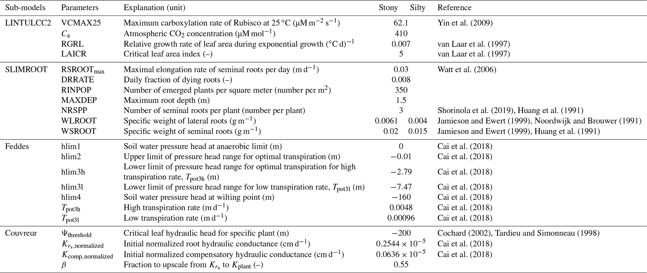
Table D1 Soil physical parameters in the topsoil (0–30 cm) and subsoil (30–150 cm).

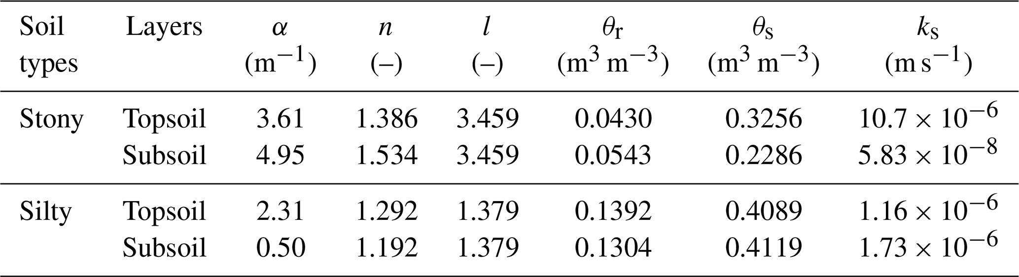
The θ_r and θ_s are residual and saturation soil water content, respectively; α, n, l are empirical coefficients affecting the shape of the van Genuchten hydraulic functions; k_s is the saturated hydraulic conductivity of the soil.

Appendix E: Feddes root water uptake model

The root water uptake in the HILLFLOW 1D model which is limited by soil water content in the root zone is calculated by reduction of potential transpiration (T_pot). The semi-empirical reduction function α(Ψ_m,i) is derived from the soil pressure head (Feddes et al., 1978). The α(ψ_m,i) also depends on T_pot because ψ₃ (soil pressure head where conditions for transpiration are optimal) is calculated via piecewise linear function of T_pot (Wesseling and Brandyk, 1985). The root water uptake was calculated based on the relative root length density which is output from the SLIMROOT root growth model.

$$\begin{array}{}\text{(E1)}& \begin{array}{rl}& \mathit{\alpha }\left({\mathit{\psi }}_{m,i}\right)=\\ & \left\{\begin{array}{ll}\mathrm{0}& {\mathit{\psi }}_{m,i}\ge {\mathit{\psi }}_{\mathrm{1}},{\mathit{\psi }}_{m,i}\le {\mathit{\psi }}_{\mathrm{4}}\\ \left({\mathit{\psi }}_{m,i}-{\mathit{\psi }}_{\mathrm{1}}\right)/\left({\mathit{\psi }}_{\mathrm{2}}-{\mathit{\psi }}_{\mathrm{1}}\right)& {\mathit{\psi }}_{\mathrm{2}}\le {\mathit{\psi }}_{m,i}\le {\mathit{\psi }}_{\mathrm{1}}\\ \mathrm{1}& {\mathit{\psi }}_{\mathrm{3}}\le {\mathit{\psi }}_{m,i}\le {\mathit{\psi }}_{\mathrm{2}}\\ \left({\mathit{\psi }}_{m,i}-{\mathit{\psi }}_{\mathrm{4}}\right)/\left({\mathit{\psi }}_{\mathrm{3}}-{\mathit{\psi }}_{\mathrm{4}}\right)& {\mathit{\psi }}_{\mathrm{4}}\le {\mathit{\psi }}_{m,i}\le {\mathit{\psi }}_{\mathrm{3}}\end{array}\right.\end{array}\end{array}$$

$$\begin{array}{}\text{(E2)}& \begin{array}{rl}& {\mathit{\psi }}_{\mathrm{3}}=\\ & \left\{\begin{array}{ll}{\mathit{\psi }}_{\mathrm{3}\mathrm{h}}& T_{\mathrm{pot}}>T_{\mathrm{3}\mathrm{h}}\\ {\mathit{\psi }}_{\mathrm{3}\mathrm{h}}+\frac{\left({\mathit{\psi }}_{\mathrm{3}\mathrm{l}}-{\mathit{\psi }}_{\mathrm{3}\mathrm{h}}\right)\left(T_{\mathrm{3}\mathrm{h}}-T_{\mathrm{pot}}\right)}{\left(T_{\mathrm{3}\mathrm{h}}-T_{\mathrm{3}\mathrm{l}}\right)}& T_{\mathrm{3}\mathrm{l}}<T_{\mathrm{pot}}<T_{\mathrm{3}\mathrm{h}}\\ {\mathit{\psi }}_{\mathrm{3}\mathrm{l}}& T_{\mathrm{pot}}<T_{\mathrm{3}\mathrm{l}}\end{array}\right.\end{array}\end{array}$$

α(Ψ_m,i) is the transpiration reduction as a function of the soil pressure head (–); Ψ₁ is the soil water pressure head at the anaerobic limit (m); Ψ₄ is the soil pressure head at wilting point (m); Ψ₂ and Ψ₃ are upper and lower limits of the pressure head for optimal transpiration (m), respectively; T_pot is potential transpiration (m d⁻¹); Ψ_3h is the lower limit of the pressure head range for optimal transpiration for a high transpiration rate, T_pot3h (m); T_3h is a high potential transpiration rate (m d⁻¹); Ψ_3l is the lower limit of the pressure head range for a low transpiration rate, T_pot3l (m); T_3l is a low potential transpiration rate (m d⁻¹).

Appendix F: Comparison ratio of the observed total root length from minirhizotubes to the simulated observed total root length from F1P2

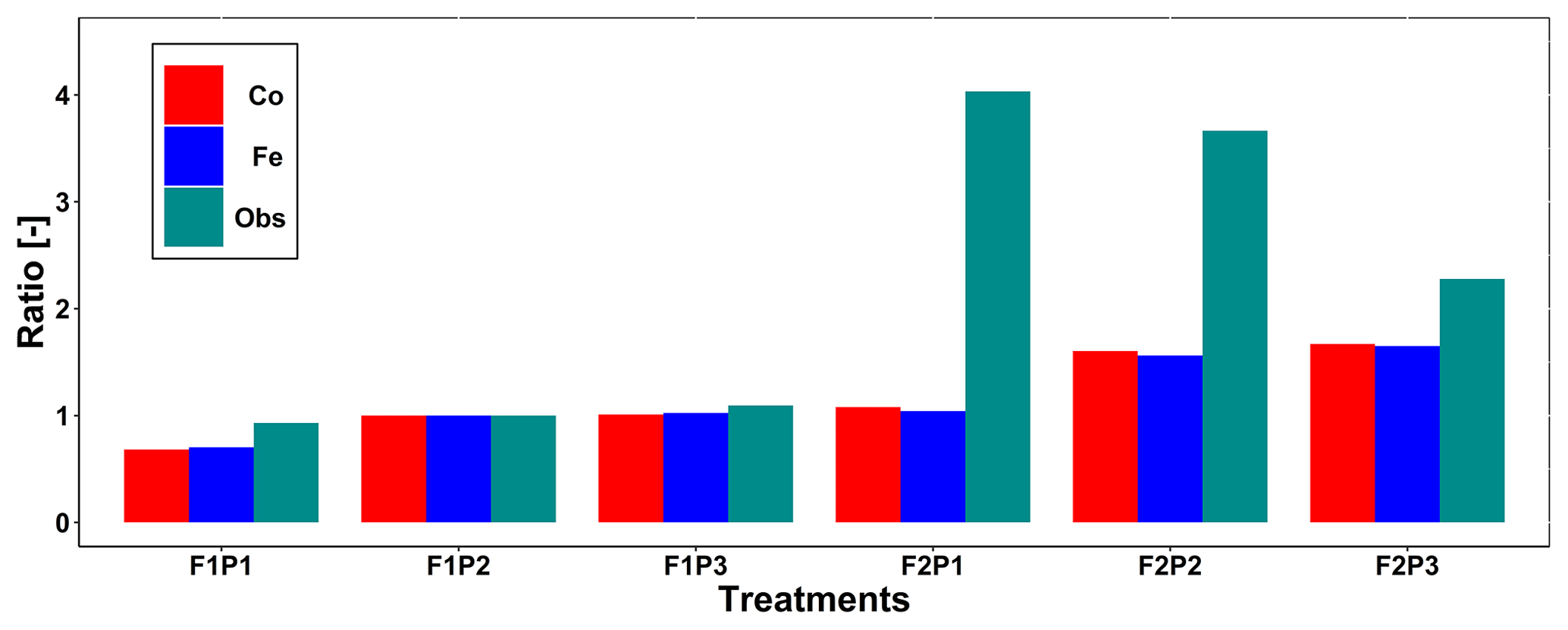
Figure F1 Comparison ratio of the observed total root length from minirhizotubes to observed total root length from F1P2 (green line with squares) and ratio of simulated total root length to the simulated total root length from F1P2 on 11 July 2016 (DOY 193) from the Couvreur (Co; solid red, dots) and Feddes (Fe; solid blue, triangles) model in the sheltered (P1), rainfed (P2), and irrigated (P3) plots of the stony soil (F1) and the silty soil (F2).

Appendix G: Summary of statistical RMSEs of soil water content simulated by two models

Table G1 Statistic RMSEs of soil water content simulated by the Couvreur (Co) and Feddes (Fe) models in the sheltered (P1), rainfed (P2), and irrigated (P3) plots of the stony soil (F1) and the silty soil (F2). RMSE is given in cm³ cm⁻³.