Coupled machine learning and the limits of acceptability approach applied in parameter identification for a distributed hydrological model

Monte Carlo (MC) methods have been widely used in uncertainty analysis and parameter identification for hydrological models. The main challenge with these approaches is, however, the prohibitive number of model runs required to acquire an adequate sample size, which may take from days to months – especially when the simulations are run in distributed mode. In the past, emulators have been used to minimize the computational burden of the MC simulation through direct estimation of the residual-based response surfaces. Here, we apply emulators of an MC simulation in parameter identification for a distributed conceptual hydrological model using two likelihood measures, i.e. the absolute bias of model predictions (Score) and another based on the time-relaxed limits of acceptability concept (pLoA). Three machine-learning models (MLMs) were built using model parameter sets and response surfaces with a limited number of model realizations (4000). The developed MLMs were applied to predict pLoA and Score for a large set of model parameters (95 000). The behavioural parameter sets were identified using a time-relaxed limits of acceptability approach, based on the predicted pLoA values, and applied to estimate the quantile streamflow predictions weighted by their respective Score. The three MLMs were able to adequately mimic the response surfaces directly estimated from MC simulations with an R² value of 0.7 to 0.92. Similarly, the models identified using the coupled machine-learning (ML) emulators and limits of acceptability approach have performed very well in reproducing the median streamflow prediction during the calibration and validation periods, with an average Nash–Sutcliffe efficiency value of 0.89 and 0.83, respectively.

1 Introduction

Conceptual hydrological models have a wide range of applications in solving various water quantity- and quality-related problems. A conceptual model typically comprises one or more calibration parameters, as part of the user's perception of the hydrological processes in the catchment, and the corresponding simplifications that are assumed to be acceptable for the intended modelling purpose (Beven, 1989; Refsgaard et al., 1997). One of the major challenges in using conceptual models, however, is the identification of model parameters for a particular catchment (e.g. Bárdossy and Singh, 2008). The failure to set parameter values in accordance with their theoretical bounds, the interaction between these parameters, and the absence of a unique best set of parameters are some of the causes of parameter uncertainty (Abebe and Price, 2003; Renard et al., 2010). In light of the different sources of uncertainty, previous studies have pointed out the need for a rigorous uncertainty analysis and the need to communicate model simulation results in terms of uncertainty bounds rather than with only crisp values (e.g. Uhlenbrook et al., 1999).

In the past, various uncertainty analysis techniques have been proposed to infer model parameter values from observations, including the generalized likelihood uncertainty estimation (GLUE) methodology (Beven and Binley, 1992), the dynamic identifiability analysis framework (DYNIA; Wagener et al., 2003), the Shuffled Complex Evolution Metropolis (SCEM) algorithm (Vrugt et al., 2003), and the Bayesian inference (Kuczera and Parent, 1998; Yang et al., 2007). The GLUE methodology was inspired by the generalized sensitivity analysis concept of Hornberger and Spear (1981), and it is the most widely used uncertainty analysis framework in hydrology (Stedinger et al., 2008; Xiong et al., 2009; Shen et al., 2012). The residual-based version of this framework allows the user to choose the likelihood and the threshold value to identify behavioural and nonbehavioural models. The limits of acceptability-based GLUE methodology (GLUE LoA; Beven, 2006) overcomes the limitations of the residual-based GLUE that arise from the subjectivity in choosing the likelihood and the threshold value by setting error bounds around the observed values. Models for which the prediction falls within the error bounds for all observations are considered behavioural. The original GLUE LoA, which was formulated as a rejectionist framework for testing environmental models as hypothesis, is too stringent to be used for calibration purposes, especially in continuous rainfall–runoff modelling. In the past, different approaches have been made to minimize the rejection of useful models when using GLUE LoA. These approaches include relaxing the limits (e.g. Blazkova and Beven, 2009; Liu et al., 2009), using different model realizations for different periods of a hydrological year (e.g. Choi and Beven, 2007), and using a time-relaxed approach with the degree of relaxation constrained by an additional efficiency criterion (Teweldebrhan et al., 2018). The time-relaxed GLUE LoA approach (hereafter referred to as GLUE pLoA) was based on the empirical relationship between model efficiency and uncertainty in response to the percentage of model predictions that fall within the observation error bounds (pLoA). In a case study involving this approach and an operational hydrological model, the ensemble of model realizations, with only 30 %–40 % of their predictions in a hydrological year falling within the observation error bounds, was able to predict streamflow during the evaluation period with an acceptable degree of accuracy for the intended use, based on the commonly used efficiency criteria.

Monte Carlo (MC) simulation is commonly employed to quantify the uncertainty propagated from model parameters to predictions in model calibration and uncertainty analysis frameworks, including the GLUE methodology. MC simulation involves the sampling of very large parameter sets from their respective parameter dimensions. This is especially true when the parameter distribution is not known a priori, and hence, a uniform distribution is assumed. Although the MC simulation is a widely accepted stochastic modelling technique, it suffers from a heavy computational burden (Yu et al., 2015). The computational time and resources required by the MC simulation could be prohibitively expensive in the case of computationally intensive models such as those with a distributed setup (e.g. Shrestha et al., 2014). In the past, different approaches were introduced to minimize the computational burden by reducing the number of model realizations in MC simulations. These included the use of more efficient parameter sampling techniques, such as the Latin hypercube sampling (e.g. McKay et al., 1979; Iman and Conover, 1980) and adaptive Markov chain MC sampling (e.g. Blasone et al., 2008; Vrugt et al., 2009), and through the use of emulators (e.g. Wang et al., 2015). An emulator or surrogate model is a computationally efficient model that is calibrated over a small data set obtained by the simulation of a computationally demanding model and is used in its place during computationally expensive tasks (Pianosi et al., 2016).

In hydrology, surrogate modelling has mainly been used in optimization and sensitivity analysis frameworks (Oakley and O'Hagan, 2004; Emmerich et al., 2006; Razavi et al., 2012). This approach involves a limited number of model realizations for building a surrogate model, using the parameter sets and model outputs as covariates and independent variables, respectively. Statistical models (e.g. Jones, 2001; Hussain et al., 2002; Regis and Shoemaker, 2004), Gaussian process models (Kennedy and O'Hagan, 2001; Yang et al., 2018), and machine-learning models (MLMs; e.g. Yu et al., 2015) have been used as surrogate models to emulate MC simulations. A machine-learning model estimates the dependency between the inputs and outputs of a system from the available data (Mitchell, 1997).

In this study three MLMs, i.e. random forest (RF), K nearest neighbours (KNN), and artificial neural network (NNET), are built using a limited number of model parameter sets and response surfaces to emulate the MC simulation through coupling with the limits of acceptability approach. In hydrology, machine-learning approaches have been increasingly used in different areas of application following the improvement in computational power. MLMs have been used in the direct prediction of different water quantity variables such as streamflow (Solomatine and Shrestha, 2009; Modaresi et al., 2018; Senent-Aparicio et al., 2018), evapotranspiration (Torres et al., 2011), and snow water equivalent (Marofi et al., 2011; Buckingham et al., 2015; Bair et al., 2018). Similarly, MLMs have been used to predict water-quality-related variables such as nitrate concentration (Ransom et al., 2017) and sediment transport (Bhattacharya et al., 2007). MLMs have also been used to forecast the residuals of a conceptual rainfall–runoff model (Abebe and Price, 2003) and as emulators to conduct the parameter uncertainty analysis of a conceptual hydrological model in order to overcome the high computational cost of the MC simulation (Shrestha et al., 2009). The main goal of this study is to emulate the time-consuming MC simulation for parameter identification through the coupling of machine-learning models with the time-relaxed limits of acceptability approach. The first objective is to assess the possibility of using pLoA as a likelihood measure for the identification of behavioural models by using the coupled MLMs and the limits of acceptability approach instead of the previously used residual-based likelihood measures. The second objective is to compare the relative performances of RF and KNN as emulators of the MC simulation in relation to the standard machine-learning-based emulator, i.e. NNET. To our best knowledge, RF and KNN have not been used before as emulators of the MC simulation in parameter identification for hydrological models. The third objective is to compare the performance of the MLMs trained using pLoA against those trained using the absolute bias-based criterion (Score) as target variables to conduct a sensitivity analysis in order to assess the relative influence of the model parameters on the simulation result.

This paper is structured as follows: Sect. 2 presents a brief introduction to parameter identification, using the time-relaxed GLUE LoA approach, and the MLMs used in this study. This section will also present the procedure followed in coupling the MLMs with the time-relaxed GLUE LoA to emulate the MC simulation. Section 3 introduces the hydrological model and the study area used in the case study. Section 4 presents the validation results of the ML models through a comparison of the predicted response surfaces against those directly generated from the MC simulation and a comparison of the simulated streamflow from behavioural models identified using the coupled MLMs and the time-relaxed GLUE LoA against the observed values. Implications of the results in relation to the data set and models used in this study, and relevant previous studies, are discussed in Sect. 5, and conclusions are drawn in Sect. 6.

2 Methodology

Coupling of the MLMs with the GLUE pLoA was realized in two main phases. In the first phase, the response surfaces were generated using a limited number of MC simulations, with a subsequent evaluation of each realization using pLoA and Score as likelihood measures. The MLMs were then built using the parameter sets and the response surfaces. In the second phase, the developed MLMs were applied to predict the response surfaces for the new parameter sets, and the GLUE pLoA was used to identify the behavioural parameter sets based on the predicted response surfaces. The R software and its package for classification and regression training (CARET) were used to build and apply the MLMs and to conduct further analyses.

2.1 Parameter identification using the time-relaxed limits of acceptability approach

The GLUE methodology (Beven and Binley, 1992) accepts the condition in which different behavioural model realizations give comparable model results, i.e. equifinality, as a working paradigm for parameter identification of hydrological models (Choi and Beven, 2007). The first step followed in implementing this methodology was identifying the uncertain model parameters and setting the range of their respective dimensions. The next step was randomly sampling the parameter sets from the prior distribution. Since the parameter distribution was not known a priori, a uniform MC sampling was employed. The hydrological model was run using the sampled parameter sets, and the streamflow predictions of all model realizations were retrieved for further analysis.

The GLUE limits of acceptability approach (GLUE LoA; Beven, 2006) was used to characterize behavioural and nonbehavioural simulations. This approach relies on an assessment of uncertainty in the observational data and involves setting an observation error bound (limit) with due consideration to the observation and other sources of uncertainties, such as from the input data. Since no streamflow uncertainty data were available in the study site, the mean observational uncertainty of 25 % was assumed, and the streamflow limits were defined using this value. In this study, the time-relaxed variant of the GLUE LoA (GLUE pLoA) was employed to characterize behavioural models. In GLUE pLoA, the requirement in the original formulation for the model realizations to satisfy the limits in 100 % of the observations is relaxed; the degree of relaxation is constrained as a function of an acceptable modelling uncertainty expressed by the containing ratio (CR) index. This index was also used to quantitatively evaluate the modelling and prediction uncertainties, following a similar procedure used in previous studies involving the GLUE methodology (e.g. Xiong et al., 2009). It is expressed as the number of observations, falling within their respective prediction bounds, to the total number of observations (Eq. 1). When using the GLUE methodology, the observations are not expected to lie within the prediction bounds at a percentage that equals the given certainty level. However, the modeller can adopt the certainty level specified to produce the prediction limits as a kind of standard for assessing the efficiency of the prediction limits in enveloping the observations (Beven, 2006).

$$\begin{array}{}\text{(1)}& \mathrm{CR}={\displaystyle \frac{\sum _{i=\mathrm{1}}^{n}I\left(Q_{\mathrm{obs},i}\right)}{n}},\end{array}$$

with

$$I\left(Q_{\mathrm{obs},i}\right)=\left\{\begin{array}{ll}\mathrm{1},& L_{\lim ,i}<Q_{\mathrm{obs},i}<U_{\lim ,i}\\ \mathrm{0},& \mathrm{otherwise}\end{array},\right.$$

where Q_obs,i represents observed streamflow at the i time step, and L_lim,i and U_lim,i, respectively, denote the lower and upper prediction bounds.

The percentage of observations where model predictions fall within the limits, i.e. pLoA, is estimated using Eq. (2).

$$\begin{array}{}\text{(2)}& \mathrm{pLoA}={\displaystyle \frac{\sum _{i=\mathrm{1}}^{n}S\left(Q_{\mathrm{sim},i}\right)}{n}}\times \mathrm{100},\end{array}$$

with

$$\begin{array}{c}{\displaystyle }S\left(Q_{\mathrm{sim},i}\right)=\left\{\begin{array}{ll}\mathrm{1},& {\mathrm{LQ}}_{\mathrm{e},i}<Q_{\mathrm{obs},i}<{\mathrm{UQ}}_{\mathrm{e},i}\\ \mathrm{0},& \mathrm{otherwise}\end{array}\right.\\ {\displaystyle }{\mathrm{LQ}}_{\mathrm{e},i}=Q_{\mathrm{obs},i}-\mathrm{0.25}\times Q_{\mathrm{obs},i}\\ {\displaystyle }{\mathrm{UQ}}_{\mathrm{e},i}=Q_{\mathrm{obs},i}+\mathrm{0.25}\times Q_{\mathrm{obs},i},\end{array}$$

where Q_sim,i represents simulated streamflow corresponding to the i observation, and LQ_e,i and UQ_e,i denote the lower and upper observation error bounds, respectively.

The procedure followed in GLUE pLoA to relax the original formulation is detailed in Teweldebrhan et al. (2018). For completeness, we include the following summary of the steps here:

• Step 1: define an acceptable modelling uncertainty (CR) at a chosen certainty level (e.g. 5 %–95 %) based on previous experience or literature values (e.g. Teweldebrhan et al., 2018). In this study, the CR value obtained for the calibration period using the residual-based GLUE methodology was adopted as an acceptable CR value.

• Step 2: relax the acceptable percentage of observations where model predictions fall within the limits. This is done by gradually lowering the requirement for bracketing the observations in 100 % of the time steps up to the acceptable pLoA.

• Step 3: test whether each model realization prediction falls within the limits – at least for the specified percentage of the total observations. If model realizations that satisfy the relaxed acceptability criteria are found, proceed to step 4; otherwise, lower the threshold pLoA further and repeat this step.

• Step 4: calculate the new CR, and check if it is close to the predefined acceptable CR value. If the calculated CR is less than the predefined CR, repeat steps 2 to 4. Whereas, if the two CR values are close (e.g. within 5 %), then accept all model realizations that satisfy this pLoA as behavioural, and store their indices for use in further analysis.

The identified behavioural model realizations were used to predict streamflow weighted by their respective Score values. When calculating Score, the prediction error, i.e. the deviation between the observed and simulated streamflow (Q) values (Q_obs−Q_sim), was first converted into a normalized criterion. This was accomplished using a triangular membership function, with its support representing the uncertainty in streamflow observations and the pointed core representing a perfect match between the observed and predicted values (Fig. 1). In Fig. 1 and the accompanying equations, μ_Q(e) denotes the membership grade of each prediction error (e) corresponding to the observed streamflow value i; m is the point in the support with a perfect match between the observed and predicted streamflow values. The variables L_e and U_e, respectively, refer to the lower and upper error bounds of the streamflow observations. The total Score (S_j) of each model realization, j, was calculated as the membership grade of the prediction error, summed over all observations (Eq. 3), and the normalized weight, in relation to the other model realizations (w_j), was calculated using Eq. (4) as follows:

$${\mathit{\mu }}_Q\left(e\right)=\left\{\begin{array}{ll}\mathrm{0},& e\le L_{\mathrm{e}}\\ {\displaystyle \frac{e-L_{\mathrm{e}}}{m-L_{\mathrm{e}}}},& L_{\mathrm{e}}<e\le m\\ {\displaystyle \frac{U_{\mathrm{e}}-e}{U_{\mathrm{e}}-m}},& m<e<U_{\mathrm{e}}\\ \mathrm{0},& e\ge U_{\mathrm{e}}.\end{array}\right.$$

$$\begin{array}{}\text{(3)}& {\displaystyle }{S}_j=\sum _{i=\mathrm{1}}^n{\mathit{\mu }}_Q\left(e\right)\text{(4)}& {\displaystyle }{w}_j={\displaystyle \frac{S_j}{\sum _{k=\mathrm{1}}^N{S}_k}},\end{array}$$

where the notations n and N, respectively, refer to the number of streamflow observations and behavioural models.

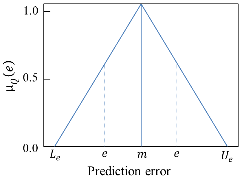
Figure 1 A triangular membership function for converting the streamflow prediction error into a normalized criterion.

2.2 Machine-learning modelling

Three nonlinear and nonparametric machine-learning methods, i.e. RF, KNN, and NNET from the CARET package of R (Kuhn, 2008), were considered in the emulation of the MC simulation. In all methods, the relevant parameters were optimized, and the root mean squared error (RMSE) metric was used to identify the optimal model. This section briefly summarizes these machine-learning methods, and the reader is referred to the reference above for detailed descriptions of these algorithms.

2.2.1 Random forest

Random forest (RF) is a version of the bagged tree (bootstrap-aggregated) algorithm (Breiman, 2001). As such, it is an ensemble method whereby a large number of individual trees are grown from random subsets of predictors, providing a weighted ensemble of trees (Bair et al., 2018). Bagging was reported to be a successful approach for combining unstable learners (e.g. Li et al., 2011). Since RF combines bagging with a randomization of the predictor variables used at each node, it yields an ensemble of low-correlation trees (Li et al., 2011; Appelhans et al., 2015). The free parameter in this method, i.e. the number of randomly selected predictors at each node, was determined through optimization. RF is also less sensitive to non-important variables since it implicitly performs variable selection (Okun and Priisalu, 2007).

2.2.2 K nearest neighbours

The K nearest neighbours (KNN) approach uses the K closest samples from the training data set to predict a new sample. The value of K, i.e. the number of closest samples used in the final model, was optimized. KNN is a nonparametric method in which the information extracted from the observed data sets is used to predict the variable of interest without defining a predetermined parametric relationship between the predictors and predicted variables (Modaresi et al., 2018). KNN is also a nonlinear method in which the prediction solely depends on the distance of the predictor variables to the closest training data set known to the model (Appelhans et al., 2015). In this study, the Euclidean distance was used as a similarity measure to compute the distance between the new and training data sets.

2.2.3 Artificial neural network

An artificial neural network (NNET) constitutes an interconnected and weighted network of several simple processing units called neurons that are analogous to the biological neurons of the human brain (Hsieh, 1993; Tabari et al., 2010). The neurons provide the link between the predictors and the predicted variable and, in the case of supervised learning, the weights of the neurons, i.e. the unidirectional connection strengths, are iteratively adjusted to minimize the error (Sajikumar and Thandavesware, 1999; Bair et al., 2018). NNET has the capability to detect and learn complex and nonlinear relationships between variables (Yu et al., 2015).

A multilayer perceptron is the most common type of neural network used in supervised learning (Zhao et al., 2005; Marofi et al., 2011), and it consists of an input layer in which input data are fed, one or more hidden layers of neurons in which data are processed, and an output layer that produces the output data for the given input (e.g. Senent-Aparicio et al., 2018). In this study one middle layer was considered, with the number of neurons in the input and output layers being equal to the number of predictors and predicted variable, respectively. The two free parameters of NNET, i.e. the number of neurons in the middle layer and the value of weight decay, were optimized. Based on a preliminary assessment of the performances of models with a linear and sigmoid activation function, a linear activation function was used in the final model.

2.3 Coupling of the machine-learning emulators with the limits of acceptability approach

The procedure followed in building and applying the MLMs as emulators of the MC simulation is similar to the approach used in previous studies (e.g. Yu et al., 2015), with the exception of the parameter identification. While the previous studies were conducted based on the residual-based GLUE, here we use the time-relaxed GLUE LoA approach with two likelihood measures. The coupling procedure involved the sampling of 5000 random samples from the dimensions of the uncertain model parameters. The hydrological model was run using these parameter sets with subsequent retrievals of the simulated streamflow values. Each model realization was evaluated in terms of its capability to generate simulated streamflow close to the observed values (Score) and its persistency in producing acceptable simulated values that fall within the observation error bounds (pLoA). Six MLMs (for the combinations of the two likelihoods, i.e. Score and pLoA, and for the three ML methods, i.e. RF, KNN, and NNET) were trained and tested using the randomly selected parameter sets and their corresponding likelihood values directly estimated from the MC simulation. Sample sizes of 80 % (S1) and 20 % (S2) of the 5000 samples were used, respectively, to train and test the MLMs (Table 1).

Table 1 Parameter samples used in the building and application of the MLM-based emulators.

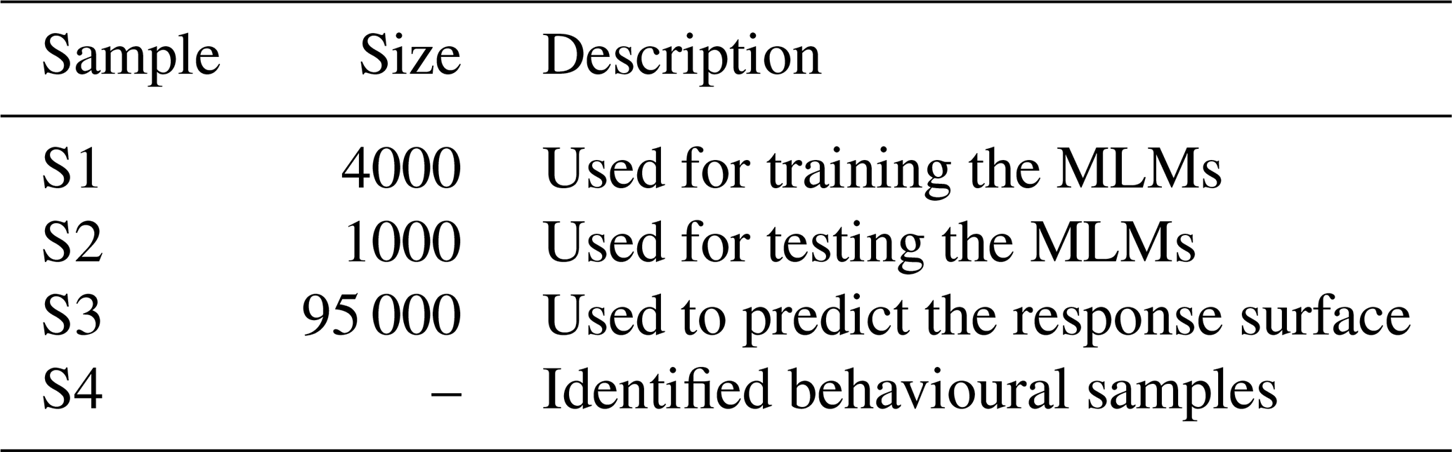
The trained MLMs were applied to emulate the MC simulation through the prediction of the likelihood measures corresponding to a much bigger size of randomly generated parameter sets, i.e. 95 000 (S3). For further validation of the MLMs, an MC simulation was also run using the hydrological model and the S3 parameter sets, with subsequent retrievals of the simulated streamflow and estimations of the two likelihood measures through comparison of the simulated against observed streamflow values. The performance of the surrogate models in the emulation of the MC simulation was evaluated through a comparison of their likelihood prediction against those estimated from the MC simulation. The identification of behavioural parameter sets (S4) from the S3 samples was realized using the time-relaxed GLUE LoA approach based on the MLM-predicted pLoA values of the samples. The Score-weighted streamflow predictions of these behavioural models were calculated at different quantile values. Performance of the three MLMs as emulators of the MC simulation was further assessed through cross-validation of the streamflow predictions of the behavioural models identified using each MLM coupled with GLUE pLoA (MLM–GLUE-pLoA) against observed values in the remaining years, other than the one used for building the MLM–GLUE-pLoA.

The procedure followed in building and evaluating MLM–GLUE-pLoA can be divided into two main phases as outlined below and depicted in the schematic overview in Fig. 2:

• a.

  MLM training and testing

  • i.

    Sample 5000 parameter sets randomly from their respective parameter dimensions.

  • ii.

    Run the hydrological model using the sampled parameter sets, and store the simulated streamflow corresponding to each parameter set.

  • iii.

    Calculate the performance of each model realization in terms of the percentage of time steps it is able to reproduce the observed streamflow within the observation error bounds, i.e. pLoA, and the total normalized absolute bias of the predicted streamflow (Score). A streamflow observation error bound of 25 % was assumed in this study.

  • iv.

    Use 80 % of the parameter sets, i.e. S1, of the samples generated in step (i) as covariates; use the performance of each parameter set (pLoA) calculated at the previous step as target variables to train the MLMs, i.e. RF, KNN, and NNET (MLMs_pLoA). Similarly, train the three MLMs using the same parameter sets (S1) as covariates but with Score as a target variable (MLMs_score).

  • v.

    Test the trained MLMs_pLoA using the remaining 20 % of the parameter sets generated in step (i), i.e. S2, and the corresponding target variable (pLoA) from step (iii). Similarly, test the trained MLMs_score using the same samples (S2) but with Score as a target variable.

• b.

  Response surface estimation and behavioural model identification

  • i.

    Repeat step (i) in MLM training and testing (a) but with a much bigger sample size of 95 000 (S3).

  • ii.

    Predict pLoA and Score using MLMs_pLoA and MLMs_score, respectively, and S3 as a covariate.

  • iii.

    Identify behavioural samples (S4) from S3 using the time-relaxed limits of acceptability approach (Sect. 2.1) based on the pLoA predicted by the MLM.

  • iv.

    Estimate the weighted median streamflow prediction of the behavioural models. The Score predicted by the MLMs_score was first normalized using Eq. (4) and then used to weigh the relative contribution of each model realization.

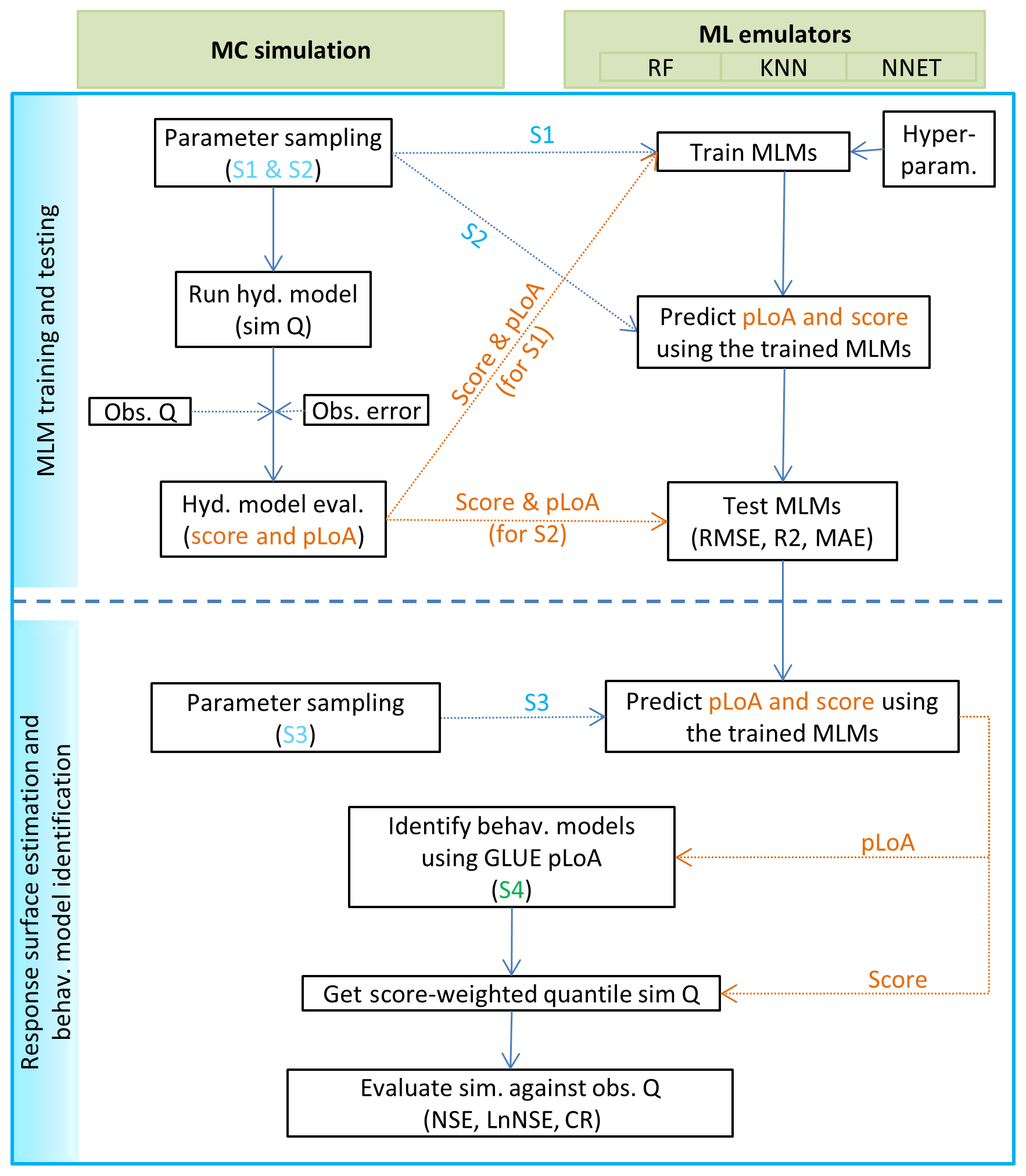
Figure 2 Schematic overview of the MLM training and testing, response surface prediction using the MLMs, and the identification of behavioural models using the coupled MLM and GLUE pLoA.

3 Model performance measures

The performances of the generated ML models, i.e. RF, KNN, and NNET, in terms of their capability to reproduce the response surfaces, were evaluated using the following three standard statistical criteria, i.e. root mean square error (RMSE), coefficient of determination (R²), and the mean absolute bias (MAB).

$$\begin{array}{}\text{(5)}& {\displaystyle }\mathrm{RMSE}=\sqrt{{\displaystyle \frac{\mathrm{1}}{N}}{\sum }_{i=\mathrm{1}}^N{\left(L_{\mathrm{ml},i}-L_{\mathrm{mc},i}\right)}^{\mathrm{2}}}\text{(6)}& {\displaystyle }{R}^{\mathrm{2}}={\displaystyle \frac{{\left[{\sum }_{i=\mathrm{1}}^N\left(L_{\mathrm{mc},i}-{\stackrel{\mathrm{‾}}{L}}_{\mathrm{mc}}\right)\left(L_{\mathrm{ml},i}-{\stackrel{\mathrm{‾}}{L}}_{\mathrm{ml}}\right)\right]}^{\mathrm{2}}}{{\sum }_{i=\mathrm{1}}^N{\left(L_{\mathrm{mc},i}-{\stackrel{\mathrm{‾}}{L}}_{\mathrm{mc}}\right)}^{\mathrm{2}}\times {\sum }_{i=\mathrm{1}}^N{\left(L_{\mathrm{ml},i}-{\stackrel{\mathrm{‾}}{L}}_{\mathrm{ml}}\right)}^{\mathrm{2}}}}\text{(7)}& {\displaystyle }\mathrm{MAB}={\displaystyle \frac{\mathrm{1}}{N}}{\sum }_{i=\mathrm{1}}^N\left|L_{\mathrm{ml},i}-L_{\mathrm{mc},i}\right|,\end{array}$$

where L_ml,i and L_mc,i, respectively, denote the likelihood values (pLoA or Score) predicted, using a given MLM, and estimated, using the MC simulation for the i model realization. ${\stackrel{\mathrm{‾}}{L}}_{\mathrm{ml}}$ and ${\stackrel{\mathrm{‾}}{L}}_{\mathrm{mc}}$ are the average MLM predicted and MC estimated likelihood values, respectively. N is the total number of model realizations.

The Nash–Sutcliffe efficiency (NSE; Eq. 8) and the NSE with log-transformed data (LnNSE) were used to assess the streamflow prediction of behavioural models identified using MLM–GLUE-pLoA through comparison against the observed values.

$$\begin{array}{}\text{(8)}& \mathrm{NSE}=\mathrm{1}-{\displaystyle \frac{\sum _{i=\mathrm{1}}^n{\left(Q_{\mathrm{sim},i}-Q_{\mathrm{obs},i}\right)}^{\mathrm{2}}}{\sum _{i=\mathrm{1}}^n{\left(Q_{\mathrm{obs},i}-{\stackrel{\mathrm{‾}}{Q}}_{\mathrm{obs}}\right)}^{\mathrm{2}}}},\end{array}$$

where Q_sim,i and Q_obs,i, respectively, represent simulated and observed streamflow for the i time step, and ${\stackrel{\mathrm{‾}}{Q}}_{\mathrm{obs}}$ represents the mean value of the observed streamflow series.

4 Case study

4.1 The hydrological model

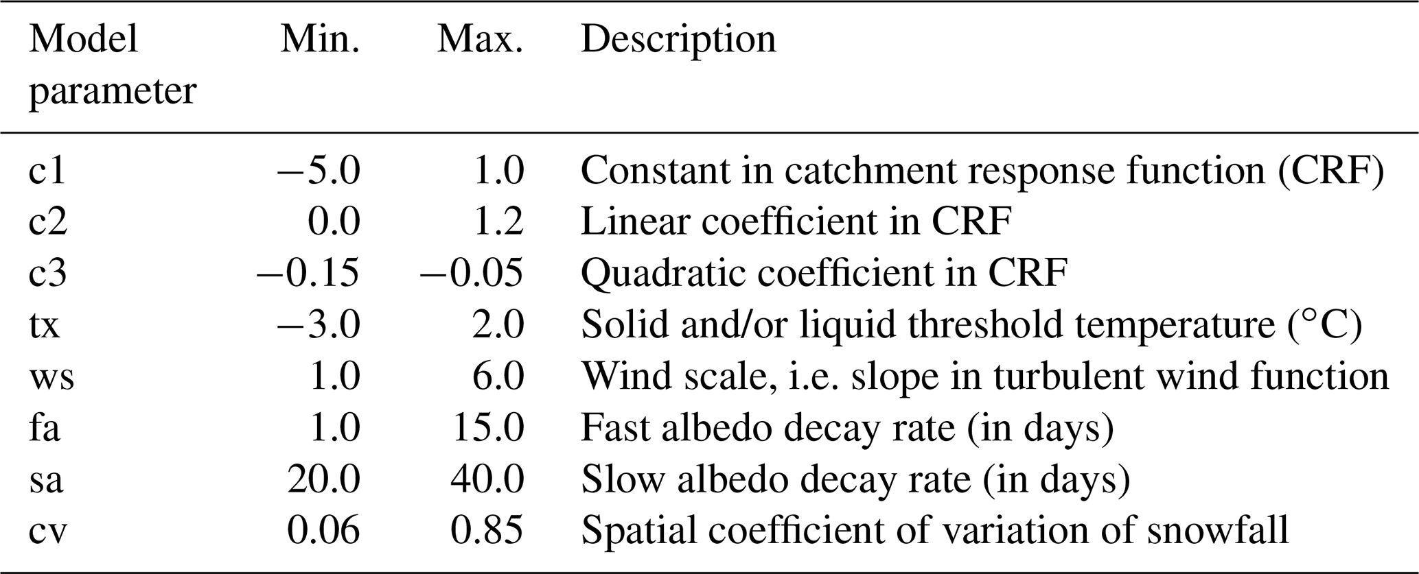
The Statkraft Hydrological Forecasting Toolbox, Shyft (https://shyft.readthedocs.io/en/latest/, last access: 18 September 2020), is an open-source distributed hydrological modelling framework developed by Statkraft (2018), with contributions from the University of Oslo and other institutions (e.g. Nyhus, 2017; Matt et al., 2018). The modelling framework has three main models (method stacks), and in this study the PT_GS_K model was used for the parameter identification study, using machine-learning-based emulators of the MC simulation. PT_GS_K is a conceptual hydrological model, and in this study eight of its parameters are subjected to uncertainty analysis. PT_GS_K uses the Priestley–Taylor (PT) method (Priestley and Taylor, 1972) to estimate potential evaporation; a quasi-physical-based method for snowmelt, sub-grid snow distribution, and mass balance calculations (GS method); and a simple storage–discharge function (Lambert, 1972; Kirchner, 2009) for catchment response calculations (K). Overall, these three methods constitute the PT_GS_K model in Shyft. The framework establishes a sequence of spatially distributed cells of arbitrary size and shape. As such, it can provide lumped (single cell) or discretized (spatially distributed) calculations as in this study. The modelling framework (Shyft), and the PT_GS_K model in particular, were described in previous studies (e.g. Burkhart et al., 2016; Teweldebrhan et al., 2018), and the reader is referred to these materials for further details on the underlying methods of this model. Table 2 shows a list of the uncertain model parameters and their parameter range.

Table 2 Range of model parameters used for the PT_GS_K model uncertainty analysis.

4.2 Study site and data

The data used to train and validate the ML emulators were retrieved from the Nea catchment. This catchment is located in the Sør-Trøndelag county, Norway (Fig. 3). The geographical location of the catchment ranges from 11.67390 to 12.46273^∘ E and from 62.77916 to 63.20405^∘ N. The Nea catchment covers a total area of 703 km², and it is characterized by a wide range of physiographic and land cover characteristics. Altitude of the catchment ranges from 1783 m above sea level (a.s.l.) on the eastern side, around the mountains of Storsylen, to 649 m a.s.l. at its outlet. The dominant land cover types in the catchment are moors, bogs, and some sparse vegetation, while a limited part of the catchment is forest covered (3 %). Mean annual precipitation for the hydrological years 2011–2014 was 1120 mm. The highest and lowest average daily temperature values for this period were 28 and −30 ^∘C, respectively.

Figure 3 Physiography and location map of the study domain.

The PT_GS_K model requires temperature, precipitation, radiation, relative humidity, and wind speed as forcing data. In this study, daily time series data of these variables were obtained from Statkraft (2018), with the exception of relative humidity. Daily gridded relative humidity data were retrieved from ERA-Interim (Dee et al., 2011). The model also requires the following physiographic data for each grid cell: average elevation, grid cell total area, and the areal fractions of forest, reservoir, lake, and glacier. Data for these physiographic variables were retrieved from two sources, namely the land cover data from Copernicus land monitoring service (2020) and the 10 m digital elevation model (10 m DEM) from the Norwegian mapping authority (2016). Daily observed streamflow measurements that were used in both behavioural model identification and validation that cover four hydrological years (1 September to 31 August) for the study area were also provided by Statkraft (2018).

5 Results

5.1 Evaluation of the MLMs' capability in reproducing the response surfaces

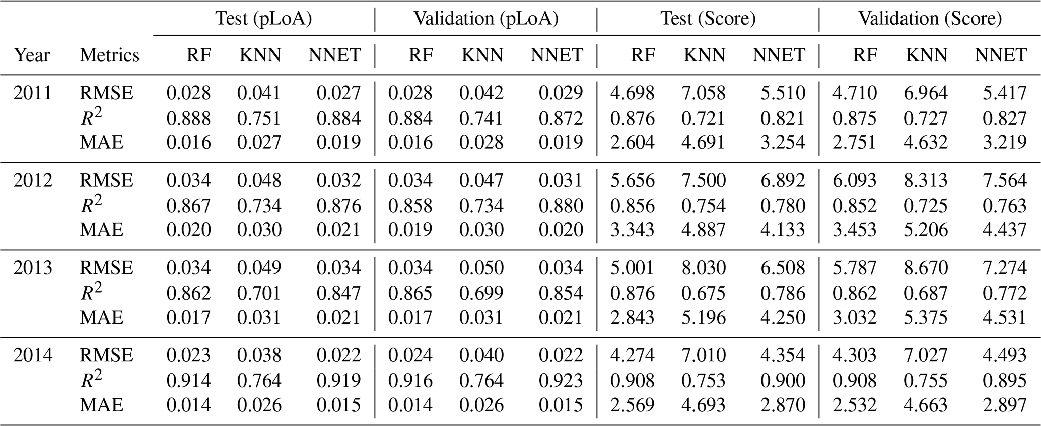
Table 3 shows the test and validation results of the MLMs trained to emulate the MC simulation. Two sets of MLM emulators were trained using the same covariates but different target variables, i.e. pLoA and Score. The pLoA and Score predicted using the test (S2) and validation (S3) samples were compared against their respective values estimated using the MC simulation. The evaluation metrics have shown variability both between the three MLMs and the analysis years. For the test samples and using pLoA as a target variable, a relatively lower performance was observed when using KNN, while similar results were obtained between RF and NNET. The highest performance of the MLMs was observed in year 2014, with R² values of 0.91, 0.76, and 0.92 for RF, KNN, and NNET, respectively, and the lowest performance was observed in year 2013 with R² values of 0.86, 0.7, and 0.85 for RF, KNN, and NNET, respectively. When using Score as a target variable and the test samples, RF, NNET, and KNN showed a decreasing order of performance based on the three evaluation metrics, i.e. RMSE, R², and MAE. The interannual comparison of the evaluation metrics shows that the relative performance of the MLMs, using Score as a target variable, was consistent throughout the 4 analysis years. Relative performances similar to the test samples were obtained for the validation samples for both MLMs_pLoA and MLMs_score. When it comes to the time efficiency of the emulators, they commonly take a few seconds to predict the response surface for the 95 000 samples, compared to over 24 h when running the Monte Carlo simulation for a single hydrological year.

Table 3 Evaluation results of the predicted target variables, i.e. pLoA (in fraction) and Score, through comparison against values estimated using the MC simulation for the test and validation samples.

5.2 Evaluation of behavioural parameter sets using observed streamflow

The behavioural model realizations identified using the coupled ML emulators and the limits of acceptability approach were evaluated using observed streamflow values. A cross-validation method was used to assess the performance of the model parameter sets identified in a given year through comparison of the simulated against observed streamflow values in the remaining years. The cross-validation result based on the streamflow efficiency measures used in this study, i.e. NSE and LnNSE, and the CR are depicted in Table 4. The behavioural model realizations performed very well both during the calibration and validation periods. During the calibration period, minimum NSE values of 0.81, 0.89, and 0.82 were, respectively, obtained for the models identified using RF, KNN, and NNET as emulators. Similarly, the maximum NSE values during this period were 0.93, 0.94, and 0.95, respectively, for RF, KNN, and NNET. The average NSE values for these emulators were 0.88, 0.91, and 0.88, respectively. During the validation period the value of NSE ranged 0.72–0.83, 0.66–0.85, and 0.71–0.83, respectively, for RF, KNN, and NNET. A relatively lower LnNSE value than NSE value was observed in most of the analysis years, with the exception of year 2012 where a relatively higher LnNSE than NSE was obtained when using RF and NNET during the calibration period. While a slightly higher average NSE was obtained when using KNN compared to RF and NNET during both calibration (0.91) and validation (0.85) periods, a slightly higher average LnNSE was obtained when using NNET during both calibration (0.85) and validation (0.79) periods.

Table 4 Cross-validation of the streamflow predictions of models identified using the coupled ML emulators and MC simulation. The efficiency metrics for the calibration period are shown in bold font.

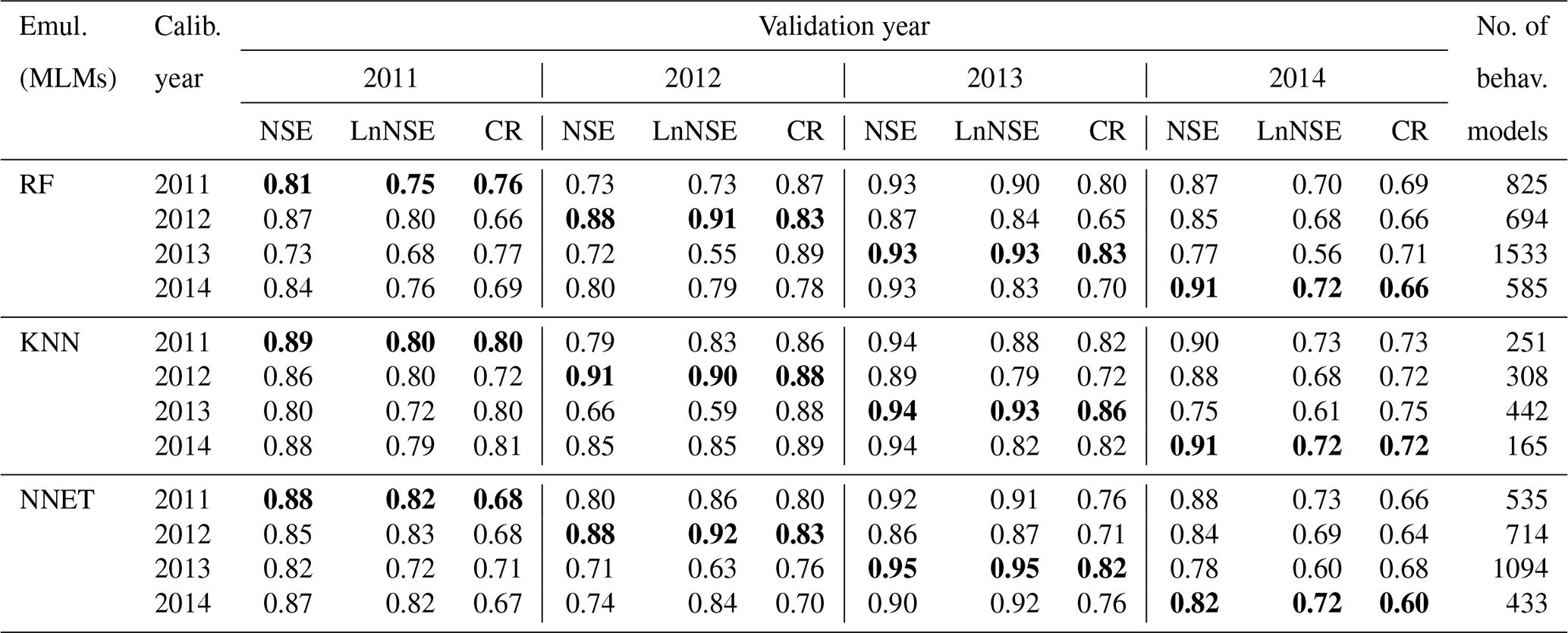
The measure of streamflow prediction uncertainty used in this study, i.e. CR, for the validation period has shown some variability based on the MLMs used in the behavioural model identification. When using RF, the highest and lowest CR values obtained were 0.65 and 0.89, respectively, with an overall mean value of 0.74. Similarly, minimum, maximum, and mean CR values, respectively, of 0.64, 0.80, and 0.71 were obtained when using NNET. The validation period CR values, when using KNN, ranged from 0.72 to 0.89, with an average value of 0.79, which is relatively higher compared to RF and NNET.

The interannual comparison between the three MLMs shows that the highest validation period average NSE (0.89) was obtained with the year 2014 as the calibration period and KNN as the ML emulator. Similarly, the highest average LnNSE (0.86) for the validation period was obtained when using models calibrated in the year 2014 but NNET as the ML emulator. On the other hand, the lowest average NSE (0.74) for the validation period was obtained when using the year 2013 as the calibration period and RF and KNN as the ML emulators. This shows that the models identified based on KNN were characterized by a relatively higher interannual variability in their performances (based on NSE) compared to those identified using RF and NNET. A relatively higher interannual variability in average CR (0.66 to 0.79) for the validation periods was obtained when using RF. The number of identified behavioural models has also shown an interannual variability for a given MLM and between MLMs within a given calibration year. The highest and lowest number of behavioural models was, respectively, obtained in calibration years 2013 and 2014. Similarly, the highest number of behavioural models was obtained when using RF, while the lowest record was obtained when using KNN.

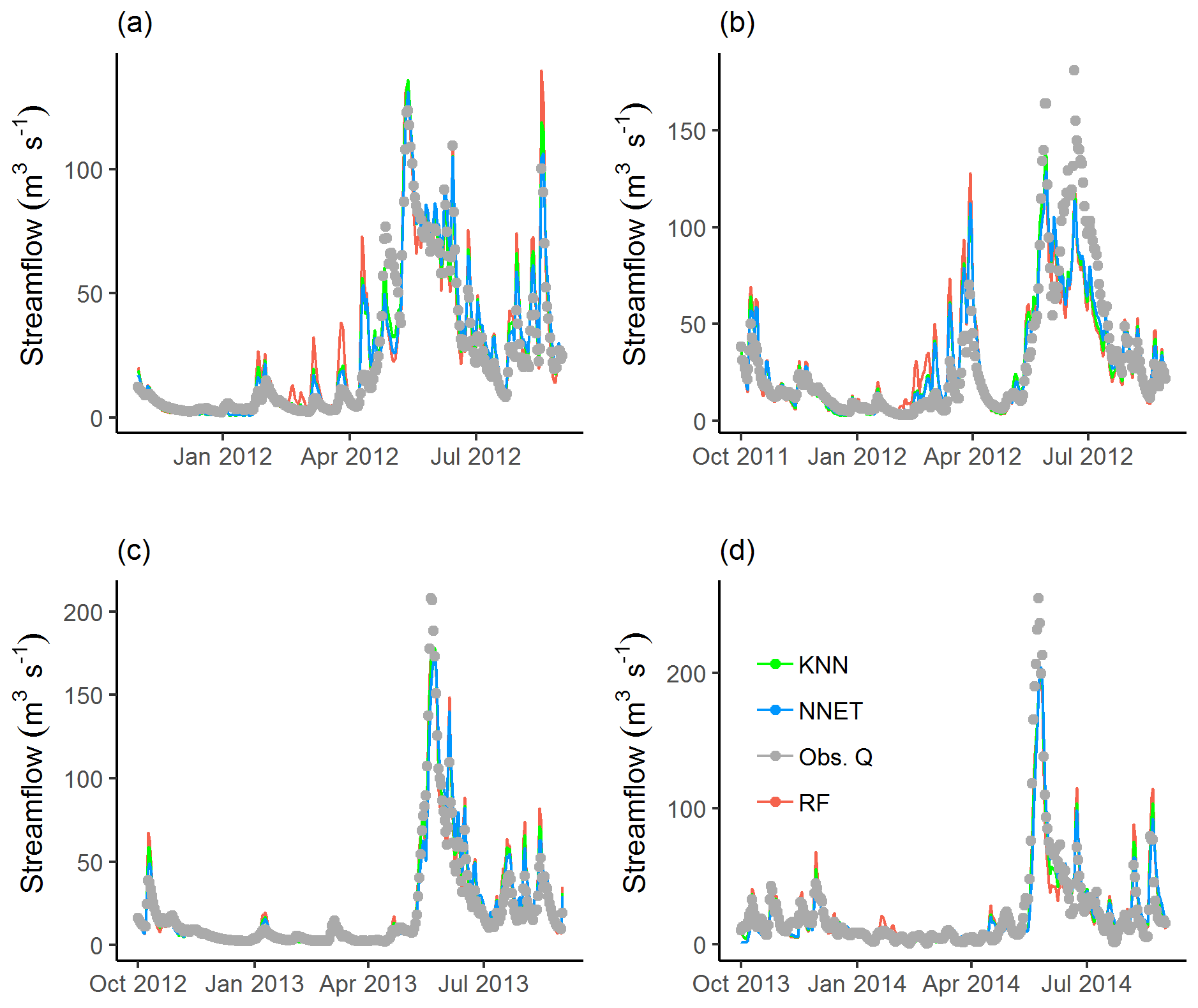
Figure 4 Simulated and observed streamflow values for the calibration period, i.e. year 2011 (a), and validation periods, i.e. years 2012 (b), 2013 (c), and 2014 (d). The behavioural models are identified using the coupled MLMs (RF, KNN, and NNET) and GLUE pLoA.

Figures 4 and 5, respectively, show the hydrographs and scatter plots of simulated against observed streamflow for a sample calibration period (year 2011) and validation periods (years 2012, 2013, and 2014). The streamflow predictions for the calibration period have shown a good fit with the observed values, with most of the predicted values falling close to the 1 : 1 identity line (dark line). However, some observations tend to be overestimated during the onset of snowmelt and underestimated during early summer flows (Fig. 4). Similarly, the small patch of the scatter points between 50 and 75 (m³ s⁻¹) of the observed values (Fig. 5) show underestimation for this streamflow range. This might be attributed to a poor estimation of the model parameters or due to an interaction of the model parameters that had a significant effect on the dominating processes in that flow range. In years 2012 and 2014, the predicted streamflow has shown a good fit with the low-flow observations. A mismatch was observed with the high-flow observations during the same period, where most of the high-flow observations are underestimated. These years are characterized by having the highest (year 2012) and lowest (year 2014) maximum snow water equivalent (data not shown) compared to the other years, and this may partly explain the observed low performance during the high-flow condition. The behavioural models identified using the three MLMs yielded very good streamflow predictions in year 2013. From the trend line fitted to the scatters, it can be noticed that the predictions based on RF tend to slightly underestimate for high-flow conditions and overestimate for low-flow conditions in years 2012 and 2014, compared to KNN and NNET. The later MLMs yielded fitted lines close to each other in both the calibration and validation periods, with the exception of year 2013 where KNN and NNET, respectively, yielded slightly over- and underestimated streamflow predictions for the high-flow condition.

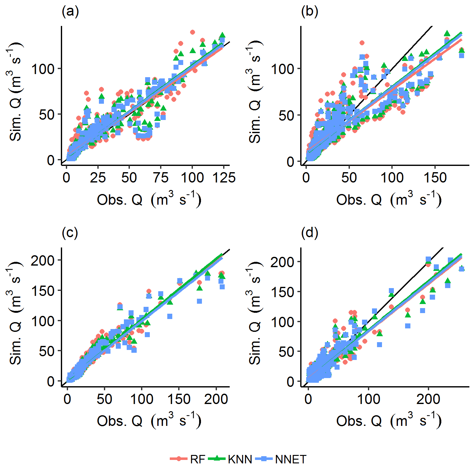
Figure 5 Scatter plots of simulated against observed streamflow values for the calibration period, i.e. year 2011 (a), and validation periods, i.e. years 2012 (b), 2013 (c), and 2014 (d).

The statistics summarizing the posterior model parameters identified with the help of the three MLMs (RF, KNN, and NNET) and those directly identified from the MC simulation (MC) are presented in Fig. 6. The result shows that the minimum values of c1 and c2 obtained from the three MLMs are similar to the calculated values. Comparable minimum values between the MLMs were also obtained for most of the other parameters, although with slight deviation from the MC estimated values for some of the parameters. For the other statistics, discrepancies were observed both within the MLMs and between the MLMs and MC estimated values. NNET has yielded similar snow coefficient of variation (cv) values to those estimated from the MC simulation for all quantiles. However, no consistent result was observed for most of the model parameters. While a certain MLM yields a closer quantile value to the calculated values in one parameter, it is superseded by another MLM in other parameters. A varying degree of distribution characteristics was also observed among the model parameters estimated by a given MLM. For example, c3 and ws have, respectively, shown highest negative and positive skews of −0.540 and 0.739 compared to the other parameters when using NNET (result not shown). In the GLUE methodology, the set of parameters is generally more important than the statistical characteristics of the individual parameters since different combinations of the model parameters may give similar results. For example, similar streamflow prediction efficiency criteria (NSE, LnNSE, and CR) were obtained during the calibration period of year 2012 when using models identified with the help of RF and NNET (Table 4).

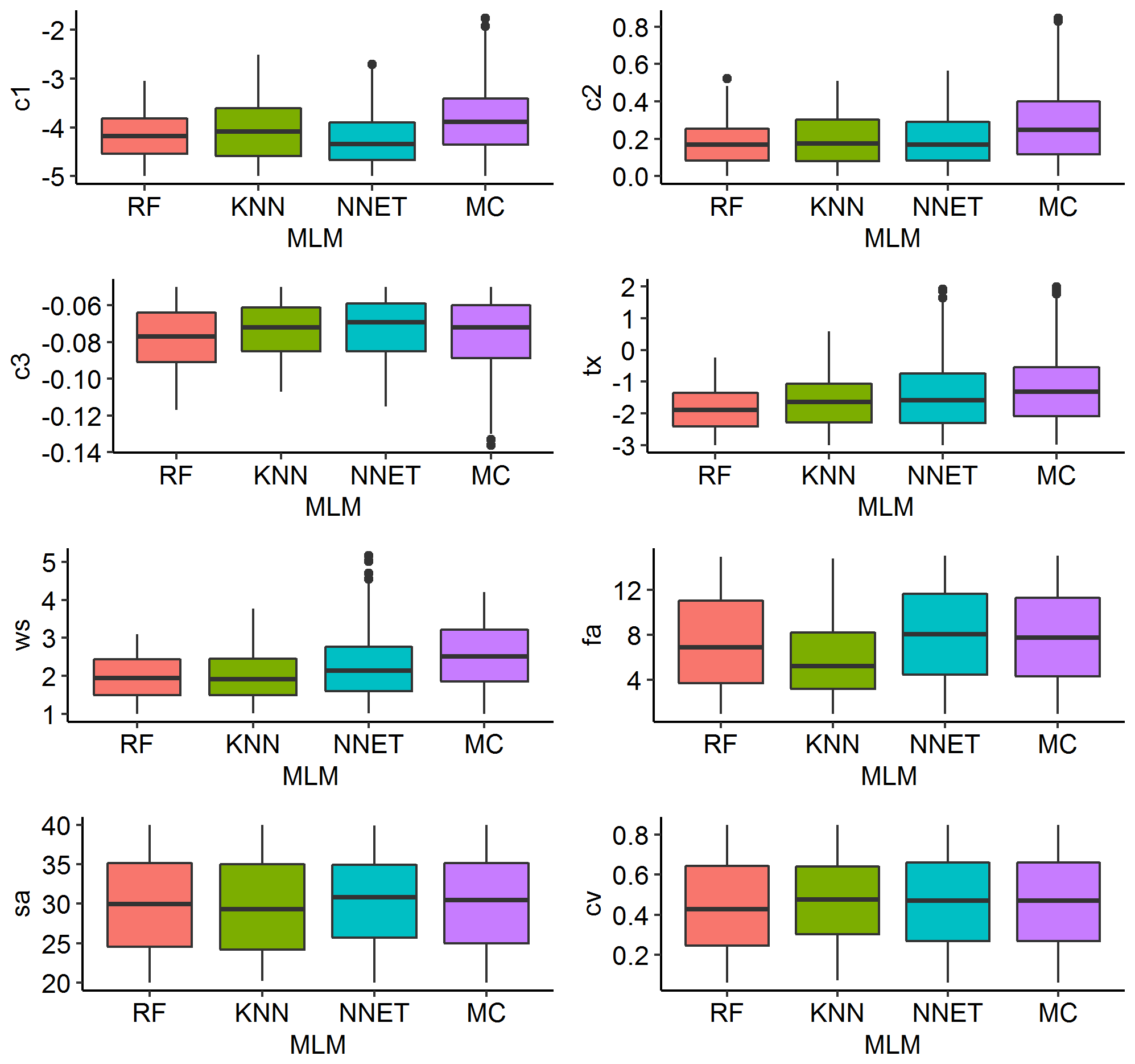
Figure 6 Posterior distribution plots of model parameters identified using the coupled MLMs and MC simulation (RF, KNN, and NNET) and those directly identified from the MC simulation (MC).

5.3 Variable importance and interaction

Sensitivity analysis is an important technique for assessing the robustness of model-based results, and it is often performed in tandem with emulation-based studies in order to determine which of the input parameters are more important in influencing the uncertainty in the model output (Ratto et al., 2012). Figure 7 shows the sensitivity of streamflow predictions to the model parameters based on the in-built variable importance assessment methods of the three MLMs trained to predict pLoA and Score. The relative measures of importance are scaled to have a maximum value of 100. The RF and KNN MLMs trained to predict pLoA yielded similar relative importance of the model parameters. The catchment response parameters of the hydrological model, viz. c1, c2, and c3, have shown higher relative importance compared to the snow and water balance parameters. On the other hand, the NNET trained to predict pLoA has yielded higher relative importance for wind scale (ws) and the rain and/or snow threshold temperature (tx) compared to the linear (c2) and quadratic (c3) coefficients of the catchment response function. The RF and KNN MLMs trained to predict Score have also shown similar results to their equivalent MLMs trained to predict pLoA, with the exception of a swipe in the order of importance between the two least important parameters, namely fa and cv, when using RF. The result from the NNET trained to predict Score was less consistent with the result obtained from its corresponding MLM trained to predict pLoA. The former result was similar to the one obtained from the KNN trained to predict Score, except that c3 was preceded by c1 and ws in the case of NNET. The snow coefficient of variation (cv) and the slow (sa) and fast (fa) albedo decay rates were the least important variables identified using the three MLMs when applied to predict pLoA and Score. The relative importance of the model parameters obtained using the MLMs was generally consistent with the result obtained in a previous study focused on parameter uncertainty analysis using the GLUE methodology (Teweldebrhan et al., 2018).

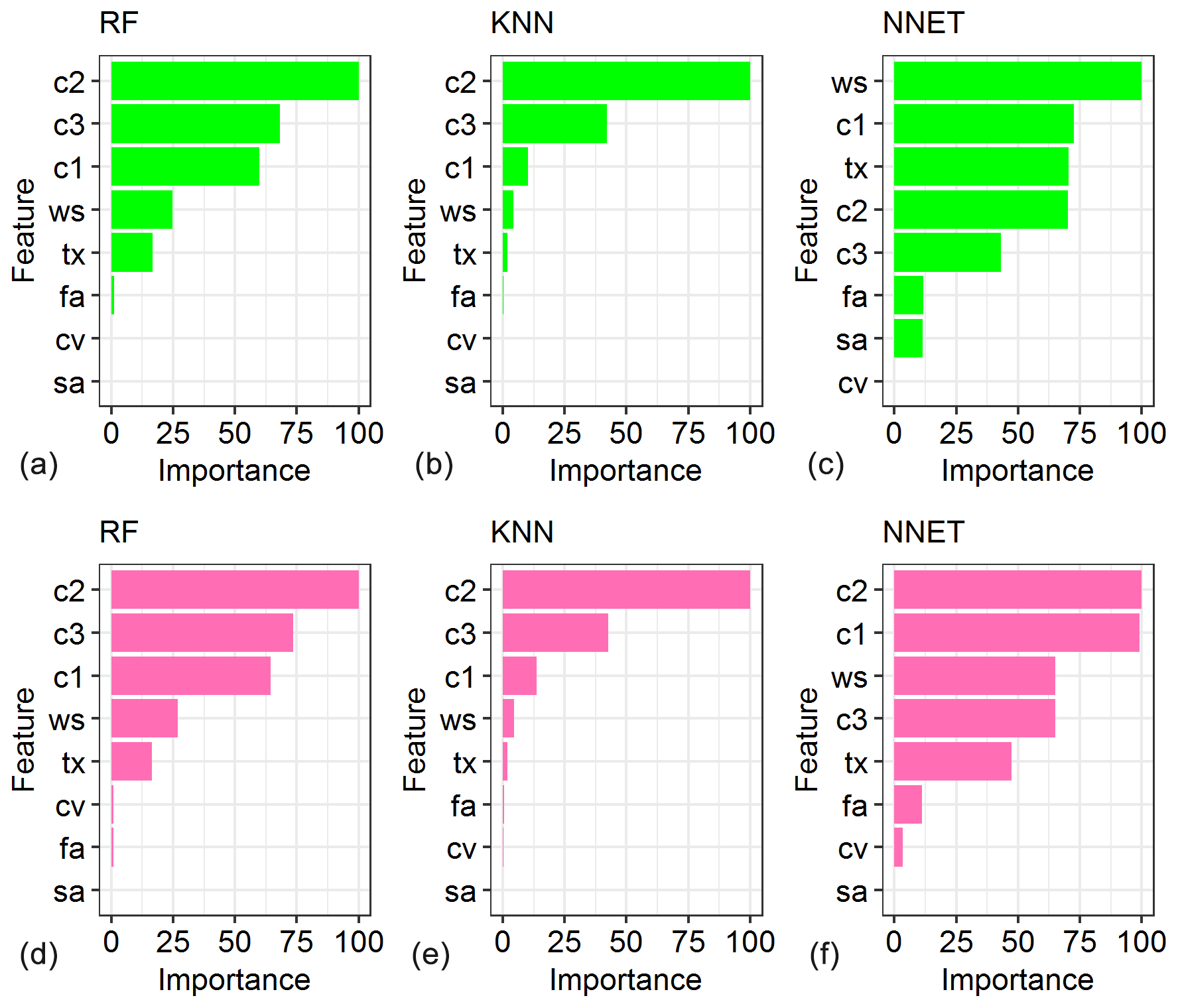
Figure 7 Relative importance of the hydrological model parameters based on the three machine-learning models, i.e. RF, KNN, and NNET, trained for pLoA (a–c) and Score (d–f).

Figure 8 presents a sample correlation matrix of the behavioural model parameters identified using the coupled RF as MLM and the MC simulation. The highest correlation was observed between tx and ws, with a Pearson correlation value of 0.57, followed by the correlation between c2 and c3, with a Pearson correlation value of 0.24. A correlation value of 0.22 was also obtained between c1 and ws. The high degree of interaction of ws with tx and c1 reveals that this parameter might have a significant effect on model results in combination with the other parameters, although it appears less important when considered alone.

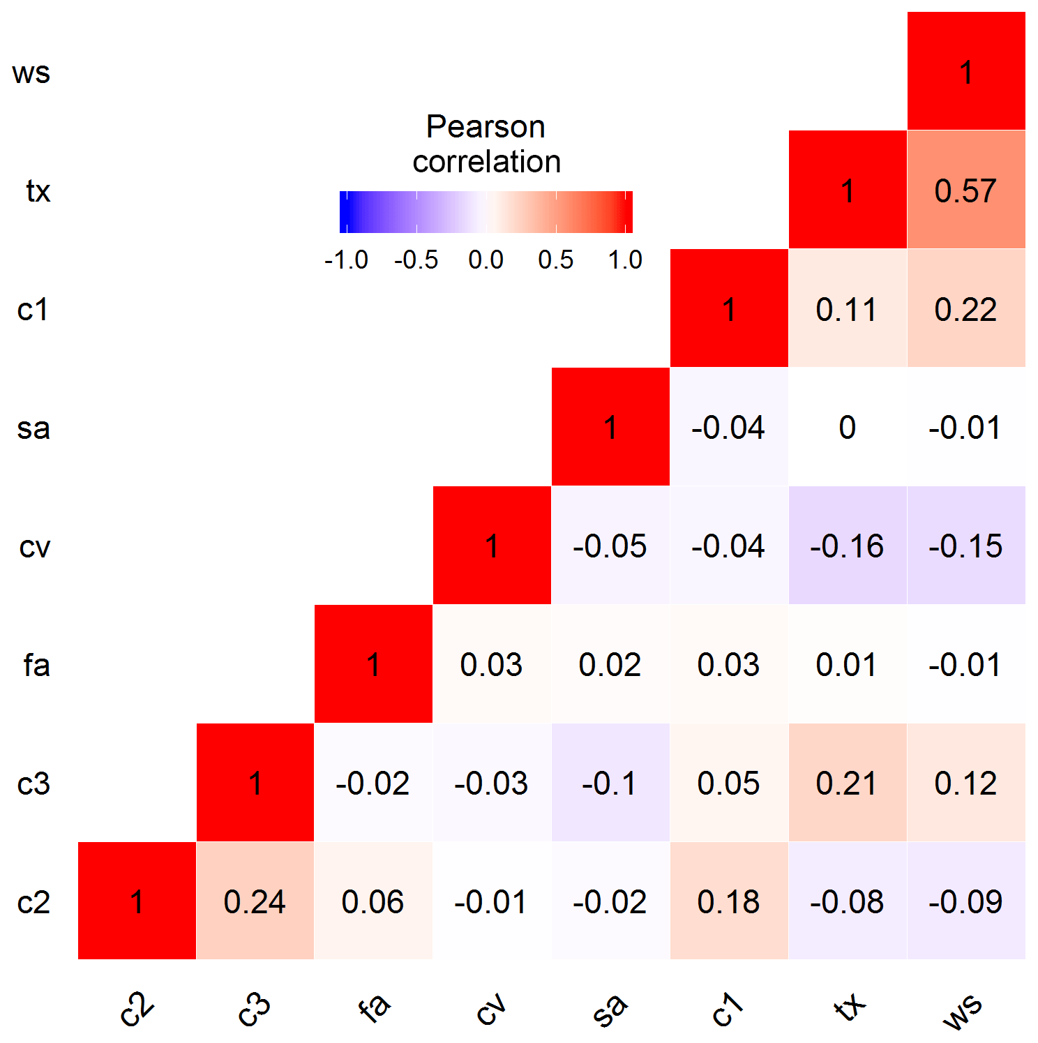
Figure 8 Pearson correlation matrix of the behavioural model parameters identified using the coupled RF and limits of acceptability approach.

6 Discussion

The capability of MLMs to act as emulators of the MC simulation has been demonstrated in this and other, similar studies. Machine-learning and other data-driven models have been applied as emulators to substitute complex and computationally intensive simulation models. These models have been referred to in the literature as surrogate models (e.g. Yu et al., 2015) and metamodels (e.g. El Tabach et al., 2007). Emulators were reported to be particularly useful when a large number of simulations, such as the MC simulation, is required to be performed, for example, during optimization (Hemker et al., 2008) and sensitivity analysis (e.g. Reichert et al., 2011). The results from this study revealed that the MLMs trained with a limited sample size of artificially generated data from the simulation model were computationally efficient and provided reliable approximations of the underlying hydrological system. Similar advantages of MLM-based emulators were also reported in previous studies (e.g. Kingston et al., 2018; Razavi et al., 2012).

The performance of the coupled MLMs in response to training sample size, however, varies from one MLM to another. For example, RF and KNN did not yield any behavioural models in some of the calibration years when the MLMs were trained with only 400 samples, while NNET yielded behavioural models in all years. Furthermore, the identified behavioural models, using the coupled MLMs with a limited sample size, had relatively low performances in reproducing the observed streamflow values. For example, NNET, KNN, and RF have, respectively, yielded an average NSE value of 0.73, 0.70, and 0.65 during the calibration period, which is generally lower than the respective values when using the training sample size of 4000. A further assessment of the sample size effect using 2000 training samples has shown only a slight decrease in the performance of the identified behavioural models (i.e. 1 %–3 % decrease in average NSE) compared to the ones identified using the 4000 samples. Only slight to no improvement was obtained in most of the evaluation years as a result of using behavioural models identified from the 4000 MC simulations, compared to the 95 000 simulations, when assessed using the available evaluation data set and the streamflow evaluation metrics used in this study. Like most studies based on the GLUE methodology, the main focus of this study was, however, to obtain as many behavioural models as possible so as to encapsulate future uncertain conditions.

The MLMs applied in this study and in other areas of application have both advantages and limitations. MLMs are able to learn a complex nonlinear system from a set of observations and usually yield a high degree of accuracy as they are not affected by the level of understanding of the underlying processes in the system (Kingston et al., 2018). Furthermore, MLMs with the virtue of their generalization capability are relatively quick to run as simulations over an extended period of time are not required. However, since MLMs do not have any understanding of the modelled physical processes, they operate as black box models with an accompanying dilemma on whether they would behave as intended under changing future conditions (Olden and Jackson, 2002). Generally, MLMs have limited applications in conditions that significantly deviate from historical norms. In this study, an adequate size of training samples was used in order to represent different parts of the parameter dimensions. Furthermore, in many MLMs the notion of degrees of freedom is usually ignored when computing performance metrics during model training (Kuhn, 2008). Since these metrics do not penalize model complexity (e.g. as in the case of adjusted R²), they tend to favour more complex fits over simpler models. In some MLMs a regularization approach is employed to adjust the cost function in such a way that the model learns slowly and, thereby, minimizes overfitting (Nielsen, 2018). In this study, for example, the L2 regularization was used with the NNET model.

In studies involving the use of the coupled ML and MC simulation, the uncertainty in parameter identification may stem from various sources. For example, the relative mismatch between the observed and simulated streamflow for the validation period in years 2012 and 2014, compared to the good fit in year 2013 (Fig. 5), can be attributed to the differences in hydrological conditions between the calibration and validation periods. Figure 9 shows the observed streamflow values of the 4 hydrological years at different percentiles. As can be noticed from this figure, the observed streamflow values for the validation period in year 2012 exceed those for the calibration period (year 2011) at all percentile values. On the other hand, streamflow recorded in year 2013 has shown closer values to those from year 2011 at most of the percentiles. The result from this analysis reveals that the identified model parameters yielded lower performances when applied to a hydrological condition that significantly deviated from the observations used for the identification of these parameters. This can be due to the prevalence of different dominant processes in different hydrological conditions.

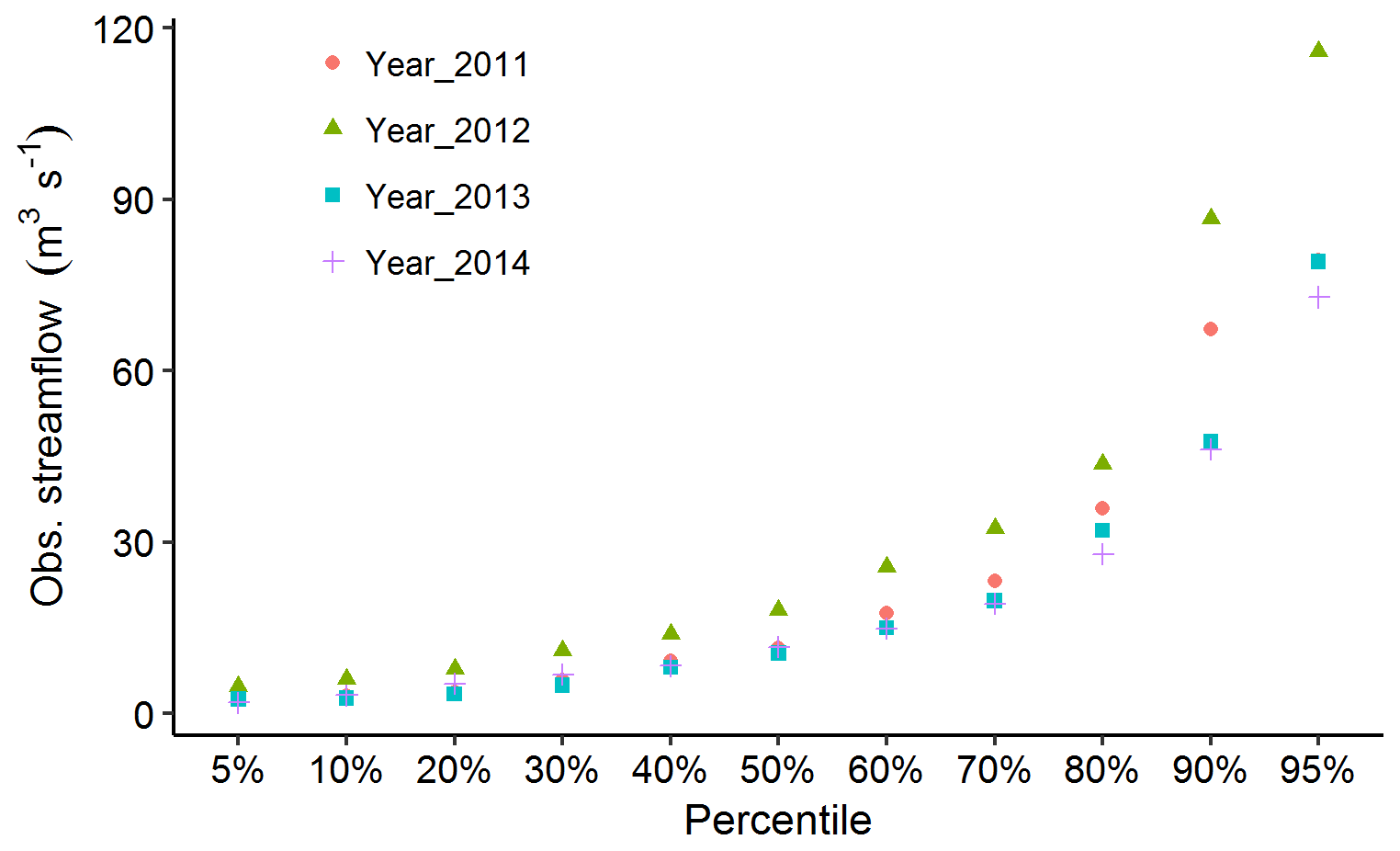
Figure 9 Comparison of the percentile of observed streamflow values for the calibration period (Year_2011) and validation periods (Year_2012, Year_2013, and Year_2014).

The highest average NSE and LnNSE values for the validation periods were obtained when using models identified in year 2012 and year 2014, respectively (Table 4). The Nash–Sutcliffe efficiency (NSE) computed using the row streamflow data gives more emphasis to high-flow than low-flow values, while the one computed using the log-transformed data (LnNSE) gives more emphasis to low-flow conditions. Thus, the models identified under the predominantly low-flow conditions, i.e. year 2014, were good at predicting low flows while those identified under high-flow conditions, i.e. year 2012, were good with the prediction of high flows when applied during the validation period. Generally, these phenomena are consistent with concerns raised in previous studies focused on the challenges of the model development philosophy based on a universal fixed model structure that is transposable in both space and time (e.g. Clark et al., 2011; Kavetski and Fenicia, 2011). The results from this study and other similar studies (e.g. Fenicia et al., 2011) suggest the need for additional components to emphasize dominant processes, although fixed model structures might be attractive due to their relatively parsimonious structure.

Although KNN was not a favourite emulator in previous hydrological studies, it has yielded a comparable result to the other MLMs used in this study. For example, the performance of KNN was superior to RF and NNET based on the average NSE obtained for the calibration period. However, the result from KNN was characterized by higher interannual variability compared to RF and NNET. Inconsistent relative performances between KNN and NNET were also reported in previous studies focused on flow forecasting using MLMs. For example, Wu and Chau (2010) obtained a better monthly streamflow forecast using KNN compared to NNET, although Mekanik et al. (2013) observed a better performance of NNET compared to KNN. A similar, inconsistent result was also observed in another study focused on monthly streamflow forecasting, with a higher cumulative ranking of NNET compared to KNN under nonlinear conditions (Modaresi et al., 2018). However, the latter was better at reproducing the observations under linear conditions; they concluded that the variability in the relative performance of the MLMs may be attributed to the differences between study sites, data sets, and structure of the MLMs as well as whether the relationship between the predictor and predicted variables is linear or nonlinear. The main challenges with KNN appear when data are sparse, although this problem can be partly overcome by choosing the number of neighbours adapted to the concentration of the data (Burba et al., 2009).

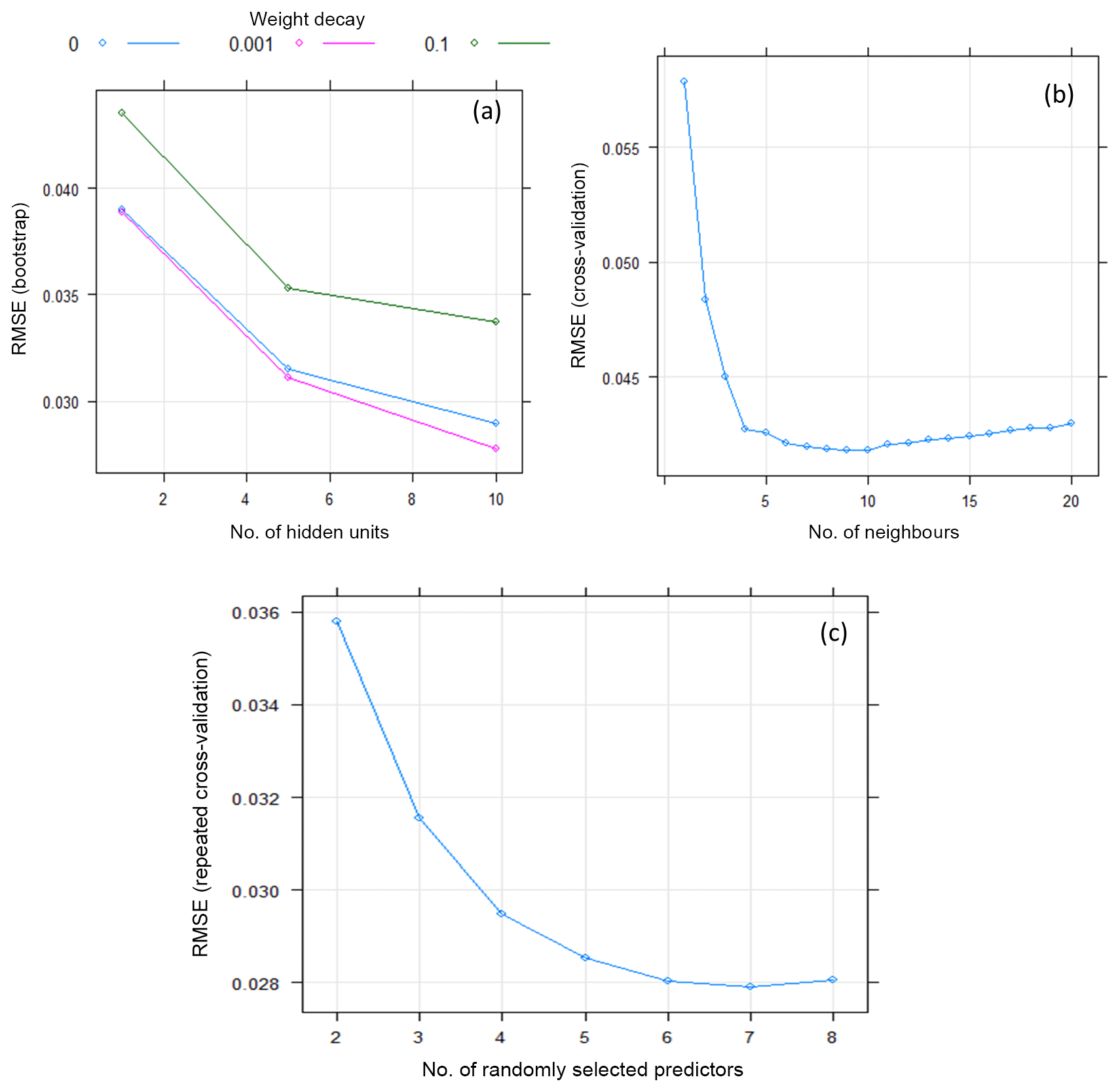
Figure 10 Bootstrap and cross-validation-based estimates of hyper-parameter values for the three machine-learning models, i.e. NNET (a), KNN (b), and RF (c), in a sample calibration period (year 2011).

In this study, different trials were conducted in order to assess the effects of the model structure and hyper-parameter values and, thereby, to obtain the optimal MLMs (result not shown). For example, the NNET model with multiple hidden layers resulted in a lower performance than the one with single hidden layer. This result is consistent with the general notion that, for many applications, a single hidden layer is adequate for modelling any nonlinear continuous function (e.g. Hsieh,2009; Snauffer, et al., 2018). Similarly, use of a linear activation function has yielded NNET models with better accuracy compared to the commonly used sigmoidal function. Efficiency of the emulators also depends on their respective hyper-parameters values. Figure 10 shows cross-validation and bootstrap analyses results when estimating the optimal hyper-parameter values of the machine-learning models using RMSE for a sample calibration period (year 2011). For NNET (Fig. 10a) two hyper-parameters were optimized using the training data set, i.e. the weight decay and number of neurons in the hidden layer (hidden units or size). The final values used for this model were a weight decay of 0.001 and hidden units of 10. For KNN (Fig. 10b), the optimal value of nearest neighbours (k) used for the final model was k=10; for the RF model (Fig. 10c), the optimal number of randomly selected predictors when forming each split (mtry) was 7.

In this study, the concept of equifinality was employed for parameter identification and uncertainty analysis, i.e. an ensemble of behavioural models were identified with subsequent application for streamflow prediction at different quantile values. In other studies focused on the concept of optimality, machine-learning methods were used to directly estimate prediction uncertainty based on MC-based uncertainty or historical model residuals from an optimal model. For example, in the machine learning in parameter uncertainty estimation (MLUE) method (Shrestha et al., 2009, 2014), MLMs were trained using MC-based uncertainty with a subsequent application of the trained MLMs to directly predict model output uncertainty associated with new input data sets. Similarly, clustering and machine-learning techniques were used to estimate the prediction uncertainty associated with a process model through analysis of its residuals during uncertainty estimation based on local errors and clustering (UNEEC; Solomatine and Shrestha, 2009). In a further study, the UNEEC approach was extended in a way that it could explicitly take parametric uncertainty into account (Pianosi et al., 2010). Similarly, Wani et al. (2017) have effectively applied instance-based learning, using KNN, in order to generate error distributions for predictions of an optimal model. Generally, the UNEEC and its variants are computationally more efficient than those based on the equifinality concept since, in the former case, only a single model run is required during the forecast period. Uncertainty analysis using emulators coupled to the residual-based GLUE is also expected to entail less computational cost compared to those coupled with GLUE LoA and its variants.

In previous emulator-based uncertainty analysis studies, the residual-based GLUE methodology was coupled with the MLMs (e.g. Yu et al., 2015). Here, we used the limits of acceptability concept in order to overcome some of the limitations associated with the residual-based approach. The original formulation of the GLUE LoA is, however, too strict for use in the identification of behavioural models, and it may result in the rejection of useful models and, thereby, make a type II error. In order to minimize such errors, one of the commonly used approaches was to relax the limits (e.g. Blazkova and Beven, 2009). However, in a previous study it was observed that relaxing the limits was not a feasible option in simulations that involve time series data with dynamic observational error characteristics as in the case of continuous rainfall–runoff modelling. Relaxing the limits beyond 25 %, while keeping the threshold pLoA at 100 %, has yielded the inclusion of nonbehavioural models, leading to very low performance during the validation period. Accordingly, in an attempt to find a balance between type I and type II errors, the time-relaxed limits of acceptability approach was introduced (Teweldebrhan et al., 2018). This approach was employed in this study, and it relaxes the strict criterion of the original formulation that demands that all model predictions fall within their respective observation error bounds. When using this approach, the minimum threshold for the percentage of time steps where model predictions are expected to fall within the limits is defined as a function of the level of modelling uncertainty.

A combined likelihood measure, based on the persistency of model realizations in reproducing the observations within the observational error bounds (pLoA) and a normalized absolute bias (Score), was used in a previous study focused on snow data assimilation (Teweldebrhan et al., 2019). The Score values were rescaled with due consideration to pLoA, whereby the two efficiency measures were given equal importance in estimating the final weight of each model. In this study, the acceptable models were first identified based on pLoA only, and Score was used to weigh the relative importance of the acceptable models in predicting the quantile streamflow values. Another trial that involved the selection of the top 100 best-performing models, using a combined likelihood with equal weights given to pLoA and Score, yielded relatively low validation results compared to using pLoA alone for the identification of behavioural models (result not shown). This can be attributed to the difference in nature of these likelihood measures. pLoA considers only the percentage of time steps where the model predictions have fallen within the observation error bounds. This renders pLoA less sensitive to the variability in relative performances of the model between time steps. On the other hand, Score can be highly affected by predictions of a few time steps that are very close or too far from the observed value, albeit within the limits. The predictability of independent variables varies from one to another. Thus, the application of emulation methods for predicting pLoA in this study provides further insight to the potential and scope of the standard emulator, i.e. NNET and the additional emulators used in this study, i.e. RF and KNN, for predicting response surfaces other than the residual-based likelihood measures that were applied in previous studies.

7 Conclusions

Three machine-learning models (MLMs), i.e. random forest (RF), K nearest neighbours (KNN), and an artificial neural network (NNET) were constructed to emulate the time-consuming MC simulation and, thereby, overcome its computational burden when identifying behavioural parameter sets for a distributed hydrological model. Two sets of MLMs were trained using the randomly generated uncertain model parameter values as covariates, and two efficiency criteria were defined within the realm of the limits of acceptability concept as target variables. One of the efficiency criteria used in this study was a measure of model persistency in reproducing the observations within the observation error bounds (pLoA), while the other one was based on a normalized absolute bias (Score). The coupled MLMs and time-relaxed limits of acceptability approach employed in this study were able to effectively identify behavioural parameter sets for the hydrological model. The MLMs were able to adequately reproduce the response surfaces for the test and validation samples with an R² value of 0.7 to 0.92 for the test data set, although the evaluation metrics have shown variability between both the MLMs and the analysis years. RF and NNET yielded comparable results (especially for pLoA), while KNN has shown a relatively lower result. Capability of the MLMs to act as emulators of the MC simulation was further evaluated through comparison of streamflow predictions using the identified behavioural model realizations against the observed streamflow values. The identified behavioural models have performed very well in reproducing the median streamflow prediction during both the calibration and validation periods, with an average NSE value of 0.89 and 0.83, respectively. The cross-validation result also shows that the high-flow conditions, as measured by average NSE, were slightly better estimated under both the calibration and validation periods when KNN was used as an emulator, compared to RF and NNET, while NNET yielded a slightly better prediction under low-flow conditions (LnNSE). Although the behavioural models identified based on KNN have shown a relatively higher interannual variability, they have yielded comparable performances to RF and NNET in terms of the efficiency measures. Future studies may assess the possibility of using the three MLMs as ensemble emulators to obtain an improvement in the identification of behavioural parameter sets while significantly minimizing the computational burden of the MC simulation.

The sensitivity analysis conducted using the in-built algorithms of the three MLMs has yielded a comparable order of precedence in relative variable importance when trained using pLoA and Score as target variables. The result was generally consistent with the one obtained from a previous study conducted using the residual-based GLUE methodology. The catchment response parameters of the hydrological model, i.e. c1, c2, and c3, have shown higher relative importance compared to the snow and water balance parameters. Thus, the efficiency of MLM-based emulators in doing sensitivity analysis for computationally expensive models was also further proven in this study.