the Creative Commons Attribution 4.0 License.
the Creative Commons Attribution 4.0 License.
 | 04 Sep 2020
Assessment of meteorological extremes using a synoptic weather generator and a downscaling model based on analogues
Damien Raynaud
Benoit Hingray
Anne-Catherine Favre
Jérémy Chardon
Natural risk studies such as flood risk assessments require long series of weather variables. As an alternative to observed series, which have a limited length, these data can be provided by weather generators. Among the large variety of existing ones, resampling methods based on analogues have the advantage of guaranteeing the physical consistency between local weather variables at each time step. However, they cannot generate values of predictands exceeding the range of observed values. Moreover, the length of the simulated series is typically limited to the length of the synoptic meteorological records used to characterize the large-scale atmospheric configuration of the generation day. To overcome these limitations, the stochastic weather generator proposed in this study combines two sampling approaches based on atmospheric analogues: (1) a synoptic weather generator in a first step, which recombines days of the 20th century to generate a 1000-year sequence of new atmospheric trajectories, and (2) a stochastic downscaling model in a second step applied to these atmospheric trajectories, in order to simulate long time series of daily regional precipitation and temperature. The method is applied to daily time series of mean areal precipitation and temperature in Switzerland. It is shown that the climatological characteristics of observed precipitation and temperature are adequately reproduced. It also improves the reproduction of extreme precipitation values, overcoming previous limitations of standard analogue-based weather generators.
- Article
(5581 KB) - Full-text XML
- BibTeX
- EndNote


Increasing the resilience of socio-economic systems to natural hazards and identifying the required adaptations is one of today's challenges. To achieve such a goal, one must have an accurate description of both past and current climate conditions. The climate system is a complex machine which is known to fluctuate at very small timescales but also at large ones over multiple decades or centuries (Beck et al., 2007). It is necessary to study meteorological series as long as possible in order to catch all sources of variability and fully cover the large panel of possible meteorological situations. Regarding weather extremes, the same need arises, as estimating return levels associated with large return periods cannot be successfully done without long climatic records (e.g. Moberg et al., 2006; Van den Besserlaar et al., 2013). This comment also applies to all statistical analyses on any derived variable, such as river discharge, for which multiple meteorological drivers come into play and for which extreme events correspond to the combination of very specific and atypical hydro-meteorological conditions.
Using weather generators, long simulations of weather variables provide accurate descriptions of the climate system and can be used for natural hazard assessments. Among the large panel of existing weather generators, stochastic ones are used to construct, via a stochastic generation process, single or multi-site time series of predictands (e.g. precipitation and temperature) based on the distributional properties of observed data. These characteristics, and consequently the weather generator parametrization, are usually determined on a monthly or seasonal basis to take seasonality into account. They can also be estimated for different families of atmospheric circulation, often referred to as weather types. The state of the art of the most common methods which have been used for the downscaling of precipitation (single or multi-site) is presented in Wilks and Wilby (1999) and in Maraun et al. (2010). More recent publications gather detailed reviews of some sub-categories of weather generators (e.g. Ailliot et al., 2015, for hierarchical models). An increasing number of studies focus on the generation of multi-variate and/or multi-site series of predictands (e.g. Steinschneider and Brown, 2013; Srivastav and Simonovic, 2015; Evin et al., 2018a, b). Stochastic weather generators are able to produce large ensembles of weather time series presenting a wide diversity of multi-scale weather events. For all these reasons, they have been used for a long time to enlighten the sensitivity and possible vulnerabilities of socio-ecosystems to the climate variability (Orlowsky and Seneviratne, 2010) and to weather extremes.
Other models used for the generation of weather sequences are based on the analogue method. Since the description of the concept of analogy by Lorenz (1969), the analogue method has gained popularity over time for climate or weather downscaling. This analogue-model strategy has been applied in many studies (Boé et al., 2007; Abatzoglou and Brown, 2012; Steinschneider and Brown, 2013) and has been used to address a wide range of questions from past hydro-climatic variability (e.g. Kuentz et al., 2015; Caillouet et al., 2016) to future hydro-meteorological scenarios (e.g. Lafaysse et al., 2014; Dayon et al., 2015). The standard analogue-approach hypothesizes that local weather parameters are steered by synoptic meteorology. A set of relevant large-scale atmospheric predictors is used to describe synoptic weather conditions. From the atmospheric state vector, characterizing the synoptic weather of the target simulation day, atmospheric analogues of the current simulation day are identified in the available climate archive. Then, the analogue method makes the assumption that similar large-scale atmospheric conditions have the same effects on local weather. The local or regional weather configuration of one of the analogue days is then used as a weather scenario for the current simulation day. The key element of the analogue method is that it does not require any assumption on the probability distributions of predictands. This is a noteworthy advantage for predictands, such as precipitation, which have a non-normal distribution with a mass in zero. Most of the studies using analogues focused on precipitation and temperature either for meteorological analysis (Chardon, 2014; Ben Daoud et al., 2016) or as inputs for hydrological simulations (Marty et al., 2013; Surmaini et al., 2015). Nevertheless, analogues are increasingly used for other local variables such as wind, humidity (Casanueva et al., 2014) or even more complex indices (e.g. for wild fire; Abatzoglou and Brown, 2012). When multiple variables are to be downscaled simultaneously, another major advantage of the analogue method is that the different predictands scenarios are physically consistent and the simulated weather variables are bound to reproduce the correlations between the variables (e.g. Raynaud et al., 2017) and sites (Chardon et al., 2014). Indeed, when analogue models use the same set of predictors (atmospheric variables and analogy domains) for all predictands, all surface weather variables and sites are sampled simultaneously from the historical records, thus preserving inter-site and inter-variable dependency.
The two simulation approaches (stochastic weather generators and analogue methods) described above present some important advantages for the generation of long weather series but also some sizable drawbacks. Indeed, stochastic weather generators rely on strong assumptions about the statistical distributions of predictands. Identifying the relevant mathematical representations of the processes and achieving a robust estimation of their parameters can be difficult, especially if the length of the meteorological records is short. Modelling the spatial–temporal dependency between variables and sites is often another challenge. Conversely, for the analogue-based approaches, the identification of relevant atmospheric variables providing good prediction skills is not straightforward. The limited length of local weather records is also a critical issue, since resampling past observations restricts the range of predicted values. In particular, the simulation of unobserved values of predictands is not possible. This can be problematic if one is interested in estimating possible extreme values of the considered variable. Furthermore, the information on synoptic atmospheric conditions required by analogue methods are generally coming from atmospheric reanalyses, which also have a limited temporal coverage (e.g. from the beginning of the 20th century for ERA-20C – EMCWF Reanalysis; Poli et al., 2016) and from the mid-19th century for 20CR (Twentieth Century Reanalysis; Compo et al., 2011). The length of the generated time series is thus typically bounded by the length of the reanalyses.
In this study we propose a weather generator (hereafter SCAMP+) building upon the SCAMP (Sequential Constructive atmospheric Analogs for Multivariate weather Prediction) approach presented by Chardon et al. (2018) and making use of reshuffled atmospheric trajectories, following some of the developments by Buishand and Brandsma (2001) and Yiou (2014). With the weather scenarios generated by SCAMP being limited by the coverage of the climate reanalyses, the SCAMP+ model extends the pool of possible atmospheric trajectories. Using random transitions between past atmospheric sequences, SCAMP+ generates unobserved atmospheric trajectories on which the two-stage SCAMP approach can be applied. By exploring a wide variety of atmospheric trajectories, SCAMP+ introduces some additional large-scale variability which improves the exploration of possible weather sequences. In addition, as done in SCAMP (Chardon et al., 2018), the SCAMP+ approach includes a simple stochastic weather generator which is estimated, for each generation day, from the nearest atmospheric analogues of this day. These two steps (random atmospheric trajectories and random daily precipitation and temperature values) improve the reproduction of extreme values, overcoming previous limitations of analogue-based weather generators, usually known to underestimate observed precipitation extremes.
These developments are carried out for the exploration of hydrological extremes (extreme floods) of the Aare River basin in Switzerland (Andres et al., 2019a, b). Meteorological forcings, i.e. temperature and precipitation, are thus simulated to be used as inputs of a hydrological model, for different sub-basins of the Aare River basin. Meteorological simulations from SCAMP+ have been used in the Swiss EXAR (Hazard information for extreme flood events on the rivers Aare and Rhine) project1 and have proven its ability to estimate the discharge values associated with very large return periods on the Aare River. In Sect. 2, we describe in details the test region, the data and three simulation approaches (a classical analogue method, referred to as ANALOGUE, SCAMP and SCAMP+). Section 3 presents the main results of both climatological characteristics and extreme values. Section 4 sums up the main outputs of this study and proposes some further developments and analysis.
2.1 Studied region
This study is carried out on the Aare River basin, which covers almost half of Switzerland (17 700 km2). The topography varies greatly within the basin with, on one hand, high mountains on its southern part (maximum altitude of 4270 m, Finsteraarhorn) and on the other hand, plains on the northern part (minimum altitude of 310 m). These different characteristics coupled with the basin are located at the crossroads of several climatic European influences give a wide diversity of possible weather situations across the year.
2.2 Atmospheric reanalysis and local weather data
The application of the analogue method requires a long archive providing an accurate description of both past synoptic weather patterns and local atmospheric conditions. Indeed, a wide panel of meteorological situations available for resampling is necessary in order to identify the best analogues for the simulation (e.g. Van Den Dool et al., 1994; Horton et al., 2017). In most studies, synoptic situations are provided by atmospheric reanalyses. Here, we use the ERA-20C atmospheric reanalysis (Poli et al., 2013), which provides information on large-scale atmospheric patterns on a 6 h basis from 1900 to 2010. Data are available at a 1.25∘ spatial resolution. More specifically, the set of predictors used for the identification of atmospheric analogues is made of the geopotential height at 500 and 1000 hPa, the vertical velocities at 600 hPa, large-scale precipitation, and temperature. The justification of these choices will be given in Sect. 3.3.1.
The local and surface weather parameters of interest are retrieved from 105 weather stations for precipitation and 26 weather stations for temperature, which are spread out homogeneously over our target region, as presented in Fig. 1. These data are available at a daily time step from 1930 to 2014. They have been spatially aggregated in order to obtain daily time series of mean areal precipitation (MAP) and temperature (MAT) for the Aare region. The three weather generators considered in this study aim at producing scenarios of daily time series of MAP and MAT. In this study, a scenario is defined as a possible realization of the climate system under current climate conditions (i.e. the climate observed for the past few decades). It can be noticed that many applications of analogue-based approaches produce simulations at specific weather stations. However, as shown by Chardon et al. (2016) for France, the prediction skill is significantly improved when the prediction is produced for areal averages, which motivates the generation of MAP and MAT values in this study.
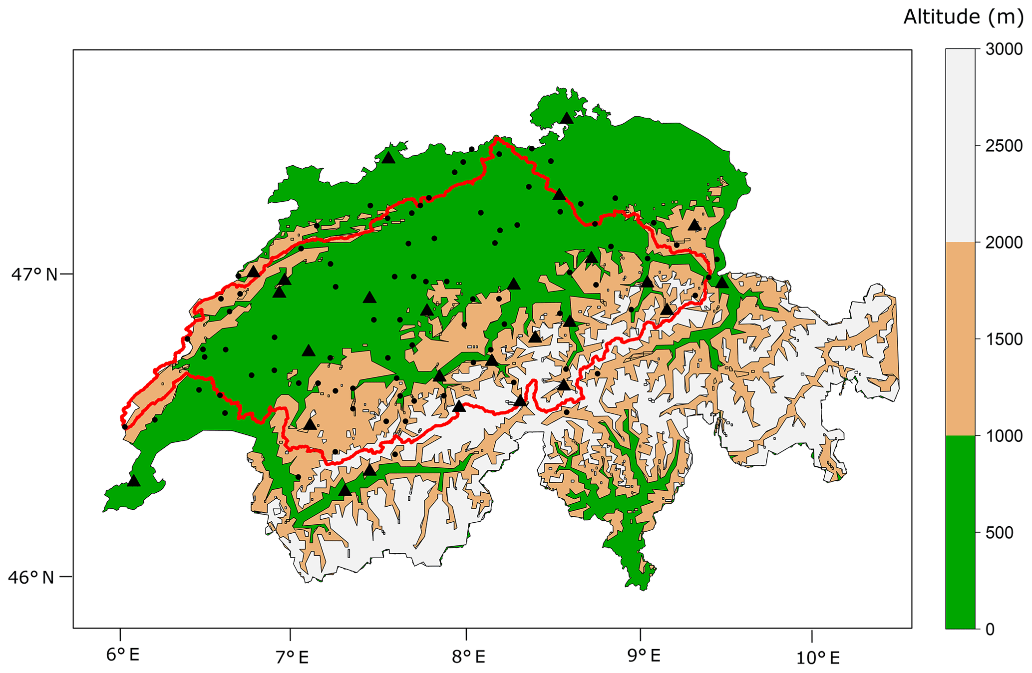
Figure 1The Aare River basin (red) and locations of the different precipitation (dots) and temperature (triangles) stations.
2.3 Description of the three models
This section presents the three different models considered and evaluated in this study.
2.3.1 ANALOGUE: classical analogue model
The most basic model evaluated in this study, hereafter referred to as ANALOGUE, relies on a standard two-level analogue method. For each day of the simulation period (1900–2010), analogue days are identified from candidate days. The candidate days extracted from the archive period, i.e. the period during which both predictors and local observations are available (1930–2010), are all days of the archive located within a 61 d calendar window centred on the target day. This calendar filter is expected to account for the possible seasonality of the large-scale–small-scale downscaling relationship. For instance, candidate days for 15 May 2000 are selected within the pool of days ranging from 15 April to 14 June of each year of the archive.
The predictors used for the analogue selection were chosen based on Raynaud et al. (2017). They have been shown to guarantee both inter-variable physical consistency and good predictive skills according to the Continuous Ranked Probability Skill Score (CRPSS) for four predictands (precipitation, temperature, solar radiation and wind). In the present work, the predictors considered for each level for the two-level analogy are as follows:
-
The first level of analogy is based on daily geopotential heights at 1000 and 500 hPa (HGT1000 and HGT500) as proposed by Horton et al. (2012) and Raynaud et al. (2017). The analogy criterion used here is the Teweles–Wobus score (TWS) proposed by Teweles and Wobus (1954). This score has been found to lead to higher performance than a more classical Euclidian or Mahalanobis distance (Kendall et al., 1983; Guilbaud and Obled, 1998; Wetterhall et al., 2005). It quantifies the similarity between two geopotential fields by comparing their spatial gradients. It allows for selecting dates that have the most similar spatial patterns in terms of atmospheric circulation. From September to May, the analogy is based on the geopotential fields on both the current day D and its following day D+1 at 12:00 UTC. Thereby, the motions of low-pressure systems and fronts are better described, and the prediction skill of the method for precipitation is improved (e.g. Obled et al., 2002; Horton and Brönnimann, 2019). In summer, only the geopotential fields on the current day are used as no similar improvement could be found with a 2 d analogy. During this first analogy level, 100 analogues are selected for each day of the target period.
-
The second analogy level makes a sub-selection of 30 analogues within the 100 analogues identified in the first analogy level. The analogy score used for the selection is the root mean square error (RMSE). From September to May, the predictors are the vertical velocities at 600 hPa and the large-scale temperature at 2 m. In summer, not only the vertical velocities but also other predictors such as the convective available potential energy (CAPE) led to a rather poor prediction of precipitation due to the coarse resolution of the atmospheric reanalysis, which prevents it from providing an accurate simulation of convective processes. Consequently, large-scale precipitation from the reanalysis has been used as a predictor instead, resulting in predictive skills similar to the ones obtained for the rest of the year. The different predictor sets retained for summer and the rest of the year illustrate the differences typically observed between seasons for the main meteorological conditions and processes.
The dimensions and position of the different analogy windows used to compute the analogy measures are presented in Fig. 2. They follow the recommendations for the analogy windows optimization presented in Raynaud et al. (2017) for all predictors.

Figure 2Positions and dimensions of the analogy windows in the analogue model at both analogy levels. Z500: geopotential at 500 hPa; Z1000: geopotential at 1000 hPa; VV600: vertical velocities at 600 hPa; P: precipitation; T: temperature.
With this two-step analogy, 30 scenarios of daily MAP and daily MAT are obtained for each day of the simulation period (1900–2010). Combined with the Schaake shuffle method described in Sect. 3.3.4, the application of the ANALOGUE model leads to 30 scenarios of 110-year time series of daily MAP and MAT.
2.3.2 SCAMP: combined analogue and generation of MAP and MAT values
The SCAMP model enhances the previous ANALOGUE approach, which is not able to generate daily values exceeding the range of observed precipitation and temperature. SCAMP combines the analogue method with a day-to-day adaptive and tailored downscaling method using daily distribution adjustment (Chardon et al., 2018).
For each prediction day, the following discrete–continuous probability distribution proposed by Stern and Coe (1984) is fitted to the 30 MAP values obtained from the atmospheric analogues of this day:
where π is the precipitation occurrence probability and FGA is the gamma distribution parameterized with a shape parameter α>0 and a rate parameter β>0. The π parameter is directly estimated by the proportion of dry days, and the parameters α and β of the gamma distribution are estimated by applying the maximum likelihood method to the positive precipitation intensities among the 30 MAP values. Thirty MAP values are then sampled from the distribution model defined in Eq. (1) in order to obtain unobserved values of precipitation, possibly beyond past observations. When there are less than five positive MAP intensities in the analogues, we simply retrieve the MAP analogue values. This distribution model corresponds to a simplified version of the combined analogue and regression model described in Chardon et al. (2018), and we refer the reader to this paper for further information.
Similarly, for each prediction day, a Gaussian distribution FN(μσ) is fitted to the 30 MAT values obtained from the analogues. A sample of 30 new MAT values is then generated from this fitted Gaussian distribution.
As for the ANALOGUE approach, the Schaake shuffle reordering method is applied to the daily scenarios obtained from SCAMP. A total of 30 scenarios of 110-year time series of daily MAP and MAT are produced.
2.3.3 SCAMP+
As mentioned previously, the first limitation of the analogue method is related to the length of the synoptic weather information that is used to generate local predictand time series. In the present case, the length of time series that can be produced with the models ANALOGUE and SCAMP is limited to 110-year-long weather scenarios.
In SCAMP+, we extend the archive of synoptic weather information by rearranging the synoptic weather sequences, thus creating new atmospheric trajectories, used in turn as inputs to SCAMP. This generation of new trajectories makes use of atmospheric analogues, following those of the principles proposed in the weather generators described by Buishand and Brandsma (2001) and Yiou (2014). For any given day, the atmospheric synoptic weather is considered to have the possibility to change its trajectory. The main hypothesis of this generation module is that if days J and K are close atmospheric analogues with atmospheric patterns heading in the same direction, then their “future” is exchangeable, and one could jump from one atmospheric trajectory to the other. In other words, day J+1 is a possible future of day K, and conversely day K+1 is a possible future of day J. The probability p to jump from one trajectory to any other is considered as a parameter to estimate.
The principle of a random atmospheric-trajectory generation is sketched on Fig. 3. In the present work, the only predictor involved with comparing the synoptic atmospheric configuration between 2 different days is the geopotential height field at 1000 hPa, for both the present day and its followers. The spatial analogy domain is the one used in Philipp et al. (2010) for the identification of Swiss weather types. The first line of Fig. 3 presents an observed atmospheric trajectory in HGT1000 from 8–12 February 1934. On 9 February, we look for analogues of the current day and its following day D+1. This is done to ensure that the two initial states are similar (high-pressure system located over France on 9 February 1934 and on its analogue, 28 January 1921) and that the main features move in similar directions (high-pressure system heading southeast on both 10 February 1934 and 29 January 1921).
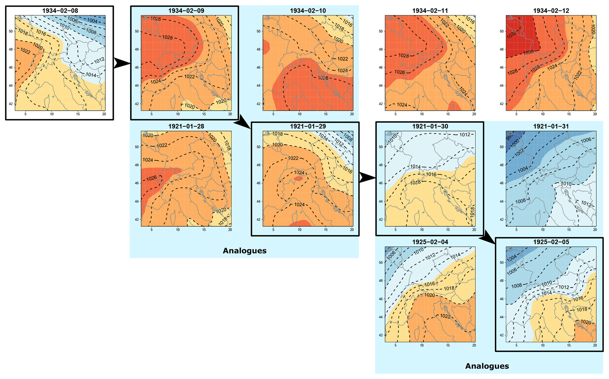
Figure 3Construction of a new 5 d atmospheric trajectory from an observed synoptic weather sequence. Each panel presents the geopotential at 1000 hPa on the domain of interest. The black squares and arrows give the new atmospheric trajectory, and the blue shading highlights the 2 d analogue that helps the “changing of atmospheric direction”.
Practically, the five best analogues of the current atmospheric 2 d sequence are identified, and one of those sequences is then selected with a probability p to generate the new day of the new trajectory. The same method is repeated for this new day to find its future day (as illustrated in Fig. 3 for the sequence 30 January 1921–12 February 1925) and extend the new trajectory by 1 additional day. This process is repeated as long as necessary. In the present work, it was used to generate a 1000-year trajectory of daily synoptic weather situations. Rather large differences between the synoptic weather situation can be obtained after some days between the observed atmospheric sequence (e.g. 12 February 1934) and the random atmospheric trajectory (12 February 1925). As we will show later on, such a method leads to higher weather variability at multiple timescales.
To ensure that 2 consecutive days of the generated sequences belong to the appropriate season, the five 2 d analogue sequences are identified within a ±15 d moving window centred on the calendar day of the target simulation day (e.g. all June days if the target day is xxxx-06-15 in the year-month-day date format).
The transition probability p from one observed trajectory to another indirectly determines the level of persistency of synoptic configurations. In this study, it has been calibrated in order to guarantee a good climatology of the large-scale atmospheric sequences. To do so, we analysed the mean frequency and duration of each of the nine weather types proposed for Switzerland by Philipp et al. (2010) in the observed synoptic series and in different reconstructed ones for transition probability p ranging from 1∕10 (one transition every 10 d on average) to 1 (one transition every day on average). The results presented in Fig. 4 show that a transition probability of 1∕7 is necessary to generate atmospheric trajectories that present a relevant persistency within each weather type.
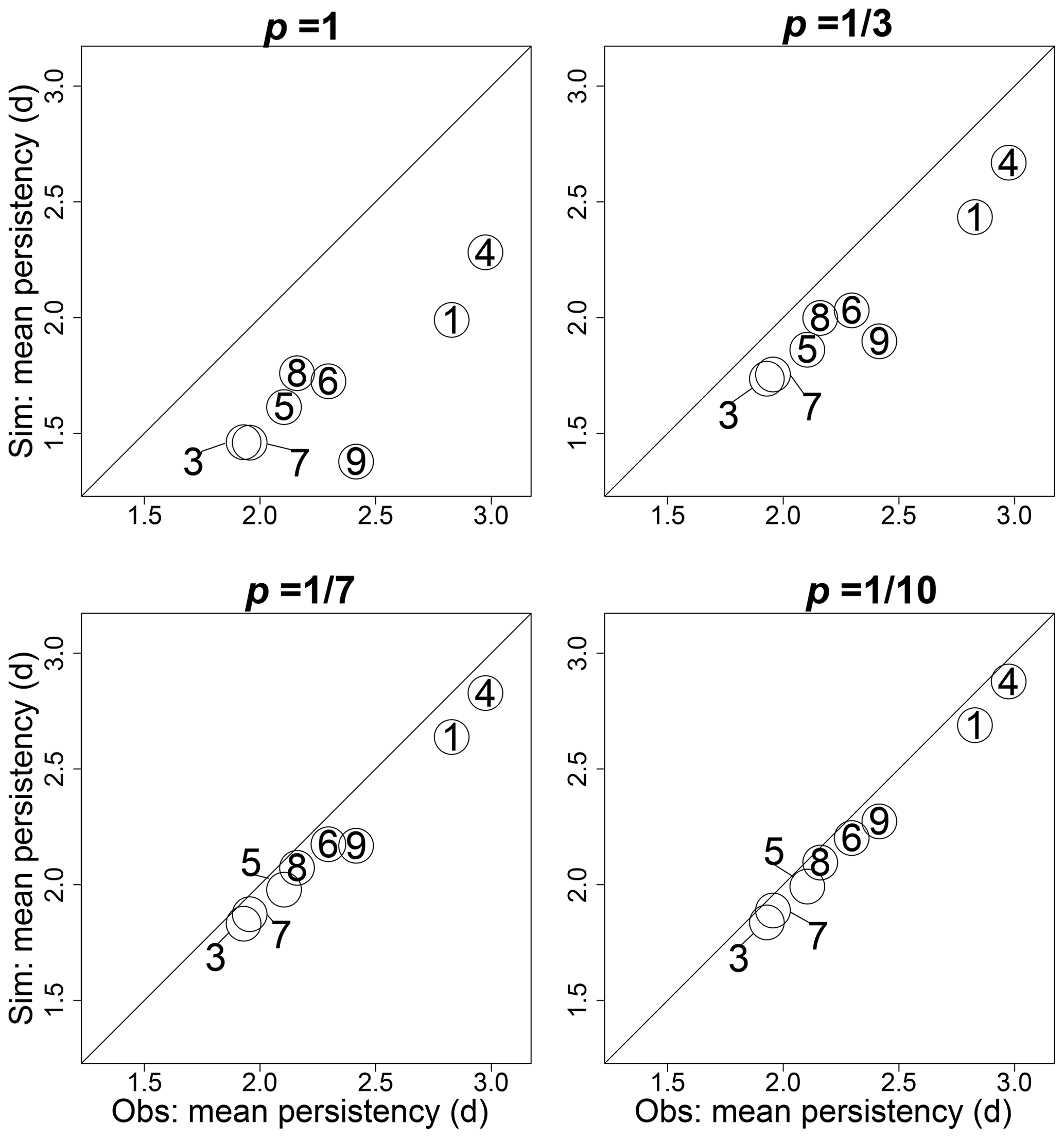
Figure 4Mean persistency (in days) of each of the nine weather types (indicated by the different circles in each panel), as defined by Philipp et al. (2010), in the observed time series and in the simulated ones for transition probabilities ranging from 1 to 1∕10 for the generation of atmospheric trajectories.
The long time series of synoptic weather generated with the above approach is further used as inputs to the SCAMP generator described in the previous section. The SCAMP+ approach leads to 30 scenarios of daily MAP and MAT, each of these scenarios being based on the 1000-year random atmospheric-trajectory sequence. The output of this approach, combined with the Schaake shuffle method described in the next section, is thus composed of 30 scenarios of 1000-year time series of daily MAP and MAT.
2.3.4 Temporal consistency: application of the Schaake shuffle
For each model (ANALOGUE, SCAMP and SCAMP+) and each day of the simulation period, 30 scenarios of daily MAP and MAT are produced. To improve the temporal and physical consistency between 2 consecutive days or between the temperature and precipitation scenarios (partially induced by the synoptic weather series), we use the Schaake shuffle method initially proposed by Clark et al. (2004). This method makes use of both the inter-variable physical and the intra-variable temporal consistency in observations to combine, at best, the outputs of any weather generator and reconstruct consistent predictand time series. It is particularly useful if one is interested in generating relevant precipitation accumulation scenarios over several days. A full description of the Schaake shuffle method can be found in Clark et al. (2004), and some applications can be found in Bellier et al. (2017) and in Schefzik (2016). Here, the Schaake shuffle consists in modifying the sequences of MAP and MAT values, preserving the association of the ranks of MAP and MAT, and rearranging sequences between days D and D+1. Shuffled MAP and MAT sequences between consecutive days then have similar associations than what has been observed. In this study, we give priority to the temporal consistency of precipitation first. Temperature scenarios are recombined in a second step.
The different components of the models ANALOGUE, SCAMP and SCAMP+ are summarized in Fig. 5.
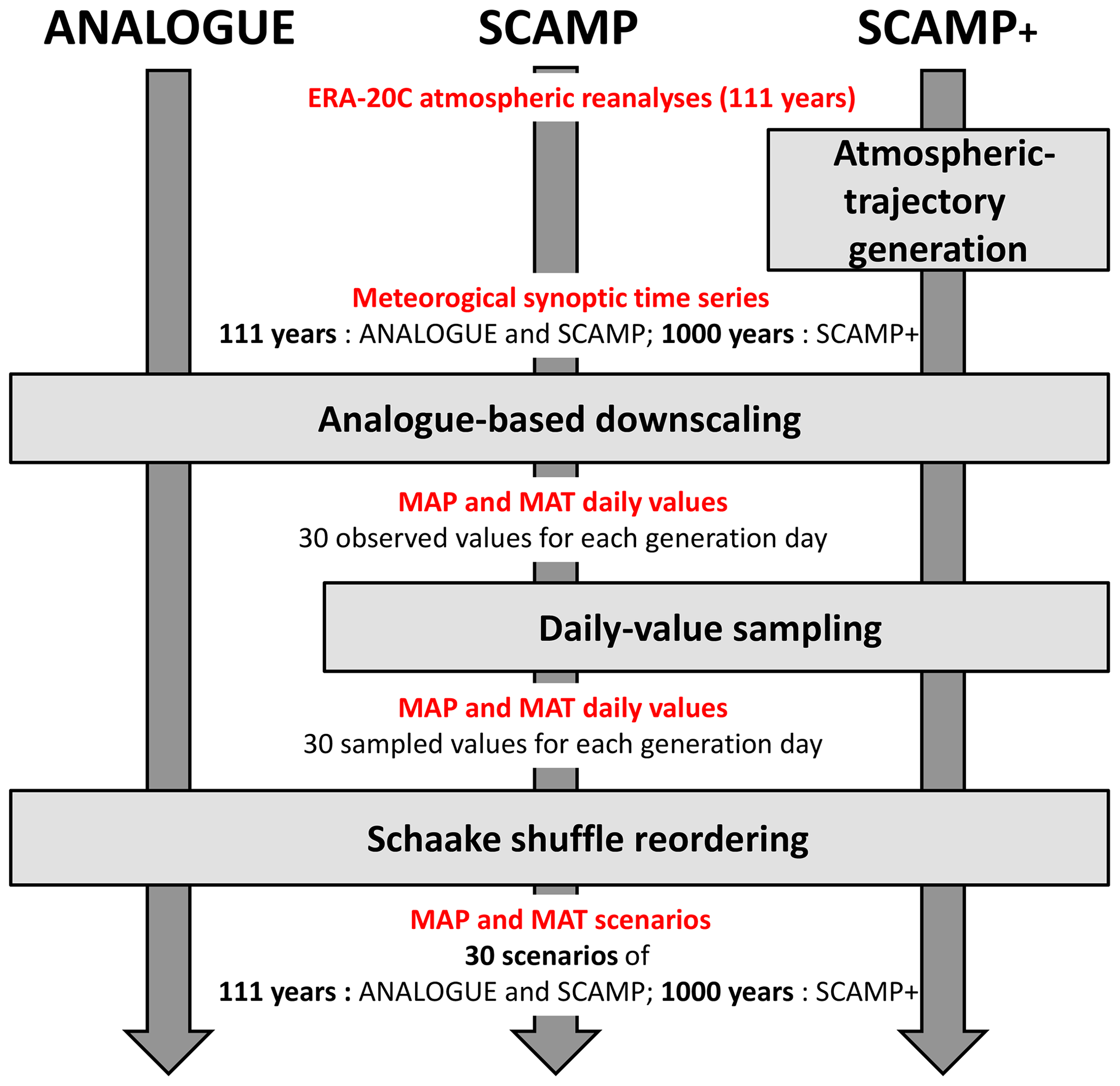
Figure 5Illustration of the different steps applied (grey boxes) with models ANALOGUE, SCAMP and SCAMP+. Outputs obtained after each step are indicated in red.
This section presents different statistical properties of the scenarios obtained with the three models and discusses the performances of each model by comparison with observed statistical properties. For the sake of consistency between the outputs, we compare the 30 scenarios of 111 years obtained from ANALOGUE and SCAMP to 300 scenarios of 100 years from SCAMP+ (i.e. each scenario of 1000 years is divided into 10 scenarios of 100 years).
3.1 Climatology
For both temperature and precipitation, the three models lead to an accurate simulation of their seasonal fluctuations (Fig. 6). However, one can notice the slight overestimation of winter temperature and an underestimation of July and August precipitation. SCAMP also tends to have a smaller inter-annual variability compared to ANALOGUE and SCAMP+.

Figure 6Observed and simulated seasonal cycles of temperature and precipitation for ANALOGUE, SCAMP and SCAMP+. The grey shadings present the inter-quantile intervals at 50 %, 90 % and 99 % levels. Simulated seasonal cycles are obtained using 30 scenarios of 111 years from ANALOGUE and SCAMP and 300 scenarios of 100 years from SCAMP+.
The distributions of seasonal precipitation amounts and seasonal temperature averages are presented in Fig. 7. Whatever the season, the three models are able to generate drier and wetter seasons than the observed ones (Fig. 7a). The very similar results obtained for ANALOGUE and SCAMP suggest that the daily distribution adjustments used in SCAMP do not introduce more variability at the seasonal scale. SCAMP+ is able to generate seasonal values that significantly exceed the maximum values simulated by ANALOGUE and SCAMP (by 100 to 200 mm). This strongly suggests that a large part of the seasonal variability comes from the variability of the synoptic weather trajectories, the unobserved weather trajectories produced by SCAMP+ leading to a wider exploration of extreme seasonal values.
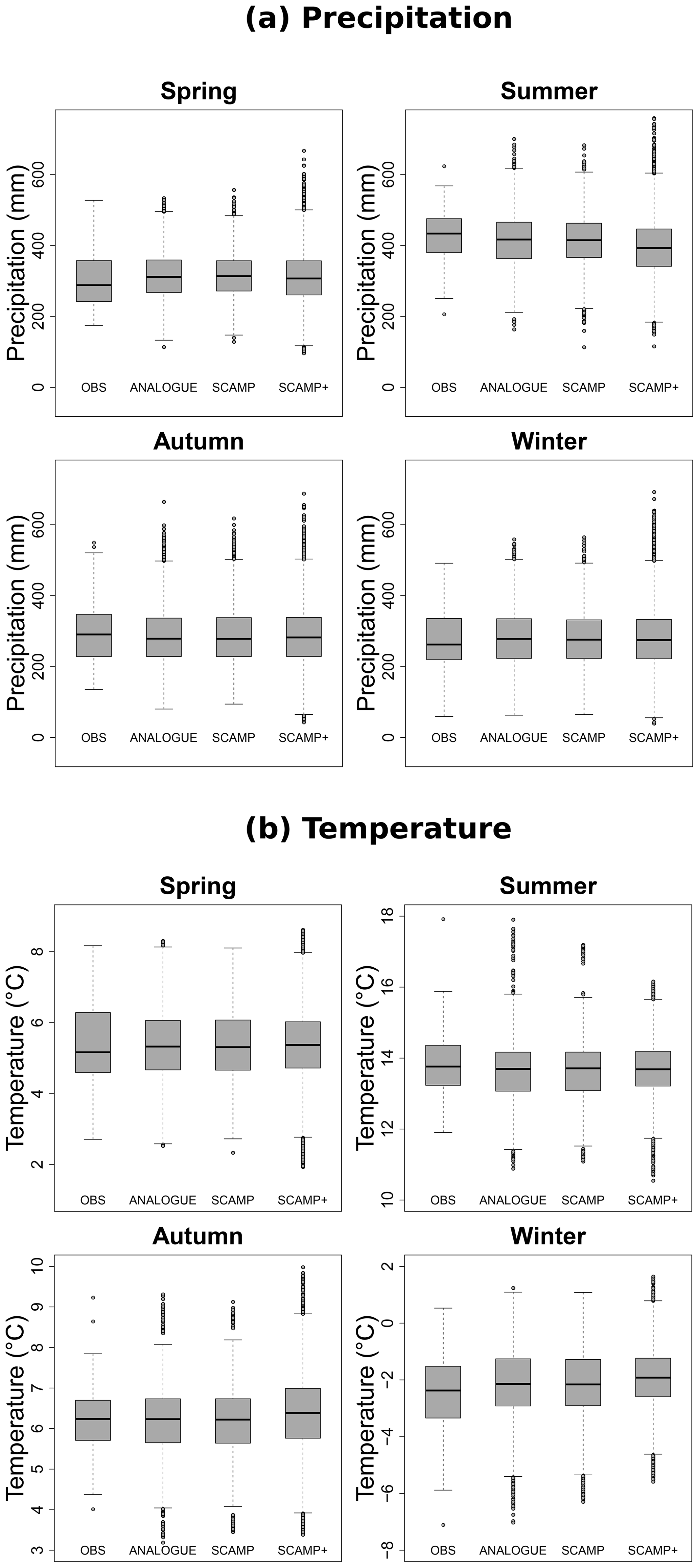
Figure 7(a) Observed and simulated boxplots of seasonal precipitation amounts for ANALOGUE, SCAMP and SCAMP+ (spring: March, April, May; summer: June, July, August; autumn: September, October, November; winter: December, January, February). (b) Observed and simulated boxplots of mean seasonal temperature for models ANALOGUE, SCAMP and SCAMP+ (spring: March, April, May; summer: June, July, August; autumn: September, October, November; winter: December, January, February).
The same comments can be made for spring and autumn temperatures (Fig. 7b). For those variables however, SCAMP+ fails to simulate extremely hot summers or cold winters. This limitation will be further discussed in the next section with some additional analysis and opportunities for improvement.
3.2 Daily precipitation extremes
As mentioned in Sect. 1, simple analogue methods cannot simulate unobserved precipitation extremes at the temporal resolution of the simulation (here daily). Moreover, for higher aggregation durations, they also tend to underestimate observed precipitation extremes. Figure 8 presents the precipitation values obtained with the three models for different return periods (from 2 to 200 years) and different aggregation durations (from 1 to 5 d).
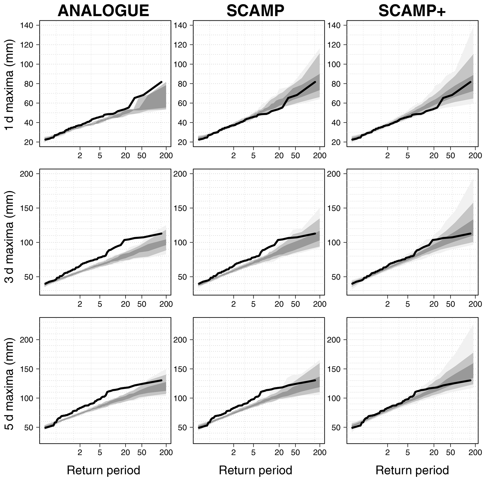
Figure 8Return level analysis of extreme precipitation values associated with models ANALOGUE, SCAMP and SCAMP+ for accumulation over 1, 3 and 5 d. The grey shadings present the inter-quantile intervals at 50 %, 90 % and 99 % levels (30×111-year scenarios for models ANALOGUE and SCAMP and 300×100-year scenarios for SCAMP+).
Considering 1 d extreme events, ANALOGUE is obviously not able to generate precipitation accumulations that exceed the maximum observed one. Combining the analogue method with daily distribution adjustments (SCAMP) overcomes this issue with maximum values reaching 115 mm. SCAMP+ leads to similar results.
The large underestimation of daily extremes obtained with ANALOGUE leads to an important underestimation of 3 and 5 d extremes. Despite a better simulation of daily values, SCAMP does not improve significantly the reproduction of 3 and 5 d extremes. SCAMP+ outperforms both models for all durations and generates precipitation extremes in agreement with observed extremes. Whatever the return period, the variability between the different 100-year scenarios is larger with SCAMP than with ANALOGUE and much larger with SCAMP+. This again suggests that 3 to 5 d extreme events can arise from atypical synoptic conditions, possibly not available in a 110-year long weather archive. Thanks to the random atmospheric trajectories, SCAMP+ is able to generate such conditions.
3.3 Multi-annual variability
Figure 9a and b presents examples of simulated time series of annual MAP and MAT obtained with ANALOGUE and SCAMP models. Concerning SCAMP+, four (among the 10 possible scenarios) illustrative time series associated with different 100-year atmospheric trajectories are shown. For all models, we present the dispersion between the 30 annual values obtained from the 30 time series associated with the different atmospheric trajectories. This dispersion is very small for temperature and rather large in comparison for precipitation, illustrating the important uncertainty in the large-scale–small-scale relationship for this variable in this region.

Figure 9(a) Time series of annual MAP for the ANALOGUE model (1900–2010), SCAMP (1900–2010) and four different 100-year atmospheric trajectories (t1, t2, t3 and t4) of SCAMP+. The observed annual MAP (1930–2014) is presented with the black solid line in the plots associated with ANALOGUE and SCAMP models. The grey shadings present the inter-quantile intervals at 50 %, 90 % and 99 % levels (30×111-year scenarios for models ANALOGUE and SCAMP and 30×100-year scenarios for SCAMP+). (b) Time series of annual MAT for the ANALOGUE model (1900–2010), SCAMP (1900–2010) and four different 100-year atmospheric trajectories of SCAMP+. The observed annual MAT (1930–2014) is presented with the black solid line in the plots associated with ANALOGUE and SCAMP models. The grey shadings present the inter-quantile intervals at 50 %, 90 % and 99 % levels (30×111-year scenarios for models ANALOGUE and SCAMP and 30×100-year scenarios for SCAMP+).
For ANALOGUE and SCAMP, the simulated year-to-year variations of annual precipitation and temperature are in agreement with the observed ones. The successions of dry and wet or cold and warm years are well simulated in both temporality and amplitude, and the positive trend in temperature starting in 1980 is also adequately reproduced. Similar results are obtained for seasonal precipitation and temperature (not shown). These results illustrate the determinant influence of the large-scale conditions on local weather in this region and the relevance of a generation process based on atmospheric analogues.
In contrast, the chronological year-to-year variations produced by the different runs of SCAMP+ present different features. The annual precipitation and temperature time series obtained from different runs of SCAMP+ resulting from different large-scale atmospheric trajectories cannot be directly compared to the observed time series. This highlights the ability and interest of SCAMP+ to explore non-observed sequences of precipitation and temperature at annual and multi-annual scales. Finally, it must be noticed that SCAMP+ simulations are not expected to reproduce the warming observed after 1980. Indeed, the different runs presented in Fig. 9b are associated with different 100-year sub-sets of the 1000-year atmospheric-trajectory simulation and do not include any trend (see discussion in Sect. 5).
The different extensions of the classical analogue method introduced in this study aim at generating long regional weather time series without suffering from the main limitations of analogue models. Indeed, due to the limited extent of the observed time series and the impossibility to simulate unobserved daily scenarios, analogue models usually underestimate observed precipitation extremes. These limitations are relaxed by SCAMP+, the weather generator proposed in this study. SCAMP+ generates unobserved and plausible atmospheric trajectories, and, in addition, provides unobserved samples of daily temperature and precipitation using distribution adjustments. Such a generation process explores larger weather variability at multiple timescales, which leads to a better reproduction of precipitation extremes.
SCAMP+ is built upon a number of past studies carried out in the target region with analogue-based downscaling approaches. Different sensitivity analyses could be performed in order to assess the impact of the different modelling choices, e.g. the set of predictors used for the analogue selection, the number of analogues selected for the different analogy levels or the parameters related to the generation of atmospheric trajectories (e.g. probability of transition between large-scale trajectories).
SCAMP+ is obviously not free of limitations. A first issue is relative to the quality of observations used in the model, especially at the synoptic scale. ERA-20C reanalyses used here are produced using sea level pressure and wind measurements only. This guarantees a certain quality of the geopotential at 1000 hPa. The quality of 500 hPa data and of the other predictors is conversely questionable (namely large-scale temperature, precipitation and vertical velocities), as they do not benefit from the assimilation of observed data. This may impact the quality of the downscaling method. For instance, this could explain why the mean seasonal cycle of monthly precipitation is not well reproduced in our results (see for instance the underestimation of the mean precipitation in August). Using higher-quality data is expected to partly address such limitations. Indeed, using ERA-Interim reanalyses (Dee et al., 2011) instead of ERA-20C removes the biases and misreproductions mentioned above (not shown), with a much larger panel of weather observations being assimilated in ERA-Interim. However, ERA-Interim covers a much smaller time period than ERA-20C (roughly 50 years). Using ERA-Interim for our simulations would make the panel of observed synoptic situations much less representative of possible ones and would impact the ability of our model to generate long-term climate variability.
As highlighted previously, a noticeable limitation of SCAMP+ is its difficulty to generate very hot summers or cold winters. The predictors used for the selection of the analogues may actually prevent the simulation of very cold or hot seasons. Choosing the geopotential height at 1000 hPa on 2 consecutive days guarantees similar positions of high- and low-pressure systems and comparable movements of these features for the target day and its analogues. This guarantees that the transition from one atmospheric trajectory to another is correct in terms of anticyclonic or unsettled weather, but this cannot guarantee that the transition is correct in terms of air mass temperatures. This might prevent the generation of long hot or cold sequences. A possible improvement of the method would be to include some temperature predictors in the selection of analogue days. Similarly, SCAMP+ is able to generate relevant inter-annual fluctuations of unobserved climate time series. However, long-term fluctuations do not seem to be efficiently generated (at least for temperature). These types of variations are actually driven by very large-scale or global phenomena such as the Atlantic Multidecadal Oscillation (AMO; Hurrell and Van Loon, 1997; Trigo et al., 2002; Rogers, 1997). In SCAMP+, we do not account for such driving phenomena. Introducing additional drivers such as the AMO index in the generation of atmospheric trajectories could improve the results in this respect.
Trends in observed predictors and predictands, as a result of global warming, could be an additional issue. For instance, the mean elevation of geopotential fields is often expected to increase with mean temperature. Such trends may be detrimental for the simulations because the analogues identification process would be carried out in a non-homogenous dataset. In the present work for instance, trends in the second-analogy-level predictors (VV600, P and T) might result, to some extent, in selecting analogues preferentially within the same decade rather than distant ones. This could then reduce the reshuffling potential of the method. This issue is likely to be less critical for the first analogy level of SCAMP and for the generation of atmospheric trajectories in SCAMP+. In this case, analogues are selected according to the Teweles–Wobus score, which compares the shapes of geopotential fields and not their absolute values. Quantifying the similarity between these geopotential fields, instead of differences in magnitude, removes the influence of a potential long-term trend in this predictor.
All in all, SCAMP+ weather generator paves the way for more developments and applications. As part of the EXAR project (see acknowledgements), the model was coupled with a spatial and temporal disaggregation model and fed a distributed hydrological model in order to generate long series of discharge data (Andres et al., 2019a, b). Additional evaluations on the inter-variable co-variability showed that the physical consistency between temperature and precipitation is well reproduced in our simulations and that the model thus efficiently simulates the precipitation phase and the statistical characteristics of liquid and solid precipitation. SCAMP+ has a low computational cost and is able to generate multiple weather sequences which are consistent with possible trajectories of large-scale atmospheric conditions, which motivates future applications to other regions and other local weather variables.
Precipitation and temperature data were downloaded from IDAWEB (https://gate.meteoswiss.ch/idaweb/, MeteoSwiss, 2020), a data portal which provides users in the field of teaching and research with direct access to archive data of MeteoSwiss ground level monitoring networks. However, the acquired data may not be used for commercial purposes (e.g. by passing on the data to third parties or by publishing them on the internet). As a consequence, we cannot offer direct access to the data used in this study. Atmospheric predictors are taken from the European Centre for Medium-Range Weather Forecasts (ECMWF) ERA-20C atmospheric reanalysis (Poli et al., 2013), available at the following address: https://www.ecmwf.int/en/forecasts/datasets/reanalysis-datasets/era-20c, (ECMWF, 2020).
JC and DR developed the different models considered here. DR carried out the simulations and produced the analyses and the figures presented in this study. All authors contributed to the analysis framework and to the editing of the paper.
The authors declare that they have no conflict of interest.
We thank the editor and two anonymous reviewers for their constructive comments, which helped us to improve the manuscript.
This research has been supported by the Federal Office for the Environment (FOEN) of Switzerland; the Swiss Federal Nuclear Safety Inspectorate (ENSI); the Federal Office for Civil Protection (FOCP); and the Federal Office of Meteorology and Climatology, MeteoSwiss, through the project “Hazard information for extreme flood events on the rivers Aare and Rhine” (EXAR) (https://www.wsl.ch/en/projects/exar.html, last access: 27 August 2020).
This paper was edited by Carlo De Michele and reviewed by two anonymous referees.
Abatzoglou, J. T. and Brown, T. J.: A comparison of statistical downscaling methods suited for wildfire applications, Int. J. Climatol., 32, 772–780, https://doi.org/10.1002/joc.2312, 2012.
Ailliot, P., Allard, D., Monbet, V., and Naveau, P.: Stochastic weather generators: an overview of weather type models, Journal de la Société Française de Statistique, 156, 101–113, 2015.
Andres, N., Badoux, A., and Hegg, C.: EXAR – Grundlagen Extremhochwasser Aare-Rhein, Hauptbericht Phase B, Eidg. Forschungsanstalt Für Wald, Schnee Und Landschaft WSL, Birmensdorf, Germany, 2019a.
Andres, N., Badoux, A., Steeb, N., Portmann, A., Hegg, C, Dang, V., Whealton, C, Sutter, A., Baer, P., Schwab, S., Graf, K., Irniger, A., Pfäffli, M., Hunziker, R., Müller, M., Karrer, T., Billeter, P., Sikorska, A., Staudinger, M., Viviroli, D., Seibert, J., Kauzlaric, M., Keller, L., Weingartner, R., Chardon, J., Raynaud, D., Evin, G., Nicolet, G., Favre, A.C., Hingray, B., Lugrin, T., Asadi, P., Engelke, S., Davison, A., Rajczak, J., Schär, C., and Fischer, E.: EXAR – Grundlagen Extremhochwasser Aare-Rhein, Arbeitsbericht Phase B, Detailbericht A. Hydrometeorologische Grundlagen, WSL, Zurich, 2019b.
Beck, C. H., Jacobeit, J., and Jones, P. D.: Frequency and within-type variations of large-scale circulation types and their effects on low-frequency climate variability in central Europe since 1780, Int. J. Climatol., 27, 473–491, https://doi.org/10.1002/joc.1410, 2007.
Bellier, J., Bontron, G., and Zin, I.: Using Meteorological Analogues for Reordering Postprocessed Precipitation Ensembles in Hydrological Forecasting. Water Resources Research, 53, 10085–10107, https://doi.org/10.1002/2017WR021245, 2017.
Ben Daoud, A., Sauquet, E., Bontron, G., Obled, C., and Lang, M.: Daily quantitative precipitation forecasts based on the analogue method: Improvements and application to a French large river basin, Atmos. Res., 169, 147–159, https://doi.org/10.1016/j.atmosres.2015.09.015, 2016.
Boé, J., Terray, L., Habets, F., and Martin, E.: Statistical and dynamical downscaling of the Seine basin climate for hydro-meteorological studies, Int. J. Climatol., 27, 1643–1655, https://doi.org/10.1002/joc.1602, 2007.
Buishand, T. A. and Brandsma, T.: Multisite simulation of daily precipitation and temperature in the Rhine basin by nearest-neighbor resampling, Water Resour. Res., 37, 2761–2776, https://doi.org/10.1029/2001WR000291, 2001.
Caillouet, L., Vidal, J. P., Sauquet, E., and Graff, B.: Probabilistic precipitation and temperature downscaling of the Twentieth Century Reanalysis over France, Clim. Past, 12, 635–662, https://doi.org/10.5194/cp-12-635-2016, 2016.
Casanueva, A., Frías, M. D., Herrera, S., San-Martín, D., Zaninovic, K., and Gutiérrez, J. M.: Statistical downscaling of climate impact indices: testing the direct approach, Climatic Change, 127, 547–560, https://doi.org/10.1007/s10584-014-1270-5, 2014.
Chardon, J., Hingray, B., Favre, A. C., Autin, P., Gailhard, J., Zin, I., and Obled, C.: Spatial similarity and transferability of analog dates for precipitation downscaling over France, J. Climate, 27, 5056–5074, https://doi.org/10.1175/JCLI-D-13-00464.1, 2014.
Chardon, J., Favre, A. C., and Hingray, B.: Effects of spatial aggregation on the accuracy of statistically downscaled precipitation estimates, J. Hydrometeorol., 17, 1561–1578, https://doi.org/10.1175/JHM-D-15-0031.1, 2016.
Chardon, J., Hingray, B., and Favre, A.-C.: An adaptive two-stage analog/regression model for probabilistic prediction of small-scale precipitation in France, Hydrol. Earth Syst. Sci., 22, 265–286, https://doi.org/10.5194/hess-22-265-2018, 2018.
Clark, M., Gangopadhyay, S., Hay, L., Rajagopalan, B., and Wilby, R.: The Schaake shuffle: A method for reconstructing space–time variability in forecasted precipitation and temperature fields, J. Hydrometeorol., 5, 243–262, https://doi.org/10.1175/1525-7541(2004)005<0243:TSSAMF>2.0.CO;2, 2004.
Compo, G. P., Whitaker, J. S., Sardeshmukh, P. D., Matsui, N., Allan, R. J., Yin, X., Gleason, B. E., Vose, R. S., Rutledge, G., Bessemoulin, P., Brönnimann, S., Brunet, M., Crouthamel, R. I., Grant, A. N., Groisman, P. Y., Jones, P. D., Kruk, M. C., Kruger, A. C., Marshall, G. J., Maugeri, M., Mok, H. Y., Nordli, Ø., Ross, T. F., Trigo, R. M., Wang, X. L., Woodruff, S. D., and Worley, S. J.: The twentieth century reanalysis project, Q. J. Roy. Meteorol. Soc., 137, 1–28, https://doi.org/10.1002/qj.776, 2011.
Dayon, G., Boé, J., and Martin, E.: Transferability in the future climate of a statistical downscaling method for precipitation in France, J. Geophys. Res.-Atmos., 120, 1023–1043, https://doi.org/10.1002/2014JD022236, 2015.
Dee, D. P., Uppala, S. M., Simmons, A. J., Berrisford, P., Poli, P., Kobayashi, S., Andrae, U., Balmaseda, M. A., Balsamo, G., Bauer, P., Bechtold, P., Beljaars, A. C. M., van de Berg, L., Bidlot, J., Bormann, N., Delsol, C., Dragani, R., Fuentes, M., Geer, A. J., Haimberger, L., Healy, S. B., Hersbach, H., Holm, E. V., Isaksen, L., Kallberg, P., Kohler, M., Matricardi, M., McNally, A. P., Monge-Sanz, B. M., Morcrette, J.-J., Park, B.-K., Peubey, C., de Rosnay, P., Tavolato, C., Thépaut, J.-N., and Vitart, F.: The ERA-Interim reanalysis: Configuration and performance of the data assimilation system, Q. J. Roy. Meteorol. Soc., 137, 553–597, https://doi.org/10.1002/qj.828, 2011.
ECMWF: ERA-20C, available at: https://www.ecmwf.int/en/forecasts/datasets/reanalysis-datasets/era-20c, last access: 27 August 2020.
Evin, G., Favre, A.-C., and Hingray, B.: Stochastic generation of multi-site daily precipitation focusing on extreme events, Hydrol. Earth Syst. Sci., 22, 655–672, https://doi.org/10.5194/hess-22-655-2018, 2018a.
Evin, G., Favre, A. C., and Hingray, B.: Stochastic Generators of Multi-Site Daily Temperature: Comparison of Performances in Various Applications, Theor. Appl. Climatol., 135, 811-824, https://doi.org/10.1007/s00704-018-2404-x, 2018b.
Guilbaud, S. and Obled, C.: Prévision quantitative des précipitations journalières par une technique de recherche de journées antérieures analogues: optimisation du critère d'analogie (Daily quantitative precipitation forecast by an analogue technique: optimisation of the analogy criterion), Comptes Rendus de l'Académie des Sciences – Series IIA, Earth Planet. Sc. Lett., 327, 181–188, https://doi.org/10.1016/S1251-8050(98)80006-2, 1998.
Horton, P. and Brönnimann, S.: Impact of Global Atmospheric Reanalyses on Statistical Precipitation Downscaling, Clim. Dynam., 52, 5189–5211, https://doi.org/10.1007/s00382-018-4442-6, 2019.
Horton, P. Jaboyedoff, M., Metzger, R., Obled, C., and Marty, R.: Spatial relationship between the atmospheric circulation and the precipitation measured in the western Swiss Alps by means of the analogue method, Nat. Hazards Earth Syst. Sci., 12, 777–784, https://doi.org/10.5194/nhess-12-777-2012, 2012.
Horton, P., Obled, C., and Jaboyedoff, M.: The Analogue Method for Precipitation Prediction: Finding Better Analogue Situations at a Sub-Daily Time Step, Hydrol. Earth Syst. Sci., 21, 3307–3323, https://doi.org/10.5194/hess-21-3307-2017, 2017.
Hurrell, J. W. and Van Loon, H.: Decadal variations in climate associated with the North Atlantic Oscillation, Clim. Change, 36, 301–326, https://doi.org/10.1023/A:1005314315270, 1997.
Kendall, M., Stuart, A., and Ord, J. K.: The Advanced Theory of Statistics. Design and Analysis, and Time-series, in: vol. 3, Oxford University Press, New York, p. 780, 1983.
Kuentz, A., Mathevet, T., Gailhard, J., and Hingray, B.: Building long-term and high spatio-temporal resolution precipitation and air temperature reanalyses by mixing local observations and global atmospheric reanalyses: the ANATEM method, Hydrol. Earth Syst. Sci., 19, 2717–2736, https://doi.org/10.5194/hess-19-2717-2015, 2015.
Lafaysse, M., Hingray, B., Mezghani, A., Gailhard, J., and Terray, L.: Internal variability and model uncertainty components in future hydrometeorological projections: The Alpine Durance basin, Water Resour. Res., 50, 3317–3341, https://doi.org/10.1002/2013WR014897, 2014.
Lorenz, E. N.: Atmospheric predictability as revealed by naturally occurring analogues, J. Atmos. Sci., 26, 636–646, https://doi.org/10.1175/1520-0469(1969)26<636:APARBN>2.0.CO;2, 1969.
Maraun, D., Wetterhall, F., Ireson, A. M., Chandler, R. E., Kendon, E. J., Widmann, M., Brienen, S., Rust, H. W., Sauter, T., Themeßl, M., Venema, V. K. C., Chun, K. P., Goodess, C. M., Jones, R. G., Onof, C., Vrac, M., and Thiele‐Eich, I.: Precipitation downscaling under climate change: Recent developments to bridge the gap between dynamical models and the end user, Rev. Geophys., 48, RG3003, https://doi.org/10.1029/2009RG000314, 2010.
Marty, R., Zin, I., and Obled, C.: Sensitivity of hydrological ensemble forecasts to different sources and temporal resolutions of probabilistic quantitative precipitation forecasts: flash flood case studies in the Cévennes-Vivarais region (Southern France), Hydrol. Process., 27, 33–44, https://doi.org/10.1002/hyp.9543, 2013.
MeteoSwiss: Precipitation and temperature data, available at: https://gate.meteoswiss.ch/idaweb/, last access: 27 August 2020.
Moberg, A., Jones, P. D., Lister, D., Walther, A., Brunet, M., Jacobeit, J., Alexander, L. V., Della-Marta, P. M., Luterbacher, J., Yiou, P., Chen, D., Klein Tank, A. M. G., Saladié, O., Sigró, J., Aguilar, E., Alexandersson, H., Almarza, C., Auer, I., Barriendos, M., Begert, M., Bergström, H., Böhm, R., Butler, C. J., Caesar, J., Drebs, A., Founda, D., Gerstengarbe, F.-W., Micela, G., Maugeri, M., Österle, H., Pandzic, K., Petrakis, M., Srnec, L., Tolasz, R., Tuomenvirta, H., Werner, P. C., Linderholm, H., Philipp, A., Wanner, H., and Xoplaki, E.: Indices for daily temperature and precipitation extremes in Europe analyzed for the period 1901–2000, J. Geophys. Res.-Atmos., 111, D22106, https://doi.org/10.1029/2006JD007103, 2006.
Obled, C., Bontron, G., and Garçon, R.: Quantitative precipitation forecasts: a statistical adaptation of model outputs through an analogues sorting approach, Atmos. Res., 63, 303–324, https://doi.org/10.1016/S0169-8095(02)00038-8, 2002.
Orlowsky, B. and Seneviratne, S. I.: Statistical analyses of land–atmosphere feedbacks and their possible pitfalls, J. Climate, 23, 3918–3932, https://doi.org/10.1175/2010JCLI3366.1, 2010.
Philipp, A., Bartholy, J., Beck, C., Erpicum, M., Esteban, P., Fettweis, X., Huth, R., James, P., Jourdain, S., Kreienkamp, F., Krennert, T., Lykoudis, S., Michalides, S. C., Pianko-Kluczynska, K., Post, P., Álvarez, D. R., Schiemann, R., Spekat, A., and Tymvios, F. S.: Cost733cat – A database of weather and circulation type classifications, Phys. Chem. Earth Pt. A/B/C, 35, 360–373, https://doi.org/10.1016/j.pce.2009.12.010, 2010.
Poli, P., Hersbach, H., Dee, D. P., Berrisford, P., Simmons, A. J., Vitart, F., Laloyaux, P., Tan, D. G. H., Peubey, C., Thépaut, J.-N., Trémolet, Y., Hólm, E. V., Bonavita, M., Isaksen, L., and Fisher, M.: ERA-20C: An atmospheric reanalysis of the twentieth century, J. Climate, 29, 4083–4097, https://doi.org/10.1175/JCLI-D-15-0556.1, 2016.
Raynaud, D., Hingray, B., Zin, I., Anquetin, S., Debionne, S., and Vautard, R.: Atmospheric analogues for physically consistent scenarios of surface weather in Europe and Maghreb, Int. J. Climatol., 37, 2160–2176, https://doi.org/10.1002/joc.4844, 2017.
Rogers, J. C.: North Atlantic storm track variability and its association to the North Atlantic Oscillation and climate variability of northern Europe, J. Climate, 10, 1635–1647, 1997.
Schefzik, R.: A Similarity-Based Implementation of the Schaake Shuffle, Mon. Weather Rev., 144, 1909–1921, https://doi.org/10.1175/MWR-D-15-0227.1, 2016.
Srivastav, R. K. and Simonovic, S. P.: Multi-site, multivariate weather generator using maximum entropy bootstrap, Clim. Dynam., 44, 3431–3448, https://doi.org/10.1007/s00382-014-2157-x, 2015.
Steinschneider, S. and Brown, C.: A semiparametric multivariate, multisite weather generator with low-frequency variability for use in climate risk assessments, Water Resour. Res., 49, 7205–7220, https://doi.org/10.1002/wrcr.20528, 2013.
Stern, R. D. and Coe., R.: A Model Fitting Analysis of Daily Rainfall Data, J. Roy. Stat. Soc. Ser. A, 147, 1–34, https://doi.org/10.2307/2981736, 1984.
Surmaini, E., Hadi, T. W., Subagyono, K., and Puspito, N. T.: Prediction of Drought Impact on Rice Paddies in West Java Using Analogue Downscaling Method, Indones. J. Agricult. Sci., 16, 21–30, https://doi.org/10.21082/ijas.v16n1.2015.p21-30, 2015.
Teweles, J. and Wobus, H.: Verification of prognosis charts, B. Am. Meteorol. Soc., 35, 2599–2617, 1954.
Trigo, R. M., Osborn, T. J., and Corte-Real, J. M.: The North Atlantic Oscillation inuence on Europe: climate impacts and associated physical mechanisms, Clim. Res., 20, 9–17, 2002.
Van den Besselaar, E. J. M., Klein Tank, A. M. G., and Buishand, T. A.: Trends in European precipitation extremes over 1951–2010, Int. J. Climatol., 33, 2682–2689, https://doi.org/10.1002/joc.3619, 2013.
Van Den Dool, H. M.: Searching for Analogues, How Long Must We Wait?, Tellus A, 46, 314–324, https://doi.org/10.1034/j.1600-0870.1994.t01-2-00006.x, 1994.
Wetterhall, F., Halldin, S., and Xu, C. Y.: Statistical precipitation downscaling in central Sweden with the analogue method, J. Hydrol., 306, 174–190, https://doi.org/10.1016/j.jhydrol.2004.09.008, 2005.
Wilks, D. S. and Wilby, R. L.: The weather generation game: a review of stochastic weather models, Prog. Phys. Geogr., 23, 329–357, https://doi.org/10.1177/030913339902300302, 1999.
Yiou, P.: Anawege: a weather generator based on analogues of atmospheric circulation, Geosci. Model Dev., 7, 531–543, https://doi.org/10.5194/gmd-7-531-2014, 2014.
https://www.wsl.ch/en/projects/exar.html (last access: 27 August 2020).