the Creative Commons Attribution 4.0 License.
the Creative Commons Attribution 4.0 License.
 | 28 Aug 2020
Physically based model for gully simulation: application to the Brazilian semiarid region
Pedro Henrique Lima Alencar
José Carlos de Araújo
Adunias dos Santos Teixeira
Gullies lead to land degradation and desertification as well as increasing environmental and societal threats, especially in arid and semiarid regions. Despite this fact, there is a lack of related research initiatives. In an effort to better understand soil loss in these systems, we studied small permanent gullies, which are a recurrent problem in the Brazilian northeastern semiarid region. The increase in sediment connectivity and the reduction of soil moisture, among other deleterious consequences, endanger this desertification-prone region and reduce its capacity to support life and economic activities. Thus, we propose a model to simulate gully-erosion dynamics, which is derived from the existing physically based models of Foster and Lane (1983) and Sidorchuk (1999). The models were adapted so as to simulate long-term erosion. A threshold area shows the scale dependency of gully-erosion internal processes (bed scouring and wall erosion). To validate the model, we used three gullies that were over 6 decades old in an agricultural basin in the Brazilian state of Ceará. The geometry of the channels was assessed using an unmanned aerial vehicle and the structure from motion technique. Laboratory analyses were performed to obtain soil properties. Local and regional rainfall data were gauged to obtain sub-daily rainfall intensities. The threshold value (cross-section area of 2 m2) characterizes when erosion in the walls, due to loss of stability, becomes more significant than sediment detachment in the wet perimeter. The 30 min intensity can be used when no complete hydrographs from rainfall are available. Our model could satisfactorily simulate the gully-channel cross-section area growth over time, yielding a Nash–Sutcliffe efficiency of 0.85 and an R2 value of 0.94.
- Article
(2861 KB) - Full-text XML
-
Supplement
(1272 KB) - BibTeX
- EndNote


With a view to sustainable development and environmental conservation, soil erosion by water has been emphasized as a key problem to be faced in the 21st century (Borrelli et al., 2017; Poesen, 2018). The impact of water-driven soil erosion on the economy and food supply alone represents an annual loss of between USD 8 and 40 billion, a cut in food production of 33.7 million tonnes and a 48 km3 increase in water usage. These effects are felt more severely in countries like Brazil, China and India as well as low-income households worldwide (Nkonya et al., 2016; Sartori et al., 2019). Estimates of the total investments to mitigate land degradation effects on-site (e.g. productivity losses) and their off-site effects (e.g. biodiversity losses and water body siltation) lead to more alarming values, averaging USD 400 billion annually (Nkonya et al., 2016). However, these values have been obtained in soil loss studies using the USLE (Universal Soil Loss Equation) or similar methods, with none considering gully erosion. Thus, the real economical and social impacts of soil erosion cannot be completely comprehended unless we can better understand gully erosion and how to model it.
Soil degradation has been an issue since the early 20th century, with assessments from bodies such as the United States Department of Agriculture (USDA) and the National Conservation Congress reporting over 44 000 km2 of abandoned land due to intense erosion. By the end of the 1930s, this number had increased to over 200 000 km2 (Montgomery, 2007). Among soil erosion mechanisms, gully erosion plays a relevant role in sedimentological processes in watersheds, as it is frequently the major source of sediment displacement (Vanmaercke et al., 2016). Ireland et al. (1939) observed the effect of intense land use change on gully formation early, mainly due to changes in land cover and flow path direction. These landscape modifications were connected to runoff acceleration and/or concentration and, therefore, triggered gullies.
Gully erosion consists of a process that erodes one (or a system of) channel(s) which mainly begins due to the concentration of surface water discharge erosion during intense rainfall events (Bernard et al., 2010). The concentrated flow causes a deep topsoil incision and may reach the groundwater table and sustain the process (Starkel, 2011). Gullies are a threshold-controlled process (Conoscenti and Rotigliano, 2020), and their initiation is connected to anthropogenic landscape modifications as well as land use and land cover changes, as observed in the other tropical biomes (Katz et al., 2014; Hunke et al., 2015; Poesen, 2018). Conversely, the presence of vegetation may prevent soil erosion by both increasing cohesive forces and enhancing the soil structure (Vannoppen et al., 2017). Maetens et al. (2012) suggested that land use changes lead to runoff changes and, hence, directly affect erosive processes. Gully erosion can also be affected by climate change, e.g. an increase in rainfall intensity could lead to a higher erosive potential (Figueiredo et al., 2016; Panagos et al., 2017). Gullies are strongly dependent on landscape factors. With the advance of machine-learning techniques and the use of large data sets, some of the factors that most influence gully formation have been identified, such as lithology, land use and slope. Some indices have also been noted as being relevant for the indication of gully initiation, such as the normalized difference vegetation index, the topographic wetness index and the stream power index (Arabameri et al., 2019; Azareh et al., 2019; Conoscenti and Rotigliano, 2020).
Gullies play a relevant role in the connectivity of catchments (Verstraeten et al., 2006), allowing more sediment to reach water bodies and, thus, increasing siltation (de Araújo et al., 2006). As they are particularly relevant with respect to the erosion processes, gullies execute great pressure on landscape development: they change the water table height, alter sediment dynamics and increase runoff (Valentin et al., 2005; Poesen, 2018; Yibeltal et al., 2019). They also represent an increasing risk to society and the environment, as they affect land productivity, water supply, floods, debris flow and landslides (Liu et al., 2016; Wei et al., 2018). Moreover, gullies have a large impact on the economy due to high mitigation costs, a reduction in arable area, a decrease in groundwater storage, an increase in water and sediment connectivity, and more intense reservoir siltation (Verstraeten et al., 2006; Pinheiro et al., 2016). The assessment of gully impacts on production costs in an arid region of Israel showed that the costs of gully mitigation represent over 5 % of total investments and that production losses are as large as 37 % (Valentin et al., 2005).
The total area of the state of Ceará (over 148 000 km2) is located in the Brazilian semiarid region and is included in the desertification risk zone. From this total land area, about 11.5 % displays advanced land degradation conditions, including the formation of badlands and gullies, which are similar conditions to those found in other desertification hot spots in the semiarid region (Mutti et al., 2020). The region is also especially vulnerable to climate change (Gaiser et al., 2003), and both degradation and desertification can be accelerated by gullies (Zweig et al., 2018). The Brazilian semiarid region is also characterized by a shallow crystalline rock bed with scarce groundwater and baseflow, which means that its population relies almost exclusively upon superficial reservoirs for water supply (Coelho et al., 2017). Therefore, gullies are a two-pronged threat: first, they deplete the already scarce groundwater, and, second, they increase sediment connectivity, causing siltation and resulting in a loss of storage capacity and water quality (Verstraeten et al., 2006).
Despite their relevance to hydro-sedimentological processes, gullies are often neglected in models (Poesen, 2018) and should be directly addressed (Paton et al., 2019). However, gully erosion is a process that involves the interaction of many variables, with several of them being difficult to assess (Bernard et al., 2010; Castillo and Gómez, 2016). According to Bennett and Wells (2019), for instance, no model has ever been presented to clearly explain the process of gully formation. Among the models that do consider gully erosion, the use of the empirical approach prevails (e.g. Thompson, 1964; Woodward, 1999; Nachtergaele et al., 2002; Wells et al., 2013), whereas others focus primarily on physically based algorithms (e.g. Foster and Lane, 1983; Hairsine and Rose, 1992; Sidorchuk, 1999; Dabney et al., 2015).
It is, therefore, an important milestone to understand how gully erosion begins and develops (Poesen, 2018). Hence, the objective of this work is to propose a physically based model that predicts growth dynamics and sediment production in small permanent gullies on the hillslope scale. In order to achieve this, we tested two models – Foster and Lane (1983) and Sidorchuk (1999) – and two adapted models – one modification of the Foster and Lane (1983) model and a coupling of the Foster and Lane (1983) and Sidorchuk (1999) models. To validate the models, we selected three small permanent gullies in the state of Ceará. The gullies' geometry was assessed using a UAV (unmanned aerial vehicle), and the soils were sampled and characterized.
We understand small permanent gullies to be the result of active erosive processes that form channels by concentrated flow and do not interact with groundwater. Normally, these gullies could be remedied by regular tillage processes, but they usually remain untreated for long periods in abandoned or unclaimed land. Although the land where they develop is usually not used for economic activities besides open range livestock grazing, the development of such gullies threatens the ecosystem and community.
2.1 Study area
The Brazilian semiarid region (1 million km2) is mainly covered by the Caatinga biome, with vegetation characterized by bushes and broadleaf deciduous trees (Pinheiro et al., 2013). The region is prone to droughts and is highly vulnerable to water scarcity (Coelho et al., 2017). More than 25 million people live in this region where agriculture (maize, beans and cotton) and open range livestock grazing are of the utmost socio-economic relevance. Usually, rural communities use deleterious practices, such as harrowing and field burning, that enhance the risk of intense erosive processes. These characteristics lead to a scenario of soil erosion and water scarcity with high social, economic and environmental consequences (Sena et al., 2014). Erosion in general (and gullies in particular) increases local water supply vulnerability due to reservoir siltation (de Araújo et al., 2006) and water quality depletion (Coelho et al., 2017).

Figure 1Location of the study area and the gully sites (gullies 1, 2 and 3) and the digital elevation models. The roads, rivers and reservoirs were mapped by Silva et al. (2015).
The study area is located in the Madalena representative basin (MRB, 75 km2, state of Ceará, northeastern Brazil; see Fig. 1), and is covered by the Caatinga biome, a dry environment with a semiarid hot BSh climate (according to the Köppen classification). The annual precipitation averages 600 mm, concentrated between January and June (Fig. 2), and the potential evapotranspiration totals 2500 mm yr−1. Geologically, the basin is located on top of crystalline bedrock with shallow soils and a limited water storage capacity. The rivers are intermittent and runoff is low, typically ranging from 40 to 60 mm yr−1 (Gaiser et al., 2003). The basin is located within a land reform settlement with 20 inhabitants per km2, whose main economic activities are agriculture (especially maize), livestock and fishing (Coelho et al., 2017; Zhang et al., 2018).
Three gullies were selected for this study, all located on the eastern portion of the basin. The gullies studied have the following dimensions (average ± standard deviation): a projection area of 317±165 m2, a length of 38±6 m, a volume of 42±25 m3, a depth of 0.44±0.25 m and an eroded mass of 61±36 Mg. The coordinates are presented in Table 1. Despite their small sizes, they have a significant impact on the landscape with respect to reducing productive areas and soil fertility. According to the information obtained from local villagers, gully erosion began immediately after the construction of a country road in 1958 (Fig. 3). Before this construction, the sites were covered by Caatinga vegetation (Pinheiro et al., 2013). The road modified the natural drainage system and does not provide for any side nor outlet ditches; therefore, it generates a concentrated runoff at its side. This has caused excessive runoff on the hillslopes and triggered gully erosion.

Figure 2Monthly precipitation (median) and cumulative precipitation at the Madalena representative basin (MRB) from 1958 to 2015.
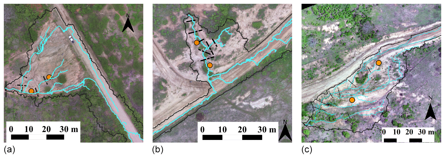
Figure 3Aerial photogrammetry of the gullies studied. Note that they are at the margin of the road, receiving the concentrated flow diverged from it. The continuous black line represents the catchment boundaries; the blue line represents the flow paths; the dashed black lines are the cross sections used in the validation of the model; and the orange dots are the soil sampling points: (a) gully 1, (b) gully 2 and (c) gully 3.
Table 1Coordinates of the three gullies used in this study (Datum: WGS84).

2.2 Topographic survey
The assessment of the gully data was achieved using an unmanned aerial vehicle (UAV), which is a technique that has also been applied in other regions (Stöcker et al., 2015; Wang et al., 2016; Agüera-Vega et al., 2017). A UAV equipped with a 16 MP camera (4000 pixels × 4000 pixels) and a 94 % field of view was used. The flight was at an altitude of 50 m with a frontal overlap of 80 % and a lateral overlap of 60 %. For the geo-reference of the mosaic, five ground control points were deployed that were evenly distributed in each area, both at high and low elevation. The coordinates were collected using a stationary Global Navigation Satellite System (GNSS) with real-time kinematic (RTK) positioning (L1/L2) with centimetre-level accuracy.
The digital surface model was produced using the structure from motion technique. This process consists of a 3D reconstruction of the surface derived from images and the generation of a dense cloud of 3D points based on the matching pixels of different pictures and ground control points (GPCs); the processing result is a model as accurate as that obtained by laser surveys (e.g. light detection and ranging – lidar), but it is cheaper and less time-consuming (Stöcker et al., 2015; Agüera-Vega et al., 2017). The ground sample distance (pixel size) obtained is 4–5 cm, and the digital models have high precision, with a vertical position error of 1 cm and a horizontal error of 0.6 cm. The vegetation, although sparse, was an obstacle to increasing the quality of the survey. However, as the focus of this study was the gully cross-section geometry, interference from vegetation was acceptably low.
2.3 Soil data
Due to the scale of this experiment and the homogeneity of the soil–vegetation components (Güntner and Bronstert, 2004), we divided the areas into two sets based on grain-size distribution, organic matter and bulk density. Gully 1 (G1) has specific features and represents the first soil type (S1), whereas gullies G2 and G3, which are close to each other, represent the second soil type (S2).
At the gully sites, soil surveys were carried out to assess the properties and parameters required to implement the model; undisturbed soil samples were collected (see Fig. 3) at depths of 0.10 m, 0.30 m and 0.50 m (two sites, three depths and three samples per depth, totalling 18 samples collected). At the depth of 0.50 m, a well-defined horizon C, rich in rocks and soil under formation, was identified. The maximum depth of the non-erodible layer ranged from 60 to 75 cm in all gullies. We performed grain-size distribution, sedimentation, organic matter, bulk density and particle density analysis.
The soils at the gully sites are loamy with a clay content ranging from 6 % to 37 %. The particle density is 2580 kg m−3. The soils are Luvisols and have a typical profile, with the top layer being relatively poor in clay compared with the layers below and with the regular occurrence of gravel at the surface. Furthermore, Luvisols are rich in active clay, which makes them prone to crack and macropore formation when dry (dos Santos et al., 2016); this is a process that has also been documented in soils with similar texture in a semiarid area in Spain (van Schaik et al., 2014). Rill erodibility values (Kr) and critical shear stress (τc) for the soils were obtained using Eqs. (1) and (2) (Alberts et al., 1995) and are also presented in Table 2.
where “%VFS” is the percentage of very fine sand, “%C” is the percentage of clay and “%OM” is the percentage of organic matter.
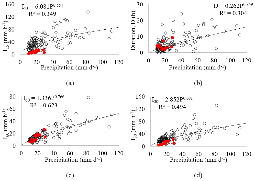
Figure 4Correlation between daily precipitation and sub-daily variables at the Aiuaba experimental basin (Figueiredo et al., 2016). (a) Daily precipitation versus event duration (D); (b) daily precipitation versus 60 min maximum intensity (I60); (c) daily precipitation versus 30 min maximum intensity (I30); and (d) daily precipitation versus 15 min maximum intensity (I15). The white circles indicate data obtained in Aiuaba from 2005 to 2014. The red dots indicate precipitation measured in the Madalena representative basin (MRB) from January to July 2019 (rainy season).
2.4 Rainfall data
Daily rainfall data for the location spanning the entire period were provided by the Foundation of Meteorology and Water Resources of Ceará (Funceme). We used five rain gauge stations in the region, covering the period from 1958 to 2015. The annual rainfall in the area averages 613 mm (Fig. S1 in the Supplement) with a coefficient of variation of 43 %, which are typical values for the Brazilian semiarid region (de Araújo and Piedra, 2009). The double-mass method was employed to check data consistency (Fig. S2). The gaps in the measurements (January 1958 and September 1960) were filled by the nearest gauging station.
The modelling of the gullies is based on peak discharge, which demands sub-daily rainfall data, but only daily precipitation was available inside the study basin covering the whole experiment period. To proceed with the modelling, correlation curves relating total daily precipitation and rainfall intensity were used. In order to define the best intensity to be used in the modelling, four were tested (Fig. 4) as input for the model: the average (Iav), the 60 min maximum (I60), the 30 min maximum (I30) and the 15 min maximum (I15).
To build such curves, we used data from the Aiuaba experimental basin (AEB). This basin has been monitored since 2005 (Figueiredo et al., 2016) and has detailed hydrographs, with 5 min temporal resolution. This experimental basin is located 190 km south of the MRB and both basins are climatically homogeneous (Mendes, 2010). In addition, Fig. 4 shows the rainfall data for the MRB collected during the rainy season in 2019 (January to July). We can observe that the data show similar behaviour but are constantly in the lower area of the plot. It is relevant to note that it was dry in the MRB in 2019 (total annual precipitation of 402 mm, which is over 30 % lower than the average) and such behaviour was expected.
To obtain discharge values from intensity, we used the soil conservation service curve number (SCS-CN) method (Chow, 1959). For the models, the main rainfall-related variables are the event peak discharge and its respective duration. Because the gully catchment areas were small, their respective concentration time was negligible compared with the intense-rainfall duration in the region (Figueiredo et al., 2016), yielding a uniform pattern of peak discharge.
Table 2Grain-size distribution, organic matter for both soils (S1 for the gully 1, and S2 for the gullies 2 and 3) at three depths (10, 30 and 50 cm) and the respective texture classification (USDA) as well as the estimated (in italic) rill erodibility (Kr) and critical shear stress (τc) of the site soils obtained using Eqs. (1) and (2).
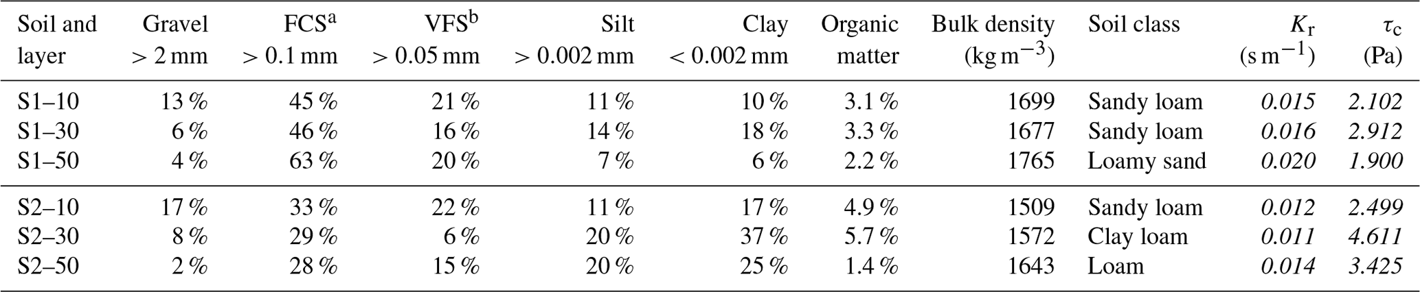
a Fine to coarse sand. b Very fine sand.
2.5 Gully modelling
To model small permanent gullies, we propose two models based on classical formulations from Foster and Lane (1983) and Sidorchuk (1999). The Foster and Lane model (FLM) is one of the most commonly used models of gully erosion and is based on net shear stress and transport capacity. The FLM assumes a rectangular cross section and was originally designed for single rainfall ephemeral gully modelling. The Sidorchuk model (SM) considers the mass balance of sediments, shear stress (in terms of critical velocity), soil cohesion and the Manning equation to estimate the cross-section geometry and channel slope. It also uses empirical equations based on field measurement to estimate the flow depth and width. This model pays special attention to the processes involving gully wall transformation. A description of both models is available in the literature and in the Supplement of this paper.
The proposed models are the adapted Foster and Lane model (FLM-λ) and the coupled Foster and Lane–Sidorchuk model (FL-SM). The key difference between the two proposed models is the amount of data required to use each one. The models are presented below.
2.5.1 Adapted Foster and Lane model (FLM-λ)
The Foster and Lane model (FLM), as proposed by its authors, considers a single source of erosion: the soil detached from the channels bed and walls due to shear stress. Field observation and the literature (Blong and Veness, 1982), however, show that wall instability and failure can represent a significant source of sediment. To estimate the effect of wall erosion at the study site, we proposed an empirical parameter (λ – Eq. 3) to correct the effect of lateral flow and wall erosion. This multiplicative parameter was calibrated and validated as a function of the catchment shape based on two coefficients: the Gravelius coefficient (KG – Eq. 4) and the Form coefficient (KF – Eq. 5). Both coefficients describe the geometry of the catchment area and can be interpreted as how compact the distribution of area is. Commonly linked to how flood prone an area is, these parameters also relate to the transversal distance of the catchment area, which influences the amount of lateral inflow into the mainstream.
In Eq. (3), the terms Ao and Am are the respective observed and measured cross-section area, and in Eqs. (4) and (5), CP, CA and CL stand for the catchment perimeter, area and length respectively.
The plots of λ versus both parameters are presented in Fig. 5. Two equations, λ(KG) and λ(KF) (see Fig. 5), were calibrated using data from 14 randomly selected sections from the 21 assessed by the DEM. The remaining data were used to validate the equations. The FLM-λ model consists of processing the FLM as originally proposed and, afterwards, multiplying the output area by the λ correction parameter. As λ≥1.0, the multiplication simulates the effect of wall erosion.
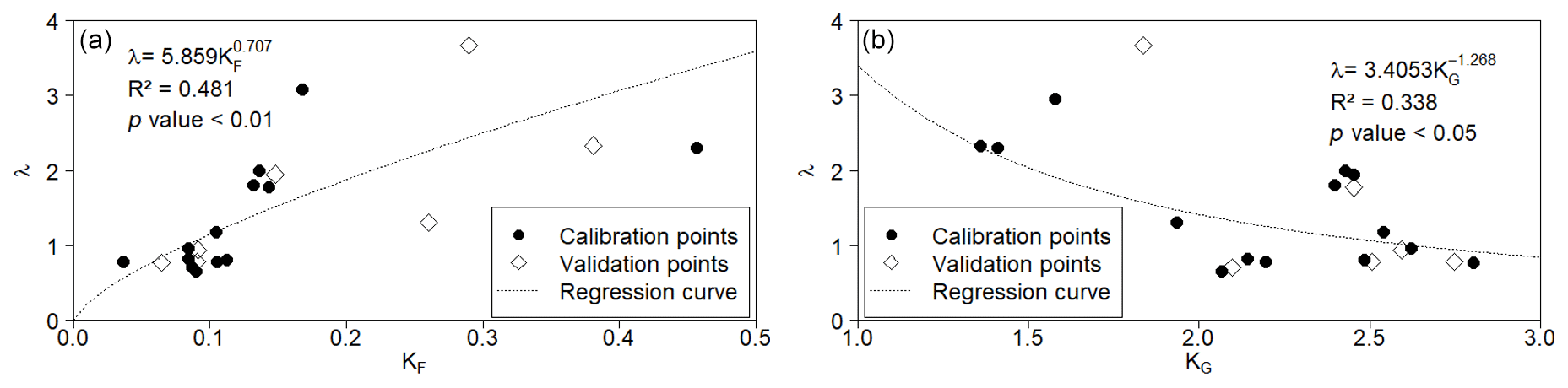
Figure 5Correlations between the ratio (λ = Ao∕Am) and (a) the Gravelius coefficient (KG) and (b) the form factor (KF) for 21 monitored cross sections at the Madalena representative basin (MRB). Black dots refer to calibration cross sections, and white diamonds refer to validation cross sections. The R2 values indicated in the plots are for the calibration. The validation R2 values were 0.10 for KG and 0.54 for KF.
The coefficient (KF) yielded a positive Nash–Sutcliffe efficiency value and a smaller RMSE (0.17 and 0.67 respectively) which did not occur with the Gravelius coefficient (−2.43 and 0.84 respectively). In the revised model, hereafter referred to as FLM-λ, the FLM area output is multiplied by the calibrated parameter λ (Eq. 6), yielding the eroded area. Applying this factor caused a significant improvement in model efficiency, with the NSE increasing from 0.557 to 0.757. The incremental area produced by the multiplication of λ is assumed to increase the width of the upper half of the cross section, while the bottom width and the orthogonality of the walls remain unchanged.
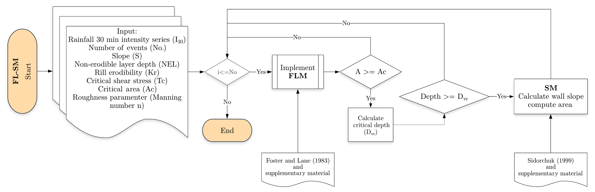
2.5.2 The coupled Foster and Lane–Sidorchuk model (FL-SM)
The previous model was produced due to the necessity of considering wall failure as a sediment source and was used an empirical approach. Another method, using a physically based concept, is to include the specific routine of the Sidorchuk model that tackles wall failure in the Foster and Lane model. This can be achieved by simply including a test after each event that checks if the depth of the channel causes wall instability given the current angle of the bank.
By analysing the data, however, we identified that for small cross sections, even after the critical depth had been reached, the section remained rectangular. This implies an additional threshold mechanism related to the geometry of the channel and/or catchment. Therefore, the FL-SM requires the determination of a threshold value for the implementation of the wall erosion equations. This threshold controls when the wall erosion becomes significant for the total amount of eroded soil. In the model, it represents the limit above which Sidorchuk (1999) equations are used. It also represents the scale when the channel bed erosion alone, described by the Foster and Lane (1983) equations, begins to consistently underestimate the measured area. In this study, we used the Foster and Lane (1983) model to identify the threshold where both processes (channel bed and wall erosion) switch relevance.
A flow chart of the FL-SM model is presented in Fig. 6. The core of the model is the Foster and Lane (1983) model, processed for every runoff event. When the cross section reaches the threshold condition and satisfies the criteria for wall failure as described in Sidorchuk (1999), a new step is included that calculates wall transformation.
2.6 Model fitness evaluators
To assess the goodness of fit, the Nash–Sutcliffe efficiency coefficient (NSE), the root-mean-squared error (RMSE) and the percent bias (PBIAS) were used (see Moriasi et al., 2007). Additionally, the methodology proposed by Ritter and Muñoz-Carpena (2013) asserts statistical significance to the evaluators. The proposed model is based on Monte Carlo sample techniques to reduce subjectivity when assessing the goodness of fit of models.
In Eqs. (7)–(9), Xo, i is an observation, Xm, i a modelled value, n is the total of observations or simulations, and is the average of the observed values.
3.1 Gully modelling
From the three gullies measured, 21 cross sections with different dimensions were selected and used to validate and compare the models' quality. Fig. 7 presents the scatter of modelled and measured data for the models implemented. The FL-SM presented a Nash–Sutcliffe efficiency coefficient of 0.846 when using a threshold for the area of the cross section of 2.2 m2. Some output examples for the sections above the threshold are presented in Fig. 8.
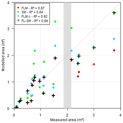
Figure 7Performance of the coupled model (FL-SM), the Foster and Lane (1983) model (FLM and FLM-λ) and the Sidorchuk (1999) model (SM). p value <0.001 for all sets. The grey bar indicates the identified threshold area where there is a change and the SM becomes consistently better than the FLM.
In terms of geometry, sections modelled with the original Foster and Lane (1983) model present output cross sections, similar to Fig. 8a, b and c, with a rectangular-like shape. When the parameter λ is introduced (FLM-λ), the output cross sections are modelled with piled rectangles, as in Fig. 8d, e and f. Using the FL-SM, when the area surpasses the threshold value, sections mainly have trapezoidal geometry, as illustrated in Fig. 8g, h and i. It is important to highlight that the model can produce triangular geometry, but this was observed in this study.
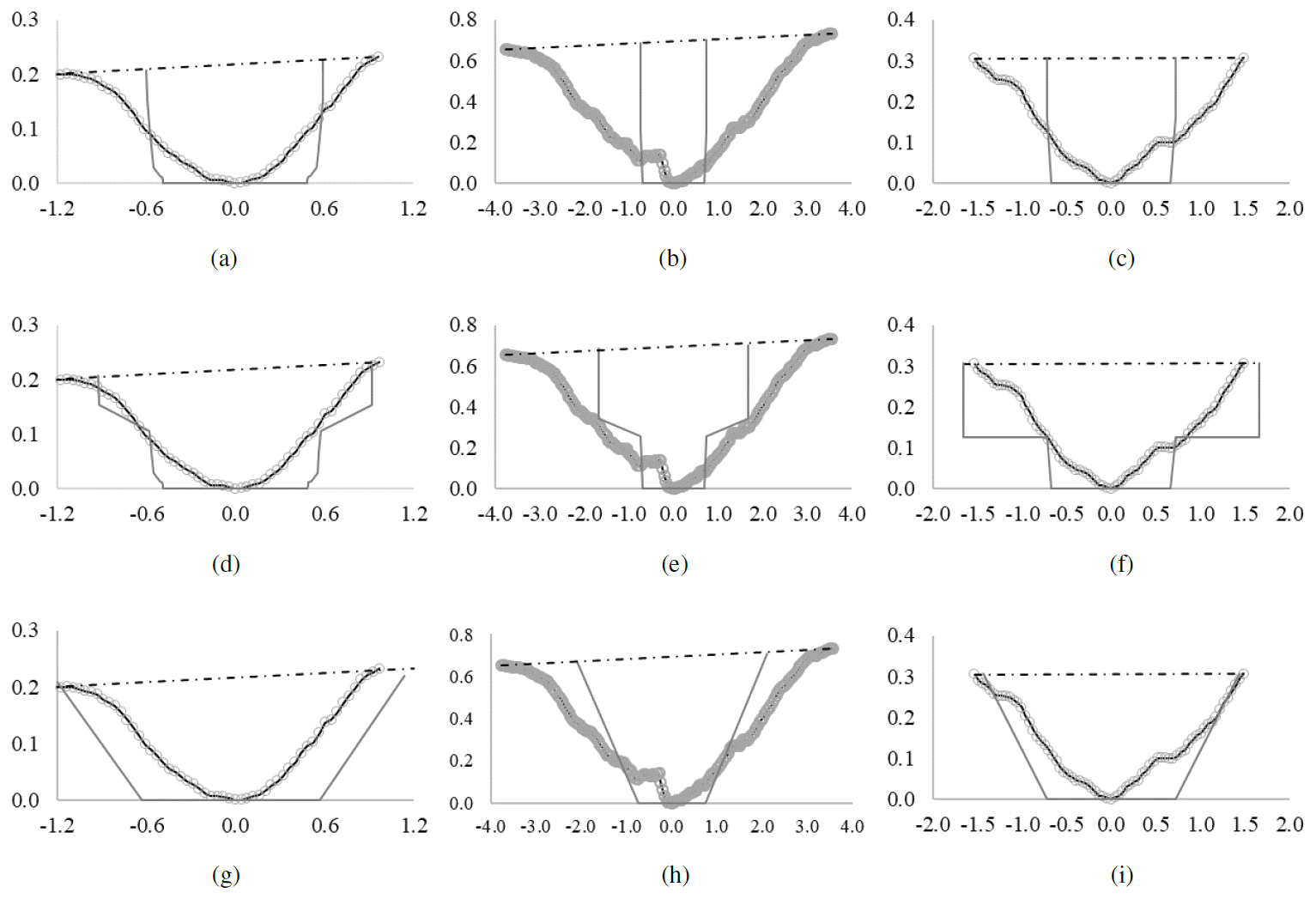
Figure 8Some examples of the gully cross sections measured (black line with circles) and the modelled (dark grey line) geometry. Panels (a), (b) and (c) show the output of the Foster and Lane (1983) model; panels (d), (e) and (f) show the output of the adapted Foster and Lane model with the parameter λ; and panels (g), (h) and (i) show the result from the Sidorchuk (1999) model (SM). Distances are give in metres. The section in (a), (d) and (g) is obtained from gully 1; the section in (b), (e) and (h) is from gully 2; and the section from (c), (f) and (i) is from gully 3.
3.1.1 Threshold analysis
The interpretation of the threshold for the implementation of the wall erosion routine can be based on (a) the cross-section area or (b) the catchment geometry, as illustrated in Fig. 9. The first approach considers a critical area that, once reached, marks when the wall erosion is truly significant with respect to the other processes. In this study, this threshold identified was at an area of 2.2 m2. After this level is reached, the model calculates the effect of sidewall erosion and gains the critical final area for the section analysed. The presence of a threshold for applying the sidewall erosion routine indicates a change in the relevance of processes at a given scale. Although the threshold is addressed as an area, this is only a consequence of more complex interactions among discharge, flow erosivity, cohesion and gravitational forces.
The second interpretation is related to the catchment geometry, as the approach given to the parameter λ is also related to the KF. From the distribution of the cross sections, we can observe sections that are better modelled by SM – even below the threshold. By analysing the values of the form coefficient (KF) of each set (Fig. 9b), we observed that set 1 has a KF of 0.08 (±0.02) and set 2 has a KF 0.22 (±0.12). Higher KF values indicate a more compact catchment with more lateral flux into the channel, which, in turn, produces more erosion in the soil. By sorting the model results from FLM and SM based on the form coefficient, using the threshold of KF=0.15, we obtained an NSE of 0.79.
Given the efficiencies obtained in this study, we adopted a threshold based on the cross-section area. However, the use of a catchment-based threshold should not be discarded and could be promising due to the fact that there are reports in the literature of a relation between lateral flow and gully erosion (Blong and Veness, 1982).
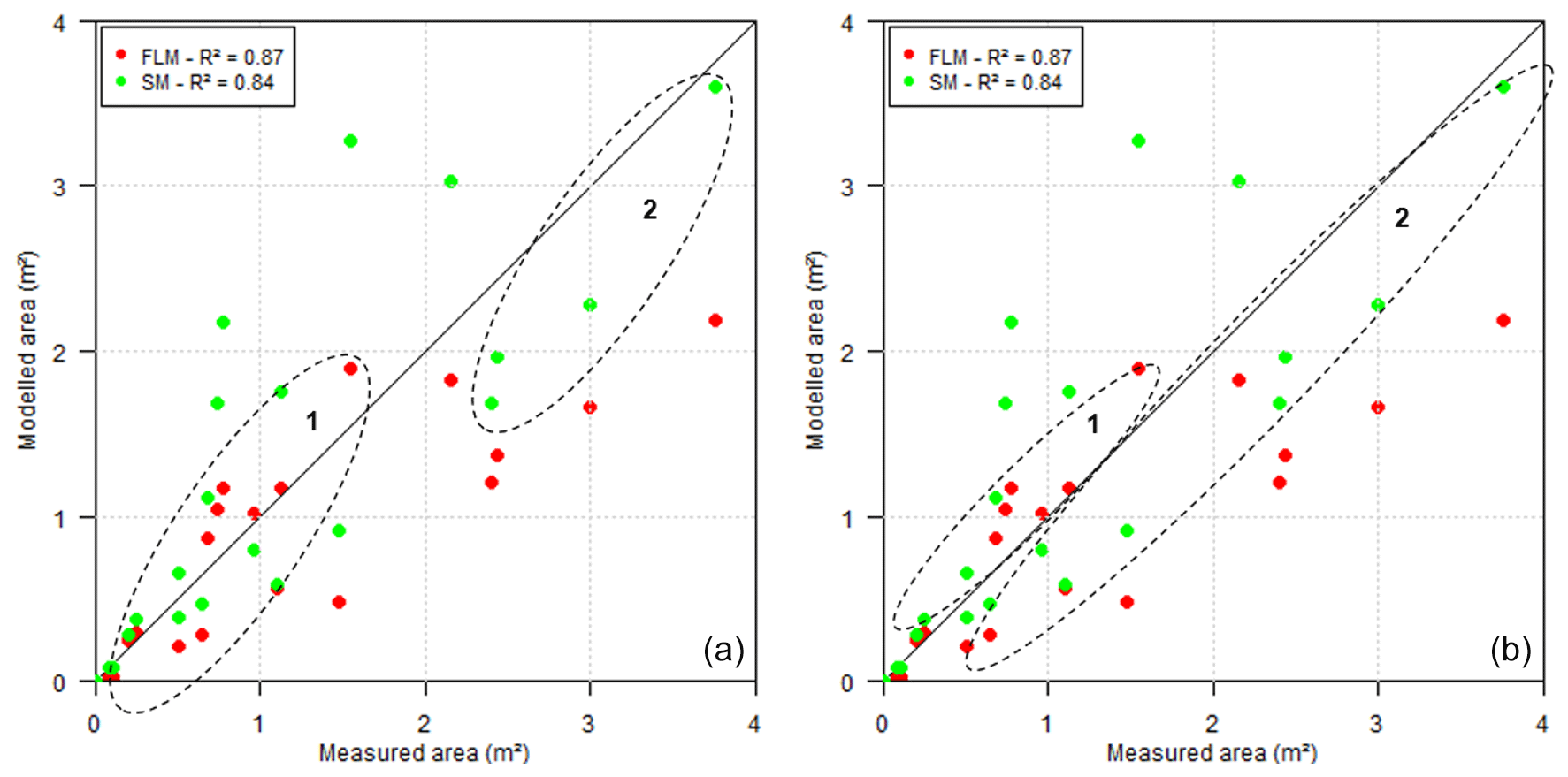
Figure 9Thresholds for wall erosion (a) based on the cross-section area and (b) based on the catchment geometry and KF. In both plots, set 1 indicates the domain of bed erosion and the Foster and Lane (1983) equations, and set 2 indicates the domain of wall erosion and the Sidorchuk (1999) equations. p value <0.001.
3.1.2 Rainfall intensity
From the three gullies, 21 cross sections with no interference from bushes or trees were selected from the digital elevation model. The FLM was tested for the 60, 30, 15 min and average intensities – FLM(I60), FLM(I30), FLM(I15) and FLM(Iav) respectively. The best response was shown when using the 30 min intensity, FLM(I30) (NSE =0.557). Figure 10 presents the plot of the model outputs for the cross-section area compared with the measured data. Moreover, the Foster and Lane (1983) model did not show good responses to the cross-section geometry, regardless of the intensity tested. This may indicate a flaw in the model concerning the sideward erosive process.
The FLM considers rectangular-shaped cross sections, but the field survey showed that the sections were actually trapezoidal or triangular (Fig. 8). Among the factors that can shape gully walls, some examples include seepage, the angle of internal friction and the slope angle itself (Sidorchuk, 1999; Bingner et al., 2016). Besides this, gully walls can be shaped by lateral discharge (Blong and Veness, 1982) which depends directly on the morphology of the cross section's catchment area. Figure 10 also shows the tendency of the model to underestimate the cross-section area, which implies that the model does not consider all of the relevant erosive processes. The sidewall erosion has proven to be a relevant source material, often representing over 50 % of the eroded mass (Crouch, 1987); however, the FLM only assumes the vertical sidewall morphology. Therefore, in this study, we adopted the 30 min intensity as the standard intensity and duration to assess peak discharge.

Figure 10Results of the FLM for a cross-section area using different intensities – Iav (average), I60 (60 min), I30 (30 min) and I15 (15 min) – to generate the peak discharge.
3.2 Model evaluators
The coupled model, FL-SM, presented the highest performance of goodness of fit evaluators (Fig. 11). The model yielded a PBIAS value below 10 %, which is very good. The coupled model's RMSE was also low (0.397), whereas the NSE reached a value of 0.846, which is classified as good (Ritter and Muñoz-Carpena, 2013) or very good (Moriasi et al., 2007).
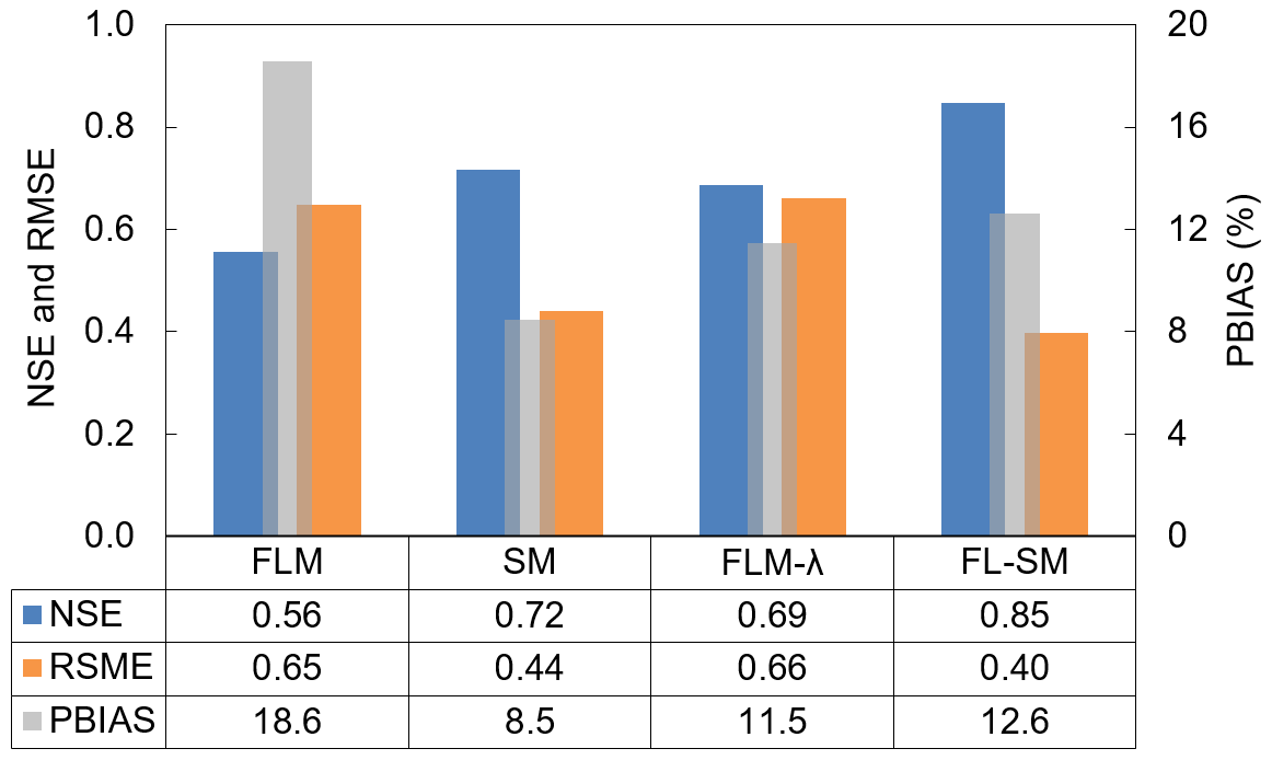
Figure 11Model evaluators: NSE, RMSE and PBIAS. The bar plot shows the performance of all tested models; the PBIAS values are given in percent.
Figure 11 shows the evolution of NSE values in more detail to allow for conclusions be drawn. The Foster and Lane (1983) model with the λ parameter (FLM-λ) was calibrated with 14 cross sections from the 21 and performed as well as the Sidorchuk (1999) model (SM), which considers the sidewall effect. For the coupled model, there is no efficiency gain when applying the calibrated parameter (λ) to sections below the threshold which indicates that the lateral inflow is only relevant for larger sections. Figure 12 presents a Taylor diagram to compare the four models. In this diagram, the closer a model is to the reference (measured data), the better. The FL-SM presented the highest correlation and the lowest RMSE value.
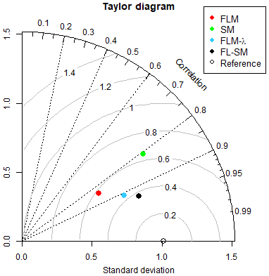
Figure 12Taylor diagram comparing model performance. The azimuthal distance gives the correlation (R, Pearson). The distance to the origin is proportional to the standard deviation of the model values, and the distance to the reference (measured data) is proportional to the RMSE.
We also used the strategy of Ritter and Muñoz-Carpena (2013), the FITEVAL. The concept behind this strategy is a Monte Carlo approach to the Nash–Sutcliffe efficiency computation. Using repeated resampling from the data set, their method delivers a probability density function to the NSE. This allows for an uncertainty analysis for the evaluator. The FL-SM presented an NSE ∈ [0.66; 0.95] for a p value of 0.05, which is classified as acceptable to very good. A conservative interpretation of this result implies considering the lowest values as the minimum state of information or as the value that contains (almost) no unproven hypothesis. As a consequence, and according to Ritter and Muñoz-Carpena (2013), the FL-SM can be classified as acceptable to very good. The detailed output of the FITEVAL analysis can be found in the Supplement (Fig. S6).
3.3 Gully growth modelling
Gully growth is commonly described as being a fast process in the first years that progressively slows down as it enlarges. In our model, the mechanism that produces this dynamic is known as “event piling”. For example, after a particularly intense event, it was observed that the channel was wide enough; therefore, the following less-intense events only produced shallow flow and low shear stress, resulting in less or no sediment compared with the previous event. Thus, further erosion only occurs due to a more intense event than the last erosive one.
Our model mimics this growth dynamic and the periods between extreme events. Such behaviour has been widely explored in the literature (Vanwalleghem et al., 2005; Poesen et al., 2006; Poesen, 2018) and is illustrated in Fig. 13. Using several data sets from previous studies, Vanwalleghem et al. (2005) found a strong correlation between GT (the percentage of the gully age over the total) and GV (the percentage of the gully volume over the total), given by the function expressed in Eq. (10). The parameters α and β were calibrated by Vanwalleghem et al. (2005) as 96.5 and -0.07 with a coefficient of determination (R2) equal to 0.99.
The parameters α (equal to 100) and β (equal to −0.22) obtained in our study differ from values in the literature. While the difference in α is due to a numerical formulation (GVtotal is equal to the measured volume), the parameter β brings us some insights. Its absolute value for our data set is 3 times larger than that calibrated by Vanwalleghem et al. (2005). A larger indicates a fast initial growth, possibly caused by the intensive rainfall regime of the region, with convective intense events and high erosivity (Medeiros and Araújo, 2014). These are different conditions from Belgium and Russia, where most studies that led to the Vanwalleghem et al. (2005) equation were carried out. Therefore, although gully growth behaviour is similar in different regions, local conditions such as climate and land use should be taken into account.
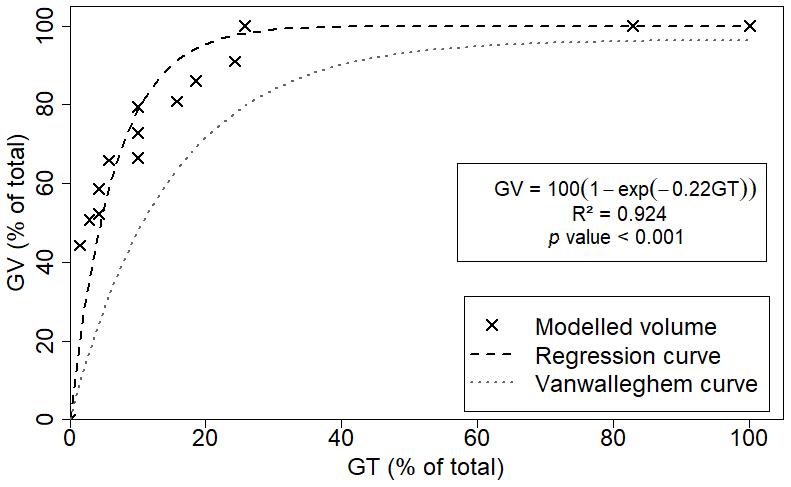
Figure 13The behaviour of the gully growth rate as proposed in the literature (Vanwalleghem et al., 2005; Poesen et al., 2006) and modelled (data from gully 1). GV is the gully volume (in percent) and GT the gully age (in percent).
3.4 Landscape development impacts on gully erosion
Gullies are scale-dependent phenomena and are frequently related to thresholds due to their initiation, which is based on catchment area and slope (Torri and Poesen, 2014; Poesen, 2018). Both characteristics are directly linked to shear stress and stream power when using physical gully models. Montgomery and Dietrich (1992) argue that changes in the landscape and the drainage system can lead to a larger occurrence of channelization and its impacts can be noticed more quickly. Torri and Poesen (2014) suggest a threshold for head development in gullies as conveyed in Eq. (11).
where S (m m−1) is the slope, CA (ha) is the catchment area, and k is a parameter for channel and gully initiation.
For croplands in tropical conditions, the proposed value of k is 0.042 (Torri and Poesen, 2014). For the areas in the present study, we have channel initiation for values less than half (k=0.020) of the above-mentioned k value, and systematically lower values than the field data of Vandaele et al. (1996) were also observed. These findings suggest the vulnerability of the region to gully formation. Considering that the three experimental sites were located next to a road, this disturbance triggered gully initiation, and other actions (such as deforestation and forest fire) may cause similar problems in the region. The roads have not only enlarged the total catchment area but have also increased its length. While relations between catchment length and area are well established () with values of b varying from 1.78 to 2.02 (Montgomery and Dietrich, 1992; Sassolas-Serrayet et al., 2018), the present experiments found a b value of 3.17. With a smoother surface and almost no meandering, road construction causes modifications that promote more energetic flows on the gully head. Road construction has also been identified as a potential factor for gully initiation in other areas of the Brazilian semiarid region, such as in the Salitre Catchment, where large gullies initiated after the construction of an unpaved rural road (da Silva and Rios, 2018).
4.1 Model limitations
The proposed models, especially the FL-SM, presented a significant improvement, reaching an efficiency of over 0.8. However, some reflections can be made to understand when the models fail as well as to understand where new advances can be pursued.
4.1.1 The Foster and Lane model (FLM)
The FLM requires a peak discharge duration input. Given the lack of such data in the region, our first step in this study was to identify the best peak and duration of rainfall values to be considered based on the rainfall intensity. Therefore, a relevant result from this work is the confirmation that the 30 min intensity is the value that provides the most information about gully erosion. Wischmeier and Smith (1978) proposed the product of the total storm energy and the 30 min intensity to “predict the long-time average soil loss in runoff”. The use of I30 for estimating event-related gully erosion was previously experimentally tested by Han et al. (2017). The authors monitored a gully in the Loess Plateau in China for 12 years, registering 115 erosive rainfall events. They concluded that the product of the 30 min intensity and total precipitation (P I30) was the key parameter to estimate total soil loss. Our results corroborate this.
Furthermore, by applying the I30 in this study in order to estimate peak discharge and duration, it is implied that all of the energy necessary to initiate and develop a gully channel comes from the most intense 30 min. Due to the limited number of gullies, it is not straightforward that the I30 would be the most representative index for any situation. Peak discharge and critical rainfall duration are often central variables in gully models (Foster and Lane, 1983; Hairsine and Rose, 1992; Sidorchuk, 1999; Gordon et al., 2007) and are related to erosion initiation parameters and thresholds, such as shear stress and stream power. This latter factor has frequently been reported in the literature as being more correlated with both laminar and linear erosion (Bennett and Wells, 2019). Figure 10a shows the performance of the intensities tested. Although the model using the 15 min intensity presented smaller PBIAS and RMSE values, the results indicated a large scatter around the average.
Finally, the Foster and Lane (1983) model also considers a fixed shear distribution, which is often unrealistic (Bonakdari et al., 2014) and has a fixed rectangular shape that, although frequently accurate for ephemeral gullies, does not agree with field data or the literature (Fig. 8; Starkel, 2011).
4.1.2 The Sidorchuk model (SM)
The SM produced good results in this study which were similar to those obtained by inserting a calibrated factor (λ) in FLM. It is important to note that the original model used empirical correlations to determine width (Sidorchuk, 1999; Nachtergaele et al., 2002) and these were obtained using data from the Yamal Basin. In the present study, we substituted this approximation for the width estimated by the FLM model, which permitted a more physical approach and increased the quality of the SM. The model was also capable of predicting the sidewall slope well.
The model, however, showed a trend of overestimating smaller cross sections (see Fig. 7), which was mainly due to section geometry. When applied, the bottom width of the channel is considered to be the final width obtained by FLM. In larger sections, this hypothesis holds once the discharge is large enough to carry all of the soil produced by sidewall erosion. In smaller sections, part of the soil is deposited and produces a V- or U-shaped cross section (Starkel, 2011).
4.1.3 Proposed models
The FLM was further improved by the addition of the calibrated parameter λ (FLM-λ). This parameter was included to predict the effect of lateral discharges over wall erosion. Due to the significant improvement produced by its insertion, it could be understood that the original FLM fails to tackle this source of material (Blong and Veness, 1982; Crouch, 1987).
The FL-SM considers two sediment sources: channel bed and sidewall. However, gullies are complex systems with many sources and interactions. Headcut, sidewall erosion due to raindrops, flow jets and piping were not considered in our modelling approach. Processes of infiltration, subsurface flow and transport capacity were also neglected and should be properly addressed in future work. Nevertheless, the FL-SM assumptions managed to mimic the field measurements well, which implies that, at least in this study, the neglected processes are of lower relevance or were considered indirectly. For instance, sidewall erosion by raindrops can be considered insignificant over the wall failure process considered by Sidorchuk (1999). In addition, it is important to note that, by selecting the 30 min intensity, a less intense interval might be overlooked that also produces erosive discharge and can, therefore, explain the remaining processes.
One advantage of the FLM-λ over the FL-SM is that the former requires less data than the latter. The Sidorchuk model and, consequently, the FL-SM require extra fieldwork and laboratory analysis to assess root mass and plasticity index.
Despite the good results obtained from the modelling, the use of stochastic approaches and the introduction of other sources of sediment (Sidorchuk, 2005) should improve the performance of the model. This is also relevant for generalization and modelling of classical gullies. In the same way, the introduction of processes such as armouring and energy losses, as proposed by Hairsine and Rose (1992), can be interpreted as probabilistic terms.
Compared with the other models, either physical or empirical (Hairsine and Rose, 1992; Woodward, 1999; Wells et al., 2013; Dabney et al., 2015), our proposed model (FL-SM) requires a similar amount or less data, little calibration (one parameter – the threshold) and is more versatile. Most models fail to account for multiple rainfall events (Foster and Lane, 1983; Woodward, 1999; Nachtergaele et al., 2002) and do not consider multiple sources of sediment (Foster and Lane, 1983; Hairsine and Rose, 1992; Dabney et al., 2015). The FL-SM model presented a better performance index (R2=0.94) than empirical models, e.g. R2 values of 0.55 and 0.12 for Woodward (1999) and Wells et al. (2013) respectively, and physical models, e.g. R2 values of 0.87 and 0.84 for Foster and Lane (1983) and Sidorchuk (1999) respectively. This enhancement of the performance can be accounted for by the more detailed modelling, which considers wall failure and non-rectangular cross sections.
4.2 Data limitations
4.2.1 Topographic data
In terms of accuracy and agility, a topographic survey with a UAV permits the measurement of sites within a few minutes. Conventional measurements, such as those with a total station or profilometer, are more time-consuming and do not grant better resolutions. The UAV accuracy, however, can be enhanced by performing flights at lower heights and with more GCPs (Agüera-Vega et al., 2017; James et al., 2017), as well as by using high-end equipment, such as more robust UAVs and stabilizers. Total stations can also be used to improve the accuracy of GCPs (Mesas-Carrascosa et al., 2016). Given the scale of this study and the presented results of the models, the 4 cm pixel represents a good resolution, as it combines good precision at an affordable computational costs (Wang et al., 2016). The solution of a UAV-based volume assessment is a good option for monitoring gully evolution (Stöcker et al., 2015), as it allows frequent surveys, e.g. after every intense rainfall event.
However, trees and bushes obscure topographic measurements if they are too close to the gully channel and/or too dense in the catchment. Thus, UAV monitoring is more reliable for gully sites in non-vegetated or sparsely vegetated areas and meadows, which concurs with the conditions of this study, except for gully 3 (G3) where it was impossible to accurately measure the total erosion volume due to relatively dense vegetation. It was, however, possible to select a large enough number of sections (eight) at G3 to assess the total erosion volume.
The topographic survey showed that all gullies had a significant portion of their watersheds occupied by the road, indicating a modification of the drainage system and a change in the catchment boundaries – both causes of gully initiation foreseen by Ireland et al. (1939) – due to road construction, which promoted intense runoff and triggered gullies. Impacts of road construction on gully formation were also observed in Ethiopia (Nyssen et al., 2002) and in the USA (Katz et al., 2014). Considering these previous records in the literature and the information collected from locals, the modelling considered 1958 as the start of gully erosion, coinciding with road construction.
4.3 Soil data
Although the three gullies studied are located in the same mesoscale basin, the Caatinga biome is known for its soil variability (Güntner and Bronstert, 2004) and soil properties do differ among the gullies. However, only small changes in texture were observed at different depths, allowing an analysis based on average properties. Nevertheless, for deeper and/or more variable soils, the discretization of soil properties and, therefore, parameters such as rill erodibility (Kr) and critical shear stress (τc) can easily be taken into account. The good performance of the final model (FL-SM) also indicates that the Water Erosion Prediction Project (WEPP) equations for critical shear stress and rill erodibility (Eqs. 1 and 2) can be used for the soils of the region. These equations were obtained via regression curves from data collected on 34 plot areas in the USA with a wide range of textures, slopes, land uses and land covers. The areas from the WEPP model possess different geological and climatic conditions from the soils in the Brazilian semiarid region; this is why local studies should be carried out, given that empirical equations frequently have a strong local character (Ghorbani-Dashtaki et al., 2016; Dionizio and Costa, 2019).
4.4 Rainfall data
This study shows that sub-daily information of rainfall is of crucial importance for gully modelling. In this study, we used correlation curves based on long-term time series of a similar catchment in the region. However, such analysis might introduce an averaged and monotonic behaviour for the intensities, as presented in Fig. 4, and is, therefore, unrealistic. Stochastic models should be tested to estimate sub-daily information from daily rainfall. The estimation of discharge from rainfall can also be improved by considering water content in the soil and modelling its evolution over the studied period using water balance models.
In this study, we proposed and tested two new gully models based on two previous models (Foster and Lane, 1983, and Sidorchuk, 1999). We also investigated which rainfall intensity is best suited for gully modelling when sub-daily rainfall data are not available, finding the 30 min intensity (I30) to be the most appropriate.
The models present a significant improvement when compared with other models from the literature. While the FLM-λ requires less calibration, the FL-SM presented better results, not only in terms of total gross erosion but also in terms of gully growth dynamic. Through modelling and fieldwork, it was also possible to identify the effects of landscape change and climatic conditions on gully development in the region. Gully erosion is an erosion related to many processes and is scale dependent. The attempt to propose a generalist model for gullies should also consider these different scales and the mechanisms involved in different stages of the gully development. Catchment shape and lateral flow have a central role in gully erosion, and their influence should be further investigated. Infrastructure construction, like roads, changes the conditions for gully initiation and was the trigger for the gullies in this study.
Nonetheless, further efforts are required to fully model gully erosion, such as the inclusion of multiple other sources such as headcut, pipping, channel shear stress and flow jets. Also, stochastic modelling should be implemented in order to tackle the inherent uncertainties of many sediment sources and the lack of data.
The code and data are available at https://doi.org/10.5281/zenodo.3485064 (Alencar et al., 2019).
The supplement related to this article is available online at: https://doi.org/10.5194/hess-24-4239-2020-supplement.
PHLA carried out fieldwork, programming and laboratory analysis and prepared the text with contributions from all co-authors. AdST undertook image acquisition and processing. JCdA supervised the work and was instrumental in its conception.
The authors declare that they have no conflict of interest.
This study was partly financed by the Coordenação de Aperfeiçoamento de Pessoal de Nível Superior – Brasil (CAPES; finance code 001, CAPES/Print grant no 88881.311770/2018-01) and by Edital Universal (CNPq grant no. 407999/2016-7. Pedro Alencar is funded by the DAAD (award no. 91693642). The authors are grateful to Eva Paton from the TU Berlin for support and advice.
This research has been supported by the Coordenação de Aperfeiçoamento de Pessoal de Nível Superior – Brasil (CAPES; finance code 001, CAPES/Print grant no. 88881.311770/2018-01), the Edital Universal (CNPq grant no. 407999/2016-7) and the DAAD (award no. 91693642).
This open-access publication was funded
by Technische Universität Berlin.
This paper was edited by Roberto Greco and reviewed by Xuanmei Fan and one anonymous referee.
Agüera-Vega, F., Carvajal-Ramírez, F., and Martínez-Carricondo, P.: Assessment of photogrammetric mapping accuracy based on variation ground control points number using unmanned aerial vehicle, Measurement, 98, 221–227, 2017. a, b, c
Alberts, E. E., Nearing, M. A., Weltz, M. A., Risse, L. M., Pierson, F. B., Zhang, X. C., Laflen, J. M., and Simanton, J. R.: Soil Component, Tech. Rep. July, USDA, West Lafayette, Indiana, 1995. a
Alencar, P. H. L., de Araújo, J. C., and dos Santos Teixeira, A.: PedroAlencarTUB/GullyModel-FLSM: Initial version (Version v1.0.0), Zenodo, https://doi.org/10.5281/zenodo.3485064, 2019. a
Arabameri, A., Cerda, A., and Tiefenbacher, J. P.: Spatial Pattern Analysis and Prediction of Gully Erosion Using Novel Hybrid Model of Entropy-Weight of Evidence, Water, 11, 1129, https://doi.org/10.3390/w11061129, 2019. a
Azareh, A., Rahmati, O., Rafiei-Sardooi, E., Sankey, J. B., Lee, S., Shahabi, H., and Ahmad, B. B.: Modelling gully-erosion susceptibility in a semi-arid region, Iran: Investigation of applicability of certainty factor and maximum entropy models, Sci. Total Environ., 655, 684–696, https://doi.org/10.1016/j.scitotenv.2018.11.235, 2019. a
Bennett, S. J. and Wells, R. R.: Gully erosion processes, disciplinary fragmentation, and technological innovation, Earth Surf. Proc. Land., 44, 46–53, https://doi.org/10.1002/esp.4522, 2019. a, b
Bernard, J., Lemunyon, J., Merkel, B., Theurer, F., Widman, N., Bingner, R., Dabney, S., Langendoen, E., Wells, R., and Wilson, G.: Ephemeral Gully Erosion – A National Resource Concern., NSL Technical Research Report No. 69, U.S. Department of Agriculture, Washington, D.C., 67 pp., 2010. a, b
Bingner, R. L., Wells, R. R., Momm, H. G., Rigby, J. R., and Theurer, F. D.: Ephemeral gully channel width and erosion simulation technology, Nat. Hazards, 80, 1949–1966, https://doi.org/10.1007/s11069-015-2053-7, 2016. a
Blong, R. J. and Veness, J. A.: The Role of Sidewall Processes in Gully Development, Earth Surf. Proc. Land., 7, 381–385, 1982. a, b, c, d
Bonakdari, H., Sheikh, Z., and Tooshmalani, M.: Comparison between Shannon and Tsallis entropies for prediction of shear stress distribution in open channels, Stoch. Env. Risk. A, 29, 1–11, https://doi.org/10.1007/s00477-014-0959-3, 2014. a
Borrelli, P., Robinson, D. A., Fleischer, L. R., Lugato, E., Ballabio, C., Alewell, C., Meusburger, K., Modugno, S., Schütt, B., Ferro, V., Bagarello, V., Oost, K. V., Montanarella, L., and Panagos, P.: An assessment of the global impact of 21st century land use change on soil erosion, Nat. Commun., 8, 2003, https://doi.org/10.1038/s41467-017-02142-7, 2017. a
Castillo, C. and Gómez, J. A.: A century of gully erosion research: Urgency, complexity and study approaches, Earth-Sci. Rev., 160, 300–319, https://doi.org/10.1016/j.earscirev.2016.07.009, 2016. a
Chow, V. T.: Open-channel hydraulics, in: Open-channel hydraulics, McGraw-Hill, West Caldwell, NJ, 1959. a
Coelho, C., Heim, B., Foerster, S., Brosinsky, A., and de Araújo, J. C.: In situ and satellite observation of CDOM and chlorophyll-a dynamics in small water surface reservoirs in the brazilian semiarid region, Water (Switzerland), 9, 913, https://doi.org/10.3390/w9120913, 2017. a, b, c, d
Conoscenti, C. and Rotigliano, E.: Predicting gully occurrence at watershed scale: Comparing topographic indices and multivariate statistical models, Geomorphology, 359, 107123, https://doi.org/10.1016/j.geomorph.2020.107123, 2020. a, b
Crouch, R. J.: The relationship of gully sidewall shape to sediment production, Aust. J. Soil. Res., 25, 531–539, 1987. a, b
Dabney, S. M., Vieira, D. A. N., Yoder, D. C., Langendoen, E. J., Wells, R. R., and Ursic, M. E.: Spatially Distributed Sheet, Rill, and Ephemeral Gully Erosion, J. Hydrol. Eng., 20, C4014009, https://doi.org/10.1061/(ASCE)HE.1943-5584.0001120, 2015. a, b, c
da Silva, A. J. P. and Rios, M. L.: Alerta de desertificação no médio curso do Rio Salitre, afluente do Rio São Francisco, Tech. rep., IFBA, Senhor do Bonfim, Bahia, 2018. a
de Araújo, J. C. and Piedra, J. I. G.: Comparative hydrology: analysis of a semiarid and a humid tropical watershed, Hydrol. Process., 23, 1169–1178, https://doi.org/10.1002/hyp.7232, 2009. a
de Araújo, J. C., Güntner, A., and Bronstert, A.: Loss of reservoir volume by sediment deposition and its impact on water availability in semiarid Brazil/Perte de volume de stockage en réservoirs par sédimentation et impact sur la disponibilité en eau au Brésil semi-aride Loss of reservoir volume by se, Hydrolog. Sci. J., 51, 157–170, https://doi.org/10.1623/hysj.51.1.157, 2006. a, b
Dionizio, E. A. and Costa, M. H.: Influence of Land Use and Land Cover on Hydraulic and Physical Soil Properties at the Cerrado Agricultural Frontier, Agriculture, 9, 24, https://doi.org/10.3390/agriculture9010024, 2019. a
dos Santos, J. C. N., de Andrade, E. M., Guerreiro, M. J. S., Medeiros, P. H. A., de Queiroz Palácio, H. A., and de Araújo Neto, J. R.: Effect of dry spells and soil cracking on runoff generation in a semiarid micro watershed under land use change, J. Hydrol., 541, 1–10, https://doi.org/10.1016/j.jhydrol.2016.08.016, 2016. a
Figueiredo, J. V., Araújo, J. C., Medeiros, P. H. A., and Costa, A. C.: Runoff initiation in a preserved semiarid Caatinga small watershed, Northeastern Brazil, Hydrol. Process., 30, 2390–2400, https://doi.org/10.1002/hyp.10801, 2016. a, b, c, d
Foster, G. R. and Lane, L. J.: Erosion by concentrated flow in farm fields, in: D. B. Simons Symposium on Erosion and Sedimentation, Colorado State University, Fort Collins, CO, p. 21, 1983. a, b, c, d, e, f, g, h, i, j, k, l, m, n, o, p, q, r, s, t, u
Gaiser, T., Krol, M., Frischkom, H., and de Araujo, J. C. (Eds.): Global Change and Regional Impacts, Springer-Verlag, Berlin, https://doi.org/10.1007/978-3-642-55659-3_9, 2003. a, b
Ghorbani-Dashtaki, S., Homaee, M., and Loiskandl, W.: Towards using pedotransfer functions for estimating infiltration parameters, Hydrolog. Sci. J., 61, 1477–1488, https://doi.org/10.1080/02626667.2015.1031763, 2016. a
Gordon, L. M., Bennett, S. J., Bingner, R. L., Theurer, F. D., and Alonso, C. V.: Simulating Ephemeral Gully Erosion in AnnAGNPS, T. ASAE, 50, 857–866, 2007. a
Güntner, A. and Bronstert, A.: Representation of landscape variability and lateral redistribution processes for large-scale hydrological modelling in semi-arid areas, J. Hydrol., 297, 136–161, https://doi.org/10.1016/j.jhydrol.2004.04.008, 2004. a, b
Hairsine, P. B. and Rose, C. W.: Modeling water erosion due to overland flow using physical principles: 2. Rill flow, Water Resour. Res., 28, 245–250, https://doi.org/10.1029/91WR02381, 1992. a, b, c, d, e
Han, Y., li Zheng, F., and meng Xu, X.: Effects of rainfall regime and its character indices on soil loss at loessial hillslope with ephemeral gully, J. Mountain Sci., 14, 527–538, https://doi.org/10.1007/s11629-016-3934-2, 2017. a
Hunke, P., Mueller, E. N., Schröder, B., and Zeilhofer, P.: The Brazilian Cerrado: Assessment of water and soil degradation in catchments under intensive agricultural use, Ecohydrology, 8, 1154–1180, https://doi.org/10.1002/eco.1573, 2015. a
Ireland, H., Sharpe, C. F. S., and Eargle, D. H.: Principles of Gully Erosion in the Piedmont of South Carolina, Tech. rep., USDA, Washington, 1939. a, b
James, M. R., Robson, S., Oleire-Oltmanns, S., and Niethammer, U.: Geomorphology Optimising UAV topographic surveys processed with structure-from-motion: Ground control quality, quantity and bundle adjustment, Geomorphology, 280, 51–66, 2017. a
Katz, H. A., Daniels, J. M., and Ryan, S.: Slope-area thresholds of road-induced gully erosion and consequent hillslope-channel interactions, Earth Surf. Proc. Land., 39, 285–295, https://doi.org/10.1002/esp.3443, 2014. a, b
Liu, X. L., Tang, C., Ni, H. Y., and Zhao, Y.: Geomorphologic analysis and a physico-dynamic characteristics of Zhatai-Gully debris flows in SW China, J. Mountain Sci., 13, 137–145, 2016. a
Maetens, W., Vanmaercke, M., Poesen, J., Jankauskas, B., Jankauskiene, G., and Ionita, I.: Effects of land use on annual runoff and soil loss in Europe and the Mediterranean: A meta-analysis of plot data, Prog. Phys. Geog., 36, 599–653, https://doi.org/10.1177/0309133312451303, 2012. a
Medeiros, P. H. A. and Araújo, J. C. D.: Temporal variability of rainfall in a semiarid environment in Brazil and its effect on sediment transport processes, J. Soil Sediment., 14, 1216–1223, https://doi.org/10.1007/s11368-013-0809-9, 2014. a
Mendes, F. J.: Uma Proposta de Reclassificação das Regiões Pluviometricamente Homogêneas do Estado do Ceará, Dissertação, Universidade Estadual do Ceará, Fortaleza, CE, 2010. a
Mesas-Carrascosa, F. J., García, M. D. N., De Larriva, J. E. M., and García-Ferrer, A.: An analysis of the influence of flight parameters in the generation of unmanned aerial vehicle (UAV) orthomosaicks to survey archaeological areas, Sensors (Switzerland), 16, 1838, https://doi.org/10.3390/s16111838, 2016. a
Montgomery, D. and Dietrich, W.: Channel Initiation and Problem of Landscape Scale, Science, 255, 826–830, 1992. a, b
Montgomery, D. R.: Dirt: The Erosion of Civilizations, University of California press, Berkeley, 2007. a
Moriasi, D. N., Arnold, J. G., Van Liew, M. W., Bingner, R. L., Harmel, R. D., and Veith, T. L.: Model Evaluation Guidelines for Systematic Quantification of Accuracy in Watershed Simulations, T. ASABE, 50, 885–900, 2007. a, b
Mutti, P. R., Lúcio, P. S., Dubreuil, V., and Bezerra, B. G.: NDVI time series stochastic models for the forecast of vegetation dynamics over desertification hotspots, Int. J. Remote Sens., 41, 2759–2788, https://doi.org/10.1080/01431161.2019.1697008, 2020. a
Nachtergaele, J., Poesen, J., Sidorchuk, A., and Torri, D.: Prediction of concentrated flow width in ephemeral gully channels, Hydrol. Process., 16, 1935–1953, https://doi.org/10.1002/hyp.392, 2002. a, b, c
Nkonya, E., Anderson, W., Kato, E., Koo, J., Mirzabaev, A., von Braun, J., and Meyer, S.: Global Cost of Land Degradation, in: Economics of Land Degradation and Improvement – A Global Assessment for Sustainable Development, edited by Nkonya, E., Mirzabaev, A., and von Braun, J., chap. 6, 117–165, Springer Open, Cham, https://doi.org/10.1007/978-3-319-19168-3, 2016. a, b
Nyssen, J., Poesen, J., Moeyersons, J., Luyten, E., Veyret-Picot, M., Deckers, J., Haile, M., and Govers, G.: Impact of Road Building on Gully Erosion Risk: a Case of Study from the Northern Ethiopian Highlands, Earth Surf. Proc. Land., 27, 1267–1283, 2002. a
Panagos, P., Ballabio, C., Meusburger, K., Spinoni, J., Alewell, C., and Borrelli, P.: Towards estimates of future rainfall erosivity in Europe based on REDES and WorldClim datasets, J. Hydrol., 548, 251–262, https://doi.org/10.1016/j.jhydrol.2017.03.006, 2017. a
Paton, E. N., Smetanová, A., Krueger, T., and Parsons, A.: Perspectives and ambitions of interdisciplinary connectivity researchers, Hydrol. Earth Syst. Sci., 23, 537–548, https://doi.org/10.5194/hess-23-537-2019, 2019. a
Pinheiro, E. A. R., Costa, C. A. G., and Araújo, J. C. D.: Effective root depth of the Caatinga biome, Arid Environments, 89, 4, https://doi.org/10.1016/j.jaridenv.2012.10.003, 2013. a, b
Pinheiro, E. A. R., Metselaar, K., de Jong van Lier, Q., and de Araújo, J. C.: Importance of soil-water to the Caatinga biome, Brazil, Ecohydrology, 9, 1313–1327, https://doi.org/10.1002/eco.1728, 2016. a
Poesen, J.: Soil erosion in the Anthropocene: Research needs, Earth Surf. Proc. Land., 43, 64–84, https://doi.org/10.1002/esp.4250, 2018. a, b, c, d, e, f, g
Poesen, J., Vanwalleghem, T., De Vente, J., Knapen, A., Verstraeten, G., and Martínez-Casasnovas, J. A.: Gully Erosion in Europe, in: Soil Erosion in Europe, chap. 39, 515–536, John Wiley & Sons Ltd, West Sussex, England, https://doi.org/10.1002/0470859202.ch39, 2006. a, b
Ritter, A. and Muñoz-Carpena, R.: Performance evaluation of hydrological models: Statistical significance for reducing subjectivity in goodness-of-fit assessments, J. Hydrol., 480, 33–45, https://doi.org/10.1016/j.jhydrol.2012.12.004, 2013. a, b, c, d
Sartori, M., Philippidis, G., Ferrari, E., Borrelli, P., Lugato, E., Montanarella, L., and Panagos, P.: A linkage between the biophysical and the economic: Assessing the global market impacts of soil erosion, Land Use Policy, 86, 299–312, 2019. a
Sassolas-Serrayet, T., Cattin, R., and Ferry, M.: The shape of watersheds, Nat. Commun., 9, 1–8, 2018. a
Sena, A., Barcellos, C., Freitas, C., and Corvalan, C.: Managing the health impacts of drought in Brazil, Int. J. Environ. Pollut., 11, 10737–10751, https://doi.org/10.3390/ijerph111010737, 2014. a
Sidorchuk, A.: Dynamic and static models of gully erosion, Catena, 37, 401–414, https://doi.org/10.1016/S0341-8162(99)00029-6, 1999. a, b, c, d, e, f, g, h, i, j, k, l, m, n, o, p, q
Sidorchuk, A.: Stochastic components in the gully erosion modelling, Catena, 63, 299–317, 2005. a
Silva, E., Gorayeb, A., and de Araújo, J.: Atlas socioambiental do Assentamento 25 de Maio-Madalena-Ceará, Gráfica, Expressão Gráfica e Editora, Fortaleza, CE, 2015. a
Starkel, L.: Paradoxes in the development of gullies, Landform Analysis, 17, 11–13, 2011. a, b, c
Stöcker, C., Eltner, A., and Karrasch, P.: Measuring gullies by synergetic application of UAV and close range photogrammetry – A case study from Andalusia, Spain, Catena, 132, 1–11, https://doi.org/10.1016/j.catena.2015.04.004, 2015. a, b, c
Thompson, J. R.: Quantitative Effect of Watershed Variables on Rate of Gully-Head Advancement, T. ASAE, 7, 0054–0055, 1964. a
Torri, D. and Poesen, J.: A review of topographic threshold conditions for gully head development in different environments, Earth-Sci. Rev., 130, 73–85, https://doi.org/10.1016/j.earscirev.2013.12.006, 2014. a, b, c
Valentin, C., Poesen, J., and Li, Y.: Gully erosion: Impacts, factors and control, Catena, 63, 132–153, 2005. a, b
Vandaele, K., Poesen, J. A. W., Govers, G., and van Wesemael, B.: Geomorphic threshold conditions for ephemeral gully incision, Geomorphology, 16, 161–173, 1996. a
Vanmaercke, M., Poesen, J., Van Mele, B., Demuzere, M., Bruynseels, A., Golosov, V., Bezerra, J. F. R., Bolysov, S., Dvinskih, A., Frankl, A., Fuseina, Y., Guerra, A. J. T., Haregeweyn, N., Ionita, I., Makanzu Imwangana, F., Moeyersons, J., Moshe, I., Nazari Samani, A., Niacsu, L., Nyssen, J., Otsuki, Y., Radoane, M., Rysin, I., Ryzhov, Y. V., and Yermolaev, O.: How fast do gully headcuts retreat?, Earth-Sci. Rev., 154, 336–355, https://doi.org/10.1016/j.earscirev.2016.01.009, 2016. a
Vannoppen, W., De Baets, S., Keeble, J., Dong, Y., and Poesen, J.: How do root and soil characteristics affect the erosion-reducing potential of plant species?, Ecol. Eng., 109, 186–195, https://doi.org/10.1016/j.ecoleng.2017.08.001, 2017. a
van Schaik, N. L., Bronstert, A., de Jong, S. M., Jetten, V. G., van Dam, J. C., Ritsema, C. J., and Schnabel, S.: Process-based modelling of a headwater catchment in a semi-arid area: The influence of macropore flow, Hydrol. Process., 28, 5805–5816, 2014. a
Vanwalleghem, T., Poesen, J., Nachtergaele, J., Deckers, J., and Eeckhaut, M. V. D.: Reconstructing rainfall and land-use conditions leading to the development of old gullies, The Holocene, 15, 378–386, 2005. a, b, c, d, e, f
Verstraeten, G., Bazzoffi, P., Lajczak, A., Rãdoane, M., Rey, F., Poesen, J., and De Vente, J.: Reservoir and Pond Sedimentation in Europe, Soil Erosion in Europe, John Wiley & Sons Ltd, West Sussex, England, 757–774, https://doi.org/10.1002/0470859202.ch54, 2006. a, b, c
Wang, R., Zhang, S., Pu, L., Yang, J., Yang, C., Chen, J., Guan, C., Wang, Q., Chen, D., Fu, B., and Sang, X.: Gully Erosion Mapping and Monitoring at Multiple Scales Based on Multi-Source Remote Sensing Data of the Sancha River Catchment, Northeast China, ISPRS Int. Geo.-Inf., 5, 200, https://doi.org/10.3390/ijgi5110200, 2016. a, b
Wei, R., Zeng, Q., Davies, T., Yuan, G., Wang, K., Xue, X., and Yin, Q.: Geohazard cascade and mechanism of large debris flows in Tianmo gully, SE Tibetan Plateau and implications to hazard monitoring, Eng. Geol., 233, 172–182, 2018. a
Wells, R. R., Momm, H. G., Rigby, J. R., Bennett, S. J., Bingner, R. L., and Dabney, S. M.: An empirical investigation of gully widening rates in upland concentrated flows, Catena, 101, 114–121, https://doi.org/10.1016/j.catena.2012.10.004, 2013. a, b, c
Wischmeier, W. H. and Smith, D. D.: Predicting rainfall erosion losses - a guide to conservation planning, Tech. rep., USDA, Hyattsville, 1978. a
Woodward, D. E.: Method to predict cropland ephemeral gully erosion, Catena, 37, 393–399, 1999. a, b, c, d
Yibeltal, M., Tsunekawa, A., Haregeweyn, N., Adgo, E., Meshesha, D. T., Aklog, D., Masunaga, T., Tsubo, M., Billi, P., Vanmaercke, M., Ebabu, K., Dessie, M., Sultan, D., and Liyew, M.: Analysis of long-term gully dynamics in different agro-ecology settings, Catena, 179, 160–174, https://doi.org/10.1016/j.catena.2019.04.013, 2019. a
Zhang, S., Foerster, S., Medeiros, P., de Araújo, J. C., and Waske, B.: Effective water surface mapping in macrophyte-covered reservoirs in NE Brazil based on TerraSAR-X time series, Int. J. Appl. Earth Obs., 69, 41–55, https://doi.org/10.1016/j.jag.2018.02.014, 2018. a
Zweig, R., Filin, S., Avni, Y., Sagy, A., and Mushkin, A.: Land degradation and gully development in arid environments deduced by mezzo- and micro-scale 3-D quantification – The Negev Highlands as a case study, J. Arid Environ., 153, 52–65, https://doi.org/10.1016/j.jaridenv.2017.12.006, 2018. a