the Creative Commons Attribution 4.0 License.
the Creative Commons Attribution 4.0 License.
 | 28 Aug 2020
A field-validated surrogate crop model for predicting root-zone moisture and salt content in regions with shallow groundwater
Zhongyi Liu
Zailin Huo
Chaozi Wang
Limin Zhang
Xianghao Wang
Guanhua Huang
Xu Xu
Optimum management of irrigated crops in regions with shallow saline groundwater requires a careful balance between application of irrigation water and upward movement of salinity from the groundwater. Few field-validated surrogate models are available to aid in the management of irrigation water under shallow groundwater conditions. The objective of this research is to develop a model that can aid in the management using a minimum of input data that are field validated. In this paper a 2-year field experiment was carried out in the Hetao irrigation district in Inner Mongolia, China, and a physically based integrated surrogate model for arid irrigated areas with shallow groundwater was developed and validated with the collected field data. The integrated model that links crop growth with available water and salinity in the vadose zone is called Evaluation of the Performance of Irrigated Crops and Soils (EPICS). EPICS recognizes that field capacity is reached when the matric potential is equal to the height above the groundwater table and thus not by a limiting hydraulic conductivity. In the field experiment, soil moisture contents and soil salt conductivity at five depths in the top 100 cm, groundwater depth, crop height, and leaf area index were measured in 2017 and 2018. The field results were used for calibration and validation of EPICS. Simulated and observed data fitted generally well during both calibration and validation. The EPICS model that can predict crop growth, soil water, groundwater depth, and soil salinity can aid in optimizing water management in irrigation districts with shallow aquifers.
- Article
(2933 KB) - Full-text XML
-
Supplement
(291 KB) - BibTeX
- EndNote


Irrigation water is a scarce resource, especially in arid and semi-arid areas of the world. Irrigation improves quality and quantity of food production; however, excess irrigation and salinization remain one of the key challenges. Almost 20 % of the irrigated land in the world is affected by salinization, and this percentage is still on the rise (Li et al., 2014). Soil salinization and water shortages, especially associated with surface-irrigated agriculture in arid to semi-arid areas, is a threat to the well-being of local communities in these areas (Dehaan and Taylor, 2002; Rengasamy, 2006).
In arid and semi-arid areas where people divert surface water for flood irrigation and have poor drainage infrastructures, the groundwater table is close to the surface because more water has been applied than crop evapotranspiration. Capillary rise of the shallow groundwater can be used to supplement irrigation, and thereby, in closed basins, can possibly save water for irrigating additional areas downstream (Gao et al., 2015; Yeh and Famiglietti, 2009; Luo and Sophocleous, 2010). However, at the same time, capillary upward-moving water carries salt from the groundwater, increasing the salt in the upper layers of the soil, leading to soil degradation and possibly decreasing yields and change in crop patterns to more salt-tolerant crops (Guo et al., 2018; Huang et al., 2018). The leaching of salt with irrigation water is necessary and useful for irrigated agriculture (Letey et al., 2011). In northern China, the fields are commonly irrigated in the fall before soil freezing to leach salts and provide water for first growth after seeding in the following year (Feng et al., 2005).
Tradeoffs between irrigation practices and soil salinity were studied by a lot of researchers (Hanson et al., 2008; Minhas et al., 2020). Minhas et al. (2020) give a brief review of crop evapotranspiration and water management issues when coping with salinity in irrigated agriculture. Phogat et al. (2020) assessed the effects of long-term irrigation on salt build-up in the soil under unheated greenhouse conditions by the UNSA-TCHEM and HYDRUS-1D (Phogat et al., 2020).
Therefore, understanding the interaction of improved crop yield, soil salinization, and decreased surface irrigation is important to the sustainability of the surface irrigation water systems in arid and semi-arid areas. This will require experimentation under realistic farmers' field conditions as well as modeling to extend the findings beyond the plot scale.
Field-scale models for water, solute transport, and crop growth are widely available. Crop growth models use either empirical functions or model the underlying physiological processes (Liu, 2009). Models widely used for simulating crop growth are EPIC (Erosion Productivity Impact Calculator; Williams et al., 1989), DSSAT (Uehara, 1989), WOFOST (Diepen et al., 1989), and AquaCrop (Hsiao et al., 2009; Raes et al., 2009; Steduto et al., 2009). Models that focus on water and solute movement in the vadose zone using some form of Richards' equation are HYDRUS (Šimůnek et al., 1998) and SWAP (Van Dam et al., 1997). Models that integrate crop growth and water-solute movement processes are SWAP-WOFOST (Hu et al., 2019), SWAP-EPIC (Xu et al., 2015, 2016), HYDRUS-EPIC (Wang et al., 2015), and HYDRUS-DSSAT (Shelia et al., 2018). These integrated models require input data that are usually not available when applied over extended areas (Liu et al., 2009; Xu et al., 2016; Hu et al., 2019). The EPIC crop growth model is often preferred in integrated crop growth hydrology models because it requires relatively few input data and is accurate (Wang et al., 2014; Xu et al., 2013; Chen et al., 2019).
There is a tendency with the advancement of computer technology to include more physical processes in these models (Asher et al., 2015; Doherty and Simmons, 2013; Leube et al., 2012). Detailed spatial inputs of soil hydrological properties and crop growth are required to take advantage of the model complexity (Flint et al., 2002; Rosa et al., 2012). This greater model complexity, both in space and time, requires longer model run times, especially for the time-dependent models (Leube et al., 2012). These models are useful for research purposes, but for actual field applications, the required input data are not available and are expensive to obtain. In such cases, simpler surrogate models are a good alternative (Blanning, 1975; Willcox and Peraire, 2002; Regis and Shoemaker, 2005). Surrogate models run faster and are as accurate as the complex models for a specific problem (shallow groundwater here) but not as versatile as the more complex models that can be applied over a wide range of conditions (Asher et al., 2015).
Simple surrogate models are abundant in China for areas where the groundwater is deeper than approximately 10 m (Kendy et al., 2003; Chen et al., 2010; Ma et al., 2013; Li et al., 2017; Wu et al., 2016) but are limited and relatively scarce for areas where the groundwater is near the surface in the arid to semi-arid areas (Xue et al., 2018; Gao et al., 2017; Liu et al., 2019). In these areas with shallow aquifers, the upward groundwater flux from groundwater is an important factor in meeting the evapotranspiration demand of the crop (Babajimopoulos et al., 2007; Yeh and Famiglietti, 2009). The advantage of applying surrogate models in areas with shallow aquifers is that they can simulate the hydrological process with fewer parameters, using simpler and computationally less demanding mathematical relationships than the traditional finite-element or difference models (Wu et al., 2016; Razavi et al., 2012).
The change in matric potential is often ignored in these surrogate models for soils with a deep groundwater table. However, for areas with shallow aquifers (i.e., less than approximately 3 m), the matric potential cannot be ignored. The flow of water is upward when the absolute value of matric potential is greater than the groundwater depth or downward when it is less than the groundwater depth (Gardner, 1958; Gardner et al., 1970a, b; Steenhuis et al., 1988). The field capacity in these soils is reached when the hydraulic gradient is constant (i.e., the constant value of the sum of matric potential and gravity potential). In this case, the soil water is in equilibrium, and no flow occurs.
Xue et al. (2018) and Gao et al. (2017) developed models for the shallow groundwater but used field capacities and drainable porosities that were calibrated and independent of the depth of the groundwater. This is inexact when the groundwater is close to the surface. Liu et al. (2019) used for simulating shallow groundwater the same type of model as described in this paper but calibrated crop evaporation and did not simulate the salt concentrations in the soil. This made their model less useful for practical application.
Because of the shortcomings in the above complex models, we avoided the use of a constant drainable porosity and considered the crop growth and thus improved the surrogate model in our last study (Liu et al., 2019). The objective of this research was to develop a field-validated surrogate model that could be used to simulate the water and salt movement and crop growth in irrigated areas with shallow groundwater and salinized soil with a minimum of input parameters. To validate the surrogate model, we performed a 2-year field experiment in the Hetao irrigation district that investigated the change in soil salinity, moisture content, groundwater depth, and maize and sunflower growth during the growing season.
In the following section we present first the theoretical background of the surrogate model. The model consists of a crop growth module and a vadose zone module. This is followed by a detailed description of the 2-year field experiments begun in 2017 in the Hetao irrigation district where maize and sunflower were irrigated by flooding the field. The experimental results consisting of climate data, irrigation application, crop growth parameters, moisture and salt content, and groundwater depth are used to calibrate and validate the model.
2.1 Introduction of the model
In a recent study, we presented a surrogate model for the vadose zone with shallow groundwater using the novel concept that the moisture content at field capacity is a unique function of the groundwater depth after irrigation or precipitation that wets up the entire soil profile. The model, called the Shallow Vadose Groundwater model, is applied directly to surface-irrigated districts where the groundwater is within 3.3 m from the soil surface (Liu et al., 2019). The model was a proof of concept with calibrated values for evapotranspiration and soil salinity which was not simulated.
To make the Shallow Vadose Groundwater model more physically realistic, we added a crop growth model and included the effect of salinity and moisture content on evaporation and transpiration directly in this study. The new model that combines parts of EPIC (Williams et al., 1989) with the Shallow Vadose Groundwater model is called the Evaluation of the Performance of Irrigated Crops and Soils (EPICS).
2.2 Structure of the EPICS model
In the EPICS model, the soil profile is divided into five layers of 20 cm (from the soil surface down) and a sixth layer that stretches from the 100 cm depth to the water table below (Fig. 1).
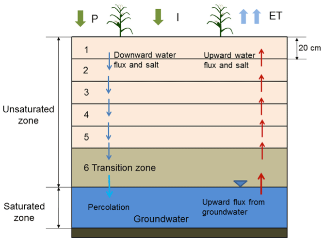
The moisture content and salt content are calculated for each day (Fig. 1). All flow takes place within the day, and the water and salt content are in “equilibrium” (i.e., fluxes are zero) at the end of the day for which the calculations are made. Daily fluxes considered in the vadose model are the following: at the surface, the fluxes are irrigation, both irrigation water, I(t), and salt, S0(t), and precipitation, P(t), and for each layer, j, on days with irrigation and rainfall, the downward flux of water, Rw(j, t), and salt, S(j, t), between the layers. On days without water input at the soil surface, an upward groundwater flux U(j, h, t) and salt S(j, t) are considered. The flux to the surface depends on the groundwater depth. Finally, transpiration, T(j, t), removes water from the layers with roots of the crops and evaporation, E(j, t), from all layers.
The EPICS model consists of two modules: the VADOSE module and the CROP module. The two modules are linked through the evapotranspiration flux in the soil (Fig. 2).
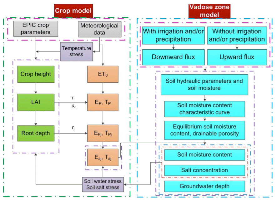
Figure 2Schematic diagram of the linked novel Shallow Aquifer-Vadose zone surrogate module and EPIC module. Note: ET0 is the reference evapotranspiration, Ep and Tp are the potential evaporation and potential transpiration, Ea and Ta are the actual evaporation and actual transpiration, Kc is the crop coefficient, τ is the development stage of the leaf canopy, and rj is the root function of soil layer j.
The CROP module employs functions of the EPIC model (Williams et al., 1989) and root growth distribution (Novak, 1987; Kendy et al., 2003; Chen et al., 2019). The CROP module calculates daily values of crop height, root depth, and leaf area index (LAI) based on climatic data (Fig. 2).
The VADOSE module calculates the moisture and salt content in the root zone and the upward movement of the groundwater (Fig. 2). Field capacity varies with depth and is a function of the (shallow) groundwater depth and the soil characteristic curve (Liu et al., 2019). Moisture contents become less than field capacity when the upward flux is less than the actual evapotranspiration.
Finally, the link between the VADOSE and CROP modules is achieved by calculating the actual evapotranspiration with parameters of both modules consisting of the moisture content and salt content simulated in the VADOSE module and the root distribution and potential evapotranspiration in the CROP module (Fig. 2).
2.3 Theoretical background of the EPICS model
In the next section, the equations of the CROP in the VADOSE modules are presented. The calculations are carried out sequentially on a daily time step. This model predicts field daily soil water, salt content, and crop growth, which are critical parameters for irrigation water management. For field and regional water management and irrigation policy development, resolution of the daily time step is sufficient. Finer resolution is not needed for managing water and salt content for irrigation. In the first step, the actual evaporation and transpiration are calculated for each layer in the model. Next, the moisture content and salt content are adjusted for the various fluxes. Since the equations for the downward movement on days of rainfall and/or irrigation are different than for upward movement from the groundwater on the remaining days, we present the upward and downward movement in separate sections. The code was written in Matlab 2014Ra and Microsoft Excel was used for data input and output.
2.3.1 CROP module
The crop module uses functions of EPIC (Williams et al., 1989) to calculate LAI, crop height and the root depth (green boxes in Fig. 2), the potential transpiration, Tp, and evaporation, Ep (orange boxes in Fig. 2). Input data for the CROP module included mean daily temperature (Tmean), maximum daily temperature (Tmx), minimum daily temperature (Tmn), maximum crop height (Hmx), maximum LAI (LAImx), maximum root depth (RDmx), dimensionless canopy extinction coefficient (Kb), and total potential heat units required for crop maturation (PHU).
The potential rates of evaporation, EP(j, t), and transpiration, TP(j, t), of different layers are derived from the total rates and a root function that determines the distribution of roots in the vadose zone:
where j is the number of soil layers and t is the day number, TP(t) is the total potential transpiration, and EP(t) is the total potential evaporation at time, t. Both are calculated with the CROP module (Sect. S1 in the Supplement). Root functions (Sau et al., 2004; Delonge et al., 2012) were used to calculate transpiration and evaporation of different soil layers. rT(j, t) is the root function for the transpiration and rE(j, t) is the root function for the evaporation. Both have the same general equation but with a different value for the constant δ.
where z1j is the depth of the upper boundaries of the soil layer j. For rT(j, t), if the root depth is smaller than the lower boundaries of the soil layer j, Z2j is equal to the root depth, and if the root depth is greater than the lower boundaries of the soil layer j, Z2j is the depth of the lower boundaries of the soil layer j. For rE(j, t), Z2j is the depth of the lower boundaries of the soil layer j. Zr is the root zone depth, and δ is the water use distribution parameter. Note that the sum of rT(j, t) of all soil layers is equal to 1. In the study of Novark (1987), the value of δ for corn is 3.64, and we used this value. To obtain rE(j, t), δ was set to 10 (Chen et al., 2019; Kendy et al., 2003). Sunflower root function simulation employed the same δ values as for maize.
The actual evaporation rates, Ea(j, t), and transpiration, Ta(j, t), for each soil layer, j, at time, t, are calculated as a proportion of the potential values as
where kE(j) and kT(j) are water stress coefficients and S(j) is a salt stress coefficient. According to Raes et al. (2009), the water stress coefficients are
where θfc(j) is the moisture content at field capacity for layer j, or when the conductivity becomes limiting and θr(j) is the moisture content at wilting point, θ(j, t) is the soil moisture content for layer j at time t.
Then the water stress coefficient in Eq. (3b) is
where fshape is the shape factor of the kT(j ,t) curve and p is the fraction of readily available soil water relative to the total available soil water. Finally, the salt stress coefficient S(j, t) for each layer in Eq. (3b) can be calculated as (Allen et al., 1998; Xue et al., 2018)
where ky is the factor that affects the yield, ECe is the electrical conductivity of the soil saturation extract (mS cm−1), ECethreshold is the calibrated threshold of the electrical conductivity of the soil saturation extract when the crop yield becomes affected by salt (mS cm−1), and B is the calibrated crop-specific parameter that describes the decrease rate of crop yield when ECe increases per unit below the threshold. The electrical conductivity of the soil saturation extract can be calculated as (Rhoades et al., 1989)
where EC1:5 is the electrical conductivity of the soil extract of soil samples mixed with distilled water in a proportion of 1:5.
2.3.2 VADOSE module
To model the daily soil moisture content and groundwater depth, first we need to calculate the soil moisture content at field capacity and the drainable porosity based on the soil moisture characteristic curve. Besides, we assume that the water and salt move downward on rainy and/or irrigation days, while the water and salt move upward on days without rain and/or irrigation.
Parameters based on the soil moisture characteristic curve for modeling
Moisture content at field capacity
Field capacity with a shallow groundwater is different than in soils with deep groundwater where water stops moving when the hydraulic conductivity becomes limiting at −33 kPa. When the groundwater is shallow, the hydraulic conductivity is not limiting and the water stops moving when the hydraulic potential is constant, and thus the matric potential is equal to the height above the water table (Gardner, 1958; Gardner et al., 1970a, b; Steenhuis et al., 1988; Liu et al., 2019). Assuming a unique relationship between moisture content at field capacity and matric potential (i.e., soil moisture characteristic curve), the moisture content at field capacity at any point above the water table is a unique function of the water table depth. Thus, any water added above field capacity will drain downward. When the groundwater is recharged, the water table will rise and increase the moisture contents at field capacity throughout the profile.
The moisture contents at field capacity were found by Liu et al. (2019) using the simplified Brooks and Corey soil moisture characteristic curve (Brooks and Corey, 1964):
in which θ is the soil moisture content (cm3 cm−3), θs is the saturated moisture content (cm3 cm−3), φb is the bubbling pressure (cm), φm is the matric potential (cm), and λ is the pore size distribution index. The moisture content at field capacity, θfc(z, h), for any point, z, from the surface water for a groundwater at depth, h, can be expressed as (Liu et al., 2019)
where h (cm) is the depth of the groundwater and z (cm) is the depth of the point below the soil surface. Thus (h−z) is the height above the groundwater, and this is equal to the matric potential for soil moisture content at field capacity.
For shallow groundwater, the matric potential at the surface is −33 kPa when the groundwater is at 3.3 m depth. For this matric potential, as mentioned above, the conductivity becomes limiting. This depth of the groundwater is therefore the lower limit over which the VADOSE module is valid.
Evapotranspiration can lower the soil moisture content below field capacity. Thus, the maximum moisture content in the VADOSE module is determined by the soil characteristic curve and the height of the groundwater table, and the minimum is the wilting point that can be obtained by evapotranspiration by the crop. Note that the saturated hydraulic conductivity does not play a role in determining the moisture content because inherently it is assumed that it is not limiting in the distribution of the water.
Drainable porosity
The drainable porosity is a crucial parameter in modeling the groundwater depth and soil moisture content. According to the soil water characteristic curve at field capacity, the drainable porosity can be expressed as a function of the depth. The drainable porosity is obtained by calculating the field capacity Wfc(h) (cm) for each layer at all groundwater depths. The total water content at field capacity of the soil profile over a prescribed depth with a water table at depth h can be expressed as
where θfc(j, h) is the average moisture content at field capacity of layer j that can be found by integrating Eq. (8) from the upper to lower boundaries of the layer and dividing by the length L(j), which is the height of layer j. The matric potential at the boundary is equal to the height above the water table. The drainable porosity, μ(h), which is a function of the groundwater depth h, can simply be found as the difference in water content when the water table is lowered over a distance of 2Δh.
where Δh=0.5 L(j) (cm).
Downward flux (at times of irrigation and/or precipitation) and model output
During the downward flux period, the upward water flux from groundwater is zero. Under this condition, the model can output the daily soil moisture content of different soil layers, the percolation from each soil layer to the soil layer beneath, the discharge from soil water to groundwater, the salt concentration of groundwater and of soil water in each soil layer, and the groundwater depth.
Water
A downward flux occurs when either the precipitation or irrigation is greater than the actual evapotranspiration. In this case, upward flux will not occur because the actual evapotranspiration is subtracted from the input at the surface. We consider two cases when the groundwater is being recharged and when it is not.
When the net flux at the surface (irrigation plus rainfall minus actual evapotranspiration) is greater than that needed to bring the soil up to equilibrium moisture content, the groundwater will be recharged and the distance of the groundwater to the soil surface decreases, and the moisture content will be equal to the moisture at field capacity. The fluxes from one layer to the next can be calculated simply by summing the amount of water needed to fill up each layer below to the new moisture content at field capacity. Hence, the percolation to groundwater, Rgw(t), can be expressed as
where n is the total number of layers, θ(j, t) is the average soil moisture content on day t of layer j (cm3 cm−3), Ea(t) is the actual evaporation (mm), Ta(t) is the actual transpiration (mm), P(t) is the precipitation (mm), and I(t) is the irrigation (mm).
When the groundwater is not recharged, the rainfall and the irrigation are added to the uppermost soil layer and when the soil moisture content will be brought up to the field capacity and the excess water will infiltrate to the next soil layer, bringing it up to field capacity. This process continues until all the rainwater is distributed. Formally the soil moisture can be expressed as
where θ(j, t) is the average soil moisture content on day t of layer j (cm3 cm−3); Rw(j−1, t) is the percolation rate to layer j (mm) and can be found with Eq. (12) by replacing j−1 for n in the summation sign.
For the uppermost soil layer, the water percolation can be expressed as
Salinity
The salt concentration for layer j can be expressed by a simple mass balance as
where C(j, t) is the salt concentration of layer j at time t (g L−1). The equation can be rewritten as an explicit function of C(j, t):
For the surface layer j=1, we obtain
where CI is the salt concentration in the irrigation water (g L−1).
The salt concentration of the groundwater Cgw(t) can be estimated as
where C(5, t) is the soil salinity concentration of the soil layer 5 on day t (g L−1), G(t−1) is the difference of the groundwater depth and the depth of the largest groundwater table fluctuation depth of the groundwater table on day (t−1) (m) (Xue et al., 2018), and Cgw(t) is the soluble salt concentration of groundwater at day t (g L−1).
Upward flux and model output
For the upward flux period, the downward water flux to groundwater is zero. The evapotranspiration leads to the decrease in soil moisture content in the vadose zone and lowers the groundwater table due to the upward movement of groundwater to crop root zone and soil surface. The soil moisture content is calculated by taking the difference of equilibrium moisture content associated with the change in groundwater depth. Under this condition, the model can output the daily soil moisture content of different soil layers, the upward groundwater flux, the groundwater depth, and the salt concentration of groundwater and of soil water in each soil layer.
Water
The groundwater upward flux Ugw(h, t) is limited by either the maximum upward flux of groundwater Ugw,max(h) or the actual evapotranspiration, formally stated as
where Ugw,max(h, t) is the actual upward flux from groundwater (mm), Ea(t) is the actual evaporation at day t (mm), Ta(t) is the actual transpiration at day t (mm), Ea(j, t) is the actual evaporation at day t of layer j (mm), and Ta(j, t) is the actual transpiration at day t of layer j (mm).
The maximum upward flux can be expressed as (Liu et al., 2019; Gardner et al., 1958)
where a and b are constants that need to be calibrated and h is the groundwater depth (cm).
Two cases are considered for determining the moisture contents of the layers depending on whether the actual evapotranspiration is greater or less than the maximum upward flux.
-
Case I: : in this case, where the maximum upward flux is greater than the evaporative demand, the groundwater depth is updated:
where is the average drainable porosity over the change in groundwater depth h. The moisture content after the change in groundwater depth becomes
Note that when the layer is at field capacity and the upward flux is equal to the evaporative flux, the layer remains at field capacity for the updated groundwater depth at time t.
-
Case II: : in this case, the groundwater depth is updated:
When the upward flux is less than the sum of the actual evaporation and transpiration, the moisture content is updated with the difference between the two fluxes, Ugw,max(h) and [Ea(t)+Ta(t)], according to a predetermined distribution extraction of water out of the root zone:
The upward flux of water can be found by summing the differences in moisture content above the layer j similar to Eq. (14), but starting the summation at the groundwater.
Salinity
The salt from groundwater is added to the soil layers according to the root function. The soil salinity concentration in layer j at day t can be expressed as
Since water is extracted from the reservoir that has the same concentration as in the reservoir, the concentration will not change; hence, the equation used to estimate the groundwater salt concentration can be expressed as
3.1 Study area
Field experiments were conducted in 2017 and 2018 in Shahaoqu experimental station in Jiefangzha sub-district, Hetao irrigation district in Inner Mongolia, China (Fig. 3). Irrigation water originates from the Yellow River. The change in the irrigation water salinity is small and can be ignored during the crop growth period. The area has an arid continental climate. Mean annual precipitation is 155 mm a−1, of which 70 % falls from June to September. Pan evaporation is 2000 mm a−1 (Xu et al., 2010). The mean annual temperature is 7 ∘C. The soils begin to freeze in the middle of November and to thaw at the end of April or beginning of May. Maize, wheat, and sunflower are the main crops in Jiefangzha sub-district and are grown with flood irrigation. The groundwater depth is between 0.5 and 3 m. Regional exchange of groundwater is minimal due to the low gradient of 0.01–0.025 (Xu et al., 2010). Thus, the groundwater flows mainly vertically with minimum lateral flow in the regional scale. Over 50 % of the total irrigated cropland, 5250 km2 in the Hetao irrigation district in the Yellow River basin, is affected by salinity (Feng et al., 2005).

Figure 3Location of the Shahaoqu experimental field. (Note: the figure was downloaded from © Google Earth. The imagery was taken on 8 April 2019.)
3.2 Field observations and data
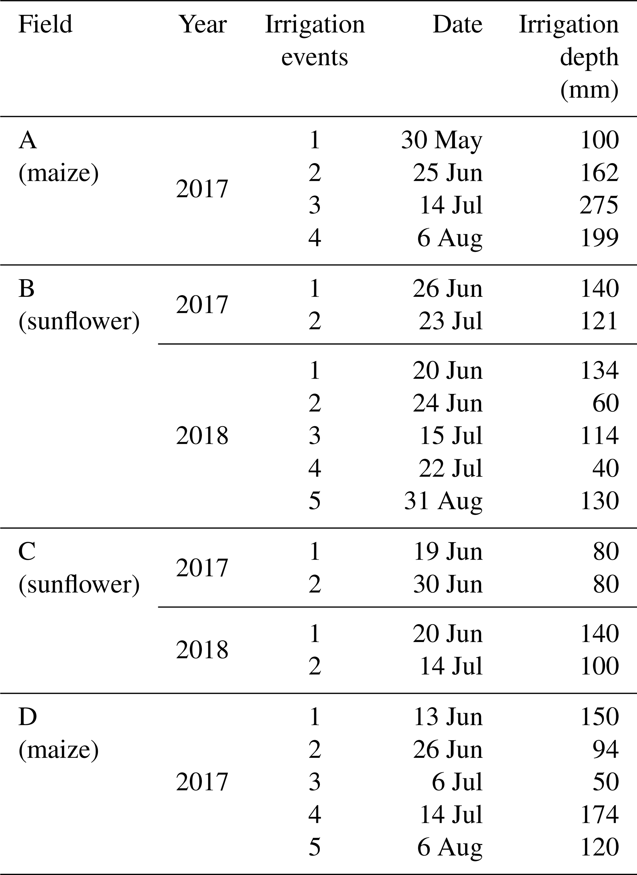
The layout of the experimental fields is shown in Fig. 3. The areas of fields A–D are 920, 2213, 1167, and 1906 m2, respectively. Fields A and D were planted with maize on 10 May and harvested on 30 September 2017. In 2018, fields A and D were planted with gourds and were therefore not monitored in 2018. Fields B and C were seeded with sunflower in both 2017 and 2018. The sunflower was planted on 1 June 2017 and 5 June 2018. Harvest was on 15 September in both years. The fields were irrigated by flooding the field ranging from two to five times during the growing season (Table 1). The salinity of the irrigation source water was measured three times during the crop growth period and the mean value was used in the mass balance. The salinity of the irrigation source water is assumed unchanged. A well was installed in each experimental field to monitor the groundwater depth.
Table 1Irrigation scheduling for the Shahaoqu experimental fields in 2017 and 2018.
Daily meteorological data, including air temperature, precipitation, relative humidity, wind speed, and sunshine duration, originated from the weather station at the Shahaoqu experimental station. The soil moisture content for the four experimental fields in 2017 and for field C in 2018 during the crop growing season was measured every 7–10 d at the depths of 0–20, 20–40, 40–60, 60–80, and 80–100 cm by taking soil samples and oven drying. In 2018, in addition, the soil moisture content at the same depths was monitored daily using Hydra Probe Soil Sensors (Stevens Water Monitoring System Inc., Portland, OR, USA) in field B except the oven drying method. The Hydra Probe was calibrated using the intermittent manual measurements. In 2017, the groundwater depths were manually measured in all four experimental fields about every 7–10 d. In 2018, the groundwater depth in fields B and C was recorded at 30 min intervals using an HOBO Water Level Logger-U20 (Onset, Cape Cod, MA, USA). The sensors of the soil moisture content and groundwater depth were connected to data loggers and downloaded via wireless transmission. The crop leaf area and crop height were manually measured every 7–12 d.
Undisturbed soil samples were collected in 5 cm high rings with a diameter of 5.5 cm from the five soil layers where the soil moisture was taken and used for textual analysis, saturated soil moisture content, field capacity, and soil bulk density. The soil texture was analyzed with a laser particle size analyzer (Mastersizer 2000, Malvern Instruments Ltd., United Kingdom). The American soil texture classification method was used in this study. Finally, the soil samples were collected 7–10 d apart to monitor the change in electrical conductivity (EC). The soil samples were mixed with distilled water in a proportion of 1:5 to measure the electrical conductivity of the soil water by a portable conductivity meter. It is assumed that 1 ms cm−1 corresponds to 640 mg L−1 of the total dissolved salts (Wallender and Tanji, 2011; Xue et al., 2018).
3.3 Model calibration and validation
The observed soil moisture contents, groundwater depths, crop heights, LAIs, and salinity concentrations for field A with maize and sunflower fields B and C in 2017 were used for calibration, and the sunflower data of fields B and C in 2018 and the maize data in field D in 2017 were used for validation. The initial θfc was based on the measured data (Table 2). The initial values of θs and θr were derived from the soil texture with the method of Ren et al. (2016) (Table 2). The default values of EPIC for sunflower and maize were used as initial values for simulating crop growth (Kcmax and LAImx in Eq. S3, Kb in Eq. S4, Hmx in Eq. S7, PHU in Eq. S9, Tb in Eq. S10, ad in Eq. S12, T0 and Tb in Eq. 16, and RDmx in Eq. S18). The initial value maximum crop coefficient (Kcmax) in Eq. (S3) in Sect. S1 for evapotranspiration calculation was taken from Sau et al. (2004). The initial values of two groundwater parameters (a and b in Eq. 23) were based on Liu et al. (2019). The Brooks and Corey soil moisture characteristic parameters (φb, λ in Eq. 8) were obtained by fitting the outer envelope of the measure moisture content and water table data.
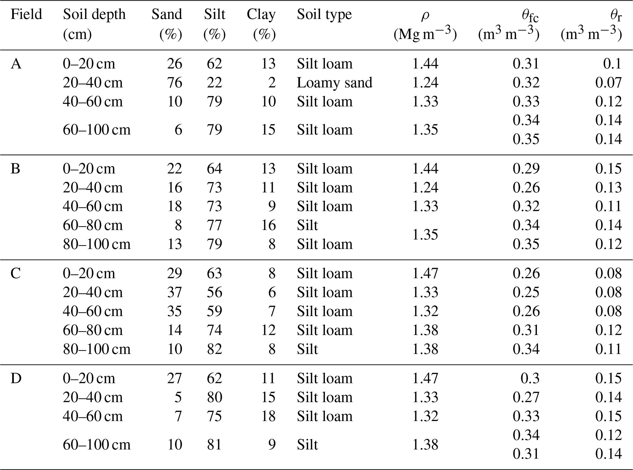
Table 2Soil texture and bulk density of the experimental fields in Shahaoqu.
Statistical indicators were used to evaluate goodness of fit of the hydrological model for both calibration and validation (Ritter and Muñoz-Carpena, 2013). The statistical indicators included the root mean square error (RMSE) (Abrahart and See, 2000),
the mean relative error (MRE) (Dawson et al., 2006; Nash and Sutcliffe, 1970),
the Nash–Sutcliffe efficiency coefficient (NSE) (Nash and Sutcliffe, 1970),
and the determination coefficient (R2) and regression coefficient (b) (Xu et al., 2015)
where N is the total number of observations; Pi and Oi are the ith model predicted and observed values (i=1, 2, 3 … N), respectively; and are the mean observed values and predicted values, respectively. The RMSE is used to evaluate the bias of the measured data and predicted data. The MRE can evaluate the credibility of the measured data. The NSE is usually used to evaluate the quality of the hydrological models. The R2 is used to measure the fraction of the dependent variable total variation that can be explained by the independent variable. And the regression coefficient represents the influence of the independent variable on the dependent variable in the regression equation. The values of RMSE and MRE close to 0 indicate good model performance. The value of NSE ranges from −∞ to 1. NSE = 1 means a perfect fit, while the negative NSE values indicate the mean observed value is a better predictor than the simulated value (Moriasi et al., 2007). For b and R2, the value closest to 1 indicates good model predictions.
3.4 Parameter sensitivity analysis
A sensitivity analysis was performed to determine how the input parameters affected output of the models (Cloke et al., 2008; Cuo et al., 2011). Each parameter was varied over a range of −30 % to 30 % to derive the corresponding impact on the model output of soil moisture, groundwater depth, soil salinity, leaf area index, and actual evapotranspiration. The change in output values was plotted against the change in input values.
The 2017 and 2018 experimental data of the Shahaoqu farmers' fields in the Hetao irrigation district (Fig. 3) are presented first, followed by the calibration and validation results of the CROP and VADOSE modules of the EPICS model.
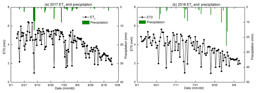
Figure 4Reference evapotranspiration (ET0) and precipitation during the crop growth period in 2017 and 2018.
4.1 Results of the field experiment
4.1.1 Water input
The precipitation was 63 mm in 2017 (10 May to 30 September) and 108 mm in 2018 (1 June to 15 September). The precipitation from the greatest rainstorm was 26 mm on 1 September 2018 (Fig. 4). Irrigation provided most of the water for the crops. Field A (maize) was irrigated four times for a total of 736 mm and field D (maize) was irrigated five times for a total of 588 mm in 2017. Sunflower fields B and C were both irrigated twice with total water amounts of 261 and 160 mm, respectively, in 2017. In 2018, fields B and C were irrigated five and two times, respectively, with total water amounts of 478 and 240 mm, respectively. The reference evapotranspiration ranged from 1 mm d−1 to a maximum of 6.4 mm d−1 during the crop growing period (Fig. 4). The total reference evapotranspiration from 10 May to 30 September 2017 was 595 and 368 mm from 1 June to 15 September 2018. The reason was that there were more rainfall days in June, July, and September in 2018 than in 2017, which increased the amount of water available for the evapotranspiration by the crop in 2018. In addition, the wind speed was high so that the increase in the evapotranspiration was elevated. In the studies of Ren et al. (2017) and Miao et al. (2016), the mean ET0 was over 6 mm per day in May. Hence, the ET0 during the study period in 2017 was greater than in 2018.
4.1.2 Soil physical properties
Based on the soil textural analysis in Table 2, the soils were classified as silt, silt loam, and loamy sand. Bulk densities varied from 1.24 to 1.47 Mg m−3, with the greatest bulk densities in the 0–20 cm soil layer. There was generally more sand in the top 40 cm than below. The subsoil was heavier and had the greatest percentage of silt (Table 2). The moisture content at −33 kPa (0.33 bar) varied from 0.25 to 0.35 cm3 cm−3 and at 1.5 Mpa (wilting point at 15 bar) ranged from 0.08 to 0.15 cm3 cm−3 (Table 2).
4.1.3 Soil moisture content
Moisture content, rainfall, and irrigation amounts are depicted for the five layers and the four fields in 2017 and two fields in 2018 in Fig. 5. Blue closed spheres indicate that the moisture content was determined on cored soil samples (Fig. 5a–c, e, and f) and close-spaced spheres when the hydra probe was used (Fig. 5d). The moisture contents were near saturation when irrigation water was added and subsequently decreased due to crop transpiration and soil evaporation (Fig. 5). In all cases, the moisture contents during the main growing period remained above the moisture content at −33 kPa that ranged from 0.25 to 0.34 cm3 cm−3 for the 60–80 cm depth (Table 2, Fig. 5). Only after the last irrigation and during harvest of the crop did the moisture content in the top 0–40 cm for maize and 0–60 cm for sunflower decrease below the moisture content at −33 kPa. During the growing season, the variation of moisture content was greater in the top 60 cm with the majority of the roots than in the lower depths where, after the first irrigation, it remained nearly constant close to saturation.
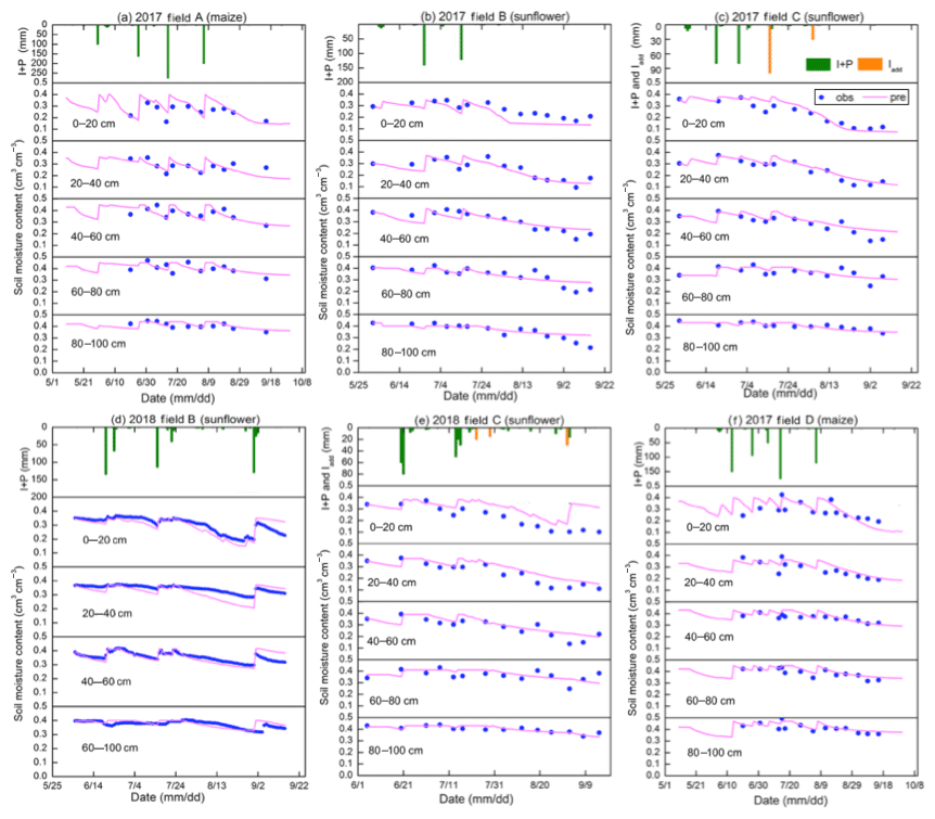
Figure 5Observed (blue dots) and simulated soil moisture content of the Shahaoqu experimental fields during model calibration (a–c) and validation (d–f).
4.1.4 Salinity
Overall the salt concentration is greatest at the surface and increases at all depths during the growing season. Sunflower is more salt tolerant than maize and the overall salt concentration was greater in the sunflower fields (Fig. 6) at comparable times of the crop development for field B but not for field C. Comparing the salt concentration and soil moisture patterns (Fig. 5), we note that they behave similarly but opposite to each other (Fig. 6). The soil salinity concentration was decreasing during an irrigation event due to dilution and then gradually increasing partly due to evaporation of the water. Some of the soil salt was transported to the layers below during irrigation and some salt was moving upward with the evaporation from the surface. As expected, after the harvest, the fall irrigation decreased the salt concentration from fall 2017 to spring 2018.

Figure 6Observed (blue dots) and simulated soil salinity concentration of the experimental fields in Shahaoqu during model calibration (a–c) and validation (d–f).
4.1.5 Groundwater observations
The variation in groundwater depth during the growing season was very similar for both years and in all fields. The groundwater depth for all fields was between 50 and 100 cm from the surface after an irrigation event and then decreased to around 150 cm before the next irrigation or rainfall (Fig. 7). Only after the last irrigation in August 2017 did the water table decrease to below 250 cm and to around 200 cm in 2018. Field D followed the same pattern, but the groundwater was more down from the surface. In several instances, the groundwater table increased without an irrigation or rainfall event in sunflower field C (Fig. 7c and e). This was likely related to an irrigation event either from an irrigation in a nearby field that affected the overall water table or an accidental irrigation that was not properly documented. We estimated the amount of irrigation water based on the change in moisture content in the soil profile (orange bars in Fig. 7c and e). Finally, there was a notable rise in the water table of a mean 375 mm “fall irrigation” after harvest between the end of 2017 (Fig. 7a–c) and the beginning of 2018 (Fig. 7d–f), which is a common practice in the Jiefangzha irrigation district to leach the salt that has accumulated in the profile during the growing periods.
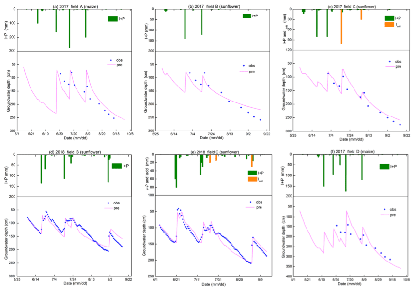
Figure 7Observed (blue dots) and simulated groundwater depth of the experimental fields in Shahaoqu during model calibration (a–c) and validation (d–f).
Note that in Fig. 7, after an irrigation event, the groundwater depth was between 50 and 80 cm, while the whole profile was saturated (Fig. 5). This is directly related to the bubbling pressure of the water. After the irrigation event stopped, the water table was likely at the surface but then immediately decreased because a small amount of evaporated water will bring the water table down to a depth of approximately equal to the bubbling pressure, φb, in Eq. (8). The bubbling pressures are listed in Table 3.
4.1.6 LAI and plant height
Plant height and LAI followed the typical growth curve that started slowly to rise in the beginning, accelerated during the vegetative stage, and then became constant during the seed setting and ripening stages (Fig. 8). In the maturing stage, the leaf area index decreased.
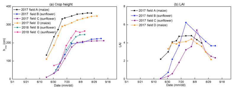
Figure 8Observed crop height (a) and leaf area index (b) of the experimental field in Shahaoqu in 2017 and 2018.
4.2 Soil moisture characteristic curve and drainable porosity
To simulate the soil moisture content and to derive drainable porosity as a function of water table depth, the soil moisture characteristic curves were derived by plotting the observed soil moisture content in 2017 and 2018 versus the height above the water table to the soil surface for the five soil layers in Fig. 9. The Brooks–Corey equation (Brooks and Corey, 1964) was fitted through the outer envelope of the points. The parameters of the Brooks–Corey equation were adjusted through trial and error to obtain the best fit (Table 3a). In Fig. 9, points on the left-hand side of the soil moisture characteristic curve (moisture content smaller than the field capacity) were due to water removal at times when evaporative demand was greater than the upward water flux. Under these conditions the conductivity is limiting in the soil and there is no relationship between groundwater depth and matric potential. Since we take the water table depth as a proxy for matric potential, these points are omitted when drawing the soil characteristic curve. The few points at the right of the soil moisture characteristic curve indicate the soil moisture was greater than field capacity and matric potential and groundwater were not yet at equilibrium after an irrigation event.

Figure 9Soil moisture characteristic curves of five soil layers in the experimental fields. The pink line is the fit with the Brooks–Corey equation.
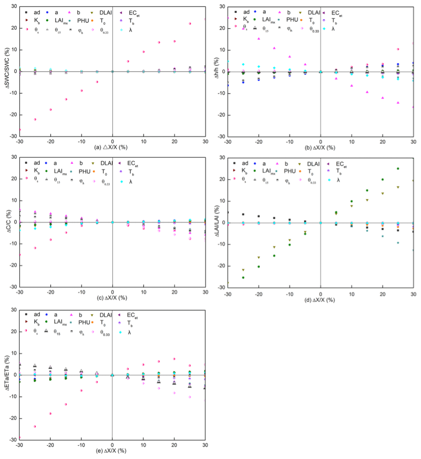
Figure 10Parameter sensitivity analysis for (a) soil moisture content, (b) groundwater depth, (c) salt salinity concentration, (d) LAI, and (e) ET.
The fitted parameter values are consistent. Field A had a greater bubbling pressure and moisture content at −33 kPa than the other fields, indicating that this field had more clay. This was confirmed by the data in Table 2. For fields B–D, the bubbling pressure was greater at the 60–80 cm depth or the 80–100 cm depth, which was also in accordance with the data in Table 2.
Table 3(a) Calibrated soil hydraulic parameters in the Brooks and Corey soil moisture characteristic curve. (b) Calibrated groundwater parameters.
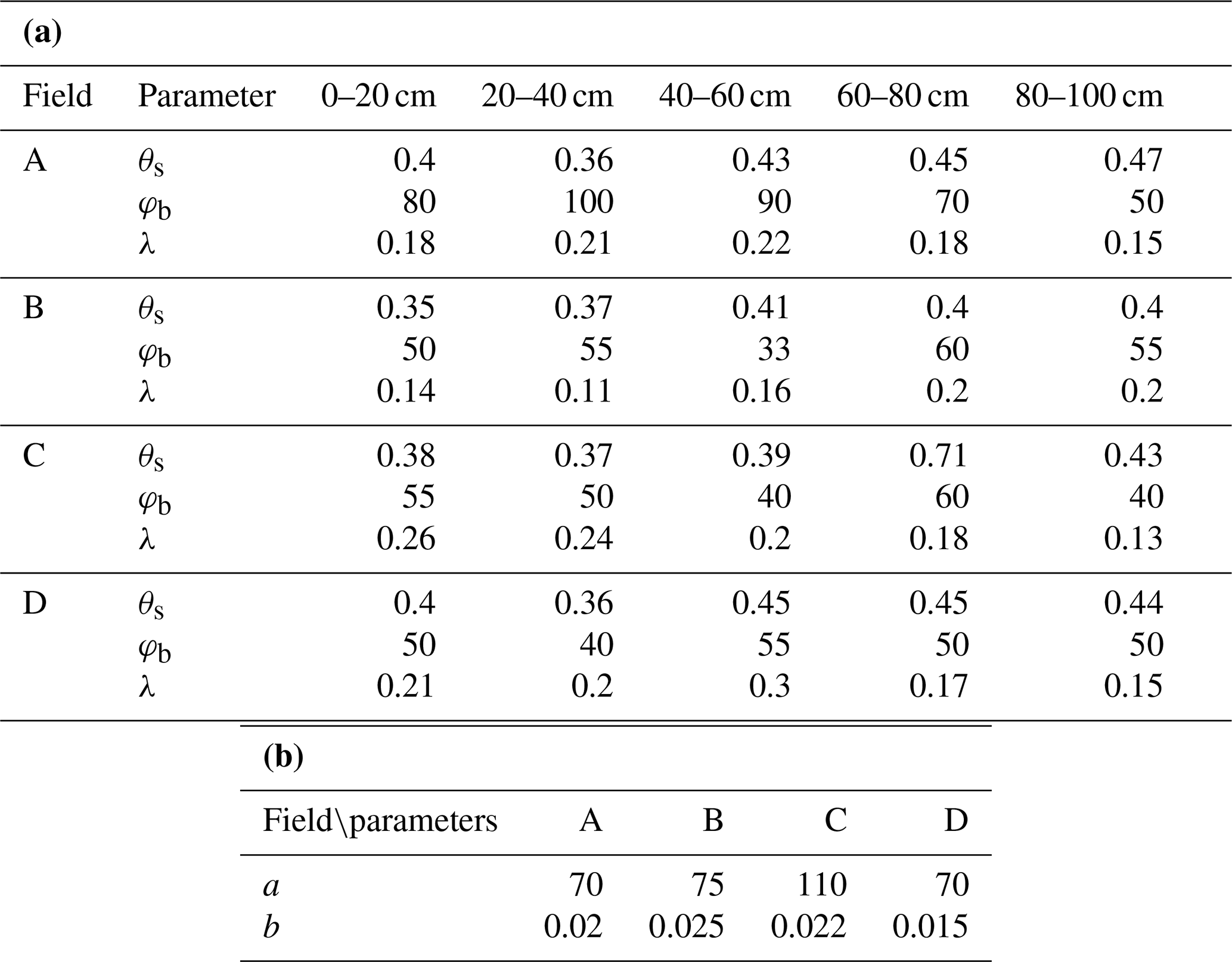
Note: θs is the soil moisture at saturation (cm3 cm−3), φb is bubbling pressure (cm), and λ is the pore size distribution index.
4.3 Parameter sensitivity analysis
The results of sensitivity analysis of the 15 input parameters on 5 output parameters are shown in Fig. 10. The evaluated output parameters are soil moisture content, groundwater depth, soil salinity concentration, field evapotranspiration, and crop LAI. Steeper lines indicate a greater sensitivity of the parameter.
The results of the sensitivity analysis show that moisture content predictions (Fig. 10a) are the most sensitive to the input value of the saturated moisture content (θs). None of the other parameters are very sensitive. This includes the shape parameters for the soil characteristic curve, bubbling pressure φb, and exponent λ. The input parameter with the most sensitivity to groundwater depth (Fig. 10b) is the saturated moisture content as well. Other less sensitive parameters are the exponent b and constant a in Eq. (23) in predicting the upward flux and the bubbling pressure, φb, of the soil moisture characteristic curve (Eq. 8a). Likewise, in the case of the salinity predictions (Fig. 10c), the saturated moisture content gives the greatest relative change in salt content. Less sensitive, but still important, are the field capacity, θfc, the bubbling pressure, φb, and the exponent λ of the soil characteristic curve (Eq. 8a) and b in Eq. (23). The sensitivity parameters for the leaf area index (LAI) (Fig. 10d) are the maximum potential leaf area index, LAImx, and fraction of the growing season when leaf area declines (DLAI) followed by total potential heat units required for crop maturation (PHU). Finally, for the evapotranspiration (Fig. 10e), the saturated soil moisture content is the most sensitive parameter, and other less sensitive parameters are the exponent b and field capacity.
Thus, the model output is most sensitive to the input parameters that define the soil hydraulic properties, groundwater flux, and crop growth. As expected, since the soil remains near field capacity, the parameters that relate to the reduction of evaporation when the soil dries out are insensitive. When used in the simulation practices, the model needs to be calibrated and verified to avoid high error from parameter uncertainty.
4.4 Model calibration and validation with field data
The model parameters were calibrated and validated using the observed moisture content, groundwater depth, plant height, leaf area index, and calculated evapotranspiration. The data of sunflower fields B and C and maize field A were collected and used for calibration. Since farmers did not grow maize in 2018, the 2017 data of maize field D, together with sunflower fields B and C in 2018, were used for validation. The optimal parameter set was determined using graphical similarity between observed and predicted results together with near-optimum performance of the statistical indicators while keeping all values within physically acceptable ranges.
As a way of reducing the number of parameters that needed to be calibrated, we initially selected one to three most sensitive parameters for each of the observed time series, starting with evapotranspiration (including LAI and crop height) and followed by moisture content, groundwater depth, and salt content in the soil. This cycle was repeated several times until changes became small. The last stage of the calibration consisted of fine-tuning the remaining least sensitive parameters.
To calibrate the parameters in the CROP module, we calculated evapotranspiration during the crop growth period with the observed soil moisture content and groundwater depth by the soil water balance method. In addition, we used the observed LAI measurements in 2017 and plant height in both 2017 and 2018. LAI was not measured in 2018. The DLAI, LAImx, and Hmx in the crop module were adjusted to fit the observed LAI and crop height values. In addition, we fitted the θfc moisture content to obtain a good fit of the evapotranspiration. The saturated moisture content values were not adjusted since they were already determined for fitting the soil characteristic curve. The exponent b and constant a in Eq. (23) were adjusted to fit the observed soil moisture content and groundwater depth.
4.4.1 Evapotranspiration, crop height, and leaf area index
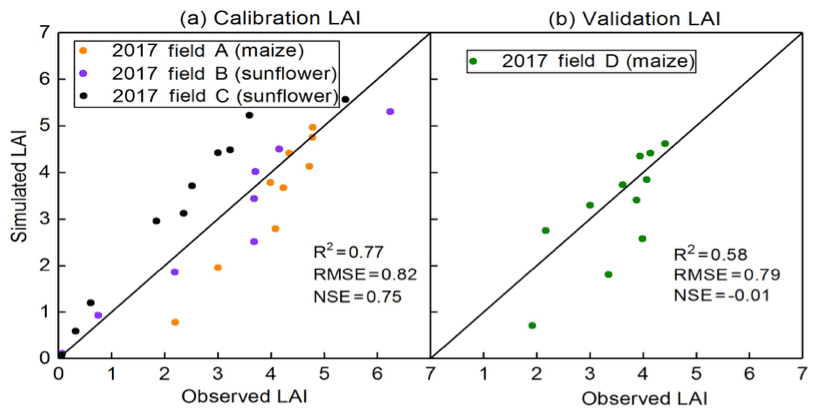
The predicted evapotranspiration and that calculated from the mass balance show a good agreement with Nash–Sutcliffe values ranging from 0.96 to 0.89 during calibration and validation (Fig. 11 and Table 4). The calibrated predictions of plant height fitted the observed values well during calibration and validation with Nash–Sutcliffe values ranging from 0.77 to 0.96 for the individual fields (Table 4) and over 90 % when the data were pooled for the fields during calibration and validation (Fig. 12). LAI was not measured in 2018. During calibration, Nash–Sutcliffe-predicted LAI values were good for sunflower but not as good for maize, but the coefficients of determination and slope in the regression were acceptable (Table 4, Fig. 13). In addition, the overall trend was predicted reasonably well (Fig. 13b).

Figure 11Comparison of predicted and observed actual evapotranspiration: (a) calibration and (b) validation.
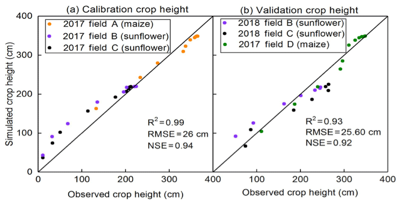
Figure 12Comparison of predicted and observed crop height: (a) calibration and (b) validation.
4.4.2 Soil moisture and groundwater depth
Next, the moisture contents and groundwater table were fitted with the parameters in the vadose model without changing the parameters in the CROP module. Saturated moisture content was the most sensitive parameter for calibrating the moisture content (Fig. 10a). Since this value was already determined a priori from the soil characteristic curve (Table 3a), we could not use other parameters to obtain a better fit since none were sensitive (Fig. 10a). Therefore, we calibrated the groundwater parameters (i.e., a and b parameters; Eq. 23) together with the moisture content to obtain the best fit for both. The fitted a and b values are listed in Table 3b. The fitted parameters between the four experimental fields were similar but not the same. This can be expected in river plains, where soils can vary over short distances.
Overall, the moisture contents were predicted well during calibration and validation (Figs. 5 and 14 and Table 4), with the exception of field B during validation (Table 4) with a NSE of 0.43. The moisture contents were predicted most accurately in the layers from 40 to 100 cm, where the soil moistures were at field capacity during most of the growing season (Fig. 14). In the top 40 cm, the predicted soil moisture content deviated from observed moisture contents, especially at the drier end (Figs. 5 and 14). Unlike at deeper depths, evapotranspiration determined the moisture contents at shallow depths. Prediction of evapotranspiration introduced additional uncertainties such as the distribution of the root system. This uncertainty is also likely the reason why the 2018 moisture contents during the validation are acceptable but not predicted as well as in 2017.

Figure 14Comparison of predicted and observed soil moisture content: (a) calibration and (b) validation.
The predicted and observed groundwater depths are in good agreement during both calibration and validation (Figs. 7 and 15). The MRE values were within ±10 % and the NSE values ranged from 0.52 for field D during validation to 0.91 in field C during calibration, where some of the recharge events were estimated (Table 4).

Figure 15Comparison of predicted and observed groundwater depth: (a) calibration and (b) validation.
Table 4Model error statistics for calibration and validation of models in 2017 and 2018 (mean relative error, MRE; root mean square error, RMSE; Nash–Sutcliffe efficiency, NSE; coefficient of determination, R2; regression coefficient).
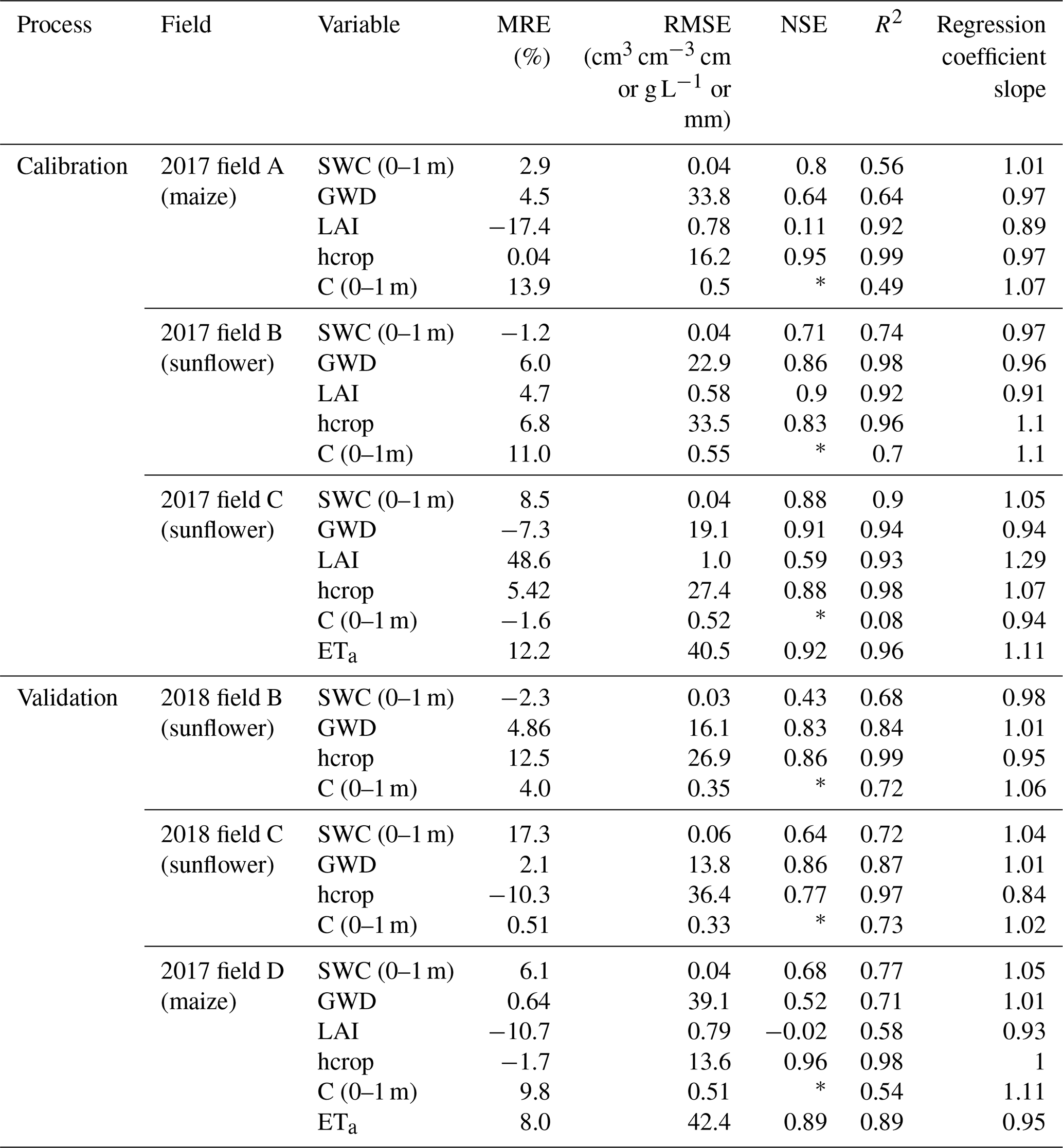
Note: * relative bias was over 5 %, invalidating the calculation of NSE. SWC is the soil moisture content, GWD is the groundwater depth, LAI is the leaf area index, hcrop is the height of the crop, C is the soil salinity concentration, and ETa is the actual evapotranspiration.
4.4.3 Soil salinity
The only parameter that could be adjusted each year for calibration of the salt concentrations was the initial salt concentration. The predicted salt concentrations in the top layers decreased after an irrigation event similar to the limited observed values (Fig. 6). Despite the salt concentration fitting visually reasonably well as shown in Figs. 6 and 16, there was a bias of 8 % in the data, and consequently the Nash–Sutcliffe efficiency could not be applied (Table 4) (Ritter and Muñoz-Carpena, 2013). Similarly to the moisture contents, the salt concentrations in the layers below 40 cm were predicted more accurately than the layers above 40 cm. More data should be collected during the whole year on the salt concentrations in the soil in order to accurately predict the salt concentrations.
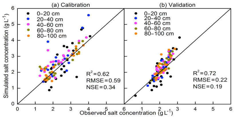
Figure 16Comparison of predicted and observed salt concentration during calibration (a) and validation (b).
The EPICS model is a surrogate model that can be applied in areas with shallow groundwater. It can simulate the soil moisture content and salt concentration for layers in the soil, the groundwater depth, upward movement of water from groundwater, evapotranspiration, and plant growth.
The model is different from traditional models that are based on the Richards equation; instead of calculating the fluxes first, in the EPICS model, the groundwater depth is calculated first based either on the amount of water removed by evapotranspiration on days without rain or irrigation or recharge to groundwater on the other days. Subsequently, when the groundwater is sufficiently shallow and the potential upward flux from the groundwater is greater than the evaporative demand, the moisture contents are adjusted so that soil moisture and groundwater depth are in equilibrium (i.e., field capacity). In this case, the matric potential is equal to the height above the water table, and the moisture contents can be found with the soil moisture characteristic curve. When the upward flux is less than the evaporative demand of the atmosphere and crop, the difference between the upward moisture content is determined by first decreasing the moisture content below the field capacity. The flux of water in the soil is then calculated based on the changes in water content. The advantage is fewer input parameters needed when compared with other numerical models (Šimůnek et al., 1998; Van Dam et al., 1997). For example, the hydraulic conductivity is not used in EPICS.
Although the uncertainties of field experimental observations and input data of the model affected the accuracy of simulation results, EPICS compares well with other models. Xu et al. (2015) tested SWAP-EPIC for two lysimeters grown with maize on the same experimental farm in the Hetao irrigation district where our experiment was carried out. The SWAP model solves the Richards equation numerically with an implicit backward scheme and is combined by Xu et al. (2015) with the EPIC model. The accuracy of our simulation results, despite the difference in complexity, is very similar. The moisture contents were simulated slightly better with EPICS, the groundwater depth was nearly the same, and the LAI values were predicted more accurately in the SWAP-EPIC model. Xu et al. (2015) did not simulate the salt content of the soil. Compared to fewer data and computationally intensive models that are applied in the Yellow River, the soil moisture content was simulated more accurately by EPICS than in the North China Plain, with 30 m deep groundwater by surrogate models of Kendy et al. (2003) and Yang et al. (2015a, b) and in the Hetao irrigation district by Gao et al. (2017b) and Xue et al. (2018) during the crop growth period.
To obtain more accurate results in the future, the upward capillary flux from groundwater needs to be improved. The salinity of irrigation source water also needs to be measured, especially for the areas irrigated by groundwater or the hydrologically closed basins. In addition, the evapotranspiration measured independently, using eddy covariance (Zhang et al., 2012; Armstrong et al., 2008) and the Bowen ratio–energy balance method (Zhang et al., 2007), should be further used to test the performance of the model in future study.
The limitation of the EPICS model is it can only be applied in areas where groundwater is generally less than 3.3 m deep. When the groundwater is deeper than 3.3 m, the field capacity of the surface soil is determined by the moisture content when the hydraulic conductivity becomes limiting and not by the depth of the groundwater.
Overall, the present model has the advantage that it greatly simplifies the calculation of the moisture content, groundwater depth, and salt content and, despite that, gives results similar to or better than other models applied in the Yellow River basin.
A novel surrogate field hydrological model called Evaluation of the Performance of Irrigated Crops and Soils (EPICS) was developed for irrigated areas with shallow groundwater. The model was tested with 2 years of experimental data collected by us for sunflower and 1 year of maize on replicated fields in the Hetao irrigation district, a typical arid to semi-arid irrigation district with a shallow aquifer. The EPICS model uses the soil moisture characteristic curve, upward capillary flux, and groundwater depth to derive the drainable porosity and predict the soil moisture contents and salinity. The evaporative flux is calculated with equations in EPIC (Erosion Productivity Impact Calculator) and the root distribution equation.
The simulation results show that the EPICS model can predict the soil moisture content and salt concentration in different soil layers, groundwater depth, and crop growth on a daily time step with acceptable accuracy during calibration and validation. The saturated soil moisture content is the most sensitive parameter for soil moisture content, salt concentration, and ET in our model.
In the future, the model should be tested in other areas with shallow groundwater that can be found in surface-irrigated sites and in humid climates in river plains. Once fully tested, the EPICS model can be used for optimizing water use on the local scale but, more importantly, on a watershed scale in closed basins where every drop of water counts.
| ET0 | Reference evapotranspiration (mm) | |
| p | Fraction of readily available soil water relative to the total available soil water (–) | |
| ETP | Potential evapotranspiration (mm) | |
| S | Salt stress coefficient (–) | |
| Ep | Potential evaporation (mm) | |
| B | Crop-specific parameter (%) | |
| Tp | Potential transpiration (mm) | |
| ky | Factor that affects crop yield (–) | |
| Ea | Actual evaporation (mm) | |
| ECe | Electrical conductivity of the soil saturation extract (mS cm−1) | |
| Ta | Actual transpiration (mm) | |
| ECethreshold | Threshold of the electrical conductivity of the soil saturation extract when the crop yield becomes affected | |
| by salt (mS cm−1) | ||
| Kc | Crop coefficient (–) | |
| EC1:5 | Electrical conductivity of the soil extract that soil samples mixed with distilled water in a proportion of | |
| 1:5 (mS cm−1) | ||
| τ | Development stage of the leaf canopy (–) | |
| θs | Soil moisture content at saturation (cm3 cm−3) | |
| rT | Root function for transpiration (–) | |
| φb | Bubbling pressure (cm) | |
| rE | Root function for evaporation (–) | |
| φm | Matric potential (cm) | |
| j | Number of soil layer (–) | |
| λ | Pore size distribution index (–) | |
| LAI | Leaf area index (–) | |
| h | Groundwater depth (cm) | |
| Tmean | Mean daily temperature (∘C) | |
| z | Depth of the point below the soil surface (cm) | |
| Tmx | Maximum daily temperature (∘C) | |
| Wfc(h) | Total water content at field capacity of the soil profile over a prescribed depth (cm) | |
| Tmn | Minimum daily temperature (∘C) | |
| L(j) | Height of layer j (cm) | |
| LAImx | Maximum leaf area index (–) | |
| μ | Drainable porosity (–) | |
| RDmx | Maximum root depth (cm) | |
| P | Precipitation (mm) | |
| Kb | Dimensionless canopy extinction coefficient (–) | |
| I | Irrigation (mm) | |
| PHU | Total potential heat units required for crop maturation (∘C) | |
| n | Number of soil layers (–) | |
| Z1j | Depth of the upper boundaries of soil layer j (cm) | |
| Rgw | Percolation to groundwater (mm) | |
| Z2j | Depth of the lower boundaries of the soil layer for rE(j, t); root depth or the lower boundaries of the soil | |
| layer for rT(j, t) (cm) | ||
| Rw(j−1, t) | Percolation rate to layer j from layer j−1 at day t (mm) | |
| δ | Water use distribution parameter (–) | |
| C(j, t) | Salt concentration of layer j at day t (g L−1) | |
| kE | Water stress coefficient for evaporation (–) | |
| CI | Salt concentration of irrigation water (g L−1) | |
| kT | Water stress coefficient for transpiration (–) | |
| Cgw | Salt concentration of groundwater (g L−1) | |
| θ | Soil moisture content (cm3 cm−3) | |
| Ugw | Actual upward flux of groundwater (mm) |
| θfc | Soil moisture content at field capacity (cm3 cm−3) | |
| Ugw,max | Maximum upward flux of groundwater (mm) | |
| θr | Soil moisture content at wilting point (cm3 cm−3) | |
| a | Constant used for calculation of Ugw,max (–) | |
| fshape | Shape factor of kT curve (–) | |
| b | Constant used for calculation of Ugw,max (–) |
The observed data used in this study are not publicly accessible. These data have been collected by personnel of the College of Water Resources and Civil Engineering, China Agricultural University, with funds from various cooperative sources. Anyone who would like to use these data should contact Zhongyi Liu, Xianghao Wang, and Zailin Huo to obtain permission.
The supplement related to this article is available online at: https://doi.org/10.5194/hess-24-4213-2020-supplement.
LZ and XW collected the data. ZL, ZH, CW, GH, XX, and TS contributed to the development of the model. The simulations with the model were done by ZL, ZH, and TS. Preparation and revision of the paper were done by ZL under the supervision of TS and ZH.
The authors declare that they have no conflicts of interest.
Peggy Stevens helped greatly with polishing the English. We thank the technicians in the Shahaoqu experimental station who helped in collecting data.
This research has been supported by the National Key Research and Development Program of China (grant nos. 2016YFC0400107 and 2017YFC0403301) and the National Natural Science Foundation of China (grant nos. 51639009 and 51679236).
This paper was edited by Alberto Guadagnini and reviewed by two anonymous referees.
Abrahart, R. J. and See, L.: Comparing neural network and autoregressive moving average techniques for the provision of continuous river flow forecasts in two contrasting catchments, Hydrol. Process., 14, 2157–2172, 2000.
Allen, R.G., Pereira, L.S., Raes, D., and Smith, M.: Crop evapotranspiration, Guidelines for computing crop water requirements – FAO Irrigation and Drainage Paper 56, FAO, Rome, 1998.
Armstrong, R. N., Pomeroy, J. W., and Martz, L. W.: Evaluation of three evaporation estimation methods in a Canadian prairie landscape, Hydrol. Process., 22, 2801–2815, https://doi.org/10.1002/hyp.7054, 2008.
Asher, M. J., Croke, B. F. W., Jakeman, A. J., and Peeters, L. J. M.: A review of surrogate models and their application to groundwater modeling, Water Resour. Res., 51, 5957–5973, https://doi.org/10.1002/2015WR016967, 2015.
Babajimopoulos, C., Panoras, A., Georgoussis, H., Arampatzis, G., Hatzigiannakis, E., and Papamichail, D.: Contribution to irrigation from shallow water table under field conditions, Agr. Water Manage., 92, 205–210, https://doi.org/10.1016/j.agwat.2007.05.009, 2007.
Blanning, R. W.: Construction and Implementation of Metamodels, Simulation, 24, 177–184, https://doi.org/10.1177/003754977502400606, 1975.
Brooks, R. H. and Corey, A. T.: Hydraulic properties of porous media, Hydrology Paper 3, Colorado State University, Fort Collins, Colorado, 37 pp., 1964.
Chen, C., Wang, E., and Yu, Q.: Modelling the effects of climate variability and water management on crop water productivity and water balance in the North China Plain, Agr. Water Manage., 97, 1175–1184, https://doi.org/10.1016/j.agwat.2008.11.012, 2010.
Chen, S., Huo, Z., Xu, X., and Huang, G.: A conceptual agricultural water productivity model considering under field capacity soil water redistribution applicable for arid and semi-arid areas with deep groundwater, Agr. Water Manage., 213, 309–323, https://doi.org/10.1016/j.agwat.2018.10.024, 2019.
Cloke, H., Pappenberger, F., and Renaud, J.: Multi-Method Global Sensitivity Analysis (MMGSA) for modelling floodplain hydrological processes, Hydrol. Process., 22, 1660–1674, https://doi.org/10.1002/hyp.6734, 2008.
Cuo, L., Giambelluca, T., and Ziegler, A.: Lumped parameter sensitivity analysis of a distributed hydrological model within tropical and temperate catchments, Hydrol. Process., 25, 2405–2421, https://doi.org/10.1002/hyp.8017, 2011.
Dawson, C. W., Abrahart, R. J., Shamseldin, A. Y., and Wilby, R. L.: Flood estimation at ungauged sites using artificial neural networks, J. Hydrol., 319, 391–409, https://doi.org/10.1016/j.jhydrol.2005.07.032, 2006.
Dehaan, R. and Taylor, G.: Field-derived spectra of salinized soils and vegetation as indicators of irrigation-induced soil salinization, Remote Sens. Environ., 80, 406–417, https://doi.org/10.1016/S0034-4257(01)00321-2, 2002.
Delonge, K. C., Ascough, J. C., Andales, A. A., Hansen, N. C., Garcia, L. A., and Arabi, M.: Improving evapotranspiration simulations in the CERES-Maize model under limited irrigation, Agr. Water Manage., 115, 92–103, https://doi.org/10.1016/j.agwat.2012.08.013, 2012.
Doherty, J. and Simmons C.: Groundwater modelling in decision support: reflections on a unified conceptual framework, Hydrogeol. J., 21, 1531–1537, https://doi.org/10.1007/s10040-013-1027-7, 2013.
Feng, Z., Wang, X., and Feng, Z.: Soil N and salinity leaching after the autumn irrigation and its impact on groundwater in Hetao Irrigation District, China, Agr. Water Manage., 71, 131–143, https://doi.org/10.1016/j.agwat.2004.07.001, 2005.
Flint, A. L., Flint, L. E., Kwicklis, E. M., Fabryka-Martin, J. T., and Bodvarsson, G. S.: Estimating recharge at Yucca Mountain, Nevada, USA: comparison of methods, Hydrogeol. J., 10, 180–204, https://doi.org/10.1007/s10040-001-0169-1, 2002.
Gao, X., Huo, Z., Bai, Y., Feng, S., Huang, G., Shi, H., and Qu, Z.: Soil salt and groundwater change in flood irrigation field and uncultivated land: a case study based on 4-year field observations, Environ. Earth Sci., 73, 2127–2139, https://doi.org/10.1007/s12665-014-3563-4, 2015.
Gao, X., Huo, Z., Qu, Z., Xu, X., Huang, G., and Steenhuis, T. S.: Modeling contribution of shallow groundwater to evapotranspiration and yield of maize in an arid area, Sci. Rep.-UK, 7, 43122, https://doi.org/10.1038/srep43122, 2017.
Gardner, W.: Some study-state solutions of the unsaturated moisture flow equation with application to evaporation from a water table, Soil Sci., 85, 228–232, 1958.
Gardner, W., Hillel, D., and Benyamini, Y.: Post-Irrigation Movement Soil Water 1. Redistribution, Water Resour. Res., 6, 851–860, https://doi.org/10.1029/WR006i003p00851, 1970a.
Gardner, W., Hillel, D., and Benyamini, Y.: Post-Irrigation Movement of Soil Water 2. Simultaneous Redistribution and Evaporation, Water Resour. Res., 6, 1148–1153, https://doi.org/10.1029/WR006i004p01148, 1970b.
Guo, S., Ruan, B., Chen, H., Guan, X., Wang, S., Xu, N., and Li, Y.: Characterizing the spatiotemporal evolution of soil salinization in Hetao Irrigation District (China) using a remote sensing approach, Int. J. Remote Sens., 39, 6805–6825, https://doi.org/10.1080/01431161.2018.1466076, 2018.
Hanson, B., Hopmans, J., and Šimůnek, J.: Leaching with Subsurface Drip Irrigation under Saline, Shallow Groundwater Conditions, Vadose Zone J., 7, 810–818, https://doi.org/10.2136/vzj2007.0053, 2008.
Hsiao, T., Heng, L., Steduto, P., Rojas-Lara, B., Raes, D., and Fereres, E.: AquaCrop-The FAO Crop Model to Simulate Yield Response to Water: III. Parameterization and Testing for Maize, Agron. J., 101, 448–459, https://doi.org/10.2134/agronj2008.0218s, 2009.
Hu, S., Shi, L., Huang, K., Zha, Y., Hu, X., Ye, H., and Yang, Q.: Improvement of sugarcane crop simulation by SWAP-WOFOST model via data assimilation, Field Crop Res., 232, 49–61, https://doi.org/10.1016/j.fcr.2018.12.009, 2019.
Huang, Q., Xu, X., Lu, L., Ren, D., Ke, J., Xiong,Y., Huo, Z., and Huang, G.: Soil salinity distribution based on remote sensing and its effect on crop growth in Hetao Irrigation District, T. Chin. Soc. Agricult. Eng., 34, 102–109, 2018.
Kendy, E., Gérard-Marchant, P., Walter, M. T., Zhang, Y., Liu, C., and Steenhuis, T. S.: A soil-water-balance approach to quantify groundwater recharge from irrigated cropland in the North China Plain, Hydrol. Process., 17, 2011–2031, https://doi.org/10.1002/hyp.1240, 2003.
Leube, P. C.: Temporal moments revisited: Why there is no better way for physically based model reduction in time, Water Resour. Res., 48, W11527, https://doi.org/10.1029/2012WR011973, 2012.
Letey, J., Hoffman, G. J., Hopmans, J. W., Grattan, S. R., Suarez, D., Corwin, D. L., Oster, J. D., Wu, L., and Amrhein, C.: Evaluation of soil salinity leaching requirement guidelines, Agr. Water Manage., 98, 502–506, https://doi.org/10.1016/j.agwat.2010.08.009, 2011.
Li, J., Pu, L., Han, M., Zhu, M., Zhang, R., and Xiang, Y.: Soil salinization research in China: Advances and prospects, J. Geogr. Sci., 24, 943–960, https://doi.org/10.1007/s11442-014-1130-2, 2014.
Li, X., Zhao, Y., Xiao, W., Yang, M., Shen, Y., and Min, L.: Soil moisture dynamics and implications for irrigation of farmland with a deep groundwater table, Agr. Water Manage., 192, 138–148, https://doi.org/10.1016/j.agwat.2017.07.003, 2017.
Liu, J.: A GIS-based tool for modelling large-scale crop-water relations. Environ. Model. Softw., 24, 411–422, https://doi.org/10.1016/j.envsoft.2008.08.004, 2009.
Liu, Z., Wang, X., Huo, Z., and Steenhuis, T. S.: A unique vadose zone model for shallow aquifers: the Hetao irrigation district, China, Hydrol. Earth Syst. Sci., 23, 3097–3115, https://doi.org/10.5194/hess-23-3097-2019, 2019.
Luo, Y. and Sophocleous, M.: Seasonal groundwater contribution to crop-water use assessed with lysimeter observations and model simulations, J. Hydrol., 389, 325–335, https://doi.org/10.1016/j.jhydrol.2010.06.011, 2010.
Ma, Y., Feng, S., and Song, X.: A root zone model for estimating soil water balance and crop yield responsesto deficit irrigation in the North China Plain, Agr. Water Manage., 127, 13–24, https://doi.org/10.1016/j.agwat.2013.05.011, 2013.
Miao, Q., Rosa, R., Shi, H., Paredes, P., Zhu, L., Dai, J., Goncalves, J., and Pereira, L.: Modeling water use, transpiration and soil evaporation of spring wheat–maize and spring wheat–sunflower relay intercropping using the dual crop coefficient approach, Agr. Water Manage., 165, 211–229, https://doi.org/10.1016/j.agwat.2015.10.024, 2016.
Minhas, P., Ramos, T., Ben-Gal, A., and Pereira, L.: Coping with salinity in irrigated agriculture: Crop evapotranspiration and water management issues, Agr. Water Manage., 227, 105832, https://doi.org/10.1016/j.agwat.2019.105832, 2020.
Moriasi, D. N., Arnold, J. G., Van Liew, M. W., Bingner, R. L., Harmel, R. D., and Veith, T. L.: Model evaluation guidelines for systematic quantification of accuracy in watershed simulations, T. ASABE, 50, 885–900, 2007.
Nash, J. E. and Sutcliffe, J. V.: River flow forecasting through conceptual models part I – a discussion of principles, J. Hydrol., 10, 282–290, 1970.
Novark, V.: Estimation of Soil-water Extraction Patterns by Roots, Agr. Water Manage., 12, 271–278, https://doi.org/10.1016/0378-3774(87)90002-3, 1987.
Phogat, V., Mallants, D., Cox, J., Šimůnek, J., Oliver, D., and Awad, J.: Management of soil salinity associated with irrigation of protected crops, Agr. Water Mange., 227, 105845, https://doi.org/10.1016/j.agwat.2019.105845, 2020.
Raes, D., Steduto, P., Hsiao, T., and Fereres, E.: AquaCrop-The FAO Crop Model to Simulate Yield Response to Water: II. Main Algorithms and Software Description, Agron. J., 101, 438–447, https://doi.org/10.2134/agronj2008.0140s, 2009.
Razavi, S., Tolson, B. A., and Burn, D. H.: Review of surrogate modeling in water resources, Water Resour. Res., 48, W07401, https://doi.org/10.1029/2011WR011527, 2012.
Regis, R. and Shoemaker, C.: Constrained Global Optimization of Expensive Black Box Functions Using Radial Basis Functions, J. Global Optim., 31, 153–171, https://doi.org/10.1007/s10898-004-0570-0, 2005.
Ren, D., Xu, X., Hao, Y., and Huang, G.: Modeling and assessing field irrigation water use in a canal system of Hetao, upper Yellow River basin: Application to maize, sunflower and watermelon, J. Hydrol., 532, 122–139, https://doi.org/10.1016/j.jhydrol.2015.11.040, 2016.
Ren, D., Xu, X., Romos, T., Huang, Q., Huo, Z., and Huang, G.: Modeling and assessing the function and sustainability of natural patches in salt-affected agro-ecosystems: Application to tamarisk (Tamarix chinensis Lour.) in Hetao, upper Yellow River basin, J. Hydrol., 532, 490–504, https://doi.org/10.1016/j.jhydrol.2017.04.054, 2017.
Rengasamy, P.: World salinization with emphasis on Australia, J. Exp. Bot., 57, 1017–1023, https://doi.org/10.1093/jxb/erj108, 2006.
Rhoades, J., Manteghi, N., Shouse, P., and Alves, W.: Soil Electrical Conductivity and Soil Salinity: New Formulations and Calibrations, Soil Sci. Soc. Am. J., 53, 433–439, https://doi.org/10.2136/sssaj1989.03615995005300020020x, 1989.
Ritter, A. and Muñoz-Carpena, R.: Performance evaluation of hydrological models: Statistical significance for reducing subjectivity in goodness-of-fit assessments, J Hydrol., 480, 33–45, https://doi.org/10.1016/j.jhydrol.2012.12.004, 2013.
Rosa, R. D., Paredes, P., Rodrigues, G. C., Alves, I, Fernando, R. M., Pereira, L. S., and Allen, R. G.: Implementing the dual crop coefficient approach in interactive software. 1. Background and computational strategy, Agr. Water Manage., 103, 8–24, https://doi.org/10.1016/j.agwat.2011.10.013, 2012.
Sau, F., Boote, K., Bostick, W., Jones, J., and Minguez, M.: Testing and improving evapotranspiration and soil water balance of the DSSAT crop models, Agron. J., 96, 1243–1257, https://doi.org/10.2134/agronj2004.1243, 2004.
Shelia, V., Simunek, J., Boote, K., and Hoogenbooom, G.: Coupling DSSAT and HYDRUS-1D for simulations of soil water dynamics in the soil-plant-atmosphere system, J. Hydrol. Hydromech., 66, 232–245, https://doi.org/10.1515/johh-2017-0055, 2018.
Šimůnek, J., Šejna, M., and van Genuchten, M. T.: The HYDRUS-1D software package for simulating the one-dimensional movement of water, heat, and multiple solutes in variably-saturated media, Version 2.0, IGWMC-TPS-70, Int. Groundwater Modeling Ctr., Colorado School of Mines, Golden, 1998.
Steduto, P., Hsiao, T., Raes, D., and Fereres, E.: AquaCrop-The FAO Crop Model to Simulate Yield Response to Water: I. Concepts and Underlying Principles, Agron J., 101, 426–437, https://doi.org/10.2134/agronj2008.0139s, 2009.
Steenhuis, T., Richard, T., Parlange, M., Aburime, S., Geohring, L., and Parlange, J.: Preferential Flow Influences on Drainage of Shallow Sloping Soils, Agr. Water Manage., 14, 137–151, https://doi.org/10.1016/0378-3774(88)90069-8, 1988.
Uehara, G.: Technology-transfer in the tropics, Outlook Agr., 18, 38–42, https://doi.org/10.1177/003072708901800107, 1989.
Van Dam, J. C., Huygen, J., Wesseling, J. G., Feddes, R. A., Kabat, P., Van Walsum, P. E. V., Groenendijk, P., van Diepen, C. A.: Theory of SWAP version 2.0. Simulation of water flow, solute transport and plant growth in the soil-water-atmosphere-plant environment, Report 71, Technical document 45, Deparment Water Resources, Wageningen Agricultural University, DLO Winand Staring Centre, Wageningen, 152 pp., 1997.
Van Diepen, C., Wolf, J., van Keulen, H., and Rappoldt, C.: WOFOST a Stimulation model or crop production, Soil Use Manage., 5, 16–24, 1989.
Wallender, W. and Tanji, K.: Agricultural salinity assessment and management. Agricultural salinity assessment and management, 2nd Edn., American Society of Civil Engineers (ASCE), Reston, USA, University of California, Davis, USA, 1094 pp., 2011.
Wang, J., Huang, G., Zhan, H., Mohanty, B., Zheng, J., Huang, Q., and Xu, X.: Evaluation of soil water dynamics and crop yield under furrow irrigation with a two-dimensional flow and crop growth coupled model, Agr. Water Manage., 141, 10–22, https://doi.org/10.1016/j.agwat.2014.04.007, 2014.
Wang, X., Huang, G., Yang, J., Huang, Q., Liu, H., and Yu, L.: An assessment of irrigation practices: Sprinkler irrigation of winter wheat in the North China Plain, Agr. Water Manage., 159, 197–208, https://doi.org/10.1016/j.agwat.2015.06.011, 2015.
Willcox, K. and Peraire J.: Balanced Model Reduction via the Proper Orthogonal Decomposition, AIAA J., 40, 2323–2330, https://doi.org/10.2514/2.1570, 2002.
Williams, J., Jones, C., Kiniry, J., and Spanel, D.: The EPIC Crop Growth Model, T. ASAE, 32, 479–511, 1989.
Wu, X., Zheng, Y., Wu, B., Tian, Y., Han, F., and Zheng, C.: Optimizing conjunctive use of surface water and groundwater for irrigation to address human-nature water conflicts: A surrogate modeling approach, Agr. Water Manage., 163, 380–392, https://doi.org/10.1016/j.agwat.2015.08.022, 2016.
Xu, X., Huang, G., Qu, Z., and Pereira, L. S.: Assessing the groundwater dynamics and impacts of water saving in the Hetao Irrigation District, Yellow River basin, Agr. Water Manage., 98, 301–313, https://doi.org/10.1016/j.agwat.2010.08.025, 2010.
Xu, X., Huang, G., Sun, C., Pereira, L., Ramos, T., Huang, Q., and Hao, Y.: Assessing the effects of water table depth on water use, soil salinity and wheat yield: Searching for a target depth for irrigated areas in the upper Yellow River basin, Agr. Water Manage., 125, 46–60, https://doi.org/10.1016/j.agwat.2013.04.004, 2013.
Xu, X., Sun, C., Qu, Z., Huang, Q., Ramos, T. B., and Huang, G.: Groundwater Recharge and Capillary Rise in Irrigated Areas of the Upper Yellow River Basin Assessed by an Agro-Hydrological Model, Irrig. Drain., 64, 587–599, https://doi.org/10.1002/ird.1928, 2015.
Xu, X., Sun, C., Huang, G., and Mohanty, B.: Global sensitivity analysis and calibration of parameters for a physically-based agro-hydrological model, Environ. Model. Softw., 83, 88–102, https://doi.org/10.1016/j.envsoft.2016.05.013, 2016.
Xue, J., Huo, Z., Wang, F., Kang, S., and Huang, G.: Untangling the effects of shallow groundwater and deficit irrigation on irrigation water productivity in arid region: New conceptual model, Sci. Total Environ., 619–620, 1170–1182, https://doi.org/10.1016/j.scitotenv.2017.11.145, 2018.
Yang, X., Chen, Y., Pacenka, S., Gao, W., Ma, L., Wang, G., Yan, P., Sui, P., and Steenhuis, T. S.: Effect of diversified crop rotations on groundwater levels and crop water productivity in the North China Plain, J. Hydrol., 522, 428–438, https://doi.org/10.1016/j.jhydrol.2015.01.010, 2015a.
Yang, X., Chen, Y., Pacenka, S., Gao, W., Zhang, M., Sui, P., and Steenhuis, T. S.: Recharge and groundwater use in the North China Plain for six irrigated crops for an eleven year period, Plos One, 10, e0115269, https://doi.org/10.1371/journal.pone.0115269, 2015b.
Yeh, P. J. and Famiglietti, J. S.: Regional groundwater evapotranspiration in Illinois, J. Hydrometeorol., 10, 464–478, https://doi.org/10.1175/2008JHM1018.1, 2009.
Zhang, B., Kang, S., Zhang, L., Du, T., Li, S., and Yang, X.: Estimation of seasonal crop water consumption in a vineyard using Bowen ratio-energy balance method, Hydrol. Process., 21, 3635–3641 https://doi.org/10.1002/hyp.6568, 2007.
Zhang, F., Zhou, G., Wang, Y., Yang, F., and Nilsson, C.: Evapotranspiration and crop coefficient for a temperate desert steppe ecosystem using eddy covariance in Inner Mongolia, China, Hydrol. Process., 26, 379–386, https://doi.org/10.1002/hyp.8136, 2012.