the Creative Commons Attribution 4.0 License.
the Creative Commons Attribution 4.0 License.
 | 27 Jul 2020
Evapotranspiration partition using the multiple energy balance version of the ISBA-A-gs land surface model over two irrigated crops in a semi-arid Mediterranean region (Marrakech, Morocco)
Ghizlane Aouade
Lionel Jarlan
Jamal Ezzahar
Salah Er-Raki
Adrien Napoly
Abdelfattah Benkaddour
Said Khabba
Gilles Boulet
Sébastien Garrigues
Abdelghani Chehbouni
Aaron Boone
The main objective of this work is to question the representation of the energy budget in soil–vegetation–atmosphere transfer (SVAT) models for the prediction of the turbulent fluxes in the case of irrigated crops with a complex structure (row) and under strong transient hydric regimes due to irrigation. To this end, the Interaction between Soil, Biosphere, and Atmosphere (ISBA-A-gs) is evaluated at a complex open olive orchard and, for the purposes of comparison, on a winter wheat field taken as an example of a homogeneous canopy. The initial version of ISBA-A-gs, based on a composite energy budget (hereafter ISBA-1P for one patch), is compared to the new multiple energy balance (MEB) version of ISBA that represents a double source arising from the vegetation located above the soil layer. In addition, a patch representation corresponding to two adjacent, uncoupled source schemes (hereafter ISBA-2P for two patches) is also considered for the olive orchard. Continuous observations of evapotranspiration (ET), with an eddy covariance system and plant transpiration (Tr) with sap flow and isotopic methods were used to evaluate the three representations. A preliminary sensitivity analyses showed a strong sensitivity to the parameters related to turbulence in the canopy introduced in the new ISBA–MEB version. For wheat, the ability of the single- and dual-source configuration to reproduce the composite soil–vegetation heat fluxes was very similar; the root mean square error (RMSE) differences between ISBA-1P, ISBA-2P and ISBA–MEB did not exceed 10 W m−2 for the latent heat flux. These results showed that a composite energy balance in homogeneous covers is sufficient to reproduce the total convective fluxes. The two configurations are also fairly close to the isotopic observations of transpiration in spite of a light underestimation (overestimation) of ISBA-1P (ISBA–MEB). At the olive orchard, contrasting results are obtained. The dual-source configurations, including both the uncoupled (ISBA-2P) and the coupled (ISBA–MEB) representations, outperformed the single-source version (ISBA-1P), with slightly better results for ISBA–MEB in predicting both total heat fluxes and evapotranspiration partition. Concerning plant transpiration in particular, the coupled approach ISBA–MEB provides better results than ISBA-1P and, to a lesser extent, ISBA-2P with RMSEs of 1.60, 0.90, and 0.70 mm d−1 and R2 of 0.43, 0.69, and 0.70 for ISBA-1P, ISBA-2P and ISBA–MEB, respectively. In addition, it is shown that the acceptable predictions of composite convective fluxes by ISBA-2P for the olive orchard are obtained for the wrong reasons as neither of the two patches is in agreement with the observations because of a bad spatial distribution of the roots and a lack of incoming radiation screening for the bare soil patch. This work shows that composite convection fluxes predicted by the SURFace EXternalisée (SURFEX) platform and the partition of evapotranspiration in a highly transient regime due to irrigation is improved for moderately open tree canopies by the new coupled dual-source ISBA–MEB model. It also points out the need for further local-scale evaluations on different crops of various geometry (more open rainfed agriculture or a denser, intensive olive orchard) to provide adequate parameterisation to global database, such as ECOCLIMAP-II, in the view of a global application of the ISBA–MEB model.
- Article
(6383 KB) - Full-text XML
-
Supplement
(1332 KB) - BibTeX
- EndNote


As a major connection linking the water budget and energy balance, evapotranspiration (ET) is a primary process driving the moisture and heat transfers between the land and the atmosphere (Xu et al., 2005; Xu and Singh, 2005; Wang et al., 2013). A good prediction of ET is thus of crucial importance for water recycling processes (Eltahir and Bras, 1996) and, in particular, for numerical weather prediction models and for climate prediction (Rowntree, 1991). It is also of prime importance for catchment-scale hydrology as a major component of the terrestrial water cycle, especially over semi-arid regions. It is, finally, a key variable in agronomy for irrigation scheduling. However, it is also recognised as one of the most uncertain components of the hydro-climatic system (Jasechko et al., 2013). In semi-arid regions of the southern Mediterranean, agriculture consumes about 85 % of the total available water and is in continuous expansion (Voltz et al., 2018). With an efficiency lower than 50 % due to the use of the traditional flooding systems and the poor scheduling of irrigation, pushing forward our knowledge of ET and its partitions is also of prime importance for improving the management of agricultural water in this region.
In semi-arid regions, irrigation causes contrasting soil moisture conditions and cools and moistens the surface over and downwind of irrigated areas (Lawston et al., 2015). Irrigation drastically affects the partition of available energy into sensible and latent heat fluxes (Ozdogan et al., 2010), promotes sensible heat advection from the surrounding drier surface (Lei and Yang, 2010), and impacts the partition of ET into plant transpiration (Tr), usually associated with plant productivity, and soil evaporation (E) that is lost for the plant (Kool et al., 2014). In this context, Hartmann (2016) suggests that transpiration may be more efficient than bare soil evaporation in enhancing the land–atmosphere feedback. Indeed, transpiration is associated with longer climate memory than soil evaporation as plant roots can extract water from a deep reservoir and maintain a regular input of water to the atmospheric boundary layer while the small evaporative layer of soil dries out in several days, in particular on semi-arid regions.
Within this context, the micrometeorological community has developed numerous soil–vegetation–atmosphere transfer (SVAT) schemes with varying degrees of complexity to estimate ET and its partitions (Noilhan and Planton, 1989; Sellers et al., 1996; Noilhan and Mahfouf, 1996; Coudert et al., 2006; Gentine et al., 2007). In parallel, several studies have examined the representation of surface heterogeneity by SVATs and, in particular, on the surface energy budget. Part of the existing SVATs generally solve a single composite energy balance for the soil and the vegetation and thus calculate a composite temperature. These mono-source models have been used successfully on herbaceous, dense, and homogenous covers (Kalma and Jupp, 1990; Raupach and Finnigan, 1988). In contrast, they may not be suited for the sparse vegetation (Van den Hurk and McNaughton, 1995; Blyth and Harding, 1995; Boulet et al., 1999) that is a common feature of southern Mediterranean crops. Indeed, these covers are characterised by a high heterogeneity in terms of geometry (rank and several layers), especially for tree crops. In the case of irrigated sparse cover, the temperature contrast can be high between, on the one hand, a dry and hot soil interacting directly with the atmosphere and receiving a large fraction of incoming radiation not screened by the vegetation, and, on the other hand, a well-watered vegetation transpiring at its potential rate thanks to irrigation. In addition, the heat sources comprising complex crops (soil, tree cover, potential intermediate annual cover, etc.) such as trees are coupled to varying degrees, depending on the heterogeneity of the crop. The representation of the intensity of this coupling, and ultimately the performance of the models to reproduce the ET and its partitions, is directly related to the structure adopted in the model (single or dual source). In particular, it has been shown that a more realistic representation of the energy balance and a better representation of the respective contributions of E and Tr to ET (Shuttleworth and Wallace, 1985; Norman et al., 1995; Béziat et al., 2013; Boulet et al., 2015) could be obtained by solving several separate energy balances for each of the sources. In this context, two types of dual-source models were developed (Lhomme et al., 2012). The coupled or layer approach considers that the canopy is located above the soil layer (Shuttleworth and Wallace, 1985; Shuttleworth and Gurney, 1990; Lhomme et al., 1994, 1997), while for the uncoupled or patch approach soil and vegetation sources are located in parallel, next to each other. This means that, for the layer representation, exchanges of heat and moisture between the soil and the atmosphere go through the vegetation layer as it covers the ground completely. In contrast, for the patch representation, soil and vegetation turbulent processes are independent, and the receives the full incoming radiation that is not screened by the vegetation (Norman et al., 1995; Boulet et al., 2015). The choice between the patch and the layer approach is related to the scale of the surface heterogeneity (Lhomme and Chehbouni, 1999; Boulet et al., 1999; Lhomme et al., 2012; Lhomme and Chehbouni, 1999; Blyth and Harding, 1995). Roughly speaking, a layer approach should be adopted if the scale of heterogeneity is small, while the uncoupled representation is better suited for larger patches that allow for uncoupled surface boundary layers above each patch. The ratio of vegetation height to the patch size has been proposed as the indicator of canopy heterogeneity. Blyth and Harding (1995) and Blyth et al. (1999) found that the coupled model represented the data better in the extreme case of a tiger bush characterised by a ratio of 1 ∕ 10 compared to the patch approach. In contrast, Boulet et al. (1999) highlighted that the patch approach was more realistic for predicting the energy balance of a sparse but relatively homogeneous area dominated by shrubs and bushes in the San Pedro basin. The question thus arises as to what the threshold is for choosing one representation over the other? The question is particularly relevant for complex tree crops in the Mediterranean areas, such as olive orchards, because a large diversity of field geometry coexists in the Mediterranean area, from the sparser rainfed fields to the denser, intensively cropped fields with new tree varieties. Finally, another modelling issue for irrigated agrosystems is the highly transient soil moisture regime induced by irrigation and the strong energy switch between latent and sensible heat fluxes during the irrigation time.
The Interaction between Soil, Biosphere, and Atmosphere (ISBA) model is part of the SURFace EXternalisée (SURFEX) platform from Météo-France (Masson et al., 2013). It provides the land surface boundary conditions for all the atmospheric models of Météo-France and is used in the operational hydrological system (Système d'Analyse Fournissant des Renseignements Adaptés à la Nivologie–Interaction between Soil, Biosphere, and Atmosphere–MODèle COUplé abbreviated as SAFRAN–ISBA–MODCOU and shortened to SIM; Habets et al., 2008). The standard version of this model (Noilhan and Planton, 1989) uses a single composite soil–vegetation surface energy budget, meaning that only a composite soil–vegetation temperature is solved by the model (Noilhan and Planton, 1989; Noilhan and Mahfouf, 1996). Recently, Boone et al. (2017) developed a multiple energy balance (MEB, coupled as ISBA–MEB) version that can represent the surface with up to three sources, including the snow layer, as there are issues in the representation of the snowpack effect on surface temperature for northern latitude forest ecosystems. This new version of ISBA gives a unique opportunity to compare single- and dual-source representations of irrigated crops, including complex tree crops, within the same modelling environment (meaning that all other processes are parameterised in the same way). It was evaluated on temperate forested areas (Napoly et al., 2017) without investigating the partition of evapotranspiration.
The main objective of this study is to evaluate the added value of the multiple energy balance in ISBA–SURFEX to simulate surface heat fluxes and the partition of ET into Tr and E for over two dominant crop types in the Mediterranean region which are irrigated using the traditional flooding techniques. This paper is organised as follows: (i) description of the experimental sites and data, (ii) description of the model versions and their implementation, (iii) sensitivity analysis and model calibration, and (iv) comparison of the different ISBA model representations and discussions.
2.1 Study sites and in situ measurements
2.1.1 Study region
The region of study is the Haouz plain located in the Tensift basin (Marrakech, Morocco; Fig. 1). The climate of the area is similar to that of the semi-arid Mediterranean zones, with hot and dry summers and low precipitation which mostly falls between November and April of each year. The annual rainfall average ranges between 192 and 253 mm yr−1, largely lower than the evaporative demand which is around 1600 mm yr−1 (Jarlan et al., 2015; Chehbouni et al., 2008). In this region the dominant irrigated crop, including arboriculture (olives and oranges) and cereals (wheat), consumes about 85 % of available water which comes from groundwater pumping or dams. As reported in Ezzahar et al. (2007a), the majority of the farmers (more than 85 %) use the traditional flood irrigation method which causes much loss of water through deeper percolation and soil evaporation. In this study, two flood-irrigated sites of an olive orchard and a winter wheat site have been instrumented with micrometeorological observations.

Figure 1Overview of the two experimental sites, namely an olive orchard named Agdal and winter wheat named R3.
2.1.2 The olive orchard site
An experiment was set up in an olive orchard site (31∘36′ N, 07∘59′ W) named Agdal, located in the vicinity of Marrakech during the 2003 and 2004 growing seasons (Fig. 1). The site occupies approximately 275 ha of olive trees with an average height of about 6.5 m and a density of 225 trees per hectare, corresponding to a tree spacing of 7 m and an interrow of 8 m. The irrigation water is collected after the snowmelt and is stored into two basins. Afterwards, a ditch network is used to divert water from basins to each tree which is surrounded by a small earthen levee. This levee retains the irrigation water needed for each tree (Williams et al., 2004). Depending on the number of workers available, the irrigation of the total area takes approximately 12 d. The farm was properly managed, on average, during the experimental period, apart from a severe water stress that occurred in July 2003. The understory vegetation was removed on a regular basis. In this study, it is assumed that it has a low impact on the micrometeorological measurements. For more details about the description of the Agdal site and the related experimental set-up, one can refer to Ezzahar et al. (2007a, b, 2009), Ezzahar and Chehbouni (2009), and Hoedjes et al. (2007, 2008).
2.1.3 The winter wheat site
The second experiment was carried out in the irrigated perimeter named R3 (Fig. 1), situated about 45 km east of Marrakech (31∘38′ N, 7∘38′ W). R3 is 2800 ha, and the main crop is flood-irrigated winter wheat. Depending on the first heavy rainfall during the winter season and climatic conditions, the wheat is generally sown between November and January and is harvested at the end of May. Based on the dam water level at the beginning of each agricultural season, the amount of irrigation water and frequency of watering are managed by the Regional Office of Agricultural Development of the Haouz plain (ORMVAH). Two wheat fields were instrumented during the seasons 2002–2003 and 2012–2013. The water input applied in the 2003 season was very low compared to the amount provided to the field in 2013. Indeed, only four irrigation events were applied and were not well managed due to the technical constraint of the concrete channel network imposed by ORMVAH. However, the development of the wheat was almost normal. Indeed, Er-Raki et al. (2007) found that the lengths of growing stages of this wheat compared well with those of another field (six irrigation events) very near to our site. At the same field, Boulet et al. (2007) revealed that water stress occurred late in the season when senescence had already started (around 6 May; the reason is that the farmer stopped the irrigation on 21 April). More details on the site description and the experimental set-up are provided in Duchemin et al. (2006, 2008), Ezzahar et al. (2009), Er-Raki et al. (2007), Le Page et al. (2014), and Jarlan et al. (2015).
2.1.4 Data description
Meteorological and micrometeorological data
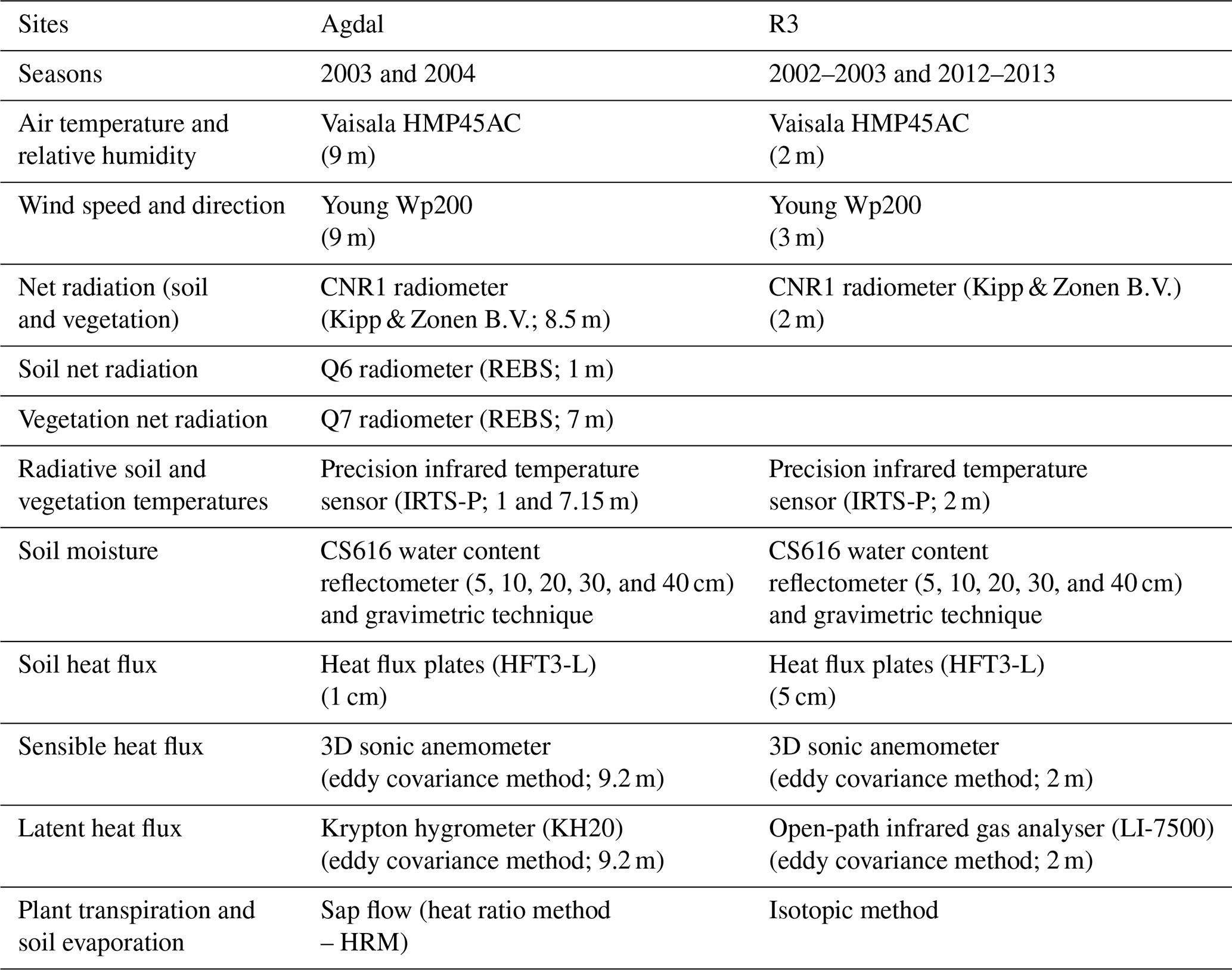
Both sites were equipped with a set of standard meteorological instruments to measure air temperature and humidity, wind speed and direction, and rainfall. Net radiation and its components were measured above the vegetation using two CNR1 radiometers (Kipp & Zonen B.V., Delft, the Netherlands). At the Agdal site, which is an open orchard, CNR1 was placed at 8.5 m height to embrace vegetation and soil radiances by ensuring that the field of view was representative of their respective cover fractions. In addition, two Q7 radiometers were used to separately measure the soil and vegetation net radiations; one was installed over bare soil at 1m and the other over olive trees at 7 m. At the same site, soil and vegetation temperatures were measured using two infrared thermometers (IRTS-Ps; Campbell Scientific, Inc., Utah, USA), with a 3:1 field of view, at heights of 1 m (pointing towards the soil) and 7.15 m (pointing towards the crown of the tree), respectively. At the wheat site, only one IRTS-P installed at 2m was used to measure the composite surface temperature. Soil heat flux density was measured at different depths using soil heat flux plates (HFT3-L; Campbell Scientific, Inc., Utah, USA) at both sites. One can note that in order to have good average values at the soil surface (about 1 cm) over olive trees, three HFT3-Ls were installed at three locations, namely underneath the canopy (always shaded), in between the trees (mostly sunlit), and in an intermediate position. Also, soil moisture was measured at both sites using time domain reflectometer probes (CS616; Campbell Scientific, Inc., Utah, USA) installed at different depths. Soil samples were also taken at both sites in order to calibrate the CS616 measurements using the gravimetric technique. All meteorological measurements were sampled at 1 Hz and 30 min averages were stored.
Finally, sensible and latent heat fluxes were measured using an eddy covariance method which consisted of a 3D sonic anemometer and krypton hygrometer (KH20; Campbell Scientific, Inc., Utah, USA) or an open-path infrared gas analyser (LI-7500; LI-COR Biosciences GmbH, Bad Homburg, Germany) that measures the fluctuations of the three components of wind speed, air temperature, and water vapour. Measurements were taken at a high frequency (20 Hz) and stored on a CR5000 data logger using a PCMCIA card (Campbell Scientific, Inc., Utah, USA). These measurements were collected and processed by an eddy covariance software (ECpack) in order to derive sensible and latent heat fluxes by including all corrections reported in Hoedjes et al. (2007, 2008), Ezzahar et al. (2007b, 2009), and Ezzahar and Chehbouni (2009). For more information, Table 1 summarises the different meteorological and micrometeorological instruments used in this study and their locations.
Table 1Overview of the different micrometeorological instruments used over the two sites.
Imbalance in the closure of the energy balance with the eddy covariance system is a good measure of the quality of the convective fluxes data. To this end, the sum of the latent heat (LE) and sensible (H) heat fluxes derived from the eddy covariance (EC) system was compared to the available energy – net radiation (Rn) minus soil heat flux (G) – at both sites. For Agdal, the closure is very good, with absolute values of average closure of about 8 % and 9 % of available energy during the 2003 and 2004 seasons, respectively (Hoedjes et al., 2008). For the R3 site, the absolute values of average closure were about 23 % and 17 % for the 2002–2003 and 2012–2013 seasons, respectively. This is considered as acceptable with regards to the literature (Twine et al., 2000).
Evapotranspiration partition
In addition to the EC observations, two techniques were used to separately measure the plant transpiration and the soil evaporation.
-
Isotopes observations: the stable isotopes tracer technique was applied for the R3 site. This technique measures the isotopic compositions of oxygen (δ18O) and hydrogen (δ2H) of water fluxes from the soil water and foliage and quantifies the rate of the plant transpiration and soil evapotranspiration to the total evapotranspiration (ET). The sampling of soil, atmospheric and vegetation water samples was made during 2 d (day of year – DOY), namely DOY 101 and DOY 102 of the growing season during 2012–2013, and the samples were analysed for their stable isotopic compositions of δ18O and δ2H. It should be noted that the sampling was made during the development stage with a cover fraction larger than 0.8. Also, the soil was very dry, with a soil moisture of about 0.12 m3 m−3, because the experiment was conducted before an irrigation event which was applied on DOY 104. Atmospheric water vapour was sampled from four heights (0 cm, 85 cm, 2 m, and 3 m), between 10:00 and 16:00 local time (LT), with a frequency of 1 h on each sampling day. In addition, the samples of soil and vegetation were collected between approximately 13:00 and 14:00 LT. Afterwards, these samples were used to calculate δ2H of the soil, vegetation, and atmosphere in order to estimate the ET partition based on the Keeling plot approach and then to compare it with the modelled soil evaporation and plant transpiration. More details about the description of the principles and techniques of the observations can be found in Aouade et al. (2016).
-
Sap flow observations: the heat ratio method (HRM) was applied for the Agdal site to measure xylem sap flux of eight olive trees using heat pulse sensors. The period of measurement was between 9 May (DOY 130) and 28 September (DOY 272) during 2004. This period was characterised by a hot climate, with very high surface temperatures, and thus presented a perfect period for studying the ET partition over such surfaces. In brief, this method uses temperature probes which were inserted into the active xylem at equal distances upstream and downstream from the heat source. This method was chosen due to its high precision at low sap velocities and its robust estimation of transpiration of olive trees (Fernández et al., 2001). The heat pulse sensors were inserted into large single and multistemmed trees located in the vicinity of the EC tower. The transpiration at the field scale (in mm d−1) was obtained by scaling the measured volumetric sap flow (L d−1), based on a survey of the average ground area of each tree (45 m2). This is obtained by plotting the measured total evapotranspiration against the sap flow observations under dry conditions, leading to lower surface soil moisture when the soil evaporation is considered negligible (Williams et al., 2004; Er-Raki et al., 2010). This equation is then generalised for wet conditions of sap flow observations for deriving the stand level plant transpiration. Finally, based on the EC observations, the single tree transpiration obtained was extrapolated to the EC footprint scale which is representative of the whole field (Er-Raki et al., 2010). Consequently, this can generate a significant error in estimating stand level plant transpiration as previously reported in several studies (Fernández et al., 2001; Williams et al., 2004; Oishi et al., 2008; Er-Raki et al., 2010).
Vegetation characteristics and irrigation inputs
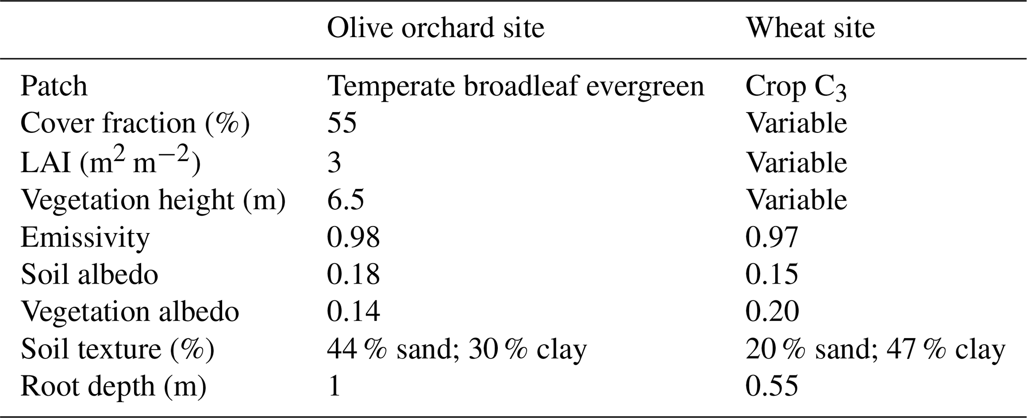
For the olive site, the mean vegetation fraction cover (Fc) and the leaf area index (LAI) obtained from one campaign of hemispherical canopy photographs (using a Nikon Coolpix 950 digital camera fitted with a fisheye lens converter (FC-E8); field of view – 183∘) are equal to 55 % and 3 m2 m−2, respectively. For the wheat site, Fc and LAI together with vegetation height hc were measured about every 15 d using the same instrument. The irrigation dates and amounts were also gathered by dedicated surveys. The time series of the LAI and reference evapotranspiration ET0 are provided in the Supplement (Fig. S1).
2.2 The ISBA-A-gs model description and implementation
2.2.1 Model description
ISBA is a land surface model used to simulate the heat, mass, momentum, and carbon exchanges between the continental surfaces (including vegetation and snow) and the atmosphere. It also prognoses temperature and moisture vertical profiles in the soil. The first developed version of the ISBA model, named hereafter as the standard version, was based on a simple soil–vegetation composite scheme to compute the surface energy budget and was developed by Noilhan and Planton (1989) and Noilhan and Mahfouf (1996). It is implemented within the open-access SURFace EXternalisée (SURFEX) platform version 8.1 developed by Centre National de Recherches Météorologiques (CNRM) at Météo-France (Masson et al., 2013). In this study, a multilayer soil diffusion scheme (Decharme et al., 2011) is used to simulate the soil water and heat transfers instead of the initial force–restore formulation (Deardorff, 1977). The soil is vertically discretised by default into 14 soil layers up to a 12 m depth to ensure a realistic description of the soil temperature profile (Decharme et al., 2013). The moisture and temperature of each layer are then computed according to their textural and hydrological characteristics. The latter (hydraulic conductivity and soil matrix potential) are derived from the Brooks and Corey (1966) parameterisation following Decharme et al. (2013). The stomatal conductance and the photosynthesis are computed using the CO2-responsive parameterisation named A-gs (Calvet et al., 1998, 2004). The model includes two plant responses to soil water stress functions depending on the plant strategy with regards to drought (Calvet, 2000; Calvet et al., 2004). The non-interactive vegetation option is chosen, meaning that vegetation characteristics (LAI, height, and fraction cover) are prescribed from in situ measurements with a 10 d time step. The multilayer solar radiation transfer scheme (Carrer et al., 2013), which considers sunlit and shaded leaves, is also activated. The root density profile is a combination of a homogeneous profile and of the Jackson et al. (1996) exponential profile (Garrigues et al., 2018). Full expressions of the aerodynamic resistances are given in Noilhan and Mahfouf (1996).
Compared to the standard version of ISBA-Ags, ISBA–MEB, for multiple energy balance, solves up to three separated energy budgets for the soil and the snowpack following Choudhury and Monteith (1988). In this study, a double source arising from the soil and from the vegetation is used. For extended details about the different hypothesis used in MEB version and its full mathematical formulas and related numerical resolution methods, one is referred to Boone et al. (2017). The main governing equations of both versions of the model are given in Appendix A.
2.2.2 Model implementation
Input parameters and data
ISBA within SURFEX is intended to be implemented using the patch approach in which each grid point can include up to 19 patches representing 16 different plant functional types, bare soil, rock, and permanent snow. Within the SURFEX platform, input parameters and variables are usually derived from the ECOCLIMAP II database (Faroux et al., 2013). In this study, ECOCLIMAP II is bypassed by using in situ measurements for most of vegetation characteristics and albedo. For the wheat site, 10 d vegetation characteristics (LAI, hc, and Fc) were derived from in situ measurements based on a linear interpolation. Annual constant values were used for the olive orchard. The roughness length for heat and momentum exchanges (Z0 m and Z0 h, respectively) is derived from hc following Garratt (1992), namely and . The emissivity and the total albedo are obtained as a linear combination of the soil and vegetation characteristics weighted by the fraction cover. The total albedo derived from the two components of the short-wave net radiation measured by the net radiometer (CNR1) instruments is used to calibrate the albedos of vegetation and soil for the whole study field. The two component albedos remain constant for the whole set of simulations, while the total albedo evolves through the vegetation cover fraction changes. The input data for the two sites are summarised in Table 2. Soil hydraulic properties were computed from the Clapp and Hornberger (1978) and the Cosby et al. (1984) pedotransfer functions. The resulting parameters were quite similar, namely Wwilt=0.25 and Wfc=0.34 for Clapp and Hornberger (1978) and Wwilt=0.26 and Wfc=0.33 for Cosby et al. (1984) Nevertheless, values based on the calibration of soil moisture time series were quite different (Wwilt=0.18 and Wfc=0.41). Beyond the inherent uncertainties of the pedotransfer functions, this may be mostly explained by the lack of representativity of the soil sampling. Calibrated Wwilt and Wfc were imposed.
Table 2Input parameter and variables of the ISBA model derived from in situ measurements.
Model configurations
Three structural representations of the canopy are compared in this work: (1) the composite energy balance of the standard version, named ISBA-1P for the single patch version; (2) the uncoupled version, named ISBA-2P for two patches, where the canopy and the soil patches are situated side by side, resolves two energy balance equations for both patches without any interactions concerning the turbulent heat exchanges (likewise, the soil water dynamic is predicted on two uncoupled soil columns); and (3) the coupled two-layer approach of the new MEB version, ISBA–MEB, where the canopy layer is located above the soil component and the energy budgets of both layers are implicitly coupled with each other (Boone et al., 2017). Note that the ISBA-2P configuration is implemented at the olive orchard only as there is no reason to represent the homogeneous canopy of wheat crops with two patches located side by side. Figure 2 displays the schematic representation of the three configurations of the model.

Figure 2Schematic description of the three configurations of ISBA model: (a) the single-source configuration (ISBA-1P), (b) the layer configuration (ISBA–MEB), and (c) the patch configuration (ISBA-2P).
2.3 Sensitivity analysis and parameter calibration
2.3.1 Sensitivity analysis and calibration methods
Analysing the sensitivity of the parameters one by one is not satisfactory because of the parameter interactions and non-linearities in the model equations and in the underlying processes (Pianosi et al., 2014). For this reason, the multi-objective generalised sensitivity analysis (MOGSA; Goldberg, 1989; Demarty et al., 2005) is chosen in this study. The MOGSA methodology uses a Monte Carlo sampling of the search space. To represent the uncertainty of parameter estimates, an ensemble of N parameter set is drawn stochastically within a range of physically realistic values using an uniform distribution. A threshold on the targeted objective functions is then used to partition the ensemble into acceptable and unacceptable regions. The trade-off between the targeted objectives is sought using a Pareto ranking scheme. The cumulative distribution of the parameter's value is compared to the normal distribution through the statistical Kolmogorov–Smirnorff (KS) test that relates this maximal distance to a probability value. The application of thresholds to this probability value permits the quantification of the degree of parameter sensitivity. An ensemble of 20 000 simulations for Agdal and 40 000 for the R3 sites were computed. The size of the simulations is related to the size of the studied period. Based on the recommendations of Demarty (2001), it is assumed that the size of the samples was large enough to obtain robust results. No account was taken of possible covariation between the parameter values in these prior choices of parameter sets because such covariation is generally difficult to assess. Several objective functions were explored, namely latent heat (LE) and transpiration Tr, sensible heat H and Tr, and LE∕H. As similar sensitive parameters were highlighted, the chosen objective functions in this work were the convective fluxes H and LE. The MOGSA algorithm is also used to retrieve the parameter set providing the best trade-off of objective functions (Demarty et al., 2005). This parameter set will hereafter be called “optimal”. The ISBA model was thus calibrated by taking the best parameter set among the 20 000 and the 40 000 tested in the multi-objective sense. Finally, the validation step was carried out over the 2004 and 2013 seasons for Agdal and R3, respectively.
2.3.2 Sensitive parameters selection
For our sensitivity study, a total of 16 parameters (φv and are for MEB only) were identified based on previous knowledge of the model and the rich literature based on the use of ISBA-A-gs and ISBA–MEB (Calvet et al., 2008; Calvet and Soussana, 2001, Boone et al., 1999, 2009, 2017; Napoly et al., 2017). The list of parameters and their ranges of variation are reported in Table 3. The land cover database obtained from ECOCLIMAP (Masson et al., 2003) and ECOCLIMAP-II (Faroux et al., 2013) were used to prescribe the range of variations of the input parameters. The same sensitivity analysis and calibration study was conducted for the standard single-source version and the MEB version of ISBA. The sensitivity analysis was carried out for the whole 2003 wheat season for the R3 site and between 1 June and 30 August (2003) at the olive orchard (Agdal site) in order to limit the computing time.
Table 3List of parameters used for sensitivity analysis and their considered ranges.
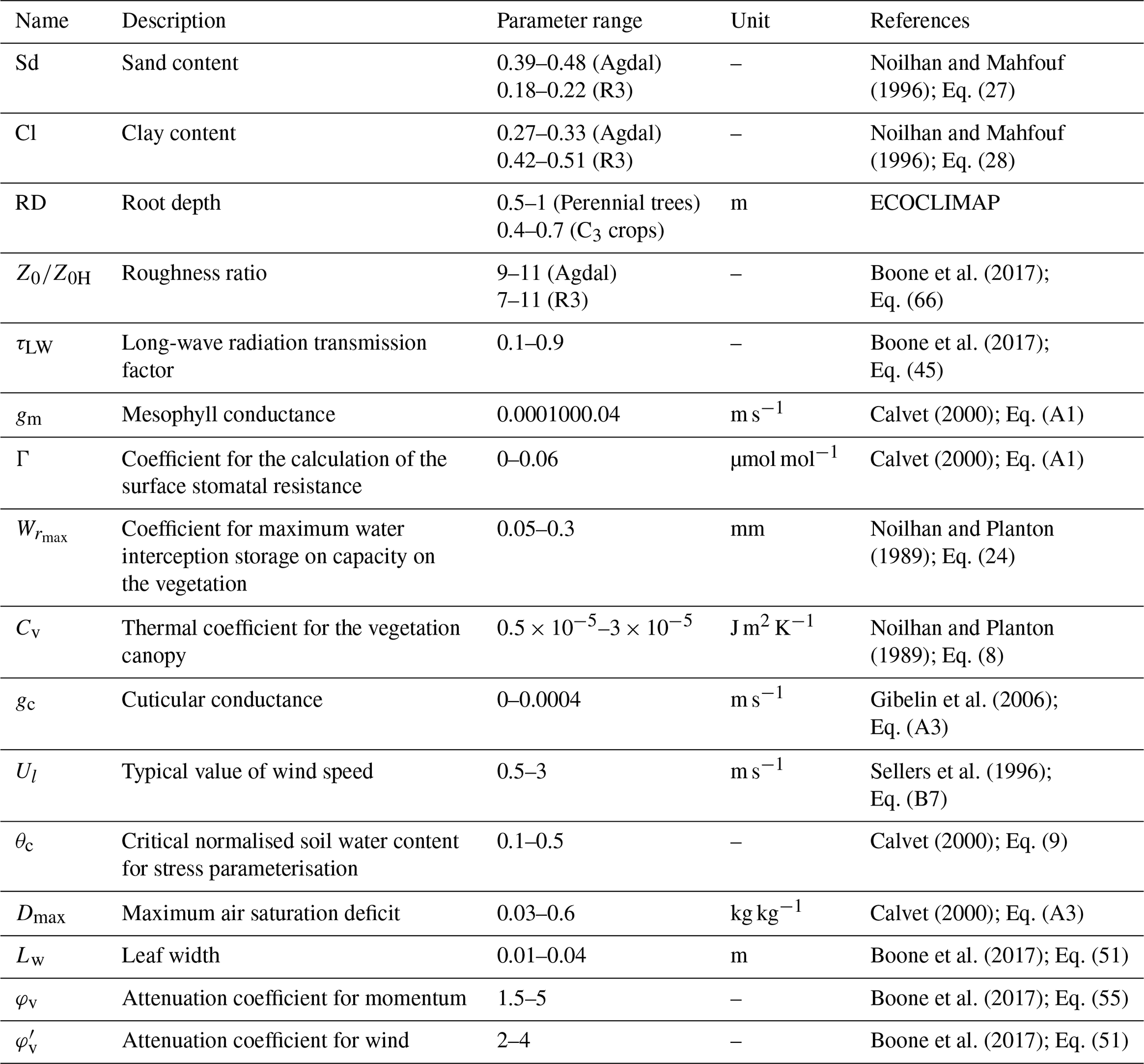
The parameters list includes (1) some parameters well known to be highly sensitive, such as the soil texture, the root depth, and the ratio of roughness lengths Z0∕Z0H; (2) some parameters of the A-gs module containing the mesophyllian conductance in unstressed conditions gm, the maximum air saturation deficit Dmax, the cuticular conductance gc, and the critical normalised soil water content for stress parameterisation θc (Calvet et al., 2004; Calvet, 2000; Rivalland et al., 2005); and (3) the new parameters which were introduced in ISBA–MEB, such as the long-wave radiation transmission factor, which determines the partition of this radiation between vegetation and soil (Boone et al., 2017) and the attenuation coefficient for momentum and for wind that prescribe changes based on canopy heights, turbulent transfer coefficients, and wind speed (Boone et al., 2017; Choudhury and Monteith, 1988). The values of these two parameters are, in the current version of ISBA, constant and independent of the type of canopy (φv=2 and ), while Choudhury and Montheith (1988) have shown that this model is sensitive to the variation of those two parameters and, in particular, to the temperature of the ground surface, which depends, among other things, on the aerodynamic resistance between the source of movement at the vegetation level and the soil surface. Likewise, the aerodynamic resistance between the vegetation and the air at the vegetation level is related to and to the Leaf width Lw (Choudhury and Monteith, 1988).
All parameters are common between the two versions except φv, , and Lw which concern the MEB version only.
3.1 Sensitivity analysis and calibration
Only the results of ISBA–MEB are presented here as quite similar list of sensitive parameters is obtained with the standard version of ISBA. The simulations are partitioned into two groups, namely acceptable and unacceptable. Demarty et al. (2005) suggested that 7 % to 10 % of members should comprise the acceptable set. In this context, 1720 acceptable simulations for the Agdal site (8.6 %) and 3600 for the wheat site (9.0 %) are retained. Figure 3 displays the results of the sensitivity analysis obtained for both sites. The horizontal broken lines indicate the transition levels between low, medium, and high sensitivity (Bastidas et al., 1999). Table 4 reports the optimal values of the highly sensitive parameters for at least one of the objective functions.
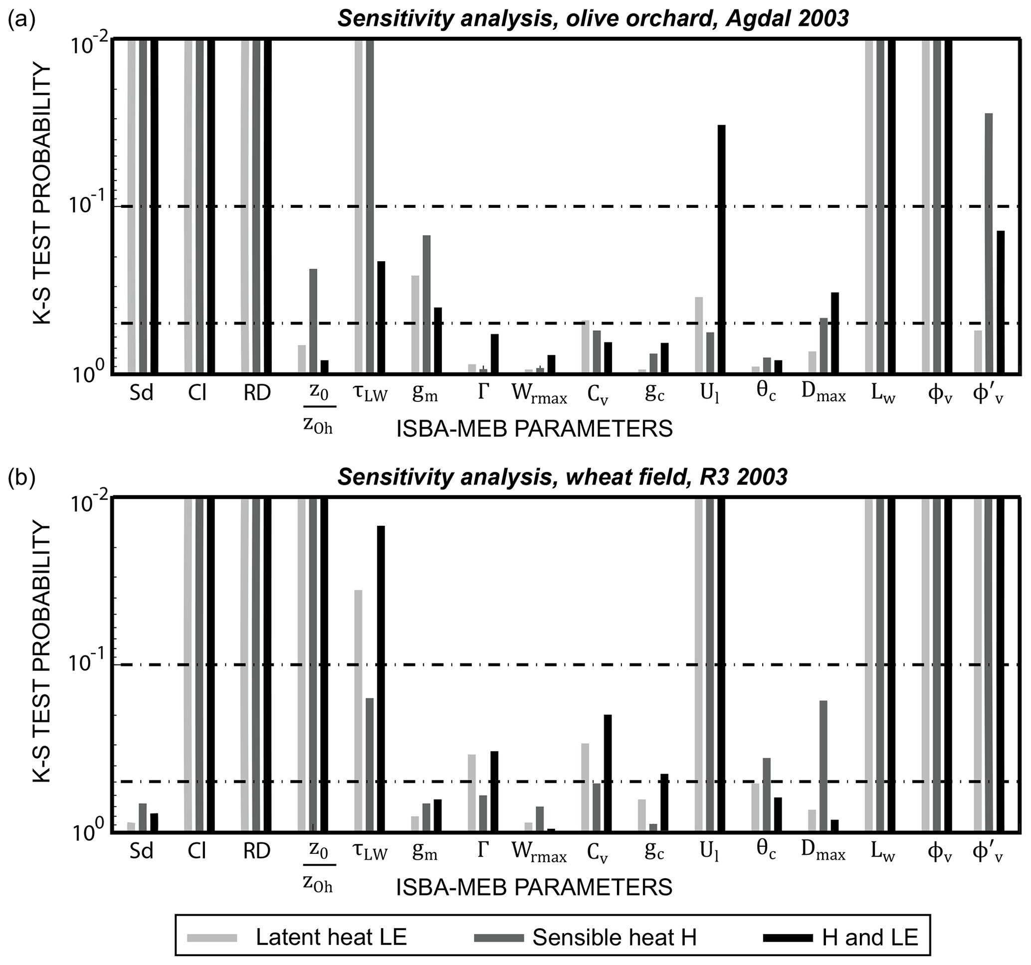
Table 4Default values from the literature or ECOCLIMAP-II database and optimal values (see text) of the highly sensitive parameters for one of the objective functions.
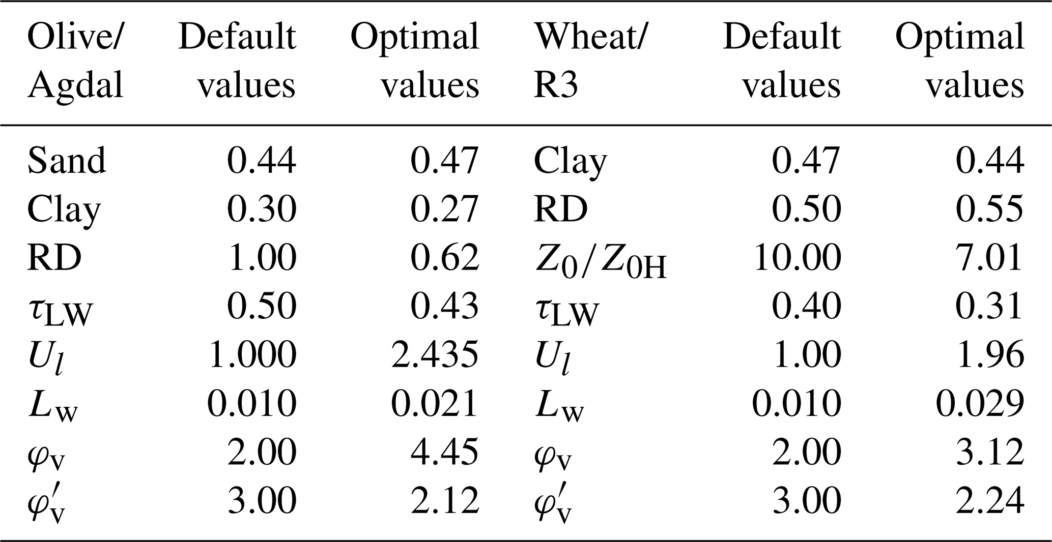
The high sensitivity of some parameters was anticipated such as (1) the soil-texture-related parameters (fraction of sand and/or clay) that strongly impact the hydrodynamic characteristics of the soil and, ultimately, the fluxes (Garrigues et al., 2015); (2) the root depth that has a major role in the extraction of available water in the root zone (Calvet et al., 2008); (3) the ratio of roughness lengths Z0∕Z0H, which impact the calculation of the aerodynamic resistance. Those parameters which highly affect the model behaviour are usually estimated through in situ measurements or for a large-scale application from global database. In both cases, their values are uncertain, even at the station scale, as their spatial variability remains significant, including the soil texture along the vertical profile. Five other sensitive parameters are also common to both sites, particularly the long-wave transmission factor τlw introduced in the new radiative transfer scheme and the parameters introduced in the ISBA–MEB version Lw, φv, , and Ul. Concerning the attenuation coefficient of the movement φv, Choudhury and Montheith (1988) had already shown the strong sensitivity of the model to this parameter, especially for dry soils encountered in our study sites.
Concerning the Agdal site, results showed 11 sensitive parameters, 8 parameters with high sensitivity, and 3 with medium sensitivity (Fig. 3a) when at least one of the objective functions are considered. The chosen period was characterised by a gradual drying of the soil with a water stress detected on DOY 190 (Ezzahar et al., 2007a). The plant transpiration thus represented the main component of the evapotranspiration. Within this context, the identified sensitivity of parameters directly impacting the stomatal regulation (gm, Dmax) and the availability of water in the soil (Sand, Clay and RD) is consistent. Regarding the moderate fraction cover (Fc=0.55) and the flooding technique applied for irrigation, soil evaporation also tightly related to soil texture may not be negligible on the site. Interestingly enough, the obtained optimal values of 0.47 for sand and 0.27 for clay (Table 4) were very close to the in situ measurements. The root depth (RD) also strongly influences convective fluxes. An optimal value of 0.62 m was found, while the literature and ECOCLIMAP propose a deeper rooting depth up to 1.5 m for perennial trees. Nevertheless, it is well known that roots develop in the upper wet layer of the soil when irrigation is applied (Fernandez et al., 1990), while deeper development can be observed in case of water supply problems only (Maillard, 1975). Additionally, the soil in our site below 1 m is very compact and contains rocks, which limit the development of the pivoting roots.
For the wheat site, the sensitivity analysis revealed 13 sensitive parameters, as 8 of them have a high sensitivity and 5 of them have a medium sensitivity (Fig. 3b). As for the Agdal site, specific parameters are related to the soil (like Cl) and others are related to the crop (RD, Lw, and τlw). In contrast to Agdal, the two fluxes, LE and H, also showed a strong sensitivity to the Z0∕Z0H parameter. In the standard version of ISBA-A-gs, this ratio is equal to 10 according to Braud et al. (1995) and Giordani et al. (1996), but at the station scale, several studies have shown that this ratio could range from 1 to 100 (Napoly et al., 2017). The optimal value for the wheat site was 7.00. The obtained optimal lower value increases the amplitude of H and reduces that of the surface temperature. This is consistent with similar findings of Béziat et al. (2013) for a wheat site located in the southwest of France. The literature and ECOCLIMAP propose values of root depths of about 0.50 m for our type of crop (crop C3). In our case, a slightly higher value of 0.55 m appeared optimal for latent heat fluxes and also for transpiration when compared to the isotopic measurements (see comments below and Table 4). This is an acceptable value for irrigated wheat in the region (Duchemin et al., 2006; Er-Raki et al., 2007). Due to the limited number of irrigations at this site, the plants tend to extend roots to deeper layers to extract water. The slightly lower value of the clay content (0.44) compared to the in situ measurement (0.47) adjustment is also consistent with limiting water retention, and it favours water availability in the deepest layers. Regarding the evapotranspiration flux, in the case of a dry soil, the only possible solution for reproducing the experimental data is to increase the transpiration of the crop. Indeed, the strong sensitivity of the two parameters φv and seems to be consistent (Choudhury and Idso, 1985). In addition, the optimal value for φv () is higher (lower) than the literature (Table 4).
As a conclusion, because the optimal values of the sensitive parameters are significantly different to the values in the literature, studies at the local scale should be duplicated to determine specific parameter values for different ecosystems and agrosystems in the view of large-scale applications.
3.2 Composite energy budget
3.2.1 Latent heat flux
Figure 4 displays the daily time series of latent heat fluxes using the three configurations of the ISBA model for both sites. The irrigation and rainfall events are also superimposed. Please note that, hereafter, daily values refer to the average of diurnal values between 09:00 and 17:00 LT (local time). The same figure, but for the sensible heat flux, is provided in Fig. S2. Statistical metrics for the four components of the energy budget are reported in Table 5. The seasonal dynamic of LE is properly reproduced by the model for both sites, whatever the configuration. ISBA-2P and ISBA–MEB definitely outperformed the ISBA-1P version, on average, at the olive orchard for both seasons, with RMSE values below 52.2 W m−2, while for ISBA-1P, RMSEs can reach up to 107.1 W m−2. This corresponds to the average errors of 19 % and 16 % for MEB in 2003 and 2004, respectively; 28 % and 21 % for ISBA-2P while average error is about 42 % for ISBA-1P during both years. In contrast, at the wheat site, the ISBA-1P version is much closer to ISBA–MEB, with differences in RMSEs at around 10 W m−2. The average errors are also close, with 23 % versus 21 % for MEB and ISBA-1P in 2003 and 26 % versus 28 % in 2013. This means that:
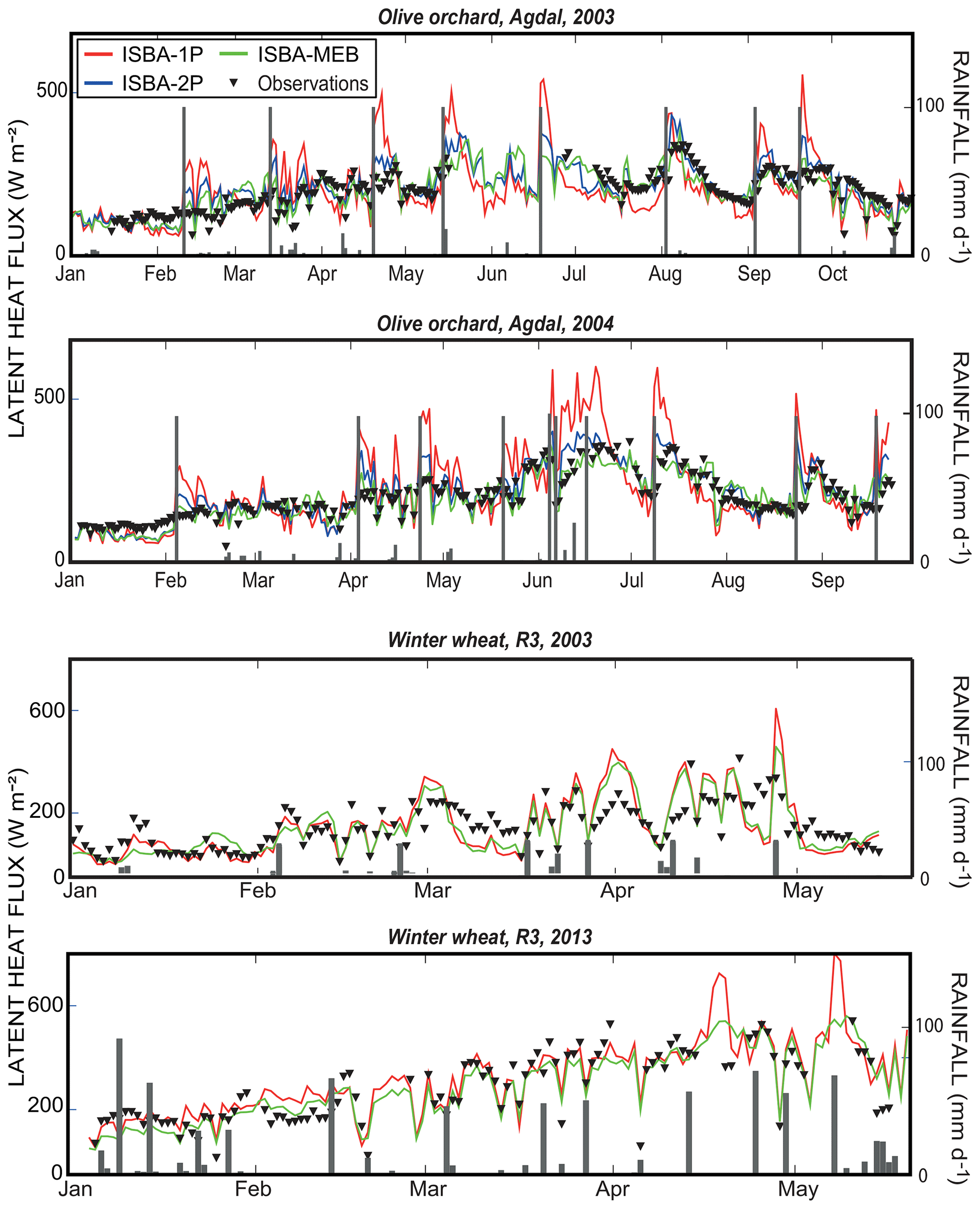
Figure 4Time series of the daily average simulated and measured latent heat flux (LE) for the Agdal site (2003 and 2004 seasons) and for the R3 site (2003 and 2013 seasons).
Table 5Comparison between observations and ISBA for the components of the energy balance through the root mean square error (RMSE), correlation coefficient (r), and bias (Bias). The calibration period is 2003 for both sites, while validation is 2004 for Agdal and 2013 for R3.
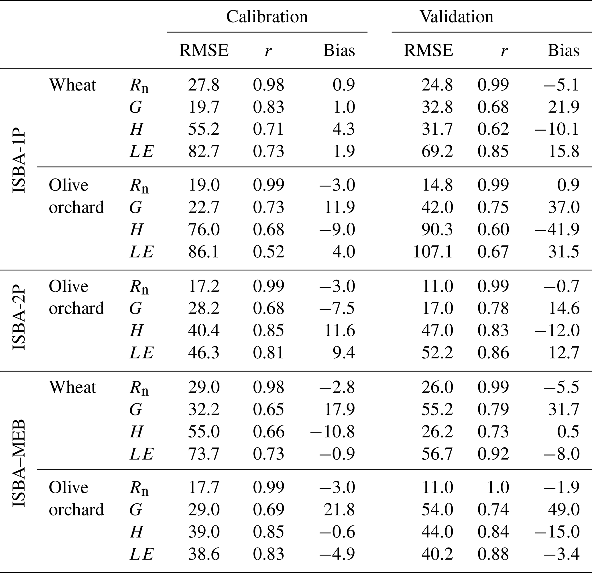
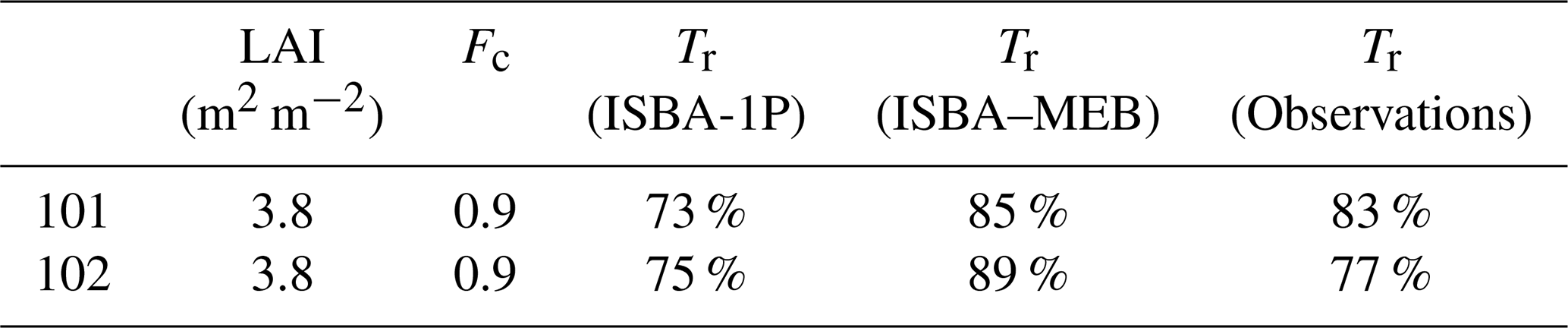
Table 6Percentages of transpiration simulated by the three configurations of the ISBA model and measured with the isotopic method for the 2013 season at the R3 site. The corresponding LAI and Fc are also provided.
-
The dual-source configurations are better suited for predicting composite LE for row crops of a moderate fraction. This result is in line with Napoly et al. (2017; Fig. 15b), ISBA-1P and ISBA–MEB differences (biggest improvements for MEB) are largest for LAI values in the range from 3 to 4 m2 m−2 corresponding to moderate Fc, which corresponds to the LAI for the olive grove in this study. This arises mainly because the differences between the surface and the vegetation (temperatures, fluxes, etc.) are most contrasted for sparse vegetation cover. In contrast, when Fc tends to 1, ISBA-1P resembles a complete vegetation surface and ISBA–MEB and ISBA-1P should converge.
-
In contrast, as expected, a simple composite energy budget can cope with the homogeneity of the wheat canopy – at least to predict LE. Generally speaking, the difference between ISBA-1P and ISBA–MEB in terms of surface temperatures, fluxes, etc. is expected to decrease as the cover decreases in height; the results converge as the surface becomes devoid of vegetation. So, results tend to be closer for grasses and annuals just like wheat and trees. This is because the main differences arise owing to the difference in the within-canopy turbulence treatment; i.e. both versions use the same functions based on the Monin–Obukhov Similarity Theory (MOST) above the momentum sink point (Z0 for ISBA-1Pand Z0+d for ISBA–MEB, where d is the displacement height) meaning that as the d→0, the models converge to a certain extent. Likewise, when Fc tends to 1, ISBA-1P resembles a completely vegetated surface and ISBA–MEB and ISBA-1P converge. The added value of a double energy budget should thus be evident from the emergence until the full cover when vegetation is sparse. The surface can be considered homogeneous out of this period, by either considering bare soil at the start of the season or fully covering vegetation at the end of the season. In contrast, from the emergence to the full cover, the cover sparsity may lead to a strong difference between soil and vegetation temperatures, and some level of coupling between both energy sources, but this period is short for wheat. It covers less than 1 month around march at ±10 d.
-
The slightly better results obtained with ISBA–MEB than with ISBA-2P at the olive orchard demonstrates that the soil and the vegetation heat sources are coupled to some extent. This is probably because the bare soil area between the tree rows (the interrow is about 8 m) is not sufficiently large to consider that soil and vegetation heat sources do not interact with each other by locating the two sources side by side.
Previous studies have already demonstrated the limits of single-source models for predicting surface fluxes over sparse vegetation. Jiménez et al. (2011) have evaluated four single-source models (namely, Mosaic, Noah, Community Land Model – CLM, and Variable Infiltration Capacity – VIC) at the global scale and they showed their limitations for producing latent and sensible heat fluxes over tall and sparse vegetation such as forest canopies. Likewise, Blyth et al. (1999) estimated the surface fluxes more accurately over the Savannah in the Sahel with the dual-source version of the MOSES model compared to the original single-source version. Our results with the new ISBA–MEB version, implemented within the SURFEX platform, are consistent with these previous findings.
Another interesting feature is the observed departure between model predictions and observations around irrigation events. Nevertheless, the different configurations of the model strongly differ during these specific periods, particularly at the olive site. In line with the observations, the three configurations show a strong shift of the available energy from sensible to latent heat when irrigation occurs (see also sensible heat flux time series; Fig. S2) but, while this shift is moderate and in overall agreement with the observations for the dual-source configurations, it is strongly emphasised by ISBA-1P. For instance, LE predictions reached a maximum of about 550 W m−2 in mid-June for both seasons of 2003 and 2004 when observations remained below 400 W m−2. To a lesser extent, this trend to unreasonable shifting also occurred for the ISBA-2P, especially when the available energy is very high (during the summer months of the 2003 season). The reverse behaviour is obviously observed for H (Fig. S2); after each irrigation event, the simulated sensible heat by ISBA-1P dropped considerably due to the drastic decline in simulated surface temperature of this version. In addition to the model deficiencies at the time of irrigation as already highlighted, part of the discrepancies between simulations and observations can be related to the eddy covariance measurements because of the associated strong heterogeneity within the footprint during an irrigation event.
In contrast, on the wheat site, the dynamics of the latent heat flux is smoother than at the olive site in 2013 and, to a lesser extent, in 2003, particularly because of a persistent cloud cover during the first two weeks of March (see the drastic drop of ET0; Fig. S1). The year 2003 is also characterised by lower LE values, mainly because several successive drought years at the beginning of the 2000s caused a drop in dam levels and limited the water availability for irrigation. Indeed, the total cumulated rainfall and irrigation was 351 mm for the 2002–2003 season, while it reached about 770 mm for 2012–2013. In contrast to the olive site, the two configurations of the model are able to reproduce the overall seasonal dynamic of LE for these 2 contrasting years. The only exception is around the late season irrigation events in April and May 2013, during which ISBA-1P showed the same trend of strongly emphasising the energy shift, as already highlighted for the olive site.
As a conclusion, while the dual-source configurations outperformed the single-source version of the model for the complex and sparse olive canopy, a composite single energy budget is able to reproduce the seasonal dynamic of LE for the homogenous wheat cover. At this level of sparsity for the olive orchard, the coupling between soil and vegetation heat source is moderate as both the uncoupled patch and the coupled-layer configurations provided close statistical metrics. For the olive site, a significant drawback of ISBA-1P and, to a lesser extent, ISBA-2P is highlighted during the strong transient regime associated with the irrigation events.
3.2.2 Other components of the energy budget
The performance of the different configurations to simulate the other components of the energy budget Rn, H, and G was investigated using a Taylor diagram (Fig. 5). This presentation graphically summarises the comparison between the model and the observations based on the root mean square difference, the correlation coefficient r, and the standard deviations (Taylor, 2001). Statistical metrics are reported in Table 5.
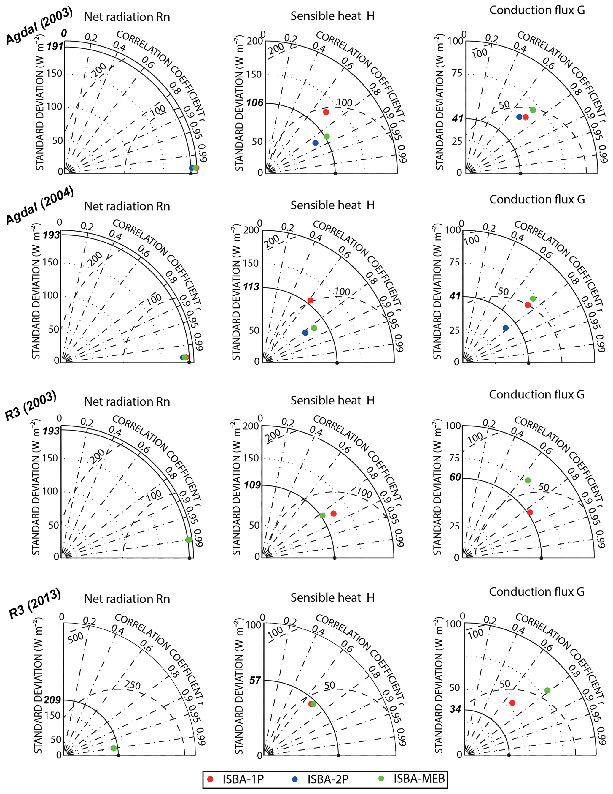
Figure 5Taylor diagrams for the net radiation Rn, the sensible heat flux H and the ground heat flux for Agdal (2003 and 2004 seasons) and R3 sites (2003 and 2013 seasons). ISBA-1P is in red, ISBA-2P is in blue, ISBA–MEB is in green, and observations are indicated using a black dot.
The net radiation is almost perfectly simulated by the three configurations, with slight differences related to the budget in the long wave. Values of the albedo are identical for the three configurations and have been calibrated on the short-wave components of Rn measured by CNR1. For both sites, the correlation coefficient r is close to 1.0, and the RMSE is lower than 25.0 W m−2. These good performances are in agreement with results reported in the literature. Indeed, several studies showed that the estimation of Rn by SVAT models is good on several types of canopy (Napoly et al., 2017; Boulet et al., 2015; Ezzahar et al., 2007a, 2009). The most important differences are encountered at the Agdal site and can be explained by the slight overestimation (not shown) of the infrared radiation (LWup) by ISBA-2P for both seasons (Bias = 13.7 and 12.7 W m−2 for the 2003 and 2004 seasons, respectively). For this configuration, the soil of the soil patch directly exposed to the solar radiation becomes very hot and dissipates much less energy from soil conduction compared to the other two configurations. This is due to a compensation between the soil and the vegetation patches, as explained below.
For the sensible heat fluxes (Fig. S2), the dual-source configurations, ISBA-2P and ISBA–MEB, also outperformed the single-source version, ISBA-1P, for sensible heat flux predictions at the olive orchard. In contrast, the two tested configurations are much closer for the wheat site, with RMSEs of 55.2 and 55.0 W m−2 in 2003 for ISBA-1P and ISBA–MEB, respectively. The temporal dynamics are also greatly improved since the correlation coefficients (r) are above 0.8 for the dual-source configurations for the two seasons at the olive orchard site, whereas they are only 0.7 and 0.6 for the single-source approach. Here again, it is the shifting between sensible and latent heat fluxes during the irrigation events and during the drying period that leads to the differences between single- and dual-source configurations. For the wheat site, the behaviours are very similar for the two configurations, although the MEB version presents the best performances.
Due to the complexity of the canopy surface and the spatial variability of the hydric and thermal conditions, particularly because of the effect of shade, the ground heat flux is the most difficult component of the energy budget – both to simulate and to measure. The heat plate fluxes used on both studied sites have a very low representativeness, which does not exceed a few tens of centimetres, whereas the illumination can be very variable under a relatively open canopy, such as olive, or over wheat at the beginning of the season. Therefore, the obtained results should be interpreted with caution. The highlighted improvement on the turbulent fluxes using MEB, compared to the two other configurations, is not so clear for the conduction fluxes. It seems that MEB has a systematic tendency to dissipate too much energy from conduction (see biases in Table 5). On average, over the 2 years for the olive site, the ISBA-2P configuration has the best overall performance in predicting G. Nevertheless, by taking a closer look on the daily cycles of the ground heat flux with a distinction between the bare soil patch and the vegetation patch (see Fig. S3), it appears that the bare soil patch dissipates much more energy from conduction than ISBA–MEB, as shown by the amplitude of the daily cycles which is much stronger than the observations. In contrast, the vegetation patch (LAI = 5 and a cover fraction close to 1) dissipates less energy through conduction in favour of the convective fluxes. The average ground heat flux (derived as the sum of the two components weighted by their respective fraction cover) is in good agreement with observations, even if none of the two patches represent the observed fluxes correctly. This tends to show that the uncoupled approach is quite suitable for predicting total G at this sparse and relatively open cover but for the wrong reasons. Finally, ISBA-1P also dissipates much more energy than ISBA–MEB because the soil experiences little shade, as explained below (see Sect. 3.1.1).
3.3 Soil and vegetation components
In this section, the soil and vegetation components of the radiation budget and of the partition of evapotranspiration are analysed. Please note that only the olive orchard site was considered for the radiation budget components as the experimental design on the wheat site could not sample each component separately. For ISBA-2P, vegetation and soil refers to the component predictions of the respective patches, while for ISBA-1P the soil–vegetation composite variables are plotted.
3.3.1 Radiation budget
Figure 6a displays the time series of the soil net radiation simulated by the three configurations at the Agdal site in the 2003 season. Similar conclusions can be drawn from the data acquired in 2004. The bare soil patch is shown for the ISBA-2P configuration. The amplitude of the seasonal cycle is much stronger for the observations than for the ISBA simulations. The net radiation at the soil surface is obviously lower for ISBA–MEB because of the vegetation screening and a real partition between the two sources than for ISBA-1P and ISBA-2P (soil patch). Indeed, for ISBA-1P, there is no partition of net radiation between soil and vegetation. Stated differently, since there is only one energy budget, the soil temperature is the same as the temperature of the vegetation, and the soil experiences very little shade (in addition, it uses the same relatively large Z0 since the non-linear aggregation of Z0 for soil and vegetation tends to result in a Z0 much closer to the higher elements, the vegetation z0, than one would expect). The high energy available(Fig. 6) is used for soil evaporation at the time of irrigation (see Fig. S4), unless Fc→1. ISBA–MEB is in better agreement with observations during the winter months, while the agreement is better in summer for ISBA-2P and ISBA-1P. The strong differences may also be related to observations. Indeed, the soil net radiation was measured under the cover. When the cover is sparse, as for the olive trees, it is very difficult to screen it totally from direct incoming radiation as, during summer, with a solar zenith angle close to 0, the instrument is exposed to direct radiation. In winter, ISBA–MEB appears to be reproducing the measurements of the available energy at the ground-level well when it may be in the shade of the canopy. When the instrument is exposed to direct illumination, the ISBA-1P configuration and the bare soil patch of the ISBA-2P configuration are obviously closer to observations.
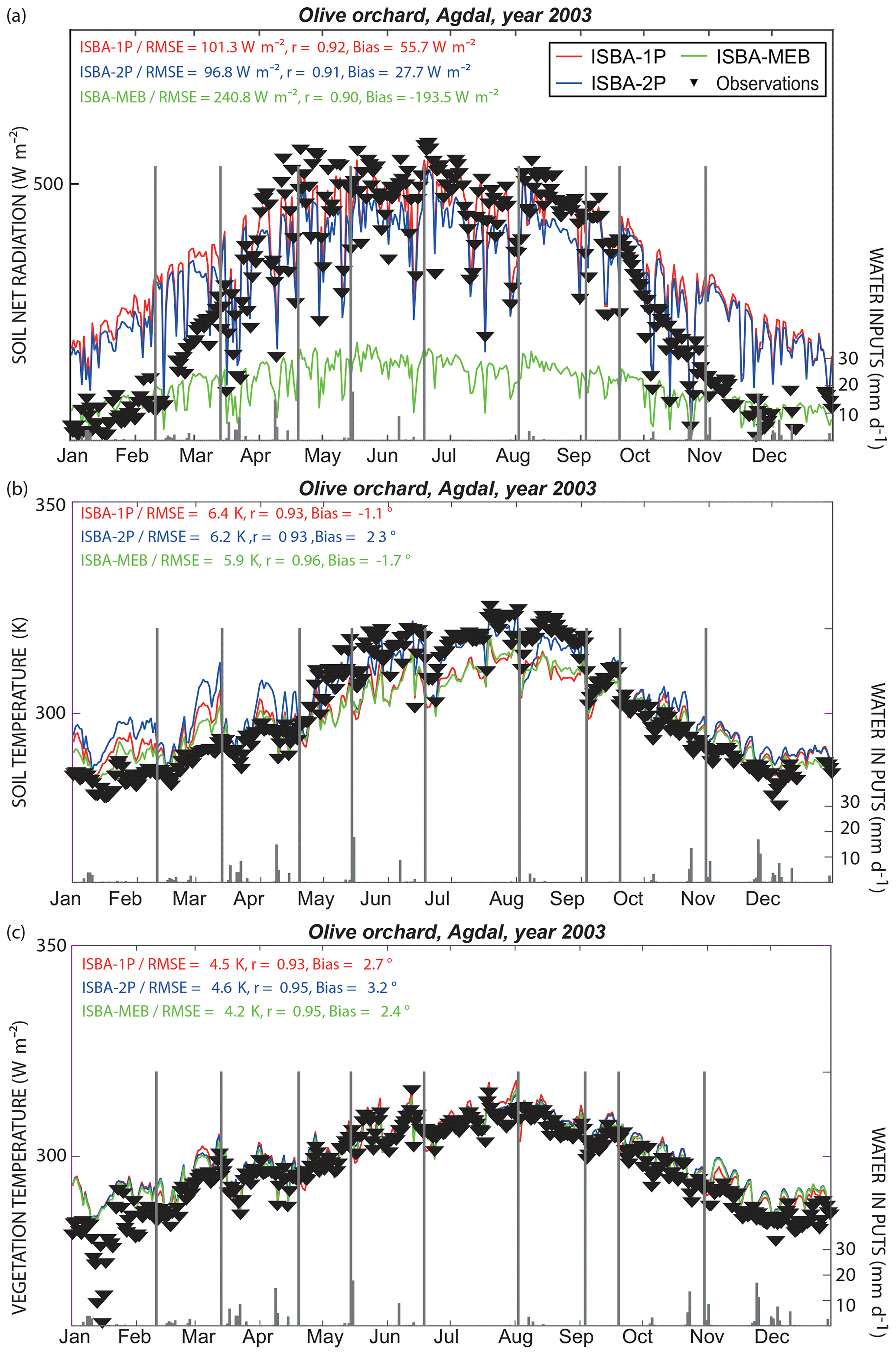
Figure 6Time series of the daily average soil net radiation (a; only the bare soil patch is shown for the ISBA-2P configuration), daily average soil temperature (b), and daily average vegetation temperature (c) simulated by the three configurations and measured at the Agdal site for the 2003 season.
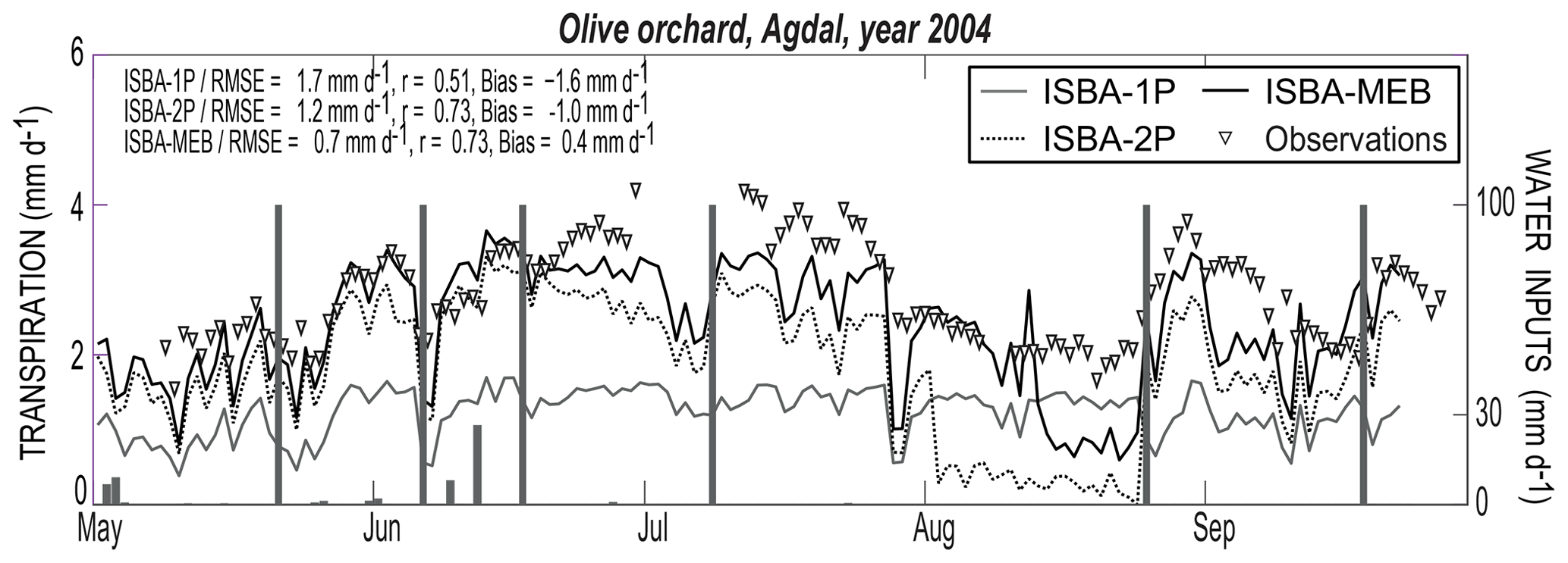
Figure 7Time series of the daily cumulative simulated plant transpiration and measurements from the sap flow method during the 2004 summer season at the Agdal site.
Figure 6b displays the time series of the soil temperature at the Agdal site in 2003. The new coupled version limits the available energy arriving at the ground level compared to ISBA-1P and, therefore, leads to the lower predicted temperatures. The bare soil patch of the ISBA-2P configuration exhibits higher values for soil temperature because it is directly exposed to incoming solar radiation. On average, biases for ISBA–MEB and ISBA-1P are moderate but it is due to an overestimation by both configurations during winter whereas an underestimation is observed during summer. Indeed, for the winter months, the temperature sensor mainly observes areas of shaded bare ground while, during summer, the observed soil is under the influence of direct illumination. At this time, the bare soil patch of the ISBA-2P configuration presents the best agreement with the observations (Bias = −2.3∘ for June to September compared to −6.6 and −6.7∘ for ISBA-1P and ISBA–MEB, respectively). Moreover, this negative bias is mainly attributed to the few days following the irrigation events for which the bare soil patch simulates a much greater cooling. The difference reaches more than 7.0∘, which is 3 d after the irrigation at the beginning of August. On the other hand, when the soil is dry (more than 10 d after each irrigation), the difference is less than 1.5∘. There is also a fairly clear overestimation during the winter months. At this time of the year, H is slightly underestimated.
Finally, Fig. 6c is the same as Fig. 6b but for vegetation temperature. These observations may be more reliable than the observations of the soil temperature, even if some parts of the bare soil can disturb the representativeness of the observations. The three configurations are much closer than for the observations of soil temperature and reproduce the observations with RMSEs of 4.5, 4.6, and 4.2∘ for ISBA-1P, ISBA-2P, and ISBA–MEB, respectively, reasonably well. A large part of these errors can be attributed to the positive bias of the three configurations. The ISBA–MEB version has the lowest bias, while the ISBA-1P and ISBA-2P versions are logically slightly warmer. Indeed, ISBA–MEB is able to partition the energy between the soil and vegetation components, whereas the two other configurations simulate a composite temperature resulting from the resolution of a composite energy balance with a hot surface layer most of the year.
3.3.2 Partition evaporation and transpiration
The plant transpiration measured by the sap flow method and the stable isotopic technique is compared to those simulated by ISBA during the 2004 and 2013 seasons for the olive and wheat sites, respectively. The transpiration measured by the sap flow at the olive orchard site was aggregated at a daily timescale and converted to mm d−1. Concerning the isotopic measurements at the wheat site, it was given as the ratio of the total evapotranspiration flux. It is important to state that only the coupled version of ISBA–MEB is able to provide a partition for the total evapotranspiration in a biophysical-based manner. Indeed, the single-source version of ISBA used in the ISBA-1P and in the ISBA-2P configurations artificially partitions the evapotranspiration based on the cover fraction (Noilhan and Planton, 1989). Table 6 displays the average percentage of transpiration predicted by ISBA-1P and ISBA–MEB and measured by the stable isotope method during the 2 d of sampling at the wheat site. As expected, the results show that the two configurations give increasing values, which are in good accordance with the dynamic of the drying-out of the bare soil. In contrast, values of measured transpiration show an inverse dynamic. This is mainly attributed to the sampling areas which were characterised by a higher percentage of the bare soil for the first day compared to the second one. The problem of the sampling representativeness by the stable isotope method has been detailed in Aouade et al. (2016) using the same data. An average value of the 2 d was used for comparison in order to improve the observations representativeness. The two configurations show that the transpiration dominates ET, and ISBA-1P and ISBA–MEB values are fairly close to the observations in spite of a light underestimation (overestimation) of ISBA-1P (ISBA–MEB).

Figure 8Comparison between the simulated soil water content and those values measured at 5 cm, at the R3 and Agdal sites during the 2003 season, and for the root zone (60 cm for the R3 site only).
Figure 7 presents the time series of the plant transpiration simulated by the three configurations and measured with the sap flow method during the 2004 summer season at the Agdal site. ISBA–MEB outperformed the two other configurations based on the single-source version, with an RMSE of 0.7 mm d−1, a correlation coefficient r=0.73, and a small bias. ISBA-2P predictions are also quite good but with a moderate underestimation of 1 mm d−1. In contrast to the dual-source configurations, the result of the ISBA-1P is significantly worse, with an RMSE of about 1.7 mm d−1, a low value of r=0.4, and a strong negative bias of about −1.5 mm d−1. Although ISBA-1P and ISBA-2P significantly overestimated the total ET after an irrigation event compared to ISBA–MEB, they largely underestimated the transpiration. This underestimation of ISBA-2P and ISBA-1P is in agreement with the higher available energy and, in particular, the soil evaporation of these two configurations with regards to ISBA–MEB (see time series of predicted soil evaporation in the Supplement; Fig. S4). For ISBA-2P, this is because (1) the large soil patch is directly exposed to the incoming solar radiation with no vegetation screening, and (2) there are obviously no roots to extract water on this patch. Indeed, the evaporation flux for ISBA-2P is of the same order of magnitude as the ISBA-1P configuration, but this is because of a strong contrast between the bare soil patch that dominates the total evaporation while the vegetation patch evaporation is very low (Fig. S4). ISBA–MEB also represents a peak of evaporation after each irrigation event but is still much more moderate than for the other two configurations. This is due to the lower available energy at the ground level than for the other configurations already highlighted. For ISBA-1P, a large part of this energy is also dissipated by conduction, as was already explained. Finally, the drastic drop in predicted transpiration by ISBA-2P and, to a lesser extent, by ISBA–MEB around mid-August is probably related to the ability of the olive trees to reach the deeper soil layer where water is available, while a constant rooting depth is used in the model. Nevertheless, it is important to keep in mind that the scaling up of sap flow data from a set of sample trees to the entire plot is a complex processes that relies on an empirical equation. As a conclusion, although no direct soil evaporation measurements were available, the overall good agreement of ISBA–MEB with transpiration measurements, in particular the small bias, tends to prove that it significantly improves the evapotranspiration partition with regards to the single composite energy budget of ISBA-A-gs in the case of tree cover of moderate sparsity.
3.4 Soil hydric budget
A comparison between simulated and observed soil moisture at Agdal and R3 sites is presented in this section. Soil moisture measurements are available at a half-hourly time steps at the surface layer (5 cm) at the Agdal site for the 2003 season and at 5 and 60 cm at the R3 site for the 2003 season.
Figure 8 displays the measured and simulated superficial soil moisture for the wheat and olive sites during the 2003 season and the soil water content in the root zone for the wheat site only. The three configurations show good agreement with measurements, moderate RMSEs, and Bias. However, ISBA-1P tends to dry out the surface layer too fast after each irrigation event, except during the summer months, which supports too high an evaporation as already mentioned. This trend of emphasising evaporation makes the statistical metrics of the single-source configuration slightly worse than the dual-source configurations. Interestingly, ISBA-2P and ISBA–MEB provide close predictions of surface soil moisture but, as already highlighted, this is because the high evaporation of the bare soil patch is compensated by the low evaporation of the vegetation patch that represents a close canopy. During the summer (high evaporative demand), the soil moisture falls to the residual value for ISBA-2P and ISBA–MEB during the severe drought in the summer months, which is mainly due to the deficiency of irrigation between mid-June and August.
The present study was carried out in order to evaluate the ability of the multiple energy balance version (MEB) of the Interaction between Soil, Biosphere, and Atmosphere (ISBA) land surface model to simulate the total energy fluxes and its vegetation and soil components, including evapotranspiration (ET) and its partition into soil evaporation (E) and plant transpiration (Tr) for irrigated crops in semi-arid areas. Two dominating crops of the southern Mediterranean region were chosen, namely an olive orchard and a winter wheat site located in Tensift Al Haouz (centre of Morocco). Observations of ET, with an eddy covariance system and of Tr with sap flow and isotopic techniques, were used to validate the performance of ISBA–MEB (coupled scheme) when compared to two other configurations of ISBA, namely one patch, which is the classic big leaf approach (ISBA-1P), and two patches, which corresponds to a two adjacent component approach (ISBA-2P) or uncoupled scheme.
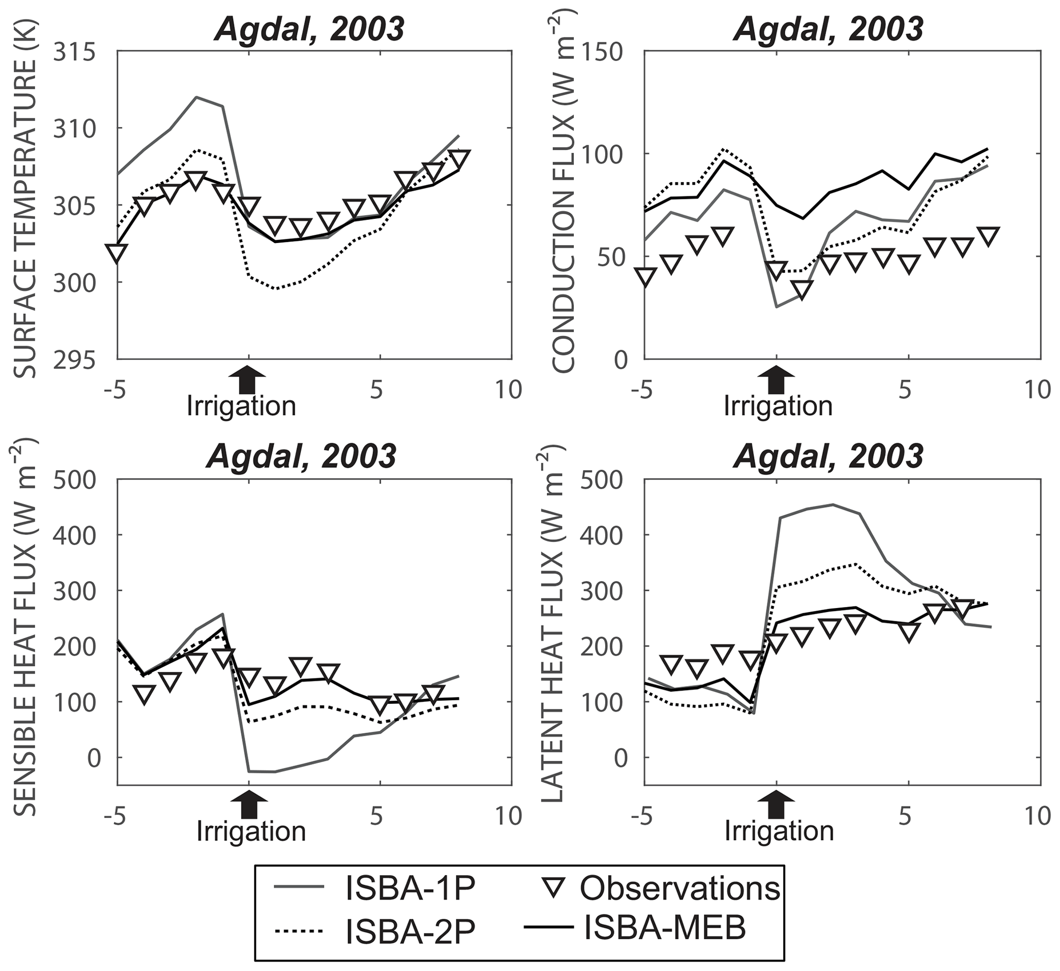
Figure 9Time series of simulated and observed surface temperature (Ts), the ground heat flux (G), and the convective heat fluxes (H and LE) during the transient regime around an irrigation event (from 5 d before irrigation and to 8 d after irrigation).
The contrast of canopy geometries between the two crops leads to significant differences of behaviour between the three configurations of the model:
-
For a homogeneous cover like wheat, the ability of all the configurations to reproduce the composite soil–vegetation heat fluxes is very close. For the latent heat flux for example, the differences between RMSEs of ISBA-1P and ISBA–MEB are about 10 W m−2 (corresponding to average error differences lower than 4 %). These results are consistent with many studies showing that the use of a composite energy balance on homogeneous cover crops is sufficient to provide a good reproduction of convective fluxes (Vogel et al., 1995; Noilhan and Mahfouf, 1996). For the olive orchard, which represents an open canopy (fraction cover of 0.55), both dual-source configurations outperformed the single-source version.
-
An analysis of the components of the uncoupled approach (ISBA-2P) shows a strong compensation between fluxes of the bare soil and the vegetation patches for the olive orchard. For instance, evapotranspiration after each irrigation event is strongly overestimated, mainly due to strong soil evaporation. This is attributed to a large available energy at the surface being directly exposed to incoming radiation coupled to an absence of root extraction for the bare soil patch. Stated differently, the aggregated flux is close to the coupled version (ISBA–MEB) and to the observations but for the wrong reasons.
In addition, another specificity of our study focused on irrigated crops in semi-arid areas as being the strong transient regime around an irrigation event, leading to a strong shift of energy between sensible and latent heat fluxes. The consequence of the differences of surface representation between the three model configurations (root distribution, available energy, heat-source coupling, etc.) leads to exacerbated consequences on the energy budget components at this time. Figure 9 summarises the behaviour of the three configurations around an irrigation event for the olive orchard. It displays the average time series of predicted and observed surface temperature (Ts), ground heat flux (G), and the convective heat fluxes (H and LE) from 5 d before to 8 d after an irrigation event. Irrigation obviously causes a drop in the composite soil/vegetation temperature (Fig. 9a). The energy is therefore mainly attributed to the latent heat flux (Fig. 9d) at the expense of the sensible heat flux (Fig. 9c). This is predicted by the three configurations of the model but with different level of accuracy. The differences in the configuration behaviours at this time explain, to a large extent, the differences in the overall performance between the simple balance configuration and the two others. ISBA-1P shows abnormally high values of LE after an irrigation event. In contrast, ISBA-2P and, above all, ISBA–MEB are able to better reproduce the observed moderate shifting.
One of the main conclusions of the study is that the new ISBA–MEB version implemented in the SURFEX platform has proved to be more suitable than single-source configuration for estimating turbulent fluxes, including evapotranspiration and its components, at least for moderately open tree canopies. This shows the need to take the interaction between vegetation and soil acting as coupled sources of heat in the parameterisation of SVATs into account when vegetation is sparse. The choice between the coupled and uncoupled model, to better represent exchanges between the biosphere and the atmosphere, is not straightforward anyway. The obtained results demonstrated that the coupled energy balance also provided the best estimates of components and composite fluxes but the patch approach followed closely. Likewise, this study also showed, as suggested by Choudhury and Monteith (1988), that the new parameters introduced in ISBA–MEB (such as the attenuation coefficient for momentum and for wind) are highly sensitive and vegetation-type dependent as evidenced by the different calibrated values between the two studied crops. This study points out the need for further local-scale evaluations on different crops of various geometries (more open rainfed sites or denser, intensive olive orchards) and for different climatic conditions in order to assess, in particular, from which degree of sparsity a dual-source approach should be preferred. This will both further our understanding of the representation of soil and vegetation heat sources in the SURFEX platform and also help to provide adequate parameterisation to global databases such as ECOCLIMAP-II, in the view of a global application of the ISBA–MEB model. Finally, considering the heavy trend towards the conversion of traditional (wheat) crops to tree crops in the southern Mediterranean region, which are more financially attractive but that consume more water (Jarlan et al., 2015), improving the representation of complex crops in the SVAT model is also of prime importance for future studies on surface–atmosphere retroaction or global change impact.
A1 Standard version
The governing equations for heat and water transfers within the soil and at the surface are given by the following formulas (more details are provided in Decharme et al., 2011):
where Tg,1 (K) is the uppermost ground temperature and Tg,i (K) is the temperature of the layer i; CT (K m−2 J−1) is the surface composite thermal inertia coefficient (Noilhan and Planton, 1989); G0 is the flux between the atmosphere and the surface; (m) and Δzi (m) are the thickness between two consecutive layer midpoints or nodes and the thickness of the layer i, respectively; Cg,i (J m−3 K−1) is the heat capacity of the soil; (W m−1 K−1) is the inverse of the weighted arithmetic mean of the soil thermal conductivity at the interface between two consecutive nodes; and vegetation is the cover fraction. Fg,i represents the vertical flow of water between layers i and i+1 and is given by Darcy's law. Eg, Dr, Pr, and R represent the amount of water evaporated from the soil (kg m−2 s−1), rainfall (kg m−2 s−1), canopy drainage (kg m−2 s−1), and surface runoff (kg m−2 s−1).
The soil heat flux, G, is defined as follows:
where is the thermal conductivity, is the thickness between the centre of the first layer and that of the second, and Ti is the temperature of the first layer and Ti+1 the temperature of the second layer.
The net radiation is calculated as follows:
where α and ε are the albedo and the emissivity, respectively, σ (W m−2 K−4) is the Stefan–Boltzmann constant, RG is the incoming solar radiation, and RA is the atmospheric radiation.
The sensible heat flux, H, is expressed as follows:
where ρa (kg m−3) is the air density, cp (J kg−1 K−1) is the specific heat of the air, Va (m s−1) is the wind speed and Ta (k−1) is air temperature, and CH is the drag coefficient.
The latent heat flux LE (W m−2), the evaporation from the soil (Eg), the direct evaporation from the foliage (Er), and the transpiration (Etr) are defined as follows:
where Lv (J kg−1) is the latent heat of vaporisation, qsat(Ts) (kg kg−1) is the saturated specific humidity at the surface temperature Ts, and qa (kg kg−1) is the atmospheric specific humidity at the lowest atmospheric level. hu is the relative humidity at the ground surface. δ is the vegetation fraction that is covered by intercepted water. Ra and Rs (s m−1) are the aerodynamic and canopy surface resistances, respectively.
Additionally, in this study, ISBA uses the A−gs parameterisation to estimate the stomatal conductance gs by considering the impact of the atmospheric carbon dioxide concentration and the interactions between all environmental factors on the stomatal aperture. Therefore, the leaf stomatal conductance is expressed as follows (Calvet et al., 1998):
where gc (mm s−1) is the cuticular conductance, An (mg m−2 s−1) is the net assimilation, and Amin is the rate of the residual photosynthesis rate (at full light intensity). Cs and Ci are the internal and air CO2 concentrations, respectively. Ds and are the leaf-to-air saturation deficits, and is the maximum leaf-to-air saturation deficit, respectively. Am is the photosynthesis rate in light-saturating conditions.
The gs is multiplied by the leaf area index (LAI) value in order to scale up gs from the leaf to the canopy. Finally, the integrated canopy net assimilation AnI and conductance gsI, which were used to compute the heat and water vapour surface fluxes and the canopy resistance, respectively, are then written by assuming a homogeneous leaf vertical distribution as follows:
where h is the height of the canopy and z is the distance to the soil.
A2 ISBA Multiple energy balance (MEB)
Compared to ISBA standard, MEB distinguishes the soil and the vegetation surface temperatures. Fluxes from the ground or vegetation first transit to the so-called canopy air space or canopy before being in contact with the atmosphere. For extended details about the prognostic equations and its numerical resolution aspects and the various assumptions of the MEB version, one can refer to Boone et al. (2017). We develop in the following paragraphs, the main equations and parameterisations that will be used for this study. As soil freeze thaw is negligible for this study (no snow process is involved), the related terms will be not presented.
The prognostic equations for the energy budget are as follows:
where Tg,1 is the uppermost ground temperature, and Tv is the bulk canopy temperature (K). The subscripts 1, v, and g indicate the uppermost layer, vegetation canopy, and ground, respectively. The ISBA–MEB sensible heat fluxes, Hv (between the vegetation and canopy air space), Hg (between the ground and canopy) and Hc (between the canopy and the overlaying atmosphere) are defined as follows:
Rag-c, Rav-c, and Rac-c are the aerodynamic resistances to heat transfer between the canopy and the ground (Choudhury and Monteith, 1988), the canopy and the vegetation, and the atmosphere and the canopy, respectively. Γ (J kg−1) is a thermodynamic variable which is expressed as a linear relationship with the temperature (Boone et al., 2017). Note that in the model code, potential temperature or dry static energy are used as thermodynamic variables but, for simplicity, these quantities have been approximated using temperature (since the impact of this approximation is quite small in the current study).
The ISBA–MEB latent heat fluxes, Ev (between the vegetation and canopy), Eg (between the ground and canopy), and Ec (between the canopy and the overlaying atmosphere) are defined as follows:
where hsv is the Halstead coefficient.
In what follows, we present the main parameterisations introduced to calculate the new parameters needed by the model as the fraction of the vegetation covered with intercepted water:
The maximum water interception storage in the capacity of the vegetation is simply defined as follows:
with cwrv=0.2.
The canopy absorption is defined as follows:
where τLW represents a long-wave radiation transmission factor that can be species (or land classification) dependent.
The aerodynamic resistance between the vegetation canopy and the surrounding air space is defined as follows:
The bulk canopy aerodynamic conductance gav between the canopy and the canopy air is parameterised as follows (Choudhury and Monteith, 1988):
where uhv is the wind speed at the top of the canopy (m s−1), lw is the leaf width, αav is the canopy conductance scale factor, and is the attenuation coefficient for wind.
The MEB code is part of the ISBA LSM and is available as open-source code via the surface modelling platform called SURFEX, which can be downloaded at http://www.cnrm-game-meteo.fr/surfex/ (SURFEX, 2020). SURFEX is updated at a relatively low frequency (every 3–6 months), and the developments presented in this paper are available starting with SURFEX version 8.0. If more frequent updates are needed, or if what is required is not in Open-SURFEX (DrHOOK, FA/LFI formats, and GAUSSIAN grid), you are invited to follow the procedure (see the instructions at the previous link) to obtain an SVN account to access the real-time modifications of the code. The validation data for both sites are available on request from the coleads of the Tensift observatory, namely Jamal Ezzahar (j.ezzahar@uca.ma) and Vincent Simonneaux (vincent.simonneaux@ird.fr).
The supplement related to this article is available online at: https://doi.org/10.5194/hess-24-3789-2020-supplement.
GA and LJ worked out almost all of the technical details, performed the numerical calculations for the suggested experiment, and took the lead in writing the paper. LJ, JE, and ABo conceived the original idea and supervised the findings of this work. SE, ABe, SK, GB, SG, AC, ABo, and AN contributed to the interpretation of the results and to the final version of the paper. ABo and AN designed the model and the computational framework. All authors provided critical feedback and helped shape the research, analysis, and paper.
The authors declare that they have no conflict of interest.
This article is part of the special issue “Changes in the Mediterranean hydrology: observation and modeling”. It is not associated with a conference.
This research has been carried out within the framework of the joint international TREMA (a collaboration between IRD, UCAM, DMN, CNESTEN, ABHT, and ORMVAH) and the ERANET-MED 03-62 CHAAMS project. Ghizlane Aouade was awarded a scholarship by the MISTRAL/SICMED2 programme. She also received travel grants from the MISTRALS/ENVI-MED programme through the CHAMO project, from the PHC Toubkal (grant no. TBK/18/61) and from the Research and Innovation Staff Exchange (RISE) REC project (grant no. H2020/645642) financed by Maria Skłodowska-Curie research.
Financial support for the experiment was provided by IRD, the MISTRALS/SICMED programme through the MetaSim project, the ANR AMETHYST project (grant no. ANR-12-TMED-0006-01), and the Sagesse project (Projet Prioritaire de Recherche (PPR) Type B) funded by the Minister for Higher Education, Scientific Research and Executive Training (Morocco). This work was also supported by the Horizon 2020 Partnership for Research and Innovation in the Mediterranean Area (PRIMA) ALTOS project.
This paper was edited by María José Polo and reviewed by Pierre Gentine and one anonymous referee.
Aouade, G., Ezzahar, J., Amenzou, N., Er-Raki, S., Benkaddour, A., Khabba, S., and Jarlan, L.: Combining stable isotopes and micrometeorological measurements for partitioning evapotranspiration of winter wheat into soil evaporation and plant transpiration in a semi-arid region, Agr. Water Manage., 177, 181–192, 2016.
Bastidas, L. A., Gupta, H. V., Sorooshian, S, Shuttleworth, W. J., and Yang, Z. L.: Sensitivity analysis of a land surface scheme using multicriteria methods, J. Geophys. Res., 104, 19481–19490, 1999.
Béziat, P., Rivalland, V., Tallec, T., Jarosz, N., Boulet, G., Gentine, P., and Ceschia, E.: Evaluation of a simple approach for crop evapotranspiration partitioning and analysis of the water budget distribution for several crop species, Agr. Forest Meteorol., 177, 46–56, 2013.
Blyth, E. M. and Harding, R. J.: Application of aggregation models to surface heat flux from the Sahelian tiger bush, Agr. Forest Meteorol., 72, 213–235, 1995.
Blyth, E. M., Harding, R. J., and Essery, R.: A coupled dual source GCM SVAT, Hydrol. Earth Syst. Sci., 3, 71–84, https://doi.org/10.5194/hess-3-71-1999, 1999.
Boone, A., Calvet, J., and Noilhan, J.: Inclusion of a third soil layer in a land surface scheme using the force-restore method, J. Appl. Meteorol., 38, 1611–1630, 1999.
Boone, A., De Rosnay, P., Balsamo, G., Beljaars, A., Chopin, F., Decharme, B., Delire, C., Ducharne, A., Gascoin, S., and Grippa, M.: The amma land surface model intercomparison project (almip), B. Am. Meteorol. Soc., 90, 1865–1880, 2009.
Boone, A., Samuelsson, P., Gollvik, S., Napoly, A., Jarlan, L., Brun, E., and Decharme, B.: The interactions between soil–biosphere–atmosphere land surface model with a multi-energy balance (ISBA-MEB) option in SURFEXv8 – Part 1: Model description, Geosci. Model Dev., 10, 843–872, https://doi.org/10.5194/gmd-10-843-2017, 2017.
Boulet, G., Chehbouni, A., Braud, I., and Vauclin, M.: Mosaic versus dual source approaches for modelling the surface energy balance of a semi-arid land, Hydrol. Earth Syst. Sci., 3, 247–258, https://doi.org/10.5194/hess-3-247-1999, 1999.
Boulet, G., Chehbouni, A., Gentine, P., Duchemin, B., Ezzahar, J., and Hadria, R.: Monitoring water stress using time series of observed to unstressed surface temperature difference, Agr. Forest Meteorol., 146, 159–172, 2007.
Boulet, G., Mougenot, B., Lhomme, J.-P., Fanise, P., Lili-Chabaane, Z., Olioso, A., Bahir, M., Rivalland, V., Jarlan, L., Merlin, O., Coudert, B., Er-Raki, S., and Lagouarde, J.-P.: The SPARSE model for the prediction of water stress and evapotranspiration components from thermal infra-red data and its evaluation over irrigated and rainfed wheat, Hydrol. Earth Syst. Sci., 19, 4653–4672, https://doi.org/10.5194/hess-19-4653-2015, 2015.
Braud, I., Dantas-Antonino, A. C., Vauclin, M., Thony, J. L., and Ruelle, P.: A simple soil-plant-atmosphere transfer model (SiSPAT) development and field verification, J. Hydrol., 166, 213–250, 1995.
Brooks, R. H. and Corey, A. T.: Properties of porous media affecting fluid flow, J. Irrig. Drain. Am. Soc. Civ. Eng.. 17, 187–208, 1966.
Calvet, J. C.: Investigating soil and atmospheric plant water stress using physiological and micrometeorological data, Agr. Forest Meteorol., 103, 229–247, 2000.
Calvet, J. C. and Soussana, J.-F.: Modelling CO2-enrichment effects using an interactive vegetation SVAT scheme, Agr. Forest Meteorol., 108, 129–152, 2001.
Calvet, J.-C., Noilhan, J., Roujean, J.-L., Bessemoulin, P., Cabelguenne, M., Olioso, A., and Wigneron, J.-P.: An interactive vegetation svat model tested against data from six contrasting sites, Agr. Forest Meteorol., 92, 73–95, 1998.
Calvet, J.-C., Rivalland, V., Picon-Cochard, C., and Guehl, J.-M.: Modelling forest transpiration and CO2 fluxes – response to soil moisture stress, Agr. Forest Meteorol., 124, 143–156, https://doi.org/10.1016/j.agrformet.2004.01.007, 2004.
Calvet, J.-C., Gibelin, A.-L., Roujean, J.-L., Martin, E., Le Moigne, P., Douville, H., and Noilhan, J.: Past and future scenarios of the effect of carbon dioxide on plant growth and transpiration for three vegetation types of southwestern France, Atmos. Chem. Phys., 8, 397–406, https://doi.org/10.5194/acp-8-397-2008, 2008.
Carrer, D., Roujean, J.-L., Lafont, S., Calvet, J.-C., Boone, A., Decharme, B., Delire, C., and Gastellu-Etchegorry, J.-P.: A canopy radiative transfer scheme with explicit fapar for the interactive vegetation model isba-a-gs: Impact on carbon fluxes, J. Geophys. Res., 118, 888–903, 2013.
Chehbouni, A., Escadafal, R., Duchemin, B., Boulet, G., Simonneaux, V., Dedieu, G., Mougenot, B., Khabba, S., Kharrou, H., Maisongrande, P., Merlin, O., Chaponnière, A., Ezzahar, J., Er-Raki, S., Hoedjes, J., Hadria, R., Abourida, A., Cheggour, A., Raibi F., Boudhar, A., Benhadj, I, Hanich, L., Benkaddour, A., Guemouria, N., Chehbouni, A., Lahrouni, A., Olioso, A., Jacob, F., Williams, D. G., and Sobrino, J.: An integrated modelling and remote sensing approach for hydrological study in arid and semi-arid regions: the SUDMED Programme, Int. J. Remote Sens., 29, 5161–5181, 2008.
Choudhury, B. J. and Idso, S. B.: An empirical model for stomatal resistance of field-grown wheat, Agr. Forest Meteorol., 36, 65–82, 1985.
Choudhury, B. J. and Monteith, J. L.: A four-layer model for the heat budget of homogeneous land surfaces, Q. J. Roy. Meteorol. Soc., 114, 373–398, 1988.
Clapp, R. B. and Hornberger, G. M.: Empirical equations for some soil hydraulic properties, Water Resour. Res., 14, 601–604, 1978.
Cosby, B. J., Hornberger, G. M., Clapp, R. B., and Ginn, T. R.: A statistical exploration of soil moisture characteristics to the physical properties of soils, Water Resour. Res., 20, 682–690, 1984.
Coudert, B., Ottlé, C., Boudevillain, B., Demarty, J., and Guillevic, P.: Contribution of Thermal Infrared Remote Sensing Data in Multiobjective Calibration of a Dual-Source SVAT Model, J. Hydrometeorol., 7, 404–420, 2006.
Deardorff, J. W.: A parameterization of ground-surface moisture content for use in atmosphere prediction models, J. Appl. Meteorol., 16, 1182–1185, 1977.
Decharme, B., Boone, A., Delire, C., and Noilhan, J.: Local evaluation of the interaction between soil biosphere atmosphere soil multilayer diffusion scheme using four pedotransfer functions, J. Geophys. Res., 116, 1–29, https://doi.org/10.1029/2011JD016002, 2011.
Decharme, B., Martin, E., and Faroux, S.: Reconciling soil thermal and hydrological lower boundary conditions in land surface models, J. Geophys. Res.-Atmos., 118, 7819–7834, https://doi.org/10.1002/jgrd.50631, 2013.
Demarty, J.: Développement et application du modèle SiSPAT-RS à l'échelle de la parcelle et dans le cadre de l'expérience alpilles ReSeDA. Thèse de doctorat de l'université Denis Diderot de Paris 7, Paris, France, p. 221, 2001.
Demarty, J., Ottlé, C., Braud, I., Olioso, A., Frangi, J. P., Gupta, H. V., and Bastidas, L. A.: Constraining a physically based Soil-Vegetation-Atmosphere Transfer model with surface water content and thermal infrared brightness temperature measurements using a multiobjective approach, Water Resour. Res., 41, W01011, https://doi.org/10.1029/2004WR003695, 2005.
Duchemin, B., Hadria, R., Er-Raki, S., Boulet, G., Maisongrande, P., Chehbouni, A., Escadafal, R., Ezzahar, J., Hoedjes, J. C. B., Karrou, H., Khabba, S., Mougenot, B., Olioso, A., Rodriguez, J.-C., and Simonneaux, V.: Monitoring wheat phenology and irrigation in Central Morocco: on the use of relationship between evapotranspiration, crops coefficients, leaf area index and remotely-sensed vegetation indices, Agr. Water Manage., 79, 1–27, 2006.
Duchemin, B., Hagolle, O., Mougenot, B., Simonneaux, V., Benhadj, I., Hadria, R., Ezzahar, J., Hoedjes, J., Khabba, S., Kharrou, M. H., Boulet, G., Dedieu, G., Er-Raki S., Escadafal, R., Olioso, A., and Chehbouni, A. G.: Agrometerological study of semi-arid areas: an experiment for analysing the potential of FORMOSAT-2 time series of images in the Tensift-Marrakech plain, Int. J. Remote Sens., 29, 5291–5299, 2008.
Eltahir, E. A. B. and Bras, R. L.: Precipitation Recycling, Rev. Geophys., 34, 367–378, https://doi.org/10.1029/96rg01927, 1996.
Er-Raki, S., Chehbouni, A., Guemouria, N., Duchemin, B., Ezzahar, J., and Hadria, R.: Combining FAO-56 model and ground-based remote sensing to estimate water consumptions of wheat crops in a semi-arid region, Agr. Water Manage., 87, 41–54, 2007.
Er-Raki, S., Chehbouni, A., Boulet, G., and Williams, D. G.: Using the dual approach of FAO-56 for partitioning ET into soil and plant components for olive orchards in a semi-arid region, Agr. Water Manage., 97, 1769–1778, 2010.
Ezzahar, J., Chehbouni, A., Hoedjes, J. C. B., Er-Raki, S., Chehbouni, A., Bonnefond, J.-M., and De Bruin, H. A. R.: The use of the Scintillation Technique for estimating and monitoring water consumption of olive orchards in a semi-arid region, Agr. Water Manage., 89, 173–184, 2007a.
Ezzahar, J., Chehbouni, A., Hoedjes, J. C. B., and Chehbouni, A.: On the application of scintillometry over heterogeneous surfaces, J. Hydrol., 334, 493–501, 2007b.
Ezzahar, J. and Chehbouni A: The use of the scintillometry for validating the spatial and temporal aggregation schema over heterogeneous grid. Agricultural and Forest Meteorology, vol. 149, pp. 2098-2109, 2009.
Ezzahar, J., Chehbouni, A., Er-Raki, S., and Hanich, L.: Combining a Large Aperture Scintillometer and estimates of available energy to derive evapotranspiration over several agricultural fields in semi-arid regions, Plant Biosyst., 143, 209–221, 2009.
Faroux, S., Kaptué Tchuenté, A. T., Roujean, J.-L., Masson, V., Martin, E., and Le Moigne, P.: ECOCLIMAP-II/Europe: a twofold database of ecosystems and surface parameters at 1 km resolution based on satellite information for use in land surface, meteorological and climate models, Geosci. Model Dev., 6, 563–582, https://doi.org/10.5194/gmd-6-563-2013, 2013.
Fernández, J. E., Palomo, M. J., Díaz-Espejo, A., Clothier, B. E., Green, S. R., Girón, I. F., and Moreno, F.: Heat-pulse measurements of sap flow in olives for automating irrigation: tests, root flow and diagnostics of water stress, Agr. Water Manage., 51, 99–123, 2001.
Fernández, J. E., Moreno, F., and Martin-Aranda, J.: Study of root dynamics of olive trees under drip irrigation and dry farming, Acta Hortic., 286, 263–266, 1990.
Garratt, J. R.: The Atmospheric Boundary Layer, Cambridge University Press, Cambridge, UK, 316 pp., 1992.
Garrigues, S., Olioso, A., Carrer, D., Decharme, B., Calvet, J.-C., Martin, E., Moulin, S., and Marloie, O.: Impact of climate, vegetation, soil and crop management variables on multi-year ISBA-A-gs simulations of evapotranspiration over a Mediterranean crop site, Geosci. Model Dev., 8, 3033–3053, https://doi.org/10.5194/gmd-8-3033-2015, 2015.
Garrigues S., Boone, A., Decharme, B., Olioso, A., Albergel, C., Calvet, J.-C., Moulin, S., Buis, S., and Martin, E.: Impacts of the Soil Water Transfer Parameterization on the Simulation of Evapotranspiration over a 14-Year Mediterranean Crop Succession, J. Hydro-Meteorol., 19, 3–25, 2018.
Gentine, P., Entekhabi, D. Chehbouni, A., Boulet, G., and Duchemin, B.: Analysis of evaporative fraction diurnal behaviour, Agr. Forest Meteorol., 143, 13–29, 2007.
Gibelin, A. L., Calvet, J. C., Roujean, J. L., Jarlan, L., and Los, S. O.: Ability of the land surface model ISBA-A-gs to simulate leaf area index at the global scale: Comparison with satellites products, J. Geophys. Res., 111, D18102, https://doi.org/10.1029/2005JD006691, 2006.
Giordani, H., Noilhan, J., Lacarrere, P., and Bessemoulin, P.: Modeling the surface processes and the atmospheric boundary layer for semi-arid conditions, Agr. Forest Meteorol., 80, 263–287, 1996.
Goldberg, D. E.: Genetic algorithms in Search, Optimization and Machine learning, Addison-Wesley Publishing Co, Reading, MA, 412 pp., 1989.
Habets, F., Boone, A., Champeaux, J.-L., Etchevers, P., Franchisteguy, L., Leblois, E., Ledoux, E., Le Moigne, P., Martin, E., Morel, S., Noilhan, J., Quintana Seguí, P., Rousset-Regimbeau, F., and Viennot, P.: The SAFRAN-ISBA-MODCOU hydrometeorological model applied over France, J. Geophys. Res., 113, D06113, https://doi.org/10.1029/2007JD008548, 2008.
Hartmann, D. L.: Global Physical Climatology, Elsevier, Amsterdam, the Netherlands, 498 pp., https://doi.org/10.1016/B978-0-12-328531-7.00011-6, 2016.
Hoedjes, J. C. B., Chehbouni, A., Ezzahar, J., Escadafal, R., and De Bruin, H. A. R.: Comparison of Large Aperture Scintillometer and Eddy Covariance Measurements: Can Thermal Infrared Data be Used to Capture Footprint Induced Differences, J. Hydrometeorol., 8, 144–159, 2007.
Hoedjes, J. C. B., Chehbouni, A., Jacob, F., Ezzahar, J., and Boulet, G.: Deriving daily evapotranspiration from remotely sensed instantaneous evaporative fraction over olive orchard in semi-arid Morocco, J. Hydrol., 354, 53–64, 2008.
Jackson, R. B., Canadell, J., Ehleringer, J. R., Mooney, H. A., Sala, O. E., and Schulze, E. D.: A global analysis of root distributions for terrestrial biomes, Oecologia, 108, 389–411, https://doi.org/10.1007/BF00333714, 1996.
Jarlan, L., Khabba, S., Er-Raki, S., and Le Page, M.: Remote Sensing of Water Resources in Semi-Arid Mediterranean Areas: the joint international laboratory TREMA, Int. J. Remote Sens., 36, 4879–4917, https://doi.org/10.1080/01431161.2015.1093198, 2015.
Jasechko, S., Sharp, Z. D., Gibson, J. J., Birks, S. J., Yi, Y., and Fawcett, P. J.: Terrestrial water fluxes dominated by transpiration, Nature, 496, 347–350, https://doi.org/10.1038/nature11983, 2013.
Jiménez, C., Prigent, C., Mueller, B., Seneviratne, S. I., McCabe, M. F., Wood, E. F., Rossow, W. B., Balsamo, G., Betts, A. K., Dirmeyer, P. A., Fisher, J. B., Jung, M., Kanamitsu, M., Reichle, R. H., Reichstein, M., Rodell, M., Sheffield, J., Tu, K., and Wang, K.: Global intercomparison of 12 land surface heat flux estimates, J. Geophys. Res., 116, D02102, https://doi.org/10.1029/2010JD014545, 2011.
Kalma, J. D. and Jupp, D. L. B.: Estimating evaporation from pasture using infrared thermometry: evaluation of a one-layer resistance model, Agr. Forest Meteorol., 51, 223–246, https://doi.org/10.1016/0168-1923(90)90110-R, 1990.
Kool, D., Agam, N., Lazarovitch, N., Heitman, J. L., Sauer, T. J., and Ben-Gal, A.: A review of approaches for evapotranspiration partitioning, Agr. Forest Meteorol., 184, 56–70, https://doi.org/10.1016/j.agrformet.2013.09.003, 2014.
Lawston, P. M., Santanello, J. A., Zaitchik, B., and Rodell, M.: Impact of irrigation methods on land surface model spinup and initialization of WRF forecasts, J. Hydrometeorol., 16, 1135–1154, https://doi.org/10.1175/JHM-D-14-0203.1, 2015.
Lei, H. and Yang, D.: Interannual and seasonal variability in evapotranspiration and energy partitioning over an irrigated cropland in the North China Plain, Agr. Forest Meteorol., 150, 581–589, 2010.
Le Page, M., Toumi, J., Khabba, S., Hagolle, O., Tavernier, A., Kharrou, M. H., Er-Raki, S., Huc, M., Kasbani, M., Moutamanni, A. E., Yousfi, M., and Jarlan, L.: A Life-Size and Near Real-Time Test of Irrigation Scheduling with a Sentinel-2 Like Time Series (SPOT4-Take5) in Morocco, Remote Sens., 6, 11182–11203, 2014.
Lhomme, J.-P. and Chehbouni A.: Comments on dual-source vegetation-atmosphere transfer models, Agr. Forest Meteorol., 94, 269–273, 1999.
Lhomme, J.-P., Monteny, B., and Amadou, M.: Estimating sensible heat flux from radiometric temperature over sparse millet, Agr. Forest Meteorol., 68, 77–91, 1994.
Lhomme, J. P., Troufleau, D., Monteny, B., Chehbouni, A., and Bauduin, S.: Sensible heat flux–radiometric surfacetemperature over sparse Sahelian vegetation. II. A model for the kB−1 parameter, J. Hydrol., 188–189, 839–854, 1997.
Lhomme, J. P., Montes, C., Jacob, F., and Prévot, L.: Evaporation from heterogeneous and sparse canopies: on the formulations related to multi-source representations, Bound.-Lay. Meteorol., 144, 243–262, 2012.
Maillard, P.: L'olivier, Comité technique de l'olivier section spécialise de l'INVFLEC, Institut National de Vulgarisation pour les Fruits, Légumes et Champignions, Paris, p. 137, 1975.
Masson, V., Le Moigne, P., Martin, E., Faroux, S., Alias, A., Alkama, R., Belamari, S., Barbu, A., Boone, A., Bouyssel, F., Brousseau, P., Brun, E., Calvet, J.-C., Carrer, D., Decharme, B., Delire, C., Donier, S., Essaouini, K., Gibelin, A.-L., Giordani, H., Habets, F., Jidane, M., Kerdraon, G., Kourzeneva, E., Lafaysse, M., Lafont, S., Lebeaupin Brossier, C., Lemonsu, A., Mahfouf, J.-F., Marguinaud, P., Mokhtari, M., Morin, S., Pigeon, G., Salgado, R., Seity, Y., Taillefer, F., Tanguy, G., Tulet, P., Vincendon, B., Vionnet, V., and Voldoire, A.: The SURFEXv7.2 land and ocean surface platform for coupled or offline simulation of earth surface variables and fluxes, Geosci. Model Dev., 6, 929–960, https://doi.org/10.5194/gmd-6-929-2013, 2013.
Napoly, A., Boone, A., Samuelsson, P., Gollvik, S., Martin, E., Seferian, R., Carrer, D., Decharme, B., and Jarlan, L.: The interactions between soil–biosphere–atmosphere (ISBA) land surface model multi-energy balance (MEB) option in SURFEXv8 – Part 2: Introduction of a litter formulation and model evaluation for local-scale forest sites, Geosci. Model Dev., 10, 1621–1644, https://doi.org/10.5194/gmd-10-1621-2017, 2017.
Noilhan, J. and Mahfouf, J.-F.: The ISBA land surface parameterisation scheme, Global Planet. Change, 13, 145–159, 1996.
Noilhan, J. and Planton, S.: A simple parameterization of land surface processes for meteorological models, Mon. Weather Rev., 117, 536–549, 1989.
Norman, J. M., Kustas, W. P., and Humes, K. S.: Two source approach for estimating soil and vegetation energy fluxes in observations of directional radiometric surface temperature, Agr. Forest Meteorol., 77, 263–293, 1995.
Oishi, A. C., Oren, R., and Stoy, P. C.: Estimating components of forest evapotranspiration: a footprint approach for scaling sapflux measurements, Agr. Forest Meteorol., 148, 1719–1732, 2008.
Ozdogan, M., Rodell, M., Beaudoing, H. K., and Toll, D. L.: Simulating the effects of irrigation over the United States in a land surface model based on satellite-derived agricultural data, J. Hydrometeorol., 11, 171–184, https://doi.org/10.1175/2009JHM1116.1, 2010.
Pianosi, F., Wagener, T., Rougier, J., Freer, J., and Hall, J.: Sensitivity analysis of environmental models: a systematic review with practical workflow, in: Vulnerability, Uncertainty, and Risk, American Society of Civil Engineers, Reston, USA, 290–299, 2014.
Raupach, M. R. and Finnigan, J. J.: Single-layer models of evaporation from plant canopies are incorrect but useful, whereas multilayer models are correct but useless: discuss, Aust. J. Plant Physiol., 15, 705–716, 1988.
Rivalland, V., Calvet, J.-Ch., Berbigier, P., Brunet, Y., and Granier, A.: Transpiration and CO2 fluxes of a pine forest: modelling the undergrowth effect, Ann. Geophys., 23, 291–304, https://doi.org/10.5194/angeo-23-291-2005, 2005.
Rowntree, P. R.: Atmospheric parametrization schemes for evaporation over land: basic concepts and climate modeling aspects, in: land surface evaporation: measurements and parametrization, edited by: Schmugge, T. J. and Andre, J. C., Springer-Verlag, New York, 5–29, 1991.
Sellers, P. J., Los, S. O., and Tucker, C. J.: A revised land-surface parameterization (SiB2) for atmospheric GCMs. Part 2: The generation of global fields of terrestrial biophysical parameters from satellite data, J. Climate, 9, 706–737, 1996.
Shuttleworth, W. J. and Gurney, R. J.: The theoretical relationship between foliage temperature and canopy resistance in sparse crops, Q. J. Roy. Meteorol. Soc., 116, 497–519, 1990.
Shuttleworth, W. J. and Wallace, J. S.: Evaporation from sparse crops-an energy combination theory, Q. J. Roy. Meteorol. Soc., 111, 839–855, 1985.
SURFEX: available at: http://www.cnrm-game-meteo.fr/surfex/, last access: 22 July 2020.
Taylor, K. E.: Summarizing multiple aspects of model performance in a single diagram, J. Geophys. Res., 106, 7183–7192, 2001.
Twine, T. E., Kustas, W. P., Norman, J. M., Cook, D. R., Houser, P. R., Meyers, T. P., Prueger, J. H., Starks, P. J., and Wesly, M. L.: Correcting Eddy-Covariance Flux Underestimates over a Grassland, Agric. Forest Meteorol., 103, 279–300, 2000.
Van den Hurk, B. J. J. M. and McNaughton, K. G.: Implementation of near-field dispersion in a simple two-layer surface resistance model, J. Hydrol., 166, 293–311, 1995.
Vogel, C. A., Baldocchi, D. D., Luhar, A. K., and Rao, K. S.: A Comparison of a Hierarchy of Models for Determining Energy Balance Components over Vegetation Canopies, J. Appl. Meteorol., 34, 2182–2196, 1995.
Voltz, M., Ludwig, W., Leduc, C., and Bouarfa, S.: Mediterranean land systems under global change: current state and future challenges, Reg. Environ. Change, 18, 619–622, 2018.
Wang, W. G., Xing, W. Q., Shao, Q. X., Yu, Z. B., Peng, S. Z., Yang, T., Yong, B., Taylor, J., and Singh, V. P.: Changes in reference evapotranspiration across the Tibetan Plateau: Observations and future projections based on statistical downscaling, J. Geophys. Res.-Atmos., 118, 4049–4068, https://doi.org/10.1002/jgrd.50393, 2013.
Williams, D. G., Cable, W., Hultine, K., Hoedjes, J. C. B., Yepez, E. A., Simonneaux, V., Er-Raki, S., Boulet, G., de Bruin, H. A. R., Chehbouni, A., Hartogensis, O. K., and Timouk, F.: Components of evapotranspiration in an olive orchard determined by eddy covariance, sap flow and stable isotope techniques, Agr. Forest Meteorol., 125, 241–258, 2004.
Xu, C. Y. and Singh, V. P.: Evaluation of three complementary relationship evapotranspiration models by water balance approach to estimate actual regional evapotranspiration in different climatic regions, J. Hydrol., 308, 105–121, https://doi.org/10.1016/j.jhydrol.2004.10.024, 2005.
Xu, C. Y., Widén, E., and Halldin, S.: Modelling hydrological consequences of climate change-progress and challenges, Adv. Atmos. Sci., 22, 789–797, https://doi.org/10.1007/BF02918679, 2005.
- Abstract
- Introduction
- Data and land surface model ISBA-A-gs
- Results
- Discussion and conclusion
- Appendix A: Prognostic equations of ISBA-A-gs
- Code and data availability
- Author contributions
- Competing interests
- Special issue statement
- Acknowledgements
- Financial support
- Review statement
- References
- Supplement