Multi-constellation GNSS interferometric reflectometry with mass-market sensors as a solution for soil moisture monitoring

Per capita arable land is decreasing due to the rapidly increasing population, and fresh water is becoming scarce and more expensive. Therefore, farmers should continue to use technology and innovative solutions to improve efficiency, save input costs, and optimise environmental resources (such as water). In the case study presented in this paper, the Global Navigation Satellite System interferometric reflectometry (GNSS-IR) technique was used to monitor soil moisture during 66 d, from 3 December 2018 to 6 February 2019, in the installations of the Cajamar Centre of Experiences, Paiporta, Valencia, Spain. Two main objectives were pursued. The first was the extension of the technique to a multi-constellation solution using GPS, GLONASS, and GALILEO satellites, and the second was to test whether mass-market sensors could be used for this technique. Both objectives were achieved. At the same time that the GNSS observations were made, soil samples taken at 5 cm depth were used for soil moisture determination to establish a reference data set. Based on a comparison with that reference data set, all GNSS solutions, including the three constellations and the two sensors (geodetic and mass market), were highly correlated, with a correlation coefficient between 0.7 and 0.85.

1 Introduction

Soil moisture is a fundamental component of the hydrological cycle and a key observable variable for optimising agricultural irrigation management. Additionally, soil moisture monitoring has been one of the main goals of the remote sensing satellite missions of Soil Moisture and Ocean Salinity (SMOS; Kerr et al., 2001), Soil Moisture Active Passive (SMAP; Chan et al., 2016), and Sentinel-1 (Mattia et al., 2018). These missions are used to used to derive global maps of soil moisture. SMOS does so every 3 d at a spatial resolution of about 50 km, SMAP every 2–3 d, with a spatial resolution of about 40 km (gridded to 36 km since the radiometer is the only instrument onboard that works), and one Sentinel-1 satellite every 12 d (two Sentinel-1 satellites are in orbit, which decreases the revisit time), with a spatial resolution of about 1 km.

To obtain information about soil moisture at a very local scale and continuously, the Global Navigation Satellite System (GNSS) reflectometry began to be tested as a possible solution (Masters et al., 2002; Zavorotny et al., 2003; Katzberg et al., 2005). This was possible because GNSS satellites transmit in the L band (microwave frequency), so the GNSS signal reflected by nearby surfaces and recorded by the antenna contains information about the environment surrounding the antenna (scale of about 1000 m²). In particular, the ground-reflected global positioning system signal measured by a geodetic-quality GNSS system can be used to infer temporal changes in near-surface soil moisture. This technique, known as GNSS interferometric reflectometry (GNSS-IR), analyses changes in the interference pattern of the direct and reflected signals (Fig. 1), which are recorded in signal-to-noise ratio (SNR) data, as being interferograms. Thus, GNSS-IR can be considered as another remote sensing technique for monitoring soil moisture in a local scale and continuously, independent of climatological conditions (the technique is valid in rainy and foggy conditions) and illumination (day or night). Temporal fluctuations in the phase of the interferogram are indicative of changes in near-surface (depth of about 5–7 cm) volumetric soil moisture content (Larson et al., 2008a, b).

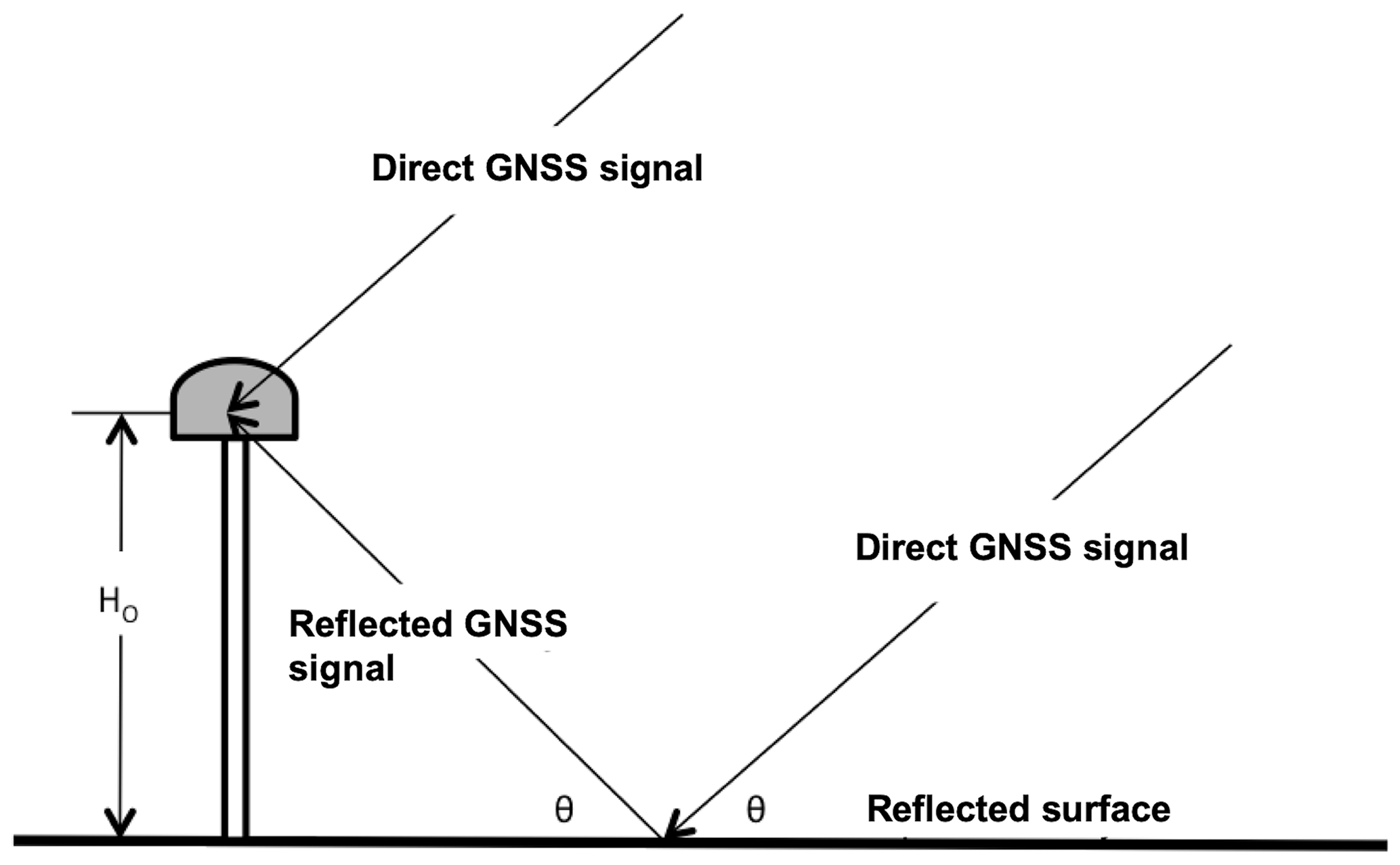
Figure 1 Principle of the Global Navigation Satellite System interferometric reflectometry (GNSS-IR). H_O is the antenna height and θ it the satellite elevation angle.

Commercially available geodetic-quality GNSS receivers and antennas can be used for GNSS-IR. The method has been tested with the Global Positioning System (GPS) satellite constellation, and it has been shown to provide consistent measurements of the upper surface soil moisture content (Larson et al., 2008a, b, 2010; Larson and Nievinski, 2013; Chew et al., 2014, 2015, 2016; Small et al., 2016; Vey et al., 2016; Wan et al., 2015; Chen et al., 2016; Zhang et al., 2017).

With the use of the GPS constellation, the GPS-IR reflection footprint is far from homogeneous, Fig. 2, and some tracks cannot be included in the process and analysis (Vey et al., 2016; Chew et al., 2016). Therefore, GPS-IR needs to evolve to Global Navigation Satellite System reflectometry (GNSS-IR), where multi-constellation observation provides the solution. The integration of new navigation satellite constellations will produce a more homogeneous footprint around the antenna (Fig. 2). Roussel et al. (2016) introduced the GLONASS Russian constellation to retrieve soil moisture over bare soil, but there are no references in the literature to the European GALILEO or Chinese BEIDU constellations. Roesler and Larson (2018) provided a software tool for generating map GNSS-IR reflection zones that support GPS, GLONASS, GALILEO, and BEIDU constellations.

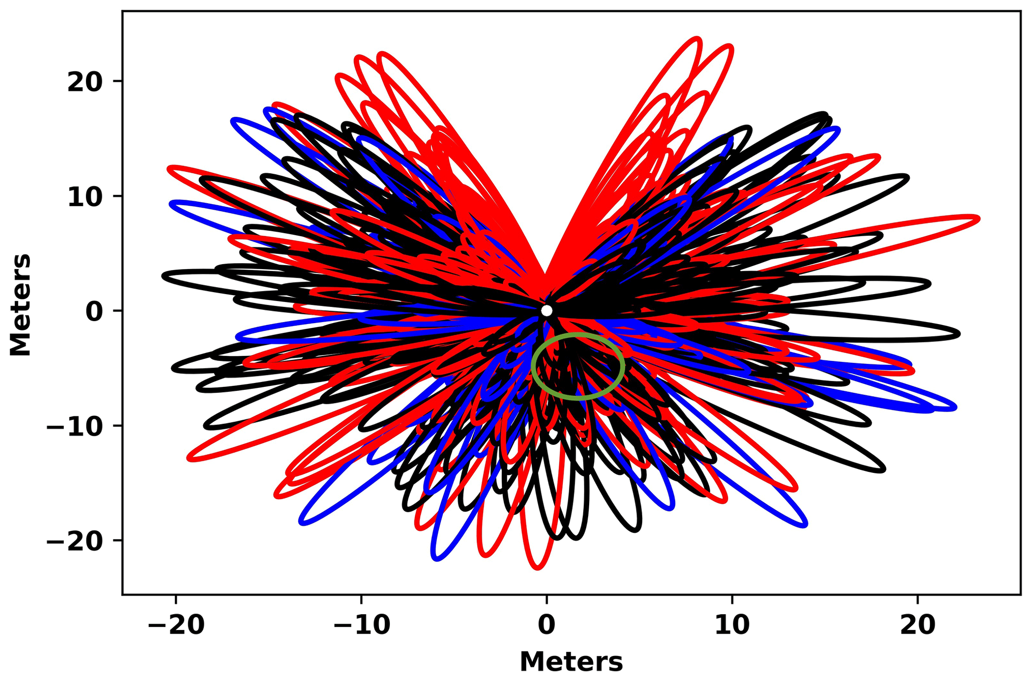
Figure 2 GNSS Fresnel ellipses around the geodetic antenna during one of the observation days. GPS constellations satellites are shown in black, GLONASS satellites are shown in red, and GALILEO satellites are shown in blue. The green circle is the location where the soil samples have been taken.

Therefore, the first novelty of this research was to extend, compare, and combine the GPS-IR methodology to a multi-constellation scenario (GPS, GLONASS, and GALILEO; BEIDU is not introduced in this research because the antennas used in the experiment are not able to decode BEIDU signals), which will produce a much larger sample set of observations around the antenna than is obtained with only the GPS constellation (as shown in Fig. 2).

Additionally, geodetic-quality GNSS receivers and antennas are an expensive solution. If we keep in mind that the final market will be the agricultural market, a technique developed using those devices will never be introduced into the sector. Thus, the (main) second novelty of this research was the introduction of mass-market GNSS sensors as the basis of the technique. If the use of these mass-market devices can be confirmed, it will be possible to use them (one or several at the same time to add redundancies) at a very low cost.

2 Materials and methods

2.1 Location of the experiment

The experiment was conducted in the installations of the Cajamar Centre of Experiences, located in Paiporta, Valencia, Spain (39^∘25^′3^′′ N, 0^∘25^′4^′′ W), which is an agricultural research technology centre (https://www.fundacioncajamarvalencia.es/es/comun/actividades/, last access: 20 February 2020, available in Spanish).

The centre began its activities in 1994. Some of the research topics carried out by the centre are the valorisation of agricultural by-products and the use of microorganisms in food, pharmaceuticals, and aesthetics using the latest biotechnology resources; the design of new containers and bio-functional formats for the marketing of healthy foods with high added value; the improvement in irrigation automation, biological control management, and agronomic management in organic production; and the introduction of alternative value crops and new varieties that guarantee the sustainability of the agricultural sector.

2.2 Instruments and observations

A geodetic GNSS receiver (Trimble R10 GNSS receiver from the Department of Cartographic Engineering Geodesy and Photogrammetry of the Universitat Politècnica de València) and a mass-market receiver (Navilock GNSS receiver based on a u-blox 8 UBX-M8030-KT chipset with a built-in antenna) connected to a Raspberry Pi 3, as a control device and for storing the observations, were used to obtain multi-constellation SNR observables (GPS, GLONASS, and GALILEO). A series of 5 s sample rate observations were obtained simultaneously for both sensors (Fig. 3).

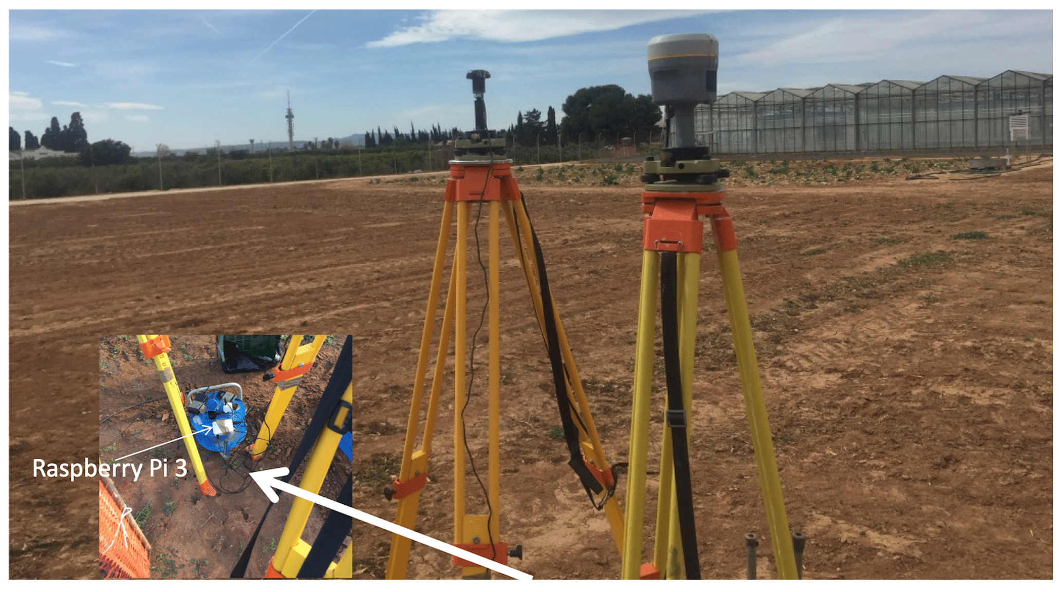
Figure 3 Instrumental configuration in the field campaign. A geodetic-quality GNSS antenna and a mass-market GNSS antenna were working at the same time.

The radio signal structure of GPS, GLONASS, and GALILEO systems are similar. Different carrier signals in the L band are broadcast, and L1 and L2 correspond with the two main frequencies of the signal emitted from the GPS satellites and E1 and E5, with the two main frequencies of the signal emitted from the GALILEO satellites. In contrast to GPS and GALILEO, GLONASS satellites transmit carrier signals at different frequencies from a basic L frequency. GLONASS L1 frequencies are as follows:

$$\begin{array}{}\text{(1)}& f_{\mathrm{L}\mathrm{1}}=f_{\mathrm{O}}+k\times \mathrm{\Delta }{f}_{\mathrm{L}\mathrm{1}}k=\mathrm{1},\mathrm{2},\mathrm{\dots }\mathrm{24},\end{array}$$

where f_O=1602.0 MHz, Δf_L1=0.5625 MHz, and k is the carrier number assigned to the specific GLONASS satellite (Hofmann-Wellenhof et al., 2008). Thus, the frequency for each satellite should be computed and included in the GLONASS file.

The frequencies used in the experiment were L1, for the GPS and GLONASS satellite constellations, and E1, for the GALILEO constellation. This choice was forced because the mass-market device could not track the L2 or E5 satellite signals. However, Vey et al. (2016) showed that the soil moisture root mean square difference between L2C and L1 was only 0.03 m³ m⁻³. L2C corresponds to the L2 civil signal of the block satellites IIR-M and IIF of the GPS constellation, which has only been available since 2005 when the first block IIR-M was launched. This signal is designed specifically to meet commercial needs, which increases robustness of the signal, improves resistance to interference, and improves accuracy (Leick et al., 2015).

The GNSS-IR footprint for a single rising or setting satellite is an elongated ellipse in the direction of the satellite track (Fresnel ellipse or zones; Larson et al., 2010; Wan et al., 2015; Vey et al., 2016; Roesler and Larson, 2018). As the satellite rises and the elevation angle increases, the Fresnel zone becomes smaller and closer to the GNSS antenna. Data with elevation angles higher than 30^∘ should be discarded from the SNR series because they contain no significant oscillations and cannot be retrieved reliably. Data with elevation angles lower than 5^∘ should also be discarded in order to avoid strong multipath effects from trees, artificial surfaces, and structures surrounding the antenna. A GNSS satellite takes about 1 h to rise from an elevation angle of 5^∘ to an angle of 30^∘.

The geodetic GNSS receiver store the observations (including SNR data) in the commonly used Receiver Independent Exchange Format (RINEX) files, so the elevation and azimuth of a satellite for an epoch should be computed from the observation RINEX file and the navigation RINEX file (Hofmann-Wellenhof et al., 2008).

The mass-market receiver uses the National Marine Electronics Association (NMEA) GSV sentences to provide integer numbers for elevation, azimuth, and signal-to-noise ratio (SNR) directly. The GNSS NMEA is a standard data format supported by all manufacturers to output measurement data from a sensor to a predefined format in ASCII. In the case of GNSS, it can output position, velocity, time, and satellite-related data (for the constellations that the antenna can decode). There are quite a few NMEA messages or sentences, specifically, and GSV sentences provide integer numbers for elevation, azimuth, and signal-to-noise ratio.

The results were compared to soil moisture measurements based on soil samples taken at a depth of 5 cm and weighed before and after being dried (gravimetric method) in a laboratory (Fig. 4). These measurements were considered to be the reference data set. One soil sample was taken per day, except over weekends, and the location, in comparison with the antenna position, can be seen in Fig. 2.

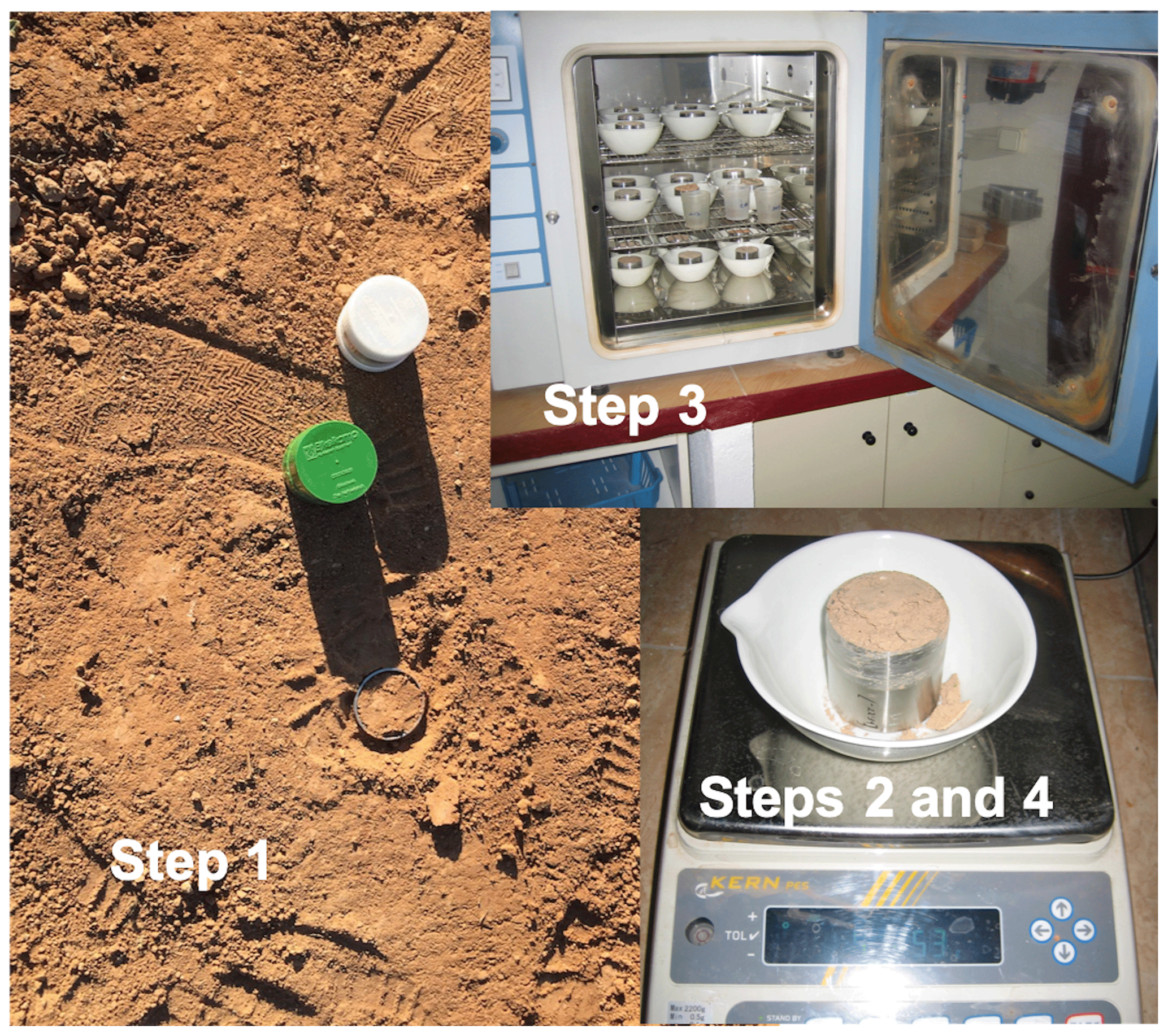
Figure 4 Gravimetry method used for producing a reference data set. Step 1: taking the soil sample. Steps 2 and 4: weighing the sample. Step 3: drying the sample.

In total, 66 d of measurements, from 3 December 2018 to 6 February 2019, were observed, processed, and analysed. The height of the antennas from the ground was 1.80 m for the geodetic GNSS device and 1.84 m for the mass-market device.

Precipitation data were added in the final plot results. These data were obtained from a meteorological station located in the Cajamar Experiences Centre (100 m from the GNSS antennas).

2.3 Theoretical background

The theoretical background is based on the procedure developed by Larson et al. (2010) and detailed in Chew et al. (2014), Vey et al. (2016), and Zhang et al. (2017). Each valid track of a satellite should be separated into the ascending path and descending path.

The processing of each satellite track can be summarised as follows:

1. SNR data are converted from dB units to linear scale in volts using the conversion equation (S stands for SNR in the next equation and for the rest of equations in the paper) $S_{\mathrm{lineal}}={\mathrm{10}}^{S/\mathrm{20}}$ (Vey et al., 2016).

2. A low-order polynomial (second degree) is fitted to the S_lineal in order to eliminate the direct satellite signal so that the reflected signal is isolated as follows: $S_{\mathrm{lineal}}^{\mathrm{reflected}}$ (Wan et al., 2015; Chew et al., 2016).

3. A Lomb–Scargle periodogram (Lomb, 1976; Press et al., 1992; Roesler and Larson, 2018) is then computed from $S_{\mathrm{lineal}}^{\mathrm{reflected}}$, and the track goes to the next step only if there is a clear signal that reflects a primary wave. Tracks with multiple peaks or low maximum average power (less than 4 times the background noise) are not included in the next step. If the Lomb–Scargle periodogram is computed using the sine elevation angle as the input x axis, the result converts the frequency into antenna height in the output x axis. Only tracks with computed antenna height consistent with the measured antenna height (less than 0.1 m difference) go to the next step.

4. The selected tracks are modelled using the following expression:

   $$\begin{array}{}\text{(2)}& S_{\mathrm{lineal}}^{\mathrm{reflected}}=A\cos \left({\displaystyle \frac{\mathrm{4}\mathit{\pi }h}{\mathit{\lambda }}}\sin e+\mathit{\phi }\right).\end{array}$$

   The equation means that $S_{\mathrm{lineal}}^{\mathrm{reflected}}$ can be modelled in terms of the amplitude A and phase offset φ of a primary wave. λ is the GNSS wavelength (L1 for GPS and GLONASS and E1 for GALILEO), e is the satellite elevation, and h is the antenna height, which is assumed to be a constant due to the low signal penetration on the ground (Chew et al., 2014; Roussel et al., 2016; Zhang et al., 2017). The least squares algorithm (Strang and Borre, 1997; Leick et al., 2015) is used to estimate A and φ.

5. Chew et al. (2014) derived a linear relationship between the previously computed phase offset and soil moisture, with a slope of 65.1^∘, in order to obtain the GNSS-derived volumetric water content (VWC), VWG_GNSS (m³ m⁻³). V stands for VWG_GNSS in the next equation and for the rest of the paper, as follows:

   $$\begin{array}{}\text{(3)}& V_{\mathrm{GNSS}}={\displaystyle \frac{\mathrm{\Delta }{\mathit{\phi }}_{\mathrm{t}}}{\mathrm{65.1}}}+V_{\mathrm{Residual}}.\end{array}$$

   However, this value should be computed using the reference values in order to convert the satellite tracks phase values into GNSS-derived volumetric water content because this linear relationship can be positive or negative. Zhang et al. (2017) showed the importance of this adjustment with the test data in order to obtain better results (their results showed a decrease in the final standard deviation from 0.036 m³ m⁻³ – using the linear relationship of 65.1^∘ – to 0.008 m³ m⁻³ – using the adjusted linear relationship).

   V_Residual in Eq. (3) is the minimum soil moisture observation from the reference data set (obtained from the soil samples). This minimum value should be taken from the reference observations as long as the GNSS observation is continuous and without interruptions. In the case that there is any interruption in the GNSS observation data, this value must be chosen again from the reference values after the interruption. $\mathrm{\Delta }{\mathit{\phi }}_{\mathrm{t}}=\mathit{\phi }-{\mathit{\phi }}_{\mathrm{o}}$ is calculated with respect to a reference phase φ_o computed in this work, as proposed by Chew et al. (2016) as follows: the mean of the lowest 15 % of the computed phases for each satellite track during the retrieval period. φ_o should be computed again in the case of an interruption of the GNSS signal, and ascending and descending paths for the same satellite are treated separately.

6. Finally, the mean V value of all satellite tracks from the same constellation that pass at different times during the day is computed, so that the final GNSS soil moisture represents a temporal average for all observations analysed during 1 d. To address the objectives of this research, we have three different results, namely one for each GNSS constellation.

3 Results

3.1 Processing

RINEX observation and navigation files from the geodetic GNSS antenna were used to generate the input file for the processing process. This file contained the year, month, day, hour, satellite identification, SNR, elevation, and azimuth for every observed epoch. We computed three different files (GPS, GALILEO, and GLONASS). The frequency for each GLONASS satellite should be also computed and included in the GLONASS file.

The file containing the NMEA observations from the mass-market antenna was used to generate three different input files for the processing process, namely one for each satellite constellation. However, due to the integer nature of the SNR, elevation, and azimuth observation numbers, an extra processing step was included for the mass-market observation files. This step used the navigation files from the International GNSS Service (IGS) repository (http://www.igs.org, last access: 1 March 2020) to compute float numbers for elevation and azimuth values of the observed satellites.

The rest of the processing followed the steps defined in the previous section. Only full GNSS track data, covering more than 30 min and covering more than 10^∘ of elevation in the trajectory, were considered in our study.

3.2 Results

The geodetic antenna SNR data, in volts for satellite GPS no. 23, are shown in Fig. 5a, the SNR data with the direct signal removed are shown in Fig. 5b, the Lomb–Scargle periodogram for the SNR-reflected signal is shown in Fig. 5c, and the SNR-reflected signal with the adjusted wave (Step 4 in the previous section) is shown in Fig. 5d. Figure 6 shows the same concepts for the same satellite but uses the mass-market antenna observations. Figures 7 and 8 show the same concepts for the GLONASS satellite no. 5, and Figs. 9 and 10 show these for the GALILEO satellite no. 21.

Figure 5 GPS satellite no. 23 observed with the geodetic antenna. SNR data in volts (a), SNR data with the direct signal removed (b), Lomb–Scargle periodogram for the SNR reflected signal (c), and SNR reflected signal with the adjusted wave (d).

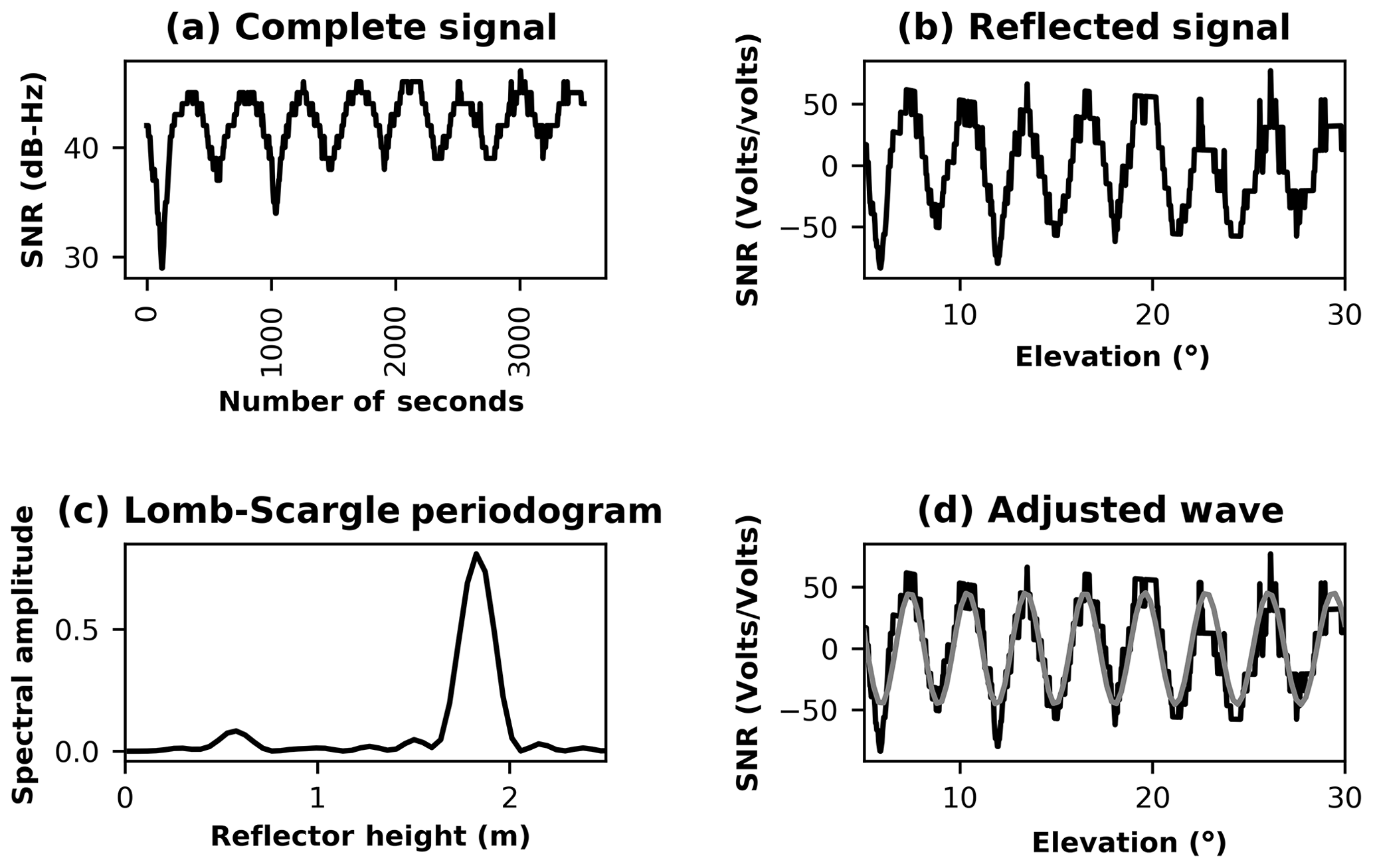
Figure 6 GPS satellite no. 23 observed with the mass-market antenna. SNR data in volts (a), SNR data with the direct signal removed (b), Lomb–Scargle periodogram for the SNR reflected signal (c), and SNR reflected signal with the adjusted wave (d).

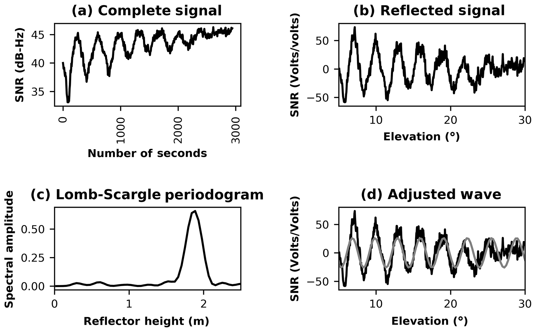
Figure 7 GLONASS satellite no. 5 observed with the geodetic antenna. SNR data in volts (a), SNR data with the direct signal removed (b), Lomb–Scargle periodogram for the SNR reflected signal (c), and SNR reflected signal with the adjusted wave (d).

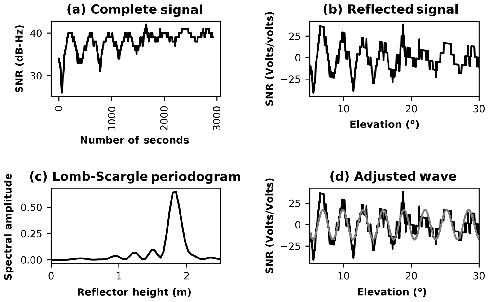
Figure 8 GLONASS satellite no. 5 observed with the mass-market antenna. SNR data in volts (a), SNR data with the direct signal removed (b), Lomb–Scargle periodogram for the SNR reflected signal (c), and SNR reflected signal with the adjusted wave (d).

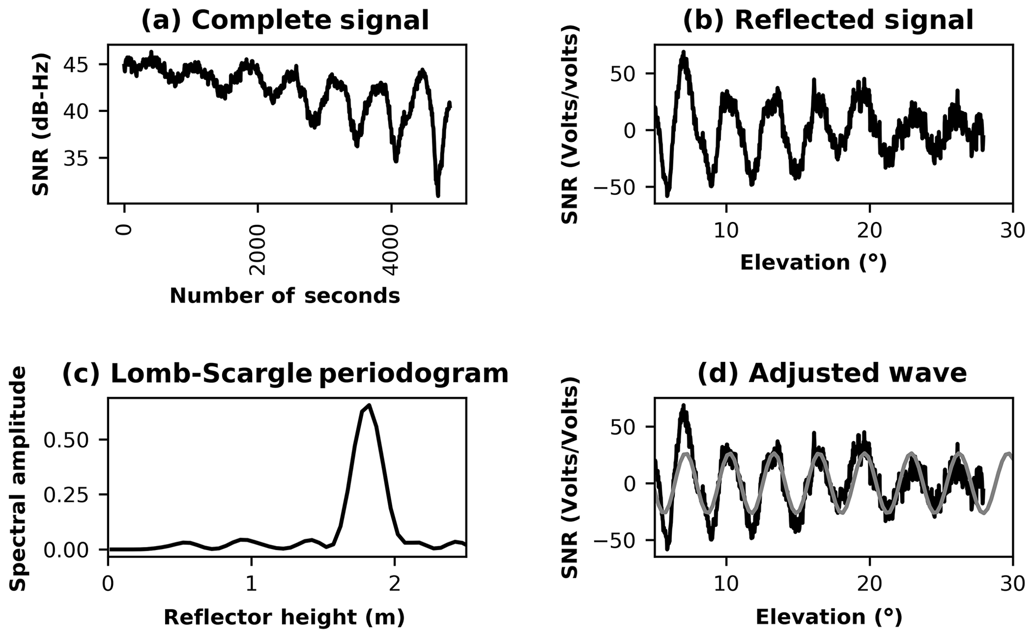
Figure 9 GALILEO satellite no. 21 observed with the geodetic antenna. SNR data in volts (a), SNR data with the direct signal removed (b), Lomb–Scargle periodogram for the SNR reflected signal (c), and SNR reflected signal with the adjusted wave (d).

Figure 10 GALILEO satellite no. 21 observed with the mass-market antenna. SNR data in volts (a), SNR data with the direct signal removed (b), Lomb–Scargle periodogram for the SNR reflected signal (c), and SNR reflected signal with the adjusted wave (d).

The SNR values from the geodetic antenna and the mass-market antenna for the GPS constellation are similar, as suggested by Li and Geng (2019), because the u-blox chipset uses an active, right-hand, circularly polarised antenna with uniform antenna gain. However, the SNR values for GLONASS and GALILEO present a systematic bias of about 3–5 dB-Hz between the geodetic and mass-market antennas (Figs. 7a, 8a, 9a, and 10a).

A linear relationship between the reference data and every GNSS constellation and antenna was computed using the methodology proposed by Zhang et al. (2017; the results can be seen in Table 1). Based on the positive values for all lineal relationships and the conclusions in Zhang et al. (2017), a slope of 65.1^∘ between the all-GNSS computed phase offset and the soil moisture was used to homogenise the results among the different constellations and the two different antennas.

Table 1 Linear relationship (in degrees) between GNSS observations and reference soil moisture observations.

However, two different values for V_Residual and φ_o were used due to an outage of the electrical power during 3 d (from day 40 to day 42 of the experiment), during which time no observations were recorded.

The results presented the average value of soil moisture around the geodetic and mass-market antennas per day, as obtained from all valid GNSS tracks of all satellites per constellation or from using the three constellations.

Figures 11–13 show a comparison of the daily soil moisture from GPS, GLONASS, and GALILEO, respectively, where the results of the geodetic and mass-market antennas can be compared to the reference gravimetric data set. Daily precipitation amounts are also included in the figures.

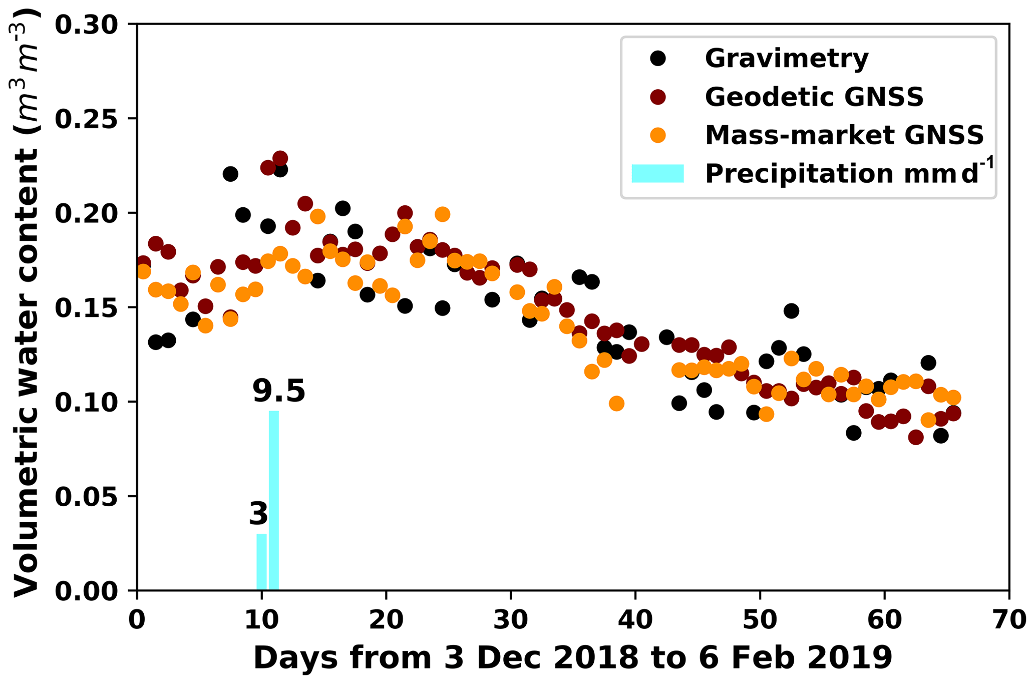
Figure 11 GPS comparison of daily soil moisture. The results of the geodetic and mass-market antennas are compared with the reference gravimetric data set.

Figure 12 GLONASS comparison of daily soil moisture. The results of the geodetic and mass-market antennas are compared with the reference gravimetric data set.

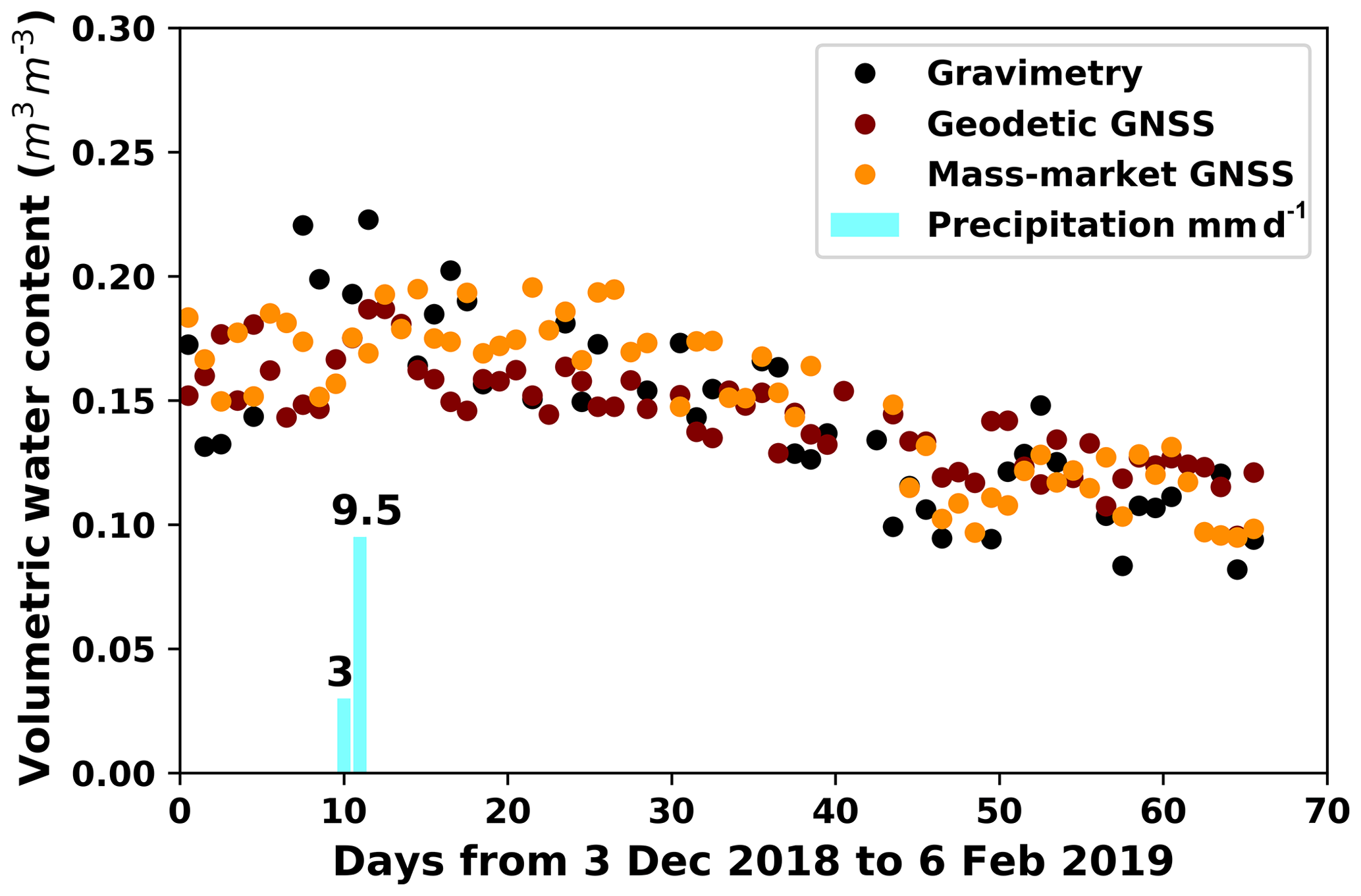
Figure 13 GALILEO comparison of daily soil moisture. The results of the geodetic and mass-market antennas are compared with the reference gravimetric data set.

Finally, Fig. 14 shows the combined solution of the three constellations as an average of the results of the individual solutions, which can be considered a combined multi-constellation solution.

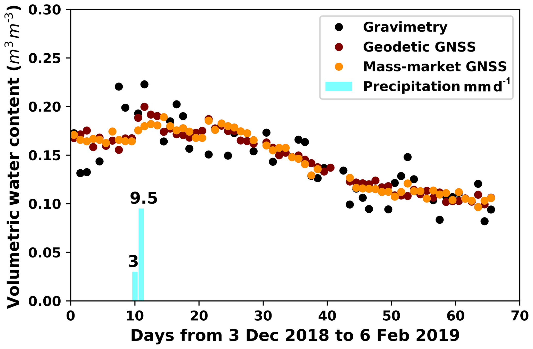
Figure 14 Multi-constellations GNSS (GPS–GLONASS–GALILEO combination) comparison of daily soil moisture. The results of the geodetic and mass-market antennas are compared with the reference gravimetric data set.

Table 2 Statistical summary of the soil moisture estimates from the GPS, GALILEO, and GLONASS constellations with the reference (in situ) values. GNSS is the combination of the three constellations. RMSE is the root mean square error, MAE is the mean absolute error, and SD is the standard deviation of the differences.

The numerical values for Figs. 11–14 are listed in Table 2, where MAE is the mean absolute error, RMSE is the root mean square error, and mean and SD are the mean and the standard deviation, respectively, between the GNSS antennas and the reference values. The Pearson correlation coefficient can be used to summarise the strength of the linear relationship between two data samples. The Spearman correlation can be used to summarise whether two variables are related with a non-linear relationship and whether that the relationship is stronger or weaker across the distribution of the variables.

4 Discussion

Based on the results summarised in Table 2, equivalent results between geodetic and mass-market antenna are obtained for RMSE, MAE, mean, and SD, showing the good performance of the mass-market antenna. The Pearson and Spearman correlations are equivalent between geodesic and mass-market antenna for every constellation and for comparing the constellations. These confirm that a lineal relationship can be considered between the soil moisture results obtained from all GNSS antennas and the sample observations.

The least favourable results in terms of RMSE, MAE, and SD were obtained for the GALILEO constellation; one of the possible causes is that it does not have as many satellites in the constellation as the GPS and GLONASS constellations do. The GLONASS constellation offers slight improvements in terms of RMSE, MAE, and SD results in comparison with GPS. The GLONASS range of values appears more compressed for both the geodetic and mass-market antennas; one of the possible causes is that GPS constellation, at the moment of the observations, had three different satellite blocks (namely, blocks IIR, IIF, and IIF) with different capabilities and GLONASS had only two (namely, blocks M and K). However, the ranges of RMSE, MAE, and SD, when considering GPS, GLONASS, and GALILEO constellations (both geodetic and mass-market antennas), are less than 0.01 m³ m⁻³ and less than 0.15 for the Pearson or Spearman correlations, so we can consider that the three constellations produce similar V_GNSS values, regardless of the type of antenna used, opening the possibility of using the three constellations, in combination, as a multi-constellation solution. The last two columns of Table 2 show the statistical summary of the constellations combination for both the geodetic and the mass-market antenna, where it can be seen that the values obtained are equivalent to those in the previous columns.

Our RMS results, using the a priori slope values of 65.1^∘, are comparable with those obtained by Zhang et al. (2017), who processed 6 months of continuous observations and obtained a mean standard deviation value of 0.036 m³ m⁻³, and those of Vey et al. (2016), who processed 6 years of observations and obtained a standard deviation value of 0.06 m³ m⁻³.

The SNR bias between the geodetic and mass-market antenna for GLONASS and GALILEO constellations (Figs. 7b, 8b, 9b, and 10b) has no effect in the final phase offset variations for the adjusted wave.

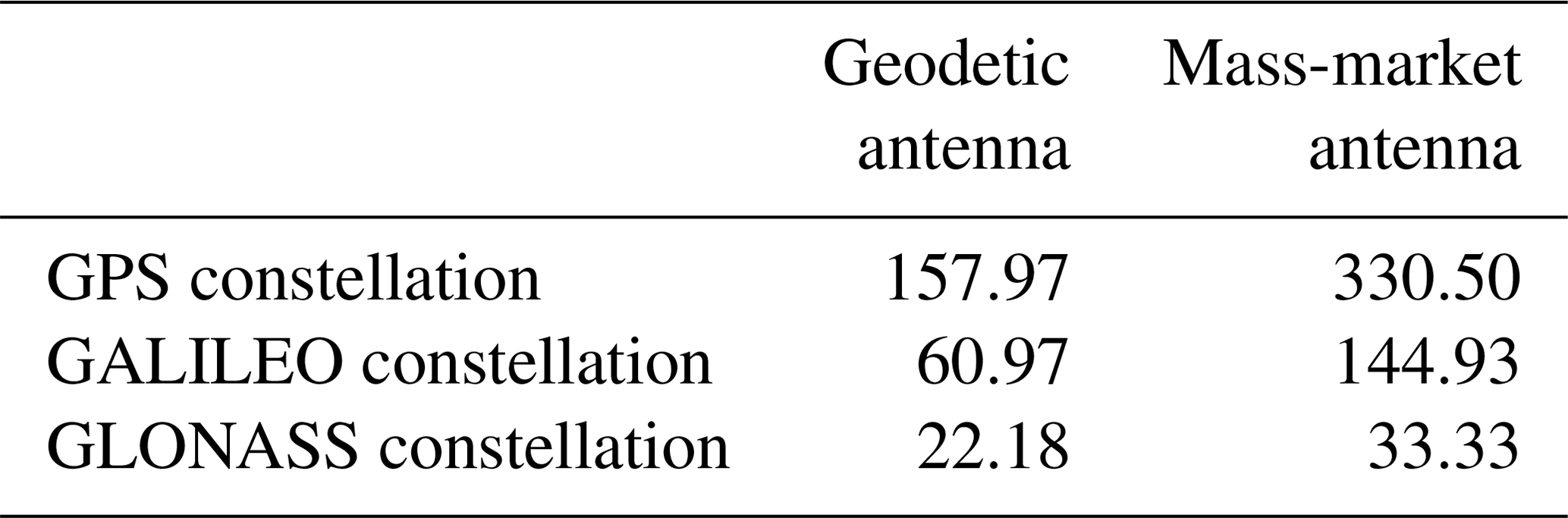
According to Step 3 of Sect. 2.3, 70 % of the GPS tracks recorded by the geodetic antenna were considered valid for processing, as were 73 % for GALILEO and 74 % for GLONASS. This percentage is reduced to around a 10 % if we consider the tracks recorded by the mass-market antenna. Nonetheless, one of the main important problems in this research is related to the selection of the correct tracks to be processed and adjusted using Step 4 of Sect. 2.3. Based on the mentioned criteria (tracks with multiple peaks or low maximum average power and computed reflector height consistent with the measured antenna height), some tracks that should not be processed are finally processed (around 8 % of all tracks irrespective the constellation). These wrongly processed tracks introduce outliers in the computed V_GNSS, which are eliminated in the daily final mean V_GNSS computation because they produce a high RMS in the daily computations using all satellites. One way to accomplish this task could be to use good figures, such as those in Fig. 5c–d, to produce a valid set of training images and use machine-learning tools (image recognition) to decide automatically whether a new track can be considered to be a good track (so it can be processed) or not. This idea is currently under development.

In situ observations are needed to solve Eq. (3; V_Residual parameter). However, if there are no reference values, this constant cannot be included, and the results will present an offset in comparison with the real values. A possible solution would be the estimation of the parameter based on the soil type (URL 1); though, that requires having a long enough time series to make the assumption that, at some point during the time series, soil moisture was low enough to hit the residual value. However, the results can be used in a relative way; that is, they can be used to infer VWC variations from 1 d to another. This relative comparison can be performed only if the observations are continuous. If there is an interruption in the raw data (because the antenna is turned off) of more than 2 or 3 h, the previous reference is lost and the relative comparisons should start again (from the moment the antenna is turned on again). In situ observations are also needed if we want to adjust the linear relationship between the computed phase offset and the soil moisture, as is developed in Zhang et al. (2017); however, in case the linear relationship is positive, a value of 65.1^∘ can also be used to obtain acceptable results.

5 Conclusions

The case study presented in this research is focused on the GNSS SNR data acquisition and processing using the GNSS-IR technique to monitor soil moisture. The main objectives of this research were the use, comparison and combination of GPS, GLONASS, and GALILEO constellations solutions and the use and comparison of geodetic and mass-market antenna solutions.

Independent GPS, GLONASS, and GALILEO solutions were generated to demonstrate that the technique can be extended to a multi-constellation solution. This is necessary because a single constellation solution presents a reflection footprint that is far from homogeneous around the antenna and because 30 %–35 % of the observed satellite tracks of the geodetic antenna are not valid for processing (40 %–45 % if the mass-market antenna is considered).

The use of a mass-market GNSS antenna was confirmed to be a viable tool for GNSS-IR, with the caution of using the IGS navigation files to transform the observed integer numbers obtained in the NMEA messages for the elevation and azimuth of the satellites into floating numbers. With the use of mass-market sensors, it will become possible to design scenarios with several GNSS stations generating redundant observations. Therefore, maps of soil moisture variations according to specific and selective areas of soil, cultivation, and/or management can be generated instead of obtaining only an average value for the entire observation area.

GNSS-IR is still a technique with numerous technological challenges in order to become a competitive solution with respect to current observation techniques, but it has great potential with regards to the continuity of observation (it can be implemented in a real or quasi-real time scenario), precision, and measurement acquisition cost if mass-market antennas are used.