Sensitivity of meteorological-forcing resolution on hydrologic variables

Projecting the spatiotemporal changes in water resources under a no-analog future climate requires physically based integrated hydrologic models which simulate the transfer of water and energy across the earth's surface. These models show promise in the context of unprecedented climate extremes given their reliance on the underlying physics of the system as opposed to empirical relationships. However, these techniques are plagued by several sources of uncertainty, including the inaccuracy of input datasets such as meteorological forcing. These datasets, usually derived from climate models or satellite-based products, are typically only resolved on the order of tens to hundreds of kilometers, while hydrologic variables of interest (e.g., discharge and groundwater levels) require a resolution at much smaller scales. In this work, a high-resolution hydrologic model is forced with various resolutions of meteorological forcing (0.5 to 40.5 km) generated by a dynamical downscaling analysis from the regional climate model Weather Research and Forecasting (WRF). The Cosumnes watershed, which spans the Sierra Nevada and Central Valley interface of California (USA), exhibits semi-natural flow conditions due to its rare undammed river basin and is used here as a test bed to illustrate potential impacts of various resolutions of meteorological forcing on snow accumulation and snowmelt, surface runoff, infiltration, evapotranspiration, and groundwater levels. Results show that the errors in spatial distribution patterns impact land surface processes and can be delayed in time. Localized biases in groundwater levels can be as large as 5–10 m and 3 m in surface water. Most hydrologic variables reveal that biases are seasonally and spatially dependent, which can have serious implications for model calibration and ultimately water management decisions.

1 Introduction

Understanding water and energy fluxes across the earth's critical zone, a region spanning from bedrock to vegetation canopy, is important to assess the impacts of climate change on water resources. Integrated hydrologic models, solving water–energy interactions and transfers, across the lower atmosphere, the land surface, and the subsurface, allow for analyzing water resources in both time and space and projecting into a no-analog future where empirical models are no longer valid. With the advancement of computing power, these high-fidelity, high-resolution models are becoming widely used (e.g., MIKE-SHE of Abbott et al., 1986, HydroGeoSphere of Panday and Huyakorn, 2004; and ParFlow-CLM – Community Land Model – of Maxwell and Miller, 2005). However, their implementation can be plagued by several sources of uncertainty. While the accuracy, the precision, and the uncertainty reduction of hydrologic models are extensively discussed in the literature, more attention is given to the physical representation of the phenomena occurring in the hydrological systems (Beven, 1993; Beven and Binley, 1992; Liu and Gupta, 2007), the reduction of uncertainties related to the hydrodynamic parameters (Gilbert et al., 2016; Janetti et al., 2019; Maina and Guadagnini, 2018; Srivastava et al., 2014), and the numerical resolution of the mathematical equations governing the physics of the environment (Belfort et al., 2009; Bergamaschi and Putti, 1999; Fahs et al., 2009; Hassane Maina and Ackerer, 2017; Miller et al., 1998; Tocci et al., 1997).

Atmospheric dynamics (e.g., precipitation patterns) constitute one of the main drivers of the simulated hydrologic processes. Unfortunately, measuring atmospheric conditions is difficult and is often only at point locations with stations which are difficult to maintain. Thus, models relying on data assimilation methods that fuse observations at different scales and remote sensing products are commonly used to generate the spatiotemporal distribution of meteorological variables. Furthermore, because integrated hydrologic models require many meteorological variables (i.e., precipitation, temperature, wind speed, solar radiation, air pressure, and relative humidity), synthetic data from climate models are often used due to the scarcity of measurements. In addition, in the context of climate change, only climate models can provide a spatial distribution of meteorological conditions. Also, integrated hydrologic models require high-resolution forcing to ensure fidelity and accuracy, and meteorological variables such as precipitation, one of the most important data and key control of hydrological models, are very heterogeneous especially in mountainous areas (Olsson et al., 2014; Prein et al., 2013).

Like any model input, meteorological forcing is impacted by several sources of uncertainty, including the fidelity of the physics of the atmospheric model as well as the representativity of the spatial resolution at which they occur. The impact of precipitation resolution on runoff and streamflow is widely documented in the literature with studies relying on (i) empirical hydrologic models with precipitation data coming from measurements (Arnaud et al., 2002; Berne et al., 2004; Lobligeois et al., 2014; Nicótina et al., 2008; Schilling, 1991; Shrestha et al., 2006; Tobin et al., 2011), satellite-based products (Koren et al., 1999; Ochoa-Rodriguez et al., 2015; Vergara et al., 2013), and climate model outputs (Dankers et al., 2007; Kleinn et al., 2005) and (ii) physics-based hydrologic models with precipitation data coming from measurements (Elsner et al., 2014; Fu et al., 2011), satellite-based products (Eum et al., 2014; Haddeland et al., 2006), and climate model outputs (Mendoza et al., 2016; Rasmussen et al., 2011). Moreover, Rasmussen et al. (2011) study the impact of meteorological forcing on snow dynamics.

Nevertheless, previous studies were mostly focused on runoff and streamflow analysis, lacking a complete analysis of all the hydrodynamic processes occurring at the watershed scale. Moreover, the resolutions of the meteorological data (km) used remain relatively coarse compared to the scale of resolution of the hydrological models (m). Hence, the objective of this study is to investigate the impact of the spatial resolution of the meteorological forcing from kilometers to meters on the hydrologic processes occurring at the watershed scale using a physics-based integrated hydrologic model. In other words, we seek to understand how the uncertainties associated with the coarse spatial resolution of meteorological forcing propagate into the high-resolution integrated hydrologic models and affect the output of interest.

While in this study we utilize specific models to quantify the impact of meteorological forcing on hydrologic variables, the results generalized for watershed processes and are meant to be illustrative of the potential bias with various codes and in various locations. In this work, we use ParFlow-CLM (Kollet and Maxwell, 2006; Maxwell, 2013; Maxwell and Miller, 2005) forced with the Weather Research and Forecasting (WRF) model (Skamarock et al., 2008; Skamarock and Klemp, 2008). ParFlow simulates subsurface and surface flows (as well as their interaction) by solving the mixed form of the Richards equation (Richards, 1931) and the kinematic-wave equation, respectively. The transfer of water and energy from the subsurface and the land surface to the atmosphere is simulated using a coupled version of the Community Land Model (CLM; Dai et al., 2003) to ParFlow. Therefore, the model allows for the spatiotemporal analysis of all the hydrological components of interest such as the distribution of pressure head, which encompasses the information on the water level in the river and the groundwater, the groundwater and surface water storages, the evapotranspiration, the infiltration, and the snow dynamics. WRF is a state-of-the-art, fully compressible, nonhydrostatic, mesoscale numerical weather prediction model that simulates the physics governing the atmospheric dynamics using a nested-domain configuration to provide meteorological-forcing data at different spatial resolutions for ParFlow-CLM.

Our study focuses on the Cosumnes watershed located in northern California, USA, a region where the effects of climate change have already been observed. The latter are characterized by a fluctuation between extreme droughts (Griffin and Anchukaitis, 2014) and the subsequent occurrence of unprecedented wildfires and periods of intense precipitation mainly caused by atmospheric rivers (Dettinger, 2011). Atmospheric rivers, filaments of concentrated moisture in the atmosphere, generate storms with intensity much higher than the average precipitation events and are sometimes very localized. The Cosumnes hosts one of the last rivers without a dam in California, offering the opportunity to study natural flow. The watershed also spans the Sierra Nevada–Central Valley interface, offering an opportunity to assess the relationship between snowpack dynamics, large-scale river runoff, and aquifer storage. The region is representative of many watersheds in the state, given the strong variations in topography and land cover and land use, but also the snow dynamics, given that the majority of the water resources in the state originate from snowmelt (Dettinger and Anderson, 2015). These sharp variations in above- and belowground heterogeneities necessitate high-resolution models, making it an excellent candidate to understand the impact of the forcing resolution on hydrology.

We study the water year (WY) 2017, the wettest water year on California record characterized by several atmospheric rivers (Di Liberto, 2017; SCRIPPS Institution of Oceanography, 2017). As mentioned by Swain et al. (2018), the future climate of California will likely be characterized by extreme wet and dry conditions. It is therefore important to understand the dynamics of these currently end-member conditions. Although exceptional today, these extremes will likely become the “new normal” in the future. Wet conditions are also ideal to conservatively understand the amount of bias an overly coarse meteorological-forcing dataset might have on a region's hydrology. The developed integrated hydrologic model has a spatial resolution of 200 m, and we use five different spatial resolutions (40.5, 13.5, 4.5, 1.5, and 0.5 km) of meteorological forcing derived from the WRF dynamical downscaling approach. Our study aims to answer the following questions:

• What is the effect of meteorological-forcing spatial resolution on simulated snow accumulation and melt, evapotranspiration, infiltration and pressure head, and/or water table depth? In broader terms, how do meteorological uncertainties propagate into the resolved hydrodynamics, and which processes require high-resolution meteorological forcing?

• At which spatial resolution should the climate models be solved to accurately describe the strong variations in meteorological conditions induced by atmospheric rivers and their effect on the hydrology and therefore water supply?

2 The Cosumnes watershed model

Study area

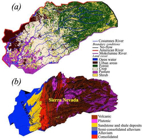
The Cosumnes watershed is approximately 7000 km² in size (Fig. 1a) and hosts one of the last rivers in the region without a major dam. Thus, it offers a rare opportunity to study the natural flow conditions. The geologic composition consists of materials ranging from nearly impermeable formations (volcanic and plutonic rocks located mainly in the Sierra Nevada Mountains) to highly porous and permeable aquifers in the Central Valley. The agricultural region of the Central Valley, subject to seasonal pumping and irrigation, is located in the southwest of the watershed and consists of various crop types, including alfalfa, pasture lands, and vineyards. The Sierra Nevada Mountains are predominately covered by an evergreen forest. Spatial patterns of precipitation are highly heterogeneous across the watershed. On average, the Sierra Nevada Mountains receive 3 times more precipitation (1500 mm) than the Central Valley (Cosgrove et al., 2003), primarily in the form of snow. The regional climate is considered Mediterranean, with wet and cold winters (with a watershed average temperature equal to 0 ^∘C) and hot and dry summers (with watershed average temperature reaching 25 ^∘C) (Cosgrove et al., 2003).

Figure 1 (a) Land use and land cover (Homer et al., 2015) and (b) geology (Jennings et al., 1977) and topography (United States Geological Survey, USGS) of the Cosumnes watershed.

3 Numerical-modeling methods

In this section, we briefly describe the two numerical models that we used in this study: (1) ParFlow-CLM, which simulates interactions as well as the transfer of water and energy between the lower atmosphere, the land surface, and the subsurface, and (2) Weather Research Forecast (WRF), which simulates mesoscale numerical weather prediction and is used here to drive the meteorological conditions of the ParFlow-CLM simulations.

3.1 Integrated hydrologic model: ParFlow-CLM

ParFlow-CLM (Kollet and Maxwell, 2006; Maxwell, 2013; Maxwell and Miller, 2005) describes the movement of water in the subsurface by solving the three-dimensional mixed form of Richards equation (Richards, 1931) given by

$$\begin{array}{}\text{(1)}& \begin{array}{rl}{S}_{\mathrm{S}}{S}_{\mathrm{W}}\left({\mathit{\psi }}_{\mathrm{P}}\right){\displaystyle \frac{\partial {\mathit{\psi }}_{\mathrm{P}}}{\partial t}}& +\mathit{\varphi }{\displaystyle \frac{\partial S_{\mathrm{W}}\left({\mathit{\psi }}_{\mathrm{P}}\right)}{\partial t}}\\ & =\mathrm{\nabla }\left[k\left(x\right)k_{\mathrm{r}}\left({\mathit{\psi }}_{\mathrm{P}}\right)\mathrm{\nabla }\left({\mathit{\psi }}_{\mathrm{P}}-z\right)\right]+q_{\mathrm{s}},\end{array}\end{array}$$

where S_S is the specific storage (L⁻¹), S_W(ψ_P) is the degree of saturation (–) associated with the subsurface pressure head ψ_P (L), t is the time, ϕ is the porosity (–), k_r is the relative permeability (–), z is the depth (L), q_s is the source–sink term (T⁻¹), and k(x) is the saturated hydraulic conductivity (L T⁻¹). The interdependence of variables (i.e., relationships between saturation and pressure head and between relative permeability and pressure head) is described by the van Genuchten model (van Genuchten, 1980). Overland flow is described by the two-dimensional form of the kinematic-wave equation given by

$$\begin{array}{}\text{(2)}& -k\left(x\right)k_{\mathrm{r}}\left({\mathit{\psi }}_{\mathrm{0}}\right)\mathrm{\nabla }\left({\mathit{\psi }}_{\mathrm{0}}-z\right)={\displaystyle \frac{\partial ∥{\mathit{\psi }}_{\mathrm{0}},\mathrm{0}∥}{\partial t}}-\mathrm{\nabla }\mathit{\upsilon }∥{\mathit{\psi }}_{\mathrm{0}},\mathrm{0}∥-q_{\mathrm{r}}\left(x\right),\end{array}$$

where ∥ψ₀,0∥ indicates the greater term between ψ₀ the surface pressure head and 0, υ is the depth-averaged velocity vector of surface runoff (L T⁻¹), and q_r represents rainfall and evaporative fluxes (L T⁻¹). The depth of the ponding water at the surface in the x direction (υ_x) and y direction (υ_y) is calculated by

$$\begin{array}{}\text{(3)}& {\mathit{\upsilon }}_x={\displaystyle \frac{\sqrt{S_{\mathrm{f},x}}}{n}}{\mathit{\psi }}_{\mathrm{0}}^{\mathrm{2}/\mathrm{3}}\mathrm{and}{\mathit{\upsilon }}_y={\displaystyle \frac{\sqrt{S_{\mathrm{f},y}}}{n}}{\mathit{\psi }}_{\mathrm{0}}^{\mathrm{2}/\mathrm{3}},\end{array}$$

where S_f,x and S_f,y are the friction slopes in the x and y directions (respectively) and n is the Manning coefficient.

Solutions of the Richards and kinematic-wave equations require the terms q_s and q_r(x), respectively. These terms include the land surface processes simulated by CLM, such as evapotranspiration, infiltration, and snow dynamics. To compute these processes, CLM uses soil moisture calculated by ParFlow, vegetation characteristics (the type of land use and land cover as well as its physical properties), and the meteorological forcing calculated by WRF.

The Cosumnes ParFlow-CLM model is horizontally resolved at 200 m and varies in vertical discretization from 10 cm at the land surface to 30 m at the bottom of the domain. The total thickness of the domain is 80 m. An analysis of variations in measured groundwater levels showed that this thickness is sufficient to capture water table depth fluctuations and that in general, beyond 50 m below the ground surface, the aquifer remains fully saturated. Simulations utilize parallel high-performance computing to accommodate the large number of cells (approximately 1.4 million) that constitute the high-resolution model.

The Cosumnes watershed is bounded by the American and Mokelumne rivers and is constrained in the model with the use of weekly varying values of Dirichlet boundary conditions along these borders. A no-flow (i.e., Neumann) boundary condition is imposed at the eastern, headwater side of the watershed. Hydrodynamic properties (including hydraulic conductivity, specific storage, porosity, and van Genuchten parameters) are derived from a regional geological map (Geologic Map of California, 2015; Jennings et al., 1977) and a literature review of previous studies (Faunt et al., 2010; Faunt and US Geological Survey, 2009; Flint et al., 2013; Gilbert and Maxwell, 2017; Welch and Allen, 2014). The 2011 National Land Cover Database (NLCD) map (Homer et al., 2015) is used in CLM to define land use and land cover. Agricultural maps provided by the National Agricultural Statistics Service (NASS) of the US Department of Agriculture's (USDA) Cropland Data Layer (CDL) (Boryan et al., 2011) are used to further delineate specific croplands in the Central Valley. Vegetation parameters are defined by the International Geosphere-Biosphere Programme (IGBP) database (IGBP, 2018). The developed model also accounts for pumping and irrigation occurring in the Central Valley. More details about the model parameterization and validation can be found in Maina et al. (2020) and Maina and Siirila-Woodburn (2020).

A full water year is simulated to demonstrate how different scales of meteorological forcing impact both wet and dry seasons of the year. The water year 2017 (i.e., 1 October 2016–30 September 2017), a particularly wet year, is selected to conservatively demonstrate how forcing scales may impact hydrologic results in a wide range of weather conditions.

3.2 Meteorological model: Weather Research Forecast (WRF)

WRF (Skamarock et al., 2008; Skamarock and Klemp, 2008) is a state-of-the-art, fully compressible, nonhydrostatic, mesoscale numerical weather prediction model. As shown in Fig. 2, we configure WRF version 3.6.1 over four two-way nested domains with a horizontal resolution of 13.5 km (domain d01), 4.5 km (domain d02), 1.5 km (domain d03), and 0.5 km (domain d04). Each domain is composed of 30 vertical atmospheric levels. Land cover in WRF matches the one used in ParFlow-CLM. Post-spin-up soil moisture from ParFlow-CLM is used to initialize the WRF model at the beginning of the simulation. Other WRF initial conditions, as well as boundary conditions, are defined based on the NLDAS-2 (North American Land Data Assimilation System; Cosgrove et al., 2003) terrestrial and meteorological data. The lateral boundary condition is specified for the coarse grid (d01 in Fig. 2) to constrain wind speed and direction, potential temperature, mixing ratio for water vapor, geopotential height, and hydrostatic pressure. The parametrizations that represent physical processes in the configuration of WRF used here include the Dudhia scheme (Dudhia, 1988) for shortwave radiation, the Rapid Radiative Transfer Model (Mlawer et al., 1997) for longwave radiation, the Morrison double-moment scheme (Morrison et al., 2009) for microphysics, the University of Washington Boundary Layer Scheme (Bretherton and Park, 2009) for the planetary boundary layer, and the Eta similarity scheme (Monin and Obukhov, 1954) for the model surface layer. The Grell–Freitas scheme (Grell and Freitas, 2014) is used for cumulus parameterization in two outermost domains only (d01 and d02). For domain d03 and d04, the higher resolutions allow for convection to be resolved explicitly. WRF mass balance validation results are shown in Appendix A1. The described configuration of WRF has been extensively validated against ground observation of meteorological conditions in the California region in previous works (Vahmani et al., 2019; Vahmani and Jones, 2017). These studies show a very good performance for the current configuration of WRF over California, predicting daily mean and maximum air temperatures and evapotranspiration with errors of 1.1 ^∘C, 0.4 ^∘C, and 0.74 mm d⁻¹, respectively. We further compare WRF simulations over the Cosumnes watershed with ground measurements (see Appendix A3). Our comparisons indicate a reasonable match between measurements and simulations, allowing us to gain confidence in the ability of WRF to reproduce the atmospheric dynamics in this watershed.

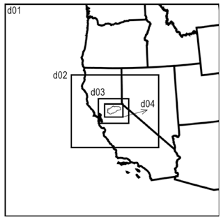
Figure 2 Geographical representation of four WRF nested domains with 13.5, 4.5, 1.5, and 0.5 km spatial resolutions for d01, d02, d03, and d04, respectively.

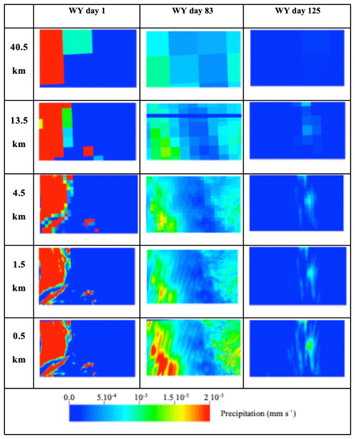
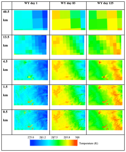
Using the nested-domain configuration of WRF described above, we design a series of simulations to dynamically downscale across the four spatial resolutions. The coarsest scale of forcing at 40.5 km resolution is generated by statistically upscaling the coarsest of the WRF simulations (13.5 km). WRF simulations are conducted from 1 September 2016 to 30 September 2017, covering the entire water year 2017 plus 1 month of spin-up. Spatial distributions of precipitation and temperature at three selected times (characterized by three different storms of varying intensity and duration) obtained with the five spatial resolutions of forcing are shown in Appendix A2.

3.3 Hydrologic variables

Results from the five spatial resolutions are compared for key land surface and subsurface processes. We consider the results obtained with the finest spatial resolution of meteorological forcing (0.5 km, closest to that of the hydrologic model) as the most accurate resolution and evaluate the differences relative to that of the four remaining resolutions (1.5, 4.5, 13.5, and 40.5 km). Comparisons are shown as an absolute error (AE) and/or percent error (PE) relative to the 0.5 km results via

$$\begin{array}{}\text{(4)}& {\mathrm{AE}}_{i,t}=X_{{\mathrm{0.5}}_{i,t}}-X_{R_{i,t}}\end{array}$$

and

$$\begin{array}{}\text{(5)}& {\mathrm{PE}}_{i,t}={\displaystyle \frac{X_{{\mathrm{0.5}}_{i,t}}-X_{R_{i,t}}}{X_{{\mathrm{0.5}}_{i,t}}}}\times \mathrm{100},\end{array}$$

where X is the model output (evapotranspiration – ET, infiltration – I, snow water equivalent – SWE, or ψ) at a given point in space (i) at a time (t) and R is the spatial resolution of the forcing (1.5, 4.5, 13.5, or 40.5 km). Snapshots in time of these errors highlight the sensitivity of each scale of forcing in space. Global (i.e., domain-wide) differences are also calculated for select parameters of interest and shown as a function of time.

Because large-scale changes in storage are of interest from a water management perspective, total surface water (SW) storage is calculated via

$$\begin{array}{}\text{(6)}& {\mathrm{Storage}}_{\mathrm{SW}}=\sum _{i=\mathrm{1}}^{n_{\mathrm{SW}}}\mathrm{\Delta }{x}_i\times \mathrm{\Delta }{y}_i\times {\mathit{\psi }}_i,\end{array}$$

where n_SW is the total number of river cells (–), Δx_i and Δy_i are cell discretizations along the x and y directions (L), and i indicates the cell. Similarly, total groundwater (GW) storage is calculated via

$$\begin{array}{}\text{(7)}& {\mathrm{Storage}}_{\mathrm{GW}}=\sum _{i=\mathrm{1}}^{n_{\mathrm{GW}}}\mathrm{\Delta }{x}_i\times \mathrm{\Delta }{y}_i\times \mathrm{\Delta }{z}_i\times {\mathit{\psi }}_i\times \left(S_{{\mathrm{s}}_i}/{\mathit{\varphi }}_i\right),\end{array}$$

where n_GW is the total number of subsurface saturated cells (–) and Δz_i is the discretization along the vertical direction the cell (L).

4 Results and discussions

4.1 Snow water equivalent (SWE)

Figure 3 shows the domain total SWE obtained with the five resolutions of forcing. Our results indicate that all four resolutions overestimate SWE when compared to the results obtained with 0.5 km forcing. We note that the accumulation of SWE starts at the same time for all resolutions, while the time of snowmelt peak varies considerably from one resolution to another; the coarser resolutions show a delay in ablation. For example, SWE results obtained with the 40.5 km resolution forcing exhibits low global error for the first half of the water year; however during peak ablation the differences are very large both in terms of magnitude (PE = 90 %) and timing (which is delayed by around 40 d). Our results show that an accurate representation of SWE requires forcing data with a resolution close to that of the hydrologic model. This conclusion is somewhat different from that drawn by Rasmussen et al. (2011), who found that the representation of SWE in mountainous systems can be accurate for spatial resolutions of forcing lower than 6 km. A possible explanation for this difference is the resolution of the physics-based model used in this study compared to that of Rasmussen and coauthors, the integrated hydrologic model we used in addition to the climate model, or differences stemming from watershed locations of the two studies.

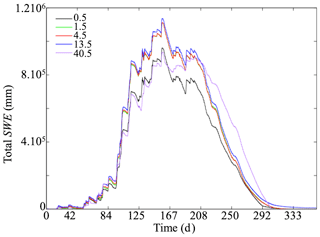
Figure 3 Temporal variations of the total snow water equivalent (SWE) obtained with meteorological forcing at spatial resolutions of 0.5, 1.5, 4.5, 13.5, and 40.5 km.

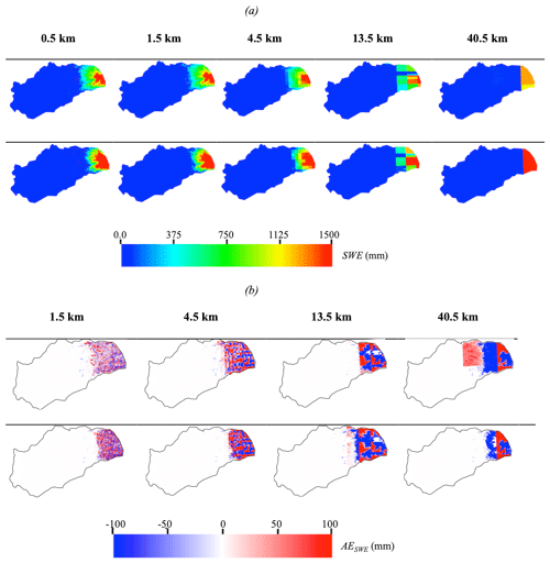
Figure 4a shows the spatial distributions of SWE obtained with the five spatial resolutions at two selected days, which correspond to the beginning (January) and peak (March) of snow accumulation. The spatial distribution of SWE is more precise for results obtained with the higher-resolution meteorological forcing. SWE distributions obtained with meteorological forcing of resolutions at or above 13.5 km are not well estimated. Figure 4b shows the spatial distribution of the absolute error of SWE (AE_SWE). Over- and underestimations of SWE with similar magnitudes are observed for all the four resolutions. Errors in SWE distribution increase (with AE greater than 100 mm) as the resolution of the forcing data decreases. We notice that over- and underestimations of SWE depend both on the topography and the resolution of forcing as snow processes depend not only on the meteorological conditions but also on the slope and aspect of a given hillslope. Depending on the elevation and the orientation of the cell (north and south facing), the energy fluxes are different resulting in very different snow dynamics. This strengthens the conclusions drawn previously stating that the meteorological data should be at a resolution close to the one associated with the input data (e.g., topography) as well as the physics-based model to ensure a good precision and accuracy in the representativity of the snow dynamics. We further note that differences in SWE will lead to different snowmelt, ET, and infiltration rates, which will have implications for other hydrologic variables such as streamflow and groundwater levels.

Figure 4 Spatial distributions of (a) SWE obtained with the five spatial resolutions of meteorological forcing and (b) the absolute error of SWE (AE_SWE) with respect to the highest spatial resolution of meteorological forcing (0.5 km). Results are shown at WY days 125 (January) and 166 (March).

4.2 Evapotranspiration (ET)

Figure 5 shows the temporal variation of the percent error in the domain-average ET (PE_ET) flux as calculated with Eq. (6). We note that the percent error has large values due to the low values of ET; thus small changes in ET result in large percent errors. While in general, the coarsest spatial resolution of forcing (i.e., 40.5 km) shows the highest errors for some time steps, the percent errors obtained with the second-coarsest meteorological forcing (13.5 km) are actually the largest. A possible explanation is the aggregated nature of the domain-average ET. Depending on the time step, the coarser forcing resolutions can lead to either an over- or underestimation of ET. Results do not show a systematic trend with regards to the over- or underestimation of ET. It is therefore difficult to establish a clear relationship between the spatial resolution of forcing and the directionality of ET error at a watershed scale. Note, however, that these errors do not increase over time. This can be related to the fast-changing nature of ET that is strongly linked to short-lived weather patterns and the diurnal cycle.

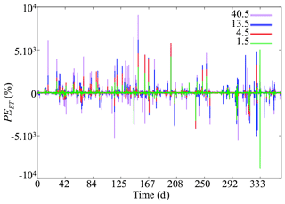
Figure 5 Temporal variation of the percent error of evapotranspiration PE_ET obtained with meteorological forcing at spatial resolutions of 1.5, 4.5, 13.5, and 40.5 km relative to the highest spatial resolution of meteorological forcing (0.5 km).

Figure 6a shows the spatial distributions of ET for the five resolutions at two selected time steps characterizing periods with and without precipitation events. Day 0 corresponds to a dry day in October, and day 167 corresponds to a wet day in March. The spatial patterns of ET at these two time steps are different. Furthermore, spatial patterns between the different scales of forcing also reveal distinct ET patterns. As expected, the most accurate ET distribution is obtained with the highest resolution of the meteorological data; the coarser a resolution of meteorological data is, the less accurate the spatial distribution of ET is. Because the highest resolution of forcing is close to the resolution of the integrated hydrologic model (and thus the resolution of input data such as topography, geology, and land use and land cover), it allows us to better understand the relationships between ET and these different characteristics of the watershed. Such analyses are difficult to undertake for coarser resolutions.

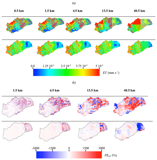
Figure 6 Spatial distributions of (a) the ET obtained with the five spatial resolutions of meteorological forcing and (b) the percent error of ET (PE_ET) with respect to the highest spatial resolution of meteorological forcing (0.5 km). Results are shown at the first day of the simulation (WY day 0, in October) and during the time at which peak differences are observed (WY day 167, in March).

Seasonality and location affect the degree to which forcing scales impact ET. Note that for the spatial distributions of ET associated with the second time step considered (day 167), the results obtained with the five resolutions are very similar in the Central Valley. At this time spatial patterns of ET only differ in the Sierra Nevada Mountains and the intrusion. The geology, as well as the land cover and the topography, is more or less uniform in this valley, whereas these parameters, notably topography, vary significantly in the Sierra Nevada Mountains. For the first time step, the differences observed in the Central Valley are due to the fact that for very precise resolutions of the forcing, the evolution of the storm is accurate (see Appendix A2) and so is the ET. Thus, for relatively homogeneous areas such as the Central Valley, high-resolution forcing data are required only if the storm shows a strong spatial variation within the areas, whereas for highly heterogeneous parameters associated with geology, topography, and land cover, high-resolution forcing data are always required if one is interested in analyzing accurately the spatial distribution of ET.

Figure 6b shows the spatial distributions of percent error of ET (PE_ET) relative to the results of the 0.5 km meteorological forcing. Whatever the resolution considered, we note both an over- and underestimation of ET on the same scale of error (±3000 %) but with more localized and less wide-scale differences at the finest scale of meteorological forcing. We also observe that error is higher in the Sierra Nevada Mountains, characterized by complex topography and geology than in the Central Valley for all resolutions. This reinforces the conclusions drawn previously, namely that for complex environments a precision in the meteorological data is strongly required.

4.3 Infiltration

Figure 7 shows the spatial distributions of infiltration obtained with the five spatial resolutions (Fig. 7a) and their corresponding percent errors (Fig. 7b) at two selected times corresponding to winter (WY day 83, December; presence of precipitation event) and summer (WY day 291, June; absence of precipitation event). The first time step corresponds to the snow accumulation period, while the second one characterizes the snowmelt period. The spatial resolution of forcing data strongly impacts the spatial distribution of infiltration. Indeed, for coarse resolutions (i.e., 40.5 km), it is almost impossible to determine the position of the storm and its impact on infiltration; the results obtained at this scale are strongly dependent on the resolution of the forcing. However, for a more precise resolution (i.e., 0.5 km), we can exactly see the location of the storm; this resolution allows for distinguishing areas characterized by a very weak infiltration as the upper part of the catchment corresponding to the Sierra Nevada Mountains. Indeed, in this area, due to the accumulation of snow (precipitation is in the form of snow unlike in the Central Valley), the resulting infiltration is zero. The spatial extension of the area subject to the snow accumulation is only accurate for high-resolution meteorological-forcing results.

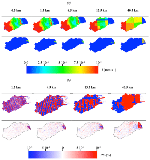
Figure 7 Spatial distributions of (a) infiltration I obtained with the five spatial resolutions of meteorological and (b) the percent error of infiltration (PE_I) with respect to the highest spatial resolution of meteorological forcing (0.5 km). Results are shown in winter (WY day 83) and summer (WY day 291).

To better understand how the quality and precision of the spatial distribution of infiltration deteriorates by decreasing the resolution of the input data, Fig. 7b shows the spatial distribution of the PE_I of the four resolutions at the same two time steps. For the first time step, the errors are null in the Sierra Nevada Mountains, which is not the case for the second time step. Whatever the resolution considered, and as previously discussed, we note that depending on the point considered there may be over- and underestimation of the infiltration with percent error close to 10⁻³. Note that these differences are observed over the entire watershed except in the Sierra Nevada Mountains for the first time step, while for the second time step, these errors are only observed along the river and its tributaries as well as in the Sierra Nevada Mountains. This second time step corresponds to the summer, a snowmelt period and without rain. As such, differences of infiltration in the Sierra Nevada Mountains are due to the snowmelt. As for the differences observed close to the areas subject to the overland flow, these are due to the exchanges between the surface flow and the subsurface. Because the amount of snow accumulated as well as the spatial extent of the area subject to snow dynamics is different for the five resolutions considered, the resulting snowmelt is different. Thus, the runoff controlled by this snowmelt will also be different and so is the infiltration of the quantities of water coming from the overland flow. This indicates that the effects of the spatial resolution of forcing data can be delayed in time.

4.4 Surface and subsurface flow

4.4.1 Surface water storage and river stage

Figure 8 illustrates the percent error of surface water storage PE_SW. In general, the percent error of the surface water storage is small (<5 %) regardless of the time of the year, and these differences are almost zero for the results obtained with 1.5 and 4.5 km forcing resolutions for the entire water year. As shown in Fig. 9 illustrating the spatial distributions of the absolute error of surface pressure head (AE${}_{{\mathrm{\Psi }}_{\mathrm{s}}}$), the percent error of the total surface water storage at the watershed scale is small because some regions in the domain overestimate the pressure head, while others underestimate the pressure head. In contrast, while the error is negligible at the beginning of the simulation for results obtained with forcing at 13.5 and 40.5 km, the PE_SW increases over time, eventually reaching a near-maximum value at the end of the water year. This suggests that PE_SW may be cumulative and that longer simulations with overly coarse scales of forcing will compound through time. It is interesting to also note that while the results obtained with the 13.5 km resolution forcing overestimate the surface water storage at any time, those obtained with the 40.5 km resolution forcing show overestimates of PE_SW at the beginning of the simulation and underestimates of PE_SW at the end of the simulation. Moreover, the errors obtained with the 13.5 and 40.5 km resolution are of the same order but opposite signs. This suggests that although the total water budget is nearly equivalent for each scale of forcing considered here (see Appendix A1), an inaccurate spatial distribution of forcing can lead to an inaccurate redistribution (and possibly a delay) of water and energy and hence different signals of surface water storage.

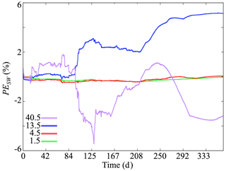
Figure 8 Temporal variations of the percent error of surface water storage (PE_SW) obtained with meteorological forcing at spatial resolutions of 1.5, 4.5, 13.5, and 40.5 km with respect to the highest spatial resolution of meteorological forcing (0.5 km).

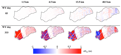
Figure 9 Absolute error of surface pressure head (AE${}_{{\mathrm{\Psi }}_{\mathrm{s}}}$) with respect to the highest spatial resolution of meteorological forcing (0.5 km). Results are shown in winter (WY day 83, in December) and summer (WY day 333, in August).

Figure 9 shows the spatial distributions of the absolute error of pressure head for the first layer (AE${}_{{\mathrm{\Psi }}_{\mathrm{s}}}$) at two selected time steps corresponding to winter (WY day 83, in December) and summer (WY day 333, in August). Similar to PE_SW, this error increases with time. In December, the error is nearly zero for forcing spatial resolutions of 1.5 and 4.5 km, whereas it is nonzero (with values close to 1 m) in August. Although the spatial resolutions of 13.5 and 40.5 km have nonzero errors at the first time step, the error increases considerably as the simulation proceeds. We note that the areas sensitive to the spatial resolution of the meteorological-forcing data are approximately the same for all four resolutions. Indeed, the absolute error is null at the intrusion, contrary to the Central Valley and in the Sierra Nevada Mountains. Interestingly, these two zones have different areas of influence: in the Central Valley, the errors are nonzero everywhere except close to the river, which is contrary to the trend observed in the Sierras. This is related to the geological nature of these environments. Due to the very low permeability and low surface roughness of Sierra Nevada Mountains, any water from precipitation will quickly contribute to surface runoff, which is highly sensitive to the spatial resolution of forcing, contrary to the Central Valley, which is characterized by high permeability and a low Manning coefficient and therefore low overland flow.

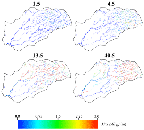
Within the water year, the maximum absolute error of surface water levels max(AE${}_{{\mathrm{\Psi }}_{\mathrm{s}}}$) is an important metric for understanding where, and to what degree, forcing resolution impacts the prediction of river dynamics. Figure 10 shows the spatial distribution of max(AE${}_{{\mathrm{\Psi }}_{\mathrm{s}}}$), which is obtained by an analysis of the maximum difference in surface water levels between the results obtained with the highest spatial resolution of forcing (0.5 km) and the four other resolutions for all time steps. Maximum differences in surface water levels are shown in absolute values (in units of meters) and are at any point in time in the simulated water year. Differences in surface water levels at a given time are as high as 3 m. High values of differences are mainly located in the headwater region of the watershed, although some lower regions of the model such as one tributary of the main stem of the Cosumnes near the river outlet also show max(AE${}_{{\mathrm{\Psi }}_{\mathrm{s}}}$) as high as 3 m. These results suggest that although the impact of forcing spatial resolutions on the global (i.e., watershed-scale) surface water storage is small to insignificant (see Fig. 8), at a given point in space and time, differences may be considerable. This can be especially problematic for calibration and validation purposes where input parameters of the model are adjusted to reproduce the observed surface water levels with the model. In this case, differences between measured and simulated hydrologic variables are assumed to be due to parametric uncertainties, when in reality the source of the error is the scale of the meteorological forcing. Adjusting the model parameters may potentially cause the model to inaccurately simulate the physics of the system.

Figure 10 Spatial distributions of the maximum of the absolute error of river height max(AE${}_{{\mathrm{\Psi }}_{\mathrm{s}}}$) with respect to the highest spatial resolution of meteorological forcing (0.5 km).

4.4.2 Groundwater storage and water table depth

Figure 11 depicts the percent error of groundwater storage PE_GW. For the cases considered here, the different spatial resolutions of forcing have very little impact on the total groundwater storage of the watershed.

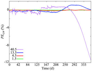
Figure 11 Temporal variations of the percent error of groundwater storage (PE_GW) obtained with meteorological forcing at spatial resolutions of 1.5, 4.5, 13.5, and 40.5 km with respect to the highest spatial resolution of meteorological forcing (0.5 km).

With the exception of the coarsest scale of forcing resolution towards the end of the simulation, the error in groundwater storage for the different spatial resolutions of forcing yield very similar results. Groundwater storage obtained with a forcing resolution of 13.5 km overestimates the storage; however, this overestimation remains very low, on the order of 1 % at most times. In contrast, the groundwater storage results obtained with the 40.5 km forcing resolution are close to the storage obtained with the finest scale of forcing resolution at the beginning of the simulation, yet these errors reach 10 % at the end of the simulation.

Figure 12a shows the maps of water table depth (WTD) absolute error (AE_WTD) for the four scales of forcing resolution relative to the results obtained with the 0.5 km forcing. Water year day 333 (August) corresponding to baseflow conditions is used here because differences in water table depth at the beginning of the simulation are too small for interpretation. Results show both an over- and underestimation of the water table depth as a function of the forcing resolution (Fig. 12a). Thus, while the global groundwater storage error is low as indicated in Fig. 11, an examination of the spatial trends shows that this is predominantly due to the counterbalancing of positive and negative error in space. For all the spatial resolutions considered, the Sierra Nevada Mountains are the most sensitive areas to the spatial resolution of meteorological data, while the intrusion remains insensitive with almost zero errors. This is due to the characteristics of the Sierra Nevada Mountains which include strong variations of topography, snow dynamics, and low-permeability rocks. The intrusive zone is composed of extremely low-permeability materials, so it has no groundwater dynamics; as such the errors are zero. The spatial resolutions of 1.5 and 4.5 km have generally little impact on the water table depth in the Central Valley alluvial aquifers. Larger errors in water table depths are mostly observed for the results obtained with the 13.5 and 40.5 km forcing. These errors are not uniform and are most significant along the Cosumnes River, its tributaries, and outside urban areas. The connection between the upper and lower point of the watershed, as well as the integrated nature of the system, is apparent in the maps of AE_WTD. As already discussed, because the spatial resolution of forcing impacts snowpack dynamics, evapotranspiration and infiltration rates and patterns, and streamflow distributions, it, therefore, impacts groundwater dynamics and the exchange of groundwater and surface water. We highlight here that these differences accumulate over time as indicated by the errors that increase as the simulation progresses.

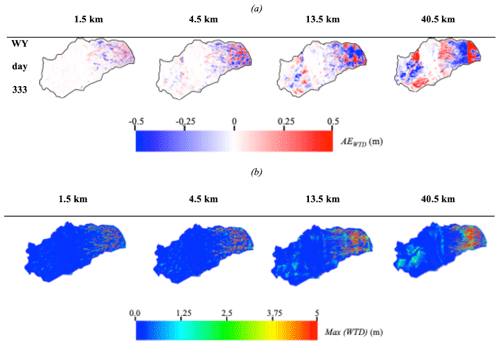
Figure 12 Spatial distributions of (a) the absolute error of water table depth (WTD) (AE_WTD) with respect to the highest spatial resolution of meteorological forcing (0.5 km) at WY day 333 and (b) max(AE_WTD) with respect to the highest spatial resolution of meteorological forcing (0.5 km).

Figure 12b depicts the maximum differences (for all time steps) of the water table depth in absolute values between the results obtained with the highest spatial resolution and the other four spatial resolutions. As previously stated, due to the almost zero permeability of the intrusion, the latter is insensitive to the spatial resolution of the meteorological data. The water table depth differences are as high as 5 m in several places, particularly in the Sierra Nevada Mountains, following mostly trends in topography. In the Central Valley, noticeable differences are mainly observed in the areas near the rivers and close to the pumping wells.

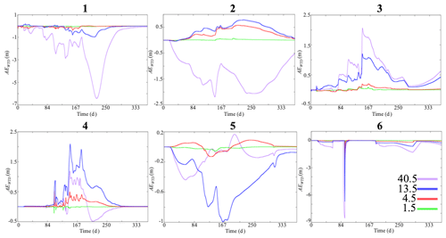
Figure 13 shows the temporal variations of the difference in the water table depth between the highest resolution and the four other resolutions at six selected points. We selected points located in the Central Valley, as this zone hosts an alluvium aquifer (see their location in Fig. 1). For all these points, we note that the differences are almost zero for the spatial resolution of 1.5 km, indicating that this spatial resolution is sufficient to represent the groundwater dynamics of this region. The spatial resolution of 4.5 km also shows relatively low differences; the latter is indeed zero at three points, and only points 2, 4, and 5 have nonzero differences, but these remain less than 50 cm. The strongest differences are observed for results obtained with forcing spatial resolutions of 13.5 and 40.5 km; note that the coarsest resolution does not necessarily give the highest differences. In fact, at points 4 and 5, the highest differences are obtained with the resolution of 13.5 km, indicative of the complex over- and underestimation patterns of bias observed at these coarser resolutions of forcing. In general, the use of these large-scale spatial resolutions of forcing can lead to an over- or underestimation of the pressure head between 50 cm and 10 m. Thus, while our results indicate that the spatial resolution of meteorological forcing has little impact on the total groundwater storage, at discrete points within the watershed the spatial resolution of forcing is very important, especially for resolutions greater than 4.5 km. Again, this is particularly an issue for model calibration purposes given that hydrologic numerical models are typically validated and calibrated by comparing the groundwater measurements with the model outputs. In this case, our results indicate that careful attention must be given to the spatial resolutions of forcing, as some errors are only due to the latter not to any model parameterization.

Figure 13 Absolute error of the water table depth (AE_WTD) with respect to the highest spatial resolution of meteorological forcing (0.5 km) at six selected points.

5 Conclusions

Numerical methods that solve integrated hydrologic models are becoming increasingly precise and spatially resolved. They thus require high-resolution and accurate input data such as meteorological forcing. However, while integrated hydrologic models increase in precision, the meteorological data used are most often of coarse resolution, whereas these data are strongly heterogeneous in space. It is, therefore, important to better understand not only how the uncertainties associated with the spatial distribution of meteorological data affect hydrologic model outputs but also the meteorological-forcing spatial resolution required to minimize these uncertainties. Moreover, thanks to the advancement of atmospheric models, it is now possible to obtain meteorological data closer to that of the resolution of hydrologic models.

In this study, we utilized the integrated hydrological model ParFlow-CLM to simulate the hydrodynamics of a representative Californian watershed spanning the Sierra Nevada Mountains and the Central Valley interface. The Cosumnes offers a unique opportunity to study semi-natural flow conditions, given that it is a rare undammed river, one of the last in the state. Five different spatial resolutions of meteorological data were obtained via the dynamical downscaling approach of the Weather Research Forecasting (WRF) model. Both models were simulated in a high-performance computing environment to accommodate the high spatiotemporal resolution of the study. The Cosumnes watershed is characterized by strong variations of topography, geology, and land use and land cover leading to highly heterogeneous and complex atmospheric and hydrologic dynamics and is, therefore, an excellent candidate to better understand how the different spatial resolutions of forcing affect the results of an integrated hydrologic model of a watershed, which include snow water equivalent, evapotranspiration, infiltration, and surface and groundwater levels.

Our results show that the impact of the spatial resolution of meteorological data depends on the hydrologic component of interest, as well as the temporal and spatial scale.

• Snow accumulation and snowmelt are considerably impacted by forcing resolution, even at the watershed scale. The results obtained with the different spatial distributions suggest that meteorological data with a resolution close to the one of the hydrologic model is needed to accurately reproduce the snow water equivalent (SWE) distribution as well as the total volume of SWE. Our results show that the errors of SWE depend on both the spatial resolution of forcing and topography and can be greater than 100 mm for a single point in time.

• At the watershed scale, global estimates of total evapotranspiration fluxes are more or less insensitive to the spatial resolution of forcing. However, to obtain an accurate spatial distribution of evapotranspiration which shows impacts of land use, geology, and topography, higher resolutions of forcing are needed.

• The results obtained with infiltration are quite similar to those of evapotranspiration. Note that for these two processes, the percent errors induce by a coarser resolution are most often significant after a precipitation event and that these errors quickly subside once the precipitation ends.

• Forcing spatial resolution does not impact total surface water storage at the watershed scale. Even for the coarsest resolution of forcing (40.5 km), the error, increasing with time, is approximately 5 %. However, we emphasize that for the surface water levels at one point and at a given time, the differences between the highest spatial resolution of the forcing data and the four other resolutions can exceed 3 m. Regions within the Sierra Nevada Mountains are the most sensitive to the spatial resolution of forcing data.

• Similar to surface water storage, the five different spatial resolutions of forcing considered in this study led to similar groundwater storages. Therefore, the spatial resolution of forcing has very small impacts on the hydrology simulated at a watershed scale or hydrologic unit; hence non-grid-based hydrologic models are likely to be less sensitive to the spatial resolution of forcing than numerical models. However, at a local scale, the variations of pressure head in the subsurface obtained with the different resolutions can differ considerably, with error as high as 9 m, especially in the Central Valley alluvium aquifers. Groundwater level variations are the result of the aggregated impacts of land surface processes. As such, the spatial resolutions of forcing affecting land surface processes also impact groundwater levels. Our results show that these impacts on groundwater are delayed in time due to the timing of the transfer of water from the land surface to the subsurface.

Although the total water balance of the five spatial resolutions of the meteorological forcing is the same, the different spatial resolutions lead to different hydrological processes that change both in time and space. For a good representation of the land surface processes (infiltration, evapotranspiration, and snow dynamics), a spatial resolution of the meteorological data which is close to that of the hydrologic model is required due to the instantaneity and complexities of these phenomena. For the surface and subsurface processes, we demonstrated that for this watershed and those with similar characteristics, a spatial resolution of 4.5 km is sufficient to reproduce the general physical trends of the hydrology. As a result, satellite-based products such as NLDAS (with a resolution of around 14 km) may induce errors that may limit the use of their products if spatially accurate studies are needed. Because coarse spatial resolutions of forcing may lead to very different groundwater and streamflow variations, particular attention must be paid to the spatial resolution of meteorological data, especially in the calibration and/or validation processes of numerical models. Indeed, the differences between the measured and simulated hydrologic variables are not only due to the hydrodynamic parameters of the model but may also be related to the parameterization of the meteorological data.

While in this study our focus is on the spatial distribution of meteorological data, future studies will assess the propagation of uncertainties related to the temporal resolution of meteorological forcing. Climate models are also used to predict the future weather conditions; it would also be important to determine the ideal spatial resolution of forcing in the context of a warming climate. Because, Hydrologic Response Unit-based (HRU) hydrologic models are also commonly used, future work could further assess the sensitivity of these models to the spatial distribution of meteorological data.

Appendix A

A1 Mass balance validation

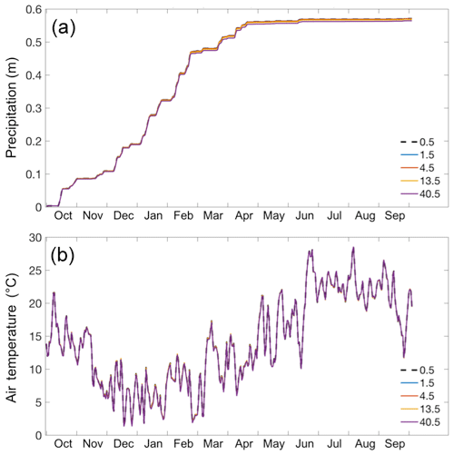
The physics represented for the four WRF domains are identical, except for cumulus parameterization which is used for domains d01 (resolution of 13.5 km) and d02 (resolution of 13.5 km) and not for domains d03 (resolution of 1.5 km) and d04 (resolution of 0.5 km). This is due to the fact that WRF can resolve convection explicitly at resolutions higher than around 4 km (Gilliland and Rowe, 2007). To assess the sensitivity of the WRF-simulated forcings to this inevitable inconsistency between the domains, we compare watershed-wide daily precipitation and air temperature in Fig. A1. Our results show that there are minimal differences (RMSE of less than 0.002 m and 0.01 ^∘C for precipitation and temperature, respectively) between the four WRF domains, when averaged over the watershed. This shows that the only differences between the forcings from WRF domains are due to different resolutions, and the effects of described differences in physics representations are limited.

Figure A1 Daily variations of WRF-simulated precipitation (a) and air temperature (b), averaged over the entire watershed for spatial resolutions of 0.5, 1.5, 4.5, 13.5, and 40.5 km.

A2 Spatial distributions of precipitation and temperature over domain d04

Figure A2 Spatial distributions of precipitation associated with the five spatial resolutions of meteorological forcing at three selected times corresponding to periods where the storm has high (day 1) and low (day 83) intensity and a time of very located and low intensity (day 125).

Figure A3 Spatial distributions of temperature associated with the five spatial resolutions of meteorological forcing at three selected times corresponding to periods where the storm has high (day 1) and low (day 83) intensity and a time of very located and low intensity (day 125).

A3 Comparisons with ground measurements

We compared simulated precipitation and temperature with ground measurements. We selected four stations, which continuously measure precipitation and temperature. The figure below shows the location of these stations as well as the comparisons. We only show comparisons with the results obtained with the highest resolution (i.e., d04) for graphical purposes.

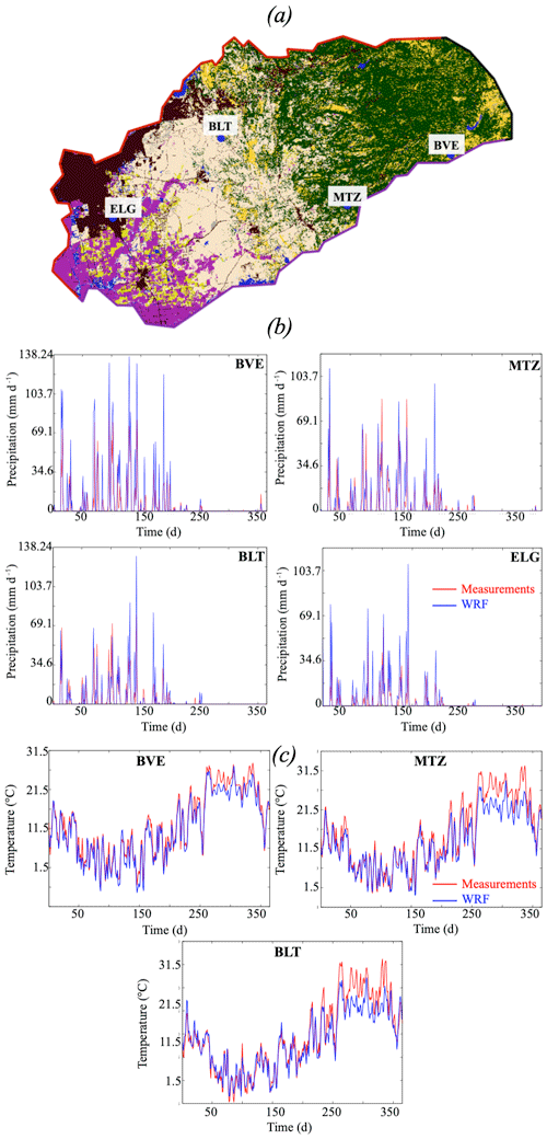
Figure A4 (a) Location of the four selected stations. These stations allow for comparing the simulated precipitation and temperature with measurements in the Sierra Nevada Mountains (BVE and MTZ), the volcanic intrusion (BLT), and the Central Valley (ELG). (b) Comparisons between simulated and measured precipitation at the four selected stations. The reasonable match between measurements and simulations at different locations allows for gaining confidence in the WRF simulations to reproduce the atmospheric dynamics at different elevations. (c) Comparisons between the simulated and measured temperature at three selected stations. The station ELG does not have measurements of temperature. Like the precipitations results, our comparisons indicate a reasonable match between measurements and simulations.