Assessing the impact of seasonal-rainfall anomalies on catchment-scale water balance components

Although water balance components at the catchment scale are strongly related to annual rainfall, the availability of water resources in Mediterranean catchments also depends on rainfall seasonality. Observed seasonal anomalies in historical records are fairly episodic, but an increase in their frequency might exacerbate water deficit or water excess if the rainy season shortens or extends its duration, e.g., due to climate change. This study evaluates the sensitivity of water yield, evapotranspiration, and groundwater recharge to changes in rainfall seasonality by using the Soil Water Assessment Tool (SWAT) model applied to the upper Alento River catchment (UARC) in southern Italy, where a long time series of daily rainfall is available from 1920 to 2018. We compare two distinct approaches: (i) a “static” approach, where three seasonal features (namely rainy, dry, and transition fixed-duration 4-month seasons) are identified through the standardized precipitation index (SPI) and (ii) a “dynamic” approach based on a stochastic framework, where the duration of two seasons (rainy and dry seasons) varies from year to year according to a probability distribution. Seasonal anomalies occur when the transition season is replaced by the rainy or dry season in the first approach and when season duration occurs in the tails of its normal distribution in the second approach. Results are presented within a probabilistic framework. We also show that the Budyko curve is sensitive to the rainfall seasonality regime in UARC by questioning the implicit assumption of a temporal steady state between annual average dryness and the evaporative index. Although the duration of the rainy season does not exert a major control on water balance, we were able to identify season-dependent regression equations linking water yield to the dryness index in the rainy season.

1 Introduction

The rainfall regime of the Mediterranean climate is characterized by the alternation of wet and dry periods within the year, with evident out-of-phase seasonal behavior of precipitation and temperature patterns. Most annual rainfall is concentrated in the late fall, winter, and early spring, while late spring, summer, and early fall are usually hot and quite dry. Rainfall seasonality plays a fundamental role in planning and managing water resources in countries subject to a Mediterranean climate. Summer is characterized by water stress due to scarce rainfall supply, combined with high evapotranspiration loss and the seasonal peak in water consumption (comprising agricultural, industrial, and recreational uses, hydroelectric power generation, and domestic uses, which are often boosted by tourism pressure). Therefore, it is necessary to store water during the rainy period to cope with the uncertain duration of adverse water deficit conditions during the dry period. Water supply infrastructures necessitate high investment costs that strongly depend on the expected balance between the amount of water supplied in the rainy period and the amount of water lost and consumed during the dry season. The amount of rainfall in each season can be suitably decomposed and simulated on the basis of the following three main components: (i) duration of the seasons, (ii) occurrence probability of a daily rainfall event in each season, and (iii) mean depth of daily rainfall events in each season (Van Loon et al., 2014). A combination of the last two factors determines the rainfall magnitude in each season (Feng et al., 2013).

A very small or very large amount of water (exceeding a certain threshold value for a specified return period and duration) supplied in each season can be interpreted as a seasonal precipitation anomaly and is usually observed episodically in a historical multidecadal time series of annual rainfall values. Seasonal precipitation anomalies result mainly from a combination of the duration of the wet season and its rainfall magnitude. These two factors should be taken into due account when planning water supply infrastructures (Apurv et al., 2017). The most recent reports released by the Intergovernmental Panel on Climate Change (IPCC, 2013) warn of the projected increase in seasonal anomalies induced by global warming in the Mediterranean region, with a considerable decrease in annual precipitation and warming-enhanced evapotranspiration associated with rather severe and prolonged droughts, as recently observed in southern Europe in 2003, 2015, and 2017 (Mariotti et al., 2008; Laaha et al., 2017; Hanel et al., 2018).

Studies underway in the upper Alento River catchment (UARC) in southern Italy offer a good chance to understand the effects of seasonal-rainfall uncertainty on water supply generation given the presence of a multipurpose earthen dam (known as Piano della Rocca) constructed to regulate water for irrigation, hydropower generation, flood control, and drinking purposes. The main research question, also raised or prioritized in some way by local stakeholders in their decision-making processes, can be expressed as follows: what is the impact of seasonal-rainfall anomalies on annual (or seasonal) average water supply in UARC? This question is particularly relevant to hilly catchments similar to UARC within the Mediterranean region such that UARC could become a pilot area for dealing with some specific problems and carrying out paired-catchment analyses.

This study therefore aimed to quantify the effects exerted by seasonal-rainfall anomalies on water balance components. With a view to coordinating interaction with stakeholders, end users, and professionals, we performed this task by implementing the well-known and well-validated Soil Water Assessment Tool (SWAT) model (Arnold et al., 1998). Particular attention is devoted to computing water yield supplying the artificial reservoir bounded by the Piano della Rocca earthen dam in ARC (Alento River catchment; Romano et al., 2018). One of the strengths of our approach lies in the availability of long-term rainfall time series (about a century of daily data) and detailed soil and land cover maps, enabling reliable catchment-scale model simulations. Reliable scenario-based projections are built to investigate whether the longer-than-average duration of the wet season implies a higher-than-average mean annual rainfall and consequently higher-than-average water yield. To investigate this issue, our research strategy couples the seasonal duration with daily rainfall occurrences and depths by using a Monte Carlo approach to obtain SWAT-simulated water balance components within a general probabilistic framework.

Many authors have attempted to quantify rainfall seasonality using different approaches (Markham 1970; Nieuwolt, 1974; Oliver, 1980; Walsh and Lawler, 1981; Zhang and Qian, 2003; Martin-Vide, 2004; Potter et al., 2005; Feng et al., 2013; de Lavenne and Andréassian, 2018). The precipitation concentration index (PCI) proposed by Oliver (1980) is the most popular approach for quantifying the year-round precipitation distribution in a given study area (Raziei, 2018). Sumner et al. (2001) analyzed the spatial and temporal variation of precipitation seasonality over eastern and southern Spain by using the seasonality index (SI). The SI was also utilized to examine the spatial and temporal variability of precipitation seasonality in Greece (Livada and Asimakopoulos, 2005), the USA (Pryor and Schoof, 2008), and northern Bangladesh (Bari et al., 2017). Under the typical Mediterranean climate of Sardinia (Italy), Corona et al. (2018) used the SI to evaluate the role of precipitation seasonality on runoff generation. Nonetheless, while the PCI and SI are useful indexes to classify rainfall seasonality and the degree of concentration of rainfall within the year, their implementation in a Monte Carlo framework is not straightforward. Therefore, we opted to characterize rainfall seasonality and its anomalies by using the two approaches described as follows. A first approach, which is hereafter referred to as the static approach, is based on the analysis of the standardized precipitation index (SPI) to define the duration of a wet season (4 months), a dry season (4 months), and a transition season (2 months from the dry-to-wet phase plus 2 months from the wet-to-dry phase) in UARC. In this approach, the drought anomaly is rigidly built with the artifact of extending the duration of the dry season to 8 months by removing the transition season. The same criterion applies to a prolonged duration of the rainy season. The second approach, instead, exploits the seasonality characterization proposed by Feng et al. (2013) and can be viewed as a dynamic approach, since the duration of the rainy season is time variant (inter-annual variability) and can be stochastically generated with random duration values drawn from their statistical distribution. This second approach investigates what happens to the water budget if the duration of the rainy season becomes shorter than normal (i.e., rainfall scarcity) or longer than normal (i.e., rainfall excess). As far as we are aware, there is still a lack of knowledge about the effects of possible changes in rainfall seasonality on the water balance of a catchment subject to a Mediterranean climate, and the analyses presented in this paper aim primarily to contribute to fill this gap.

2 Study area and experimental analyses

The upper Alento River catchment (UARC) is situated in the southern Apennines (Province of Salerno, Campania, southern Italy) and has a total drainage area of about 102 km² (Fig. 1). The elevation spans between 88 and 1298 m a.s.l., and the average slope is about 14.4^∘. The Piano della Rocca dam is an earthen embankment with an impervious core that has been operating since 1995. The area consists mostly of mountain and hill country with relatively poorly permeable arenaceous–clayey deposits and secondarily of arenaceous–marly–clayey and calcareous–clayey deposits (Romano et al., 2018).

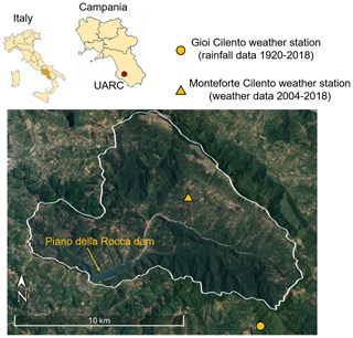
Figure 1 Geographical position of the upper Alento River catchment (UARC) in Campania (southern Italy) with the locations of the weather stations of Gioi Cilento and Monteforte Cilento. This figure was adapted from © Google Maps.

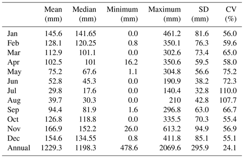
A weather station (699 m a.s.l.) managed by the Italian Hydrological Service is located near the village of Gioi Cilento and provides a dataset of daily rainfall values covering the period of 1920–2018 (about 90 years), with an interruption of 9 years (1942–1950) straddling World War II (Nasta et al., 2017). The dataset of annual rainfall sums derived from the daily rainfall time series has a mean of 1229.3 mm, while other metrics (median, standard deviation, and coefficient of variation) are reported in the last row of Table 1. The same statistics are also summarized for rainfall depths in each month of the year. The variability exhibited by the monthly time series of rainfall depths is also depicted in Fig. 2, denoting a typical Mediterranean seasonal cycle. A large amount of precipitation occurs in the months from October to March, a period commonly identified as a wet period of the hydrological year, and accounts for about 68 % of the annual mean rainfall (i.e., 834.9 mm over 1229.3 mm; see Table 1 and Fig. 2). November is the wettest month with an average monthly rainfall of 166.9 mm (about 14 % of mean annual rainfall). In contrast, lower mean monthly rainfall depths are concentrated from April to September, which commonly identify a dry period of the hydrological year, with a cumulative rainfall over this period of 394.5 mm with respect to the annual mean of 1229.3 mm, hence representing about 32 % of mean annual rainfall. July is the driest month with a monthly mean rainfall of 29.8 mm (i.e., 2 % of mean annual rainfall).

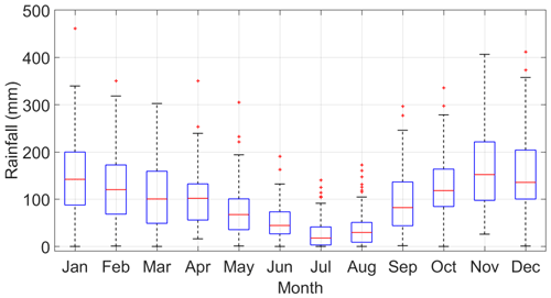
Figure 2 Box plots of monthly rainfall depths recorded at the Gioi Cilento weather station (1920–2018).

Table 1 Descriptive statistics of the monthly and annual rainfall distributions recorded at the Gioi Cilento weather station during the period of 1920–2018. SD: standard deviation; CV: coefficient of variation.

Within the monitoring activities of the MOSAICUS (MOnitoring and modeling Soil–vegetation–atmosphere processes in the Alento river basin for Implementing adaptation strategies to Climate and land USe changes) project (Nasta et al., 2013; Romano et al., 2018), an automated weather station (400 m a.s.l.) was installed in 2004 close to the village of Monteforte Cilento and equipped with sensors for monitoring rainfall, wind speed and direction, air temperature and relative humidity, and solar radiation to record such meteorological variables at 60 min intervals (Nasta et al., 2019). The statistical distributions of weather data recorded at the weather station of Monteforte Cilento (2004–2018) will be used to calculate potential evapotranspiration as described in Sect. 3.

In this study, we used the most recent available land use map drawn up in 2015 by using second-level CORINE (Coordination of Information on the Environment) Land Cover classes (CORINE 2006 Land Cover dataset; http://www.eea.europa.eu, last access: 6 March 2015): forest, arable land (annual crops), permanent crops (orchards, vineyards, olive groves, and fruit trees), pasture, urban fabric, and water bodies. Forest (evergreen and deciduous trees and multi-stem evergreen sclerophyllous Mediterranean shrubs) and agricultural (arable land, permanent crops, and orchards) cover about 70 % and 20 % of the catchment, respectively (Nasta et al., 2017). A 5 m resolution digital terrain model (DTM) was used to generate the hydrographic network and a soil landscape unit map is used to depict soil attributes in UARC (Nasta et al., 2018).

3 Parameterization of the SWAT Model

The Soil Water Assessment Tool (SWAT) is a bucket-type, semi-distributed hydrological model operating on a daily timescale and at a catchment spatial scale (Arnold et al., 1998). The main components of the water balance equation are the daily change in water storage (ΔWS) as affected by rainfall (R), actual evapotranspiration (ET_a), groundwater recharge (GR), and water yield (WY). Water yield is given by the contribution of surface runoff, groundwater circulation, and lateral flow within the soil profile and is partially depleted by transmission losses from tributary channels and water abstractions. All variables are expressed in units of millimeters of water height.

SWAT requires as input rainfall (R) and potential evapotranspiration (ET_p) time series at a daily scale and is based on the concept of hydrological response units (HRUs), which are areas identified by similarities in soil, land cover, and topographic features, where hydrological processes are represented by a lumped schematization. The 5 m DTM of the study area was used to determine the catchment boundaries, the hydrographic network, and 13 distinct HRUs. Catchment-lumped parameters are assigned to each HRU through lookup tables. By using the available soil landscape unit map, the input parameters were assigned according to the model setup as presented in Nasta et al. (2017). Nine parameters were calibrated to achieve the best model fit between simulated and measured monthly water yield data recorded from 1995 and 2004 (Nasta et al., 2017). Such hydrological parameters include the soil evaporation and compensation factor, the plant uptake compensation factor, Manning's value for overland flow, the baseflow recession constant (groundwater flow response to changes in recharge), groundwater delay time, the groundwater “revap” coefficient (controlling water that moves from the shallow aquifer into the unsaturated zone), Manning's coefficient for the main channel, the effective hydraulic condition in the main channel alluvium, and the bank storage recession curve. Model performance proved to be satisfactory at a monthly timescale. We ran numerical simulations at a daily time step (rainfall was randomly generated at a daily time step) and aggregated the output fluxes at a monthly time resolution. Although there is evidence in the body of scientific literature of a potential misfit between measured and simulated water yield values at a daily timescale when calibrating a model with data at a monthly time resolution (Adla et al., 2019), we are confident that our results and conclusions will not be affected by this drawback. Our analysis is based on the monthly aggregation of fluxes and is aimed at analyzing seasonal patterns of monthly aggregates.

This study is based on modeling scenarios implemented in SWAT through a Monte Carlo approach, where each simulation is 3 years long. Results from the first 2-year warmup period are discarded, while water balance components simulated for the third year are stored for subsequent analysis. Initial soil water storage is set as field capacity. The model simulations of the first 2 years are disregarded in order to erase the impact of the initial (unknown) soil moisture values set in the soil domain. We point out that the initial soil water content set at field capacity can be considered a realistic situation in winter under the Mediterranean climate. The rainfall data are generated for the static and dynamic approaches (described below) using a probability setting calibrated on daily rainfall values recorded at the Gioi Cilento weather station (1920–2018). The mean and standard deviation of the meteorological data (wind speed, air temperature and relative humidity, and solar radiation) recorded at the second automated weather station (close to the village of Monteforte Cilento) are calculated each month. Daily potential evapotranspiration data were calculated by using random values of weather data drawn from their normal distribution in each month of the year (Allen et al., 1998). Results were provided as input to SWAT to randomly generate daily potential evapotranspiration by using the Penman–Monteith equation (Allen et al., 1998).

4 Determination of rainfall seasonality

4.1 Static approach based on the SPI drought index

The intra-annual rainfall regime under a Mediterranean climate can be characterized through the distribution of annual rainfall depth among different seasons (Paz and Kutiel, 2003; Kutiel and Trigo, 2014). The seasonal pattern occurring in the study area is here characterized by analyzing the distribution of the standardized precipitation index (SPI) on a long-term monthly rainfall time series. The SPI is a probability index developed to classify rainfall anomalies and often employed as an indicator of potential (meteorological) droughts over many timescales (McKee et al., 1993; Hayes et al., 1999). Computation of the SPI should rely on long-term rainfall datasets (e.g., 30 years, according to climatological standards) and is usually obtained by projecting a gamma distribution fitted on rainfall depths cumulated for 1, 3, 6, 12, 18, or 24 months (referred to as SPI-1, SPI-3, SPI-6, SPI-12, SPI-18, or SPI-24, respectively) into a standardized normal distribution. The short-term SPI (e.g., 3-month timescale) can provide useful information for crop production and soil moisture supply, while the long-term SPI (e.g., 12- or 24-month timescale) can give insights on water availability for groundwater recharge. Negative SPI values indicate drier-than-expected rainfall, whereas positive SPI values refer to wetter-than-expected months. To quantify the degree of departure from median conditions, McKee et al. (1993) proposed a rainfall regime classification. Since the SPI is given in units of standard deviation from the standardized mean, this statistical index enables also the precipitation anomaly to be identified through the magnitude of its value: values ranging from −0.99 to +0.99 are considered near normal, from those +1.00 to +1.49 (or from −1.49 to −1.00) indicate moderately wet (or moderately dry) periods, those from +1.50 to +1.99 (or from −1.99 to −1.50) indicate very wet (or very dry) periods, and those above +2.00 (or below −2.00) indicate extremely wet (or extremely dry) periods. Therefore, the extent of SPI departure from the mean (i.e., from the zero value) gives a probabilistic measure of the severity of a wet (if positive) or dry (if negative) period. By exploiting the properties of the (standard) normal distribution, the probabilities of obtaining SPI values greater than +1, +2, and +3 (or less than −1, −2, and −3) are 15.90 %, 2.28 %, and 0.14 %, respectively.

To emphasize the seasonal cycle of intra-annual rainfall patterns within a probabilistic framework, we used the SPI-1 by fitting the gamma distribution on all monthly rainfall depths, i.e., pooling observations from all months in each year. In such a way, the months characterized by SPI-1 values below, around, or above the zero line can be assumed to belong to the dry, transition, or wet seasons, respectively.

4.2 Dynamic approach based on the duration of the wet season proposed by Feng et al. (2013)

According to Feng et al. (2013), the dimensionless seasonality index (DSI) is based on the concept of relative entropy and quantifies the rainfall concentration occurring in the wet season. The DSI is zero when the average annual rainfall is uniformly distributed throughout the year and maximized at 3.585 when maximum average annual rainfall is concentrated in a single month (Pascale et al., 2016); see the Appendix for details. Feng et al. (2013) proposed to describe the rainfall seasonality through the following three components: annual rainfall depth (magnitude), centroid (timing), and spread (duration) of the wet season (see also Pascale et al., 2015; Sahany et al., 2018). As described in Sect. 5.2 and according to appropriate statistical tests, we found that a normal distribution can reasonably describe the 90 wet-season durations obtained by applying to the observed rainfall time series the procedure proposed by Feng et al. (2013), which is briefly summarized in the Appendix. Thus, each hydrological year will consist of the alternation of only two seasons: the wet season with a duration that is randomly generated by a normal distribution with the mean and standard deviation estimated on the Gioi Cilento time series and a dry season in the subsequent months of the year.

4.3 Setup of Monte Carlo rainfall scenarios in SWAT

Seasonal-rainfall anomalies, although episodic, can affect the water balance components at the catchment scale. As suggested by Domínguez-Castro et al. (2019), the impact of such anomalies can be quantified within a probabilistic framework. For the upper Alento River catchment (UARC), we evaluated the effects of seasonal anomalies by running SWAT simulations with synthetic rainfall time series considering different hypotheses (scenarios) of alternations of seasons, according to the static and the dynamic approaches described above. In each season, we assumed that rainfall evolution in time can be represented by a stochastic Poisson point process of daily rainfall occurrences, with daily rainfall depth following a proper probability distribution (Eagleson, 1972; Rodríguez-Iturbe et al., 1987; Veneziano and Iacobellis, 2002). Synthetic rainfall time series were then generated, keeping constant parameters of the Poisson process and daily rainfall parent distribution in each season.

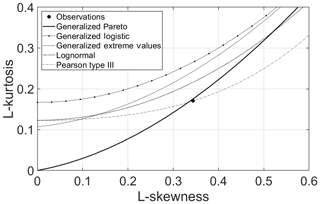
Figure 3 Theoretical L-moment ratio of common distribution models, as compared to the sample L-moment ratios of daily rainfall time series at the Gioi Cilento weather station (large filled circle).

A preliminary analysis was conducted to investigate the best parent distribution for observed rainfall daily depths. With this aim, we used the L-moment ratios diagram proposed by Hosking (1990) (see also Vogel and Fennessey, 1993) as a diagnostic tool. Results are shown in Fig. 3, where the L-skewness and L-kurtosis values computed on the time series left-censored with a threshold of 3 mm (large filled circle) is compared with the theoretical expectation of the same L-moment ratios for several probability distributions commonly adopted in statistical hydrology. An ideal candidate for a parent distribution seems to be the generalized Pareto distribution (GPD), although it is also worth noting that sample estimation of L-skewness and L-kurtosis values (0.3437, 0.1706) is very close to the expected values for exponential distribution (1∕3 and 1∕6). As visual support for this preliminary analysis, the exponential probability plot in Fig. 4 compares the empirical cumulative distribution function F(x) of the observed time series (circles) with the fitted GPD (dashed line) and the fitted exponential distribution (continuous line). The two models are very close to each other for the whole body of observation, with only a slight departure of the GPD from the straight line characterizing the exponential distribution due to a very slight right tail. This evidence gave us the confidence to adopt the single-parameter exponential model as parent distribution for series partitioned according to the seasons defined above, thereby reducing the uncertainty related to the additional shape parameter of the GPD. Finally, it is worthwhile mentioning that both distributions shown in Fig. 4 were fitted by applying the multiple-threshold method (MTM) of Deidda (2010) on a range of thresholds from 2.5 to 12.5 mm to prevent biases due to very low records and data discretization (Deidda, 2007). The MTM was then applied to estimate the exponential parameter η (mm) and the probability occurrence of rainy days λ (d⁻¹) for each season considered.

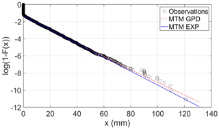
Figure 4 Exponential (EXP) probability plot of empirical and fitted cumulative distribution functions of daily rainfall depths collected at the Gioi Cilento weather station.

For each scenario pertaining to either the static or dynamic approach, we generated 10 000 equiprobable realizations of synthetic daily rainfall time series, each 3 years long, according to a stochastic Poisson point process model. In each modeling scenario, the synthetic time series was then used as input for the SWAT model to evaluate the effects on the water balance components in UARC. As anticipated in Sect. 3, the first 2 years represent warmup simulations and were thus discarded, while only results for the third year were stored for subsequent analyses presented in the next section.

To further evaluate the hydrologic behavior of the study catchment, an issue deserving more detailed attention is the assessment of the sensitivity of water balance to rainfall seasonality. With this aim, we refer to the Budyko framework (Budyko, 1974), which has been extensively applied to relate water components in different climatic contexts worldwide, including the Mediterranean climate (see, e.g., Viola et al., 2017; Caracciolo et al., 2017). Specifically, the Budyko framework relates the evaporative index (ET_a∕R) to the dryness index (ET_p∕R) computed at an annual timescale in terms of “available water” (i.e., rainfall R). Potential evapotranspiration ET_p is limited by either energy supply (for the dryness index less than or equal to one) or water supply (for the dryness index greater than one), and therefore the Budyko space has two physical bounds dictated by either the atmospheric water demand (ET_a≤ET_p) or the atmospheric water supply (ET_a≤R). The first bound is the energy limit (or demand limit, i.e., the 1:1 line corresponding to ET_a= ET_p) implying that actual evapotranspiration cannot exceed potential evapotranspiration. The second bound is the water limit (or supply limit, i.e., the horizontal line corresponding to ET_a=R) implying that actual evapotranspiration cannot exceed precipitation when the dryness index is greater than one (i.e., ET_p∕R > 1).

5 Results and discussion

5.1 Static approach for assessing rainfall seasonality

The observed temporal evolution of SPI-6 in our 90-year time series (see gray bars in Fig. 5) highlights prolonged droughts amongst the 1980s and 1990s and prolonged wet periods in the last decade when SPI-6 values above the threshold +2 occurred in 2008, 2010, and 2012. Yet, by splitting the SPI-6 values into two 45-year subgroups, we can observe that the last 45-year period is characterized by a drier climate compared to the first 45-year period. Specifically, in the first subgroup the probabilities of obtaining SPI-6 > +1 and SPI-6 < −1 are 17.9 % and 7.6 %, respectively. In contrast, in the second subgroup there is a general increase in negative SPI-6 values: the probability of obtaining SPI-6 > +1 becomes 11.9 %, and that of obtaining SPI-6 < −1 is 19.3 %. By analyzing daily rainfall datasets recorded at 55 weather stations located in the region of Basilicata near UARC (characterized by similar climatic conditions), Piccarreta et al. (2013) observed a general decreasing trend in the mean annual rainfall over the period of 1951–2010 mainly due to the autumn–winter decrease in precipitation.

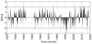
Figure 5 Temporal evolution of SPI-6 spanning from 1920 to 2018 (rainfall data were recorded at the Gioi Cilento weather station).

We now discuss the results pertaining to the calculation of the seasonal pattern of SPI-1 values. Rainfall seasonality under a Mediterranean climate can be assumed to be roughly represented by the alternation of two 6-month seasons, characterized by positive and negative SPI-1 values (wet and dry season, respectively; Rivoire et al., 2019). The temporal evolution of the SPI-1 values is represented by the gray bars in Fig. 6a and highlights the seasonal cycle within each year, whereas their 12-month moving average (magenta line in Fig. 6a) oscillates around the zero value with prolonged dry periods during the 1980s and 1990s and prolonged wet periods in the 2000s and 2010s. Figure 6b shows the box and whiskers plots of the SPI-1 values for each month of the year, thus depicting the monthly distribution of this index throughout the available recorded period. The median SPI-1 values (central red line in the blue boxes) are negative only from May to August and positive from September to April, even though the whiskers (identified by the two lines at the 25th and 75th percentile) denote the presence of relatively large variability in almost all months. Closer inspection of this graph enables one to identify three main seasonal features: (i) a dry period from May to August with median values below zero, (ii) a rainy period from November to February with median values above zero, and (iii) two transition periods from wet to dry (March and April) and from dry to wet (September and October) with median values near zero. We are aware that the median values in March, April, and October of the transition season are above zero, rather than “near” zero, but we recall that the Mediterranean climate in UARC is subhumid mainly due to orographic influences. However, this approach is intrinsically a “static” procedure, since the subdivision of the 12 months into three groups is rigid even though months in the transition periods have high variability in SPI-1 values. This outcome refines the initial working hypothesis of seasonal alternation of two semesters.

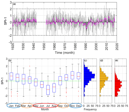
Figure 6 (a) Temporal evolution of SPI-1 values (gray bars) and their 12-month moving average (magenta line) spanning from 1920 to 2018 in the static approach. (b) Box plots of SPI-1 values and the frequency distribution in the (c) rainy period (blue histograms corresponding to November–December–January–February), (d) transition period (yellow histograms corresponding to March–April–September–October), and (e) dry period (red histograms corresponding to May–June–July–August).

The frequency distributions of the SPI-1 values computed over the rainy, dry, and transition seasons are illustrated in Fig. 6c–e. The wet season (depicted by the blue histograms) is characterized by probabilities having SPI-1 values greater than 0, +1, +2, and +3 of 80.60 %, 30.50 %, 1.90 %, and 0.30 %, respectively. The dry season (depicted by the red histograms) is associated with SPI-1 values lower than 0, −1, −2, and −3 with probabilities of 78.10 %, 31.10 %, 0.56 %, and 0.10 %, respectively. Conversely, we warn that probabilities of obtaining positive SPI-1 values in the transition season are 63.30 % instead of the expected 50 % if the hypothesis were “perfectly true”. Therefore, we considered three different scenarios, each with fixed and recurrent alternation of seasons during the hydrological year: (i) a “reference scenario” with a 4-month wet season (November, December, January, and February – NDJF), a 4-month dry season (May, June, July, and August – MJJA), and a 4-month transition season (March and April – MA – from wet to dry and September and October – SO – from dry to wet); (ii) a “dry scenario”, which mimics an extreme drought anomaly, characterized by a prolonged 8-month dry season (from March to October) and abrupt alternations with the 4-month wet season (NDJF), without any transition season; and (iii) a “wet scenario”, which mimics an extremely rainy anomaly, characterized by a prolonged 8-month wet season (from September to April) and abrupt alternations with the 4-month dry season (MJJA), again with no transition season.

In light of the above results, the two Poisson parameters (η and λ) describing daily rainfall values were calculated for each of the three seasons in the reference scenario and were then also used to develop synthetic simulations of rainfall time series in the dry and wet scenarios (see Table 2).

Table 2 Scenario setup in the static approach. Duration and Poisson distribution parameters (η and λ) are reported for each of the considered scenarios.

5.2 Dynamic approach for assessing rainfall seasonality

The centroid of the monthly rainfall distribution measured at the Gioi Cilento weather station (in the 90 years between 1920 and 2018) indicates that the wet season is centered in the second half of December, while its average duration is about 5.44 months (see Fig. 7). Nonetheless, it is worth noting the occurrence of a few extreme situations: the severe drought recorded in 1985 caused a minimum duration of about 4 months of the rainy period, while the year 1964 registered a maximum duration of about 7.0 months. The term “dynamic” used for this approach stems mainly from the fact that the duration of the rainy period is time variant throughout the years.

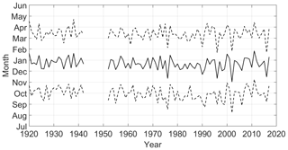
Figure 7 Temporal evolution of the centroid (or timing; solid line) and spread (or duration; dashed lines) of the wet seasons estimated as proposed by Feng et al. (2013) within the framework of the dynamic approach (rainfall data were recorded at the Gioi Cilento weather station).

The dimensionless seasonality index (DSI) and the seasonality index (SI) were computed for the Gioi Cilento time series according to procedures proposed by Feng et al. (2013) and by Walsh and Lawler (1981), respectively. The Mann–Kendall nonparametric test (Mann, 1945; Kendall, 1975) was then applied to evaluate the possible decreasing, increasing, or absence of temporal trends on these indexes and revealed that the null hypothesis of the absence of trend cannot be neglected at the 0.05 significance level for both indexes. The stationarity in time of the DSI (red line) and SI (green line) is also apparent from a perusal of Fig. 8, where the linear regressions (dashed and dotted for the DSI and SI, respectively) are characterized by very weak downward slopes.

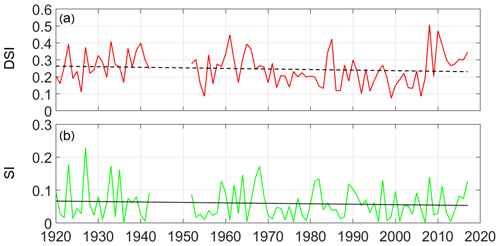
Figure 8 Temporal evolution of (a) dimensionless seasonal index (DSI; Feng et al., 2013) represented by a red line with a corresponding linear regression (dashed line). (b) Seasonality index (SI; Walsh and Lawler, 1981) represented by a green line with a corresponding linear regression (dotted line).

As described in Sect. 4.2, the dynamic approach assumes the alternation of only two seasons (wet and dry) with random durations of the rainy period. Figure 9a shows the time series of the 90 durations of the wet season estimated with the procedure proposed by Feng et al. (2013), while their frequency distribution is plotted in Fig. 9b. We then applied the Lilliefors statistical test (Lilliefors, 1967) to the null hypothesis of normality for the estimated wet durations obtaining a p value of 0.327, meaning that the null hypothesis cannot be rejected with the commonly adopted 5 % significance level. For each hydrological year, we thus generate a duration of the wet season from a normal distribution with the same mean and standard deviation of the Gioi Cilento time series (with a mean of 2.71 months and standard deviation of 0.28 months), while the dry seasons were consequently obtained as the complement in the same year to the wet seasons. In this case, the two Poisson parameters (η and λ) for modeling daily rainfall values were computed for the wet and dry seasons (Table 3).

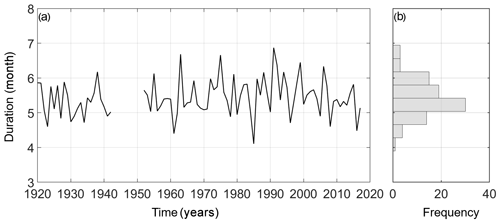
Figure 9 Time series (a) and frequency distribution (b) of durations of the rainy periods at the Gioi Cilento weather station in the dynamic approach.

Table 3 Scenario set up in the dynamic approach. Duration and Poisson distribution parameters (η and λ) are reported in the dry and wet seasons.

5.3 Effects of seasonal-rainfall anomalies on water balance when using the static approach

The results obtained from the three scenarios pertaining to the static approach are presented using the descriptive statistics of the water balance components at the annual timescale obtained from 10 000 SWAT simulation runs (Table 4). The reference scenario represents the normal situation with three seasons (dry, transition, and wet). Even though the range of annual rainfall values is relatively large, the coefficient of variation (CV) is only 14 %, implying that very low and very high annual rainfall depths (outliers) occur occasionally. The water balance components, namely water yield (WY), actual evapotranspiration (ET_a), and groundwater recharge (GR), represent on average 35 %, 49 %, and 16 % of the annual mean rainfall depth (R=1229 mm). The annual rainfall depths for the other two scenarios (only two seasons without the transition season) shift down to 988 mm (dry scenario) and up to 1393 mm (wet scenario), thus affecting the water balance. When the dry season lasts 8 months (dry scenario), water yield, actual evapotranspiration, and groundwater recharge decrease by 116, 60, and 66 mm, respectively, when compared to the reference scenario.

Table 4 Descriptive statistics of annual water balance components obtained in the three scenarios in the static approach. Units are in millimeters, except for CV (%). SD: standard deviation; CV: coefficient of variation.

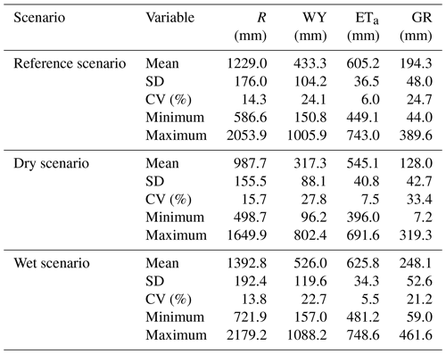
In contrast, when the wet season lasts 8 months (wet scenario), the water yield, actual evapotranspiration, and groundwater recharge increase by 93, 21, and 54 mm, respectively, when compared to the reference scenario. Water yield, actual evapotranspiration, and groundwater recharge represent on average 32 %, 55 %, and 13 % of the annual rainfall depth in the extreme dry season (dry scenario) and 38 %, 45 %, and 18 % of annual rainfall depth in the extreme wet season (wet scenario).

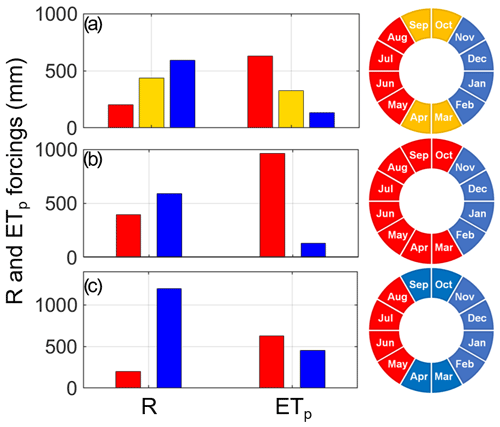
Figure 10 Rainfall and potential evapotranspiration forcings in the static approach, namely seasonal rainfall (R) and potential evapotranspiration (ET_p) in the dry (red bars), transition (orange bars), and wet seasons (blue bars). Three scenarios are presented: (a) reference scenario with the dry, transition, and wet seasons all lasting 4 months; (b) dry scenario with the dry and wet seasons lasting 8 and 4 months, respectively; and (c) wet scenario with the dry and wet seasons lasting 4 and 8 months, respectively.

Decomposition of the annual results into the seasonal components highlights other interesting features that are shown in Fig. 10 (rainfall and potential evapotranspiration forcings) and in Fig. 11 (main water balance components). For the reference scenario, the seasonal-rainfall depth is 201 mm, 436 mm, and 593 mm for the dry, transition, and wet seasons, respectively, representing 16 %, 35 %, and 48 % of the total annual rainfall (see Fig. 10a). Water yield depths span from 44 mm during the dry season to 251 mm during the rainy season (see Fig. 11a). Almost 60 % of annual water yield occurs over the wet season; about 30 % occurs in the transition season; and about 10 % occurs in the dry season. In contrast, the actual evapotranspiration depths are higher than rainfall depths in the dry season (269 mm) and lower than rainfall depths during the transition (226 mm) and rainy (110 mm) seasons (see Fig. 11a).

Over the dry scenario (see Figs. 10b and 11b), the months belonging to the transition season become drier than normal. The total rainfall depths over the dry and wet seasons are 397 mm and 590 mm, respectively, whereas the extreme drought anomaly induces precipitation loss only in the dry season with a considerable decrease of 239 mm of rainfall depth (Fig. 10b). The consequences of this situation on the average water balance components in the prolonged dry season lead to significant deficits (Fig. 11b). Water yield loss over the dry season is 93 mm, which represents 50 % of water yield obtained for the dry and transition seasons in the reference scenario. The wet season (from November to February) provides about 590 mm of water yield per year. The water loss by actual evapotranspiration is limited and represents only 10 % of ET_a obtained for the dry and transition seasons in the reference scenario (Fig. 11b).

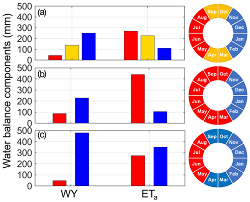
Figure 11 Main water balance components in the static approach, namely seasonal water yield (WY) and actual evapotranspiration (ET_a) in the dry (red bars), transition (orange bars), and wet seasons (blue bars). Three scenarios are presented: (a) reference scenario with the dry, transition, and wet seasons all lasting 4 months; (b) dry scenario with the dry and wet seasons lasting 8 and 4 months, respectively; and (c) wet scenario with the dry and wet seasons lasting 4 and 8 months, respectively.

In the wet scenario (see Figs. 10c and 11c), the months belonging to the transition season become wet (8 wet months and 4 dry months). Total rainfall depths in the dry and wet seasons are 200 mm and 1193 mm (Fig. 10c). Rainfall depth increases by 164 mm in the wet season (+14 % compared with that obtained in the wet and transition seasons in the reference scenario). Water yield gain in the wet season is 89 mm, which represents 20 % of water yield obtained in the wet and transition seasons in the reference scenario (Fig. 11c). The water lost by actual evapotranspiration is negligible.

5.4 Effects of seasonal-rainfall anomalies on water balance when using the dynamic approach

The second approach to assessing the effect of rainfall seasonality extremes on water balance components is based on the stochastic generation of the wet-season durations from their normal distribution (see Fig. 9b). This approach helps classify the results within a probabilistic framework according to the following rainy period duration classes: 3–4, 4–5, 5–6, 6–7, and 7–8 months. Seasonal extremes (3–4 and 7–8 months) have very low probabilities of occurrence (0.60 % and 0.30 %, respectively). Nonetheless, it is interesting to analyze the effect of rainfall variability on water yield (WY), actual evapotranspiration (ET_a), and groundwater recharge (GR). The most probable (62 %) situation occurs when the rainy period lasts 5–6 months. Under these circumstances, the mean annual rainfall depth is 1275 mm, whereas WY, ET_a, and GR represent 35 %, 49 %, and 16 % of annual average rainfall depth, respectively. These percentages are very close to those observed in the reference scenario of the static approach. If the wet season shortens by 1 month (23 % probability), the mean annual rainfall depth decreases by 62 mm, whereas water yield depth changes by 33 mm (−7 %). In contrast, if the wet season is made up of 6–7 months (14 % probability), the annual mean rainfall depth increases by 51 mm, and water yield changes by 27 mm (+6 %).

Extremely dry and extremely wet situations reflect similar results obtained from the dry and wet scenarios presented above. A prolonged drought (i.e., rainy period of only 3–4 months long) leads to an average rainfall loss of 130 mm per year inducing an appreciable annual decrease in both water yield (−68 mm) and groundwater recharge (−30 mm). A prolonged wet season (i.e., lasting 7–8 months), instead, causes average rainfall to gain approximately 108 mm per year, yielding annual increases in both water yield (+59 mm) and groundwater recharge (+12 mm). It is worth noting that the duration of the rainy period does not seem to exert a major control on the water balance. Pearson's linear correlation coefficients between duration and average annual rainfall, water yield, and actual evapotranspiration are 0.22, 0.20, and 0.11, respectively.

Table 5 Water balance components associated to occurrence probabilities for each duration of the rainy period.

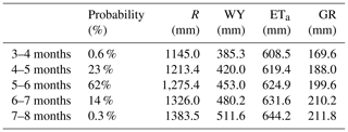
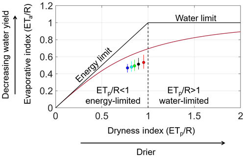
Figure 12 Budyko diagram relating the dryness index (ET_p∕R) with the evaporative (ET_a∕R) index classified according to the duration of the rainy period pertaining to the dynamic approach. Circles denote the median and vertical colored lines represent the range between the 5th and 95th percentiles of the evaporative index (red, black, green, cyan, and blue correspond to the duration of the rainy period of 3–4, 4–5, 5–6, 6–7 and 7–8 months, respectively). Solid lines denote energy and water limits; the solid garnet line represents the Budyko curve (Budyko, 1974). The vertical dashed line separates the left-hand side from right-hand side of the Budyko curve.

Assuming that the long-term mean annual precipitation can be partitioned into the mean annual actual evapotranspiration and mean annual water yield, according to the Budyko framework we assume that larger values of the dryness index (drier climate conditions; ET_p∕R > 1) induce a greater proportion of rainfall that is partitioned to ET_a. In contrast, data on the left-hand side of the Budyko curve will be characterized by a greater proportion of rainfall that is partitioned to water yield. Fig. 12 shows the Budyko plot of the dryness index (ET_p∕R) versus the evaporative index (ET_a∕R) together with the Budyko curve (solid garnet line). In this plot we depict the data points (colored dots) for the five different durations of the rainy period in UARC obtained by the dynamic approach. The first comment to be made is that all of these data points gather within the energy-limited region of the Budyko plot, with the longest rainy period (blue dot) favoring conditions of greater discharges (evaporative index ET${}_{\mathrm{a}}/R=\mathrm{0.45}$) and the shortest rainy period (droughts indicated by the red dot) inducing higher evapotranspiration fluxes (evaporative index ET${}_{\mathrm{a}}/R=\mathrm{0.54}$). The latter situation shows that on average the upper Alento River catchment is characterized by relatively good storage of soil water made possible by the hydraulic properties of the soils and the large portion of shrub spots and forest areas (mostly deciduous chestnut forests and olive orchards), together with a good amount of annual precipitation in a hilly and mountainous zone in southern Italy. However, it may also be noted that all of these data points cluster below the Budyko curve (Williams et al., 2012). The observed departure below the Budyko curve may be due to several reasons. Allowing for the Budyko assumptions for water balance, the present study refers to a long timescale (90 years) but a relatively small spatial scale, since UARC has a drainage area of 102 km². In fact, rainfall seasonality (i.e., intra-annual variability) may be just one of the major factors that could have led to a departure from the Budyko curve. The typical Mediterranean climate, which is characterized by precipitation being out of phase with potential evapotranspiration, is also singled out as a cause of the deviations we observed in our case study from the Budyko curve (Milly, 1994). Normal situations, characterized by a wet season lasting 5–6 months (green dot), lead to rainfall being partitioned into 49 % ET_a, as indicated by the evaporative index value of 0.49. We hereby recall that this study is based on the assumption that the catchment response is not affected by human interferences and their feedbacks (land use change, change in soil hydraulic properties, enhanced evapotranspiration induced by global warming, etc.) but only by changes in rainfall seasonality which, of course, can undermine Budyko's implicit assumption of a temporal steady state (Feng et al., 2012; Troch et al., 2013).

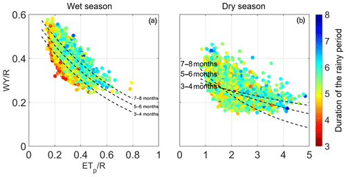
Figure 13 Relationship between the dryness index and water yield to rainfall ratio (WY ∕ R) on a seasonal basis and classified according to the duration of the wet season (from shortest to longest denoted by reddish and bluish colors in the color bar) pertaining to the dynamic approach for the wet season (a) and the dry season. The exponential-regression equations are represented in both plots by the dashed black lines according to the duration of the rainy period.

Table 6 Exponential-regression models, with the corresponding coefficient of determination (R²), for the wet and dry seasons as a function of the duration of the rainy period.

The relationships between the seasonal dryness index and the ratio of water yield to rainfall (WY ∕ R) are affected by the duration of the wet season and are depicted in Fig. 13. The coefficients of the exponential-regression models with their corresponding R² values pertaining to the wet or dry season are reported for each duration class of the rainy period in Table 6. The exponential curves in the wet season (see Fig. 13a) are virtually parallel, yielding, for a fixed ET_p∕R value, a higher WY ∕ R value as the duration of the rainy period increases from 3–4 to 7–8 months. In contrast, the exponential-regression curves belonging to the dry season (see Fig. 13b) explain only a small amount of the variations of WY ∕ R in response to the dryness index and all seem quite insensitive to rainfall seasonality. Only the exponential model pertaining to the dry season and for the smaller duration of the rainy period (3–4 months) explains slightly less than 50 % of the variability of ET_p∕R for the study catchment.

6 Conclusions

Capturing the relationship between precipitation and catchment-scale water balance components in a Mediterranean context is a scientific challenge in view of expected increasing frequencies in extremes such as droughts and floods induced by climate warming. On the one hand, intense and prolonged droughts induce a steep decline in water availability for irrigation (with a subsequent decrease in crop productivity), domestic use (especially for the tourist sector), and clean power generation to mention just a few. On the other hand, projected increments in runoff and flooding induce a higher-than-normal risk of landslides and soil erosion, compromising the local economy and leading to unprecedented hazards for a vulnerable population. Therefore, countries across the Mediterranean region are being forced to pursue drastic adaptive options which in turn depend on modeling scenarios which can be performed by using hydrological models. Indeed, scenarios need to rely on adequate rainfall modeling within the hydrological year by generating multiple datasets of reliable daily rainfall time series drawn from statistical distributions derived from long-term observations. Nonetheless, a key is first to define rainfall seasons and then optimize parameters featuring in the best statistical distribution describing the rainfall data distribution in each season. If this exercise is well posed, one can capture realistic rainfall dynamics occurring in the water balance simulated by a numerical model. Within this framework, the aim of this study is to contribute to understanding the impact of rainfall seasonality and its anomalies on the water balance components by providing reliable and robust scenario-based projections, based on the use of well-posed hydrological models.

This study presented a pilot area (UARC in southern Italy) in the Mediterranean region. We applied the SWAT model that was calibrated and validated in a previous paper using a large amount of environmental data and maps (Nasta et al., 2017). Moreover, the availability of a long-term time series of daily rainfall data (almost 1 century) allowed us to detect rainfall seasonality by using a static and a dynamic approach. In both approaches we apply the SWAT model to evaluate the sensitivity of hydrological water balance components to rainfall seasonality, using as input synthetic rainfall time series generated by a Poisson process with two parameters that characterize daily rainfall occurrences and daily rainfall depth in each season. In the static approach, dry or wet anomalies are considered when the transition seasons turn into dry or wet seasons. The advantage of this approach lies in its simplicity and easy reproducibility in other sites. However, it can be considered only an artifact based on criteria to group monthly rainfall amounts that might be subjective. In the dynamic approach, the seasonal anomalies occur on the tails of the normal distribution of the wet-season duration. Although this approach seems statistically sound, the main disadvantage is the fact that it requires long-term historical rainfall time series of daily rainfall data that are unlikely to be available in most weather stations across the Mediterranean region. In this study, both approaches concurred on understanding the impact of seasonal-rainfall anomalies on catchment-scale water balance components.

Our results show that a drought anomaly (i.e., a prolonged duration of the dry season) in just a single year potentially leads to a decrease of even about a fifth of the annual average rainfall and induces a drastic decline in average annual amounts of water yield, actual evapotranspiration, and groundwater recharge. Conversely, an exceptionally prolonged wet season is likely to cause a considerable increase in annual average rainfall, hence about a one-third rise in annual average water yield as well as enhanced groundwater recharge. In the dynamic approach, we demonstrated that the implicit assumption of a temporal steady state in the Budyko relation approach is sensitive to rainfall seasonality. The Budyko evaporative index spans from 0.45 to 0.54 when the wet season lasts from 7–8 months to 3–4 months. Moreover, it is possible to identify distinct season-dependent regression equations linking seasonal water yield to the dryness index over the wet season.

In conclusion this paper provides a framework to analyze the effects of rainfall seasonality changes on the hydrological water budget and partition while providing some preliminary results that can be representative for Mediterranean catchments. Finer analyses can be performed by considering consecutive years of prolonged drought episodes and/or by adding the effects of temperature trends, which obviously affect potential evapotranspiration forcing and in principle can produce a further feedback on precipitation cycles. These still-unexplored issues will form the subject of future research investigations and forthcoming reports.

Appendix A

We set k and m as counters for the hydrological year and the 12 months in each year, respectively. The annual rainfall R_k and associated monthly probability distribution p_k,m are defined as

$$\begin{array}{}\text{(A1)}& {\displaystyle }{R}_k=\sum _{m=\mathrm{1}}^{\mathrm{12}}{r}_{k,m},\text{(A2)}& {\displaystyle }{p}_{k,m}={\displaystyle \frac{r_{k,m}}{R_k}},\end{array}$$

where r_k,m represents the rainfall depth recorded in the mth month of the kth year.

The relative entropy D_k is calculated in each hydrological year k as

$$\begin{array}{}\text{(A3)}& D_k=\sum _{m=\mathrm{1}}^{\mathrm{12}}{p}_{k,m}{\log }_{\mathrm{2}}\left({\displaystyle \frac{p_{k,m}}{q_m}}\right),\end{array}$$

where q_m is equal to 1∕12 (uniform distribution). This statistical index quantifies the distribution of monthly rainfall within each hydrological year. Finally, the dimensionless seasonality index (DSI_k) in each hydrological year k is given by

$$\begin{array}{}\text{(A4)}& {\mathrm{DSI}}_k=D_k{\displaystyle \frac{R_k}{{\stackrel{\mathrm{‾}}{R}}_{\max }}},\end{array}$$

where ${\stackrel{\mathrm{‾}}{R}}_{\max }$ is the maximum $\stackrel{\mathrm{‾}}{R}$ value. This way DSI_k is zero when rainfall is uniformly distributed throughout the year and reaches its maximum value of log₂12 when rainfall is concentrated in a single month.

According to Feng et al. (2013), the magnitude (R_k) represents annual rainfall, whereas the centroid (C_k) and the spread (Z_k) indicate timing and duration of the wet season, respectively, and are calculated in each hydrological year k as

$$\begin{array}{}\text{(A5)}& {\displaystyle }{C}_k={\displaystyle \frac{\mathrm{1}}{R_k}}\sum _{m=\mathrm{1}}^{\mathrm{12}}m{r}_{k,m},\text{(A6)}& {\displaystyle }{Z}_k=\sqrt{{\displaystyle \frac{\mathrm{1}}{R_k}}\sum _{m=\mathrm{1}}^{\mathrm{12}}{\left|m-C_k\right|}^{\mathrm{2}}{r}_{k,m}}.\end{array}$$