the Creative Commons Attribution 4.0 License.
the Creative Commons Attribution 4.0 License.
 | 17 Jun 2020
Crossing hydrological and geochemical modeling to understand the spatiotemporal variability of water chemistry in a headwater catchment (Strengbach, France)
Julien Ackerer
Benjamin Jeannot
Frederick Delay
Sylvain Weill
Yann Lucas
Bertrand Fritz
Daniel Viville
François Chabaux
Understanding the variability of the chemical composition of surface waters is a major issue for the scientific community. To date, the study of concentration–discharge relations has been intensively used to assess the spatiotemporal variability of the water chemistry at watershed scales. However, the lack of independent estimations of the water transit times within catchments limits the ability to model and predict the water chemistry with only geochemical approaches. In this study, a dimensionally reduced hydrological model coupling surface flow with subsurface flow (i.e., the Normally Integrated Hydrological Model, NIHM) has been used to constrain the distribution of the flow lines in a headwater catchment (Strengbach watershed, France). Then, hydrogeochemical simulations with the code KIRMAT (i.e., KInectic Reaction and MAss Transport) are performed to calculate the evolution of the water chemistry along the flow lines. Concentrations of dissolved silica (H4SiO4) and in basic cations (Na+, K+, Mg2+, and Ca2+) in the spring and piezometer waters are correctly reproduced with a simple integration along the flow lines. The seasonal variability of hydraulic conductivities along the slopes is a key process to understand the dynamics of flow lines and the changes of water transit times in the watershed. The covariation between flow velocities and active lengths of flow lines under changing hydrological conditions reduces the variability of water transit times and explains why transit times span much narrower variation ranges than the water discharges in the Strengbach catchment. These findings demonstrate that the general chemostatic behavior of the water chemistry is a direct consequence of the strong hydrological control of the water transit times within the catchment. Our results also show that a better knowledge of the relations between concentration and mean transit time (C–MTT relations) is an interesting new step to understand the diversity of C–Q shapes for chemical elements. The good match between the measured and modeled concentrations while respecting the water–rock interaction times provided by the hydrological simulations also shows that it is possible to capture the chemical composition of waters using simply determined reactive surfaces and experimental kinetic constants. The results of our simulations also strengthen the idea that the low surfaces calculated from the geometrical shapes of primary minerals are a good estimate of the reactive surfaces within the environment.
- Article
(7177 KB) - Full-text XML
-
Supplement
(618 KB) - BibTeX
- EndNote


Understanding the effects of ongoing climatic changes on the environment is a major issue for the coming years. The global increase in temperature is expected to affect the hydrological cycle at a large scale, and providing a precise estimation of its repercussions for the evolution of soils and for the chemistry of waters remains difficult. This challenge results from the wide diversity of hydrological, geochemical and biological processes, and of their coupling, which operate at the Earth's surface (e.g., Gislason et al., 2009; Goddéris et al., 2013; Beaulieu et al., 2012, 2016). Up until today, the study of concentration–discharge relations (C–Q relations) has been intensively used to assess the coupling between hydrological and geochemical processes at the hillslope or watershed scales (Godsey et al., 2009; Kim et al., 2017; Ameli et al., 2017; Diamond and Cohen, 2018).
C–Q relations are acknowledged to integrate critical zone structure, the hydrological dynamics and the geochemical processes of watersheds (Chorover et al., 2017). Recent studies debated the extent to which the chemical variability of waters is explained by a mixing of different water sources (Zhi et al., 2019), the chemical contrasts between deep and shallow waters (Kim et al., 2017), the variability in transit times (Ackerer et al., 2018), and/or seasonally variable flow paths (Herndon et al., 2018). It is clear that a good knowledge of the water flow paths and of their seasonal variability is an important new step to better constrain the water transit times within catchments, and then to correctly understand the temporal fluctuations of the composition of waters. Modeling such variability of water flow paths and water geochemical composition would require further development of modeling approaches able to combine hydrological and geochemical processes (e.g., Steefel et al., 2005; Kirchner, 2006).
Recent efforts in hydrological modeling were conducted to develop spatially distributed approaches that better consider the interplay between surface and subsurface processes (e.g., Gunduz and Aral, 2005; Kampf and Burges, 2007; Camporese et al., 2010). Due to the complexity of flows in the hydrological processes, many modeling approaches are based on the full resolution of Richard's and Saint-Venant equations to correctly describe the interactions between stream, overland and subsurface waters (Kampf and Burges, 2007). These approaches have shown their ability to capture the hydrological functioning of various watersheds, knowing that the full resolution of Richard's and Saint-Venant equations requires long computational times and faces calibration and parameterization difficulties (Ebel and Loague, 2006; Mirus et al., 2011). Questions have been raised regarding the optimal complexity of the equations that are needed to correctly treat the hydrology of catchments in their surface and subsurface compartments with reasonable computation times (Gunduz and Aral, 2005).
Low-dimensional models have attracted growing interest because they represent an interesting compromise between equation complexity, computational time and result accuracy (Pan et al., 2015; Hazenberg et al., 2016; Weill et al., 2013, 2017; Jeannot et al., 2018). The reduction of dimensionality is mainly associated with a subsurface compartment (including both the vadose and the saturated zones) modeled as a two-dimensional layer. Some low-dimensional models, such as the one employed in this study, can solve subsurface flow via an integrated Richard's equation, meaning that flow and transport processes are integrated over a vertical direction or a direction normal to bedrock, and manipulate averaged (integrated) hydrodynamic properties. This type of low-dimensional approach recently demonstrated its ability to reproduce the results from fully dimensioned approaches in small catchments while reducing computational costs (Pan et al., 2015; Jeannot et al., 2018). Nonetheless, the water transit times calculated from these depth-integrated models are rarely confronted with the water–rock interaction times inferred from hydrogeochemical modeling of water chemistry in watersheds.
For its part, the understanding of the hydrogeochemical functioning of the critical zone has been significantly advanced by the implementation of reactive-transport laws in geochemical modeling codes (Steefel et al., 2005; Lucas et al., 2010, 2017; Goddéris et al., 2013; Li et al., 2017a). These developments allow a variety of processes to be considered, such as flow and transport processes, ion exchanges, biogeochemical reactions, and the interplay between primary mineral dissolution and secondary mineral precipitation (Moore et al., 2012; Lebedeva and Brantley, 2013; Ackerer et al., 2018). Reactive transport models have been used to explore a wide variety of scientific issues, including the study of global atmospheric CO2 consumption by weathering reactions (Goddéris et al., 2013; Li et al., 2014), the formation and evolution of soil and regolith profiles (Maher et al., 2009; Navarre-Sitchler et al., 2009; Lebedeva and Brantley, 2013), and the variability of water quality and chemistry in the environment (Lucas et al., 2010, 2017; Ackerer et al., 2018). However, these approaches usually rely on a simple 1D flow path through a regolith column or along a hill slope to model flow in the system (e.g., Maher, 2011; Moore et al., 2012; Lucas et al., 2017; Ackerer et al., 2018). 1D reactive-transport models are useful to discuss the key processes involved in the regolith formation and in the acquisition of the water chemical composition, but these models cannot consider the complexity of the flow trajectories in watersheds, and hence, its effects on the water chemistry.
A new step is therefore necessary for the development of hydrogeochemical modeling approaches that are applicable at the watershed scale and are able to integrate the complexity of the water flows and the diversity of the water–rock interaction processes. Recent efforts have been undertaken in the direction of merging hydrological and geochemical codes, with, for example, the parallel reactive transport code ParCrunchFlow (Beisman et al., 2015), or the coupled hydrogeochemical code RT-Flux-PIHM (Bao et al., 2017; Li et al., 2017a). As an alternative to fully dimensioned codes, this work proposes an original low-dimensional approach, with relatively short computation times and applicable at the watershed scale. This study is combining for the first time in this manner the results from a hydrological low-dimensional (depth-integrated for the subsurface) but spatially distributed model (Normally Integrated Hydrological Model, NIHM) with a reactive-transport model (KIRMAT). The combination allows the flow trajectories, the flow rates, the weathering reactions and the evolution of the water chemistry within a headwater system, the Strengbach catchment, to be simulated over time and space.
This catchment is one of the reference observatories of the French critical zone network (OZCAR), where multidisciplinary studies, including hydrological, geochemical and geological investigations, have been performed since 1986 (“Observatoire Hydrogéochimique de l'Environnement”, OHGE; http://ohge.unistra.fr, last access: 15 June 2020; El Gh'Mari, 1995; Fichter et al., 1998; Viville et al., 2012; Gangloff et al., 2014, 2016; Prunier et al., 2015; Pan et al., 2015; Ackerer et al., 2016, 2018; Beaulieu et al., 2016; Chabaux et al., 2017, 2019; Schmitt et al., 2017, 2018; Daval et al., 2018; see also Pierret et al., 2018, for an updated overview of the Strengbach watershed).
The Strengbach catchment is a small watershed (0.8 km2) located in the Vosges Mountains of northeastern France at altitudes between 883 and 1147 m. Its hydroclimatic characteristics can be found in Viville et al. (2012) or in Pierret et al. (2018). It is marked by a mountainous oceanic climate, with an annual mean temperature of 6 ∘C and an annual mean rainfall of approximately 1400 mm, with 15 % to 20 % falling as snow during 2 to 4 months per year. The snow cover period is quite variable from year to year and may not be continuous over the entire winter. The annual mean evapotranspiration is approximately 600 mm, and the annual mean infiltration (no significant surface runoff observed) approximately 800 mm (Viville et al., 2012). The watershed is currently covered by a beech and spruce forest. The bedrock is a base-poor Hercynian granite covered by a 50 to 100 cm thick acidic and coarse soil. The granitic bedrock was fractured and hydrothermally altered, with a stronger degrees of hydrothermal overprinting in the northern than the southern part of the catchment (Fichter et al., 1998). The granite was also affected by surface weathering processes during the Quaternary (Ackerer et al., 2016). The porous and uppermost part of the granitic basement constitutes an aquifer from 2 to approximately 8 m thickness. In the Strengbach watershed, the major floods and high-flow events usually occur during snowmelt periods at the end of the winter season or in the early spring. By contrast, the low-flow periods commonly happen at the end of the summer or during the autumn. Several springs are captured for drinkable water supply directly in the subsurface by small collectors (Fig. 1). The watershed has been equipped with several piezometers and boreholes since 2012, those being located along the slopes on both sides of the watershed (Fig. 1 in Chabaux et al., 2017).
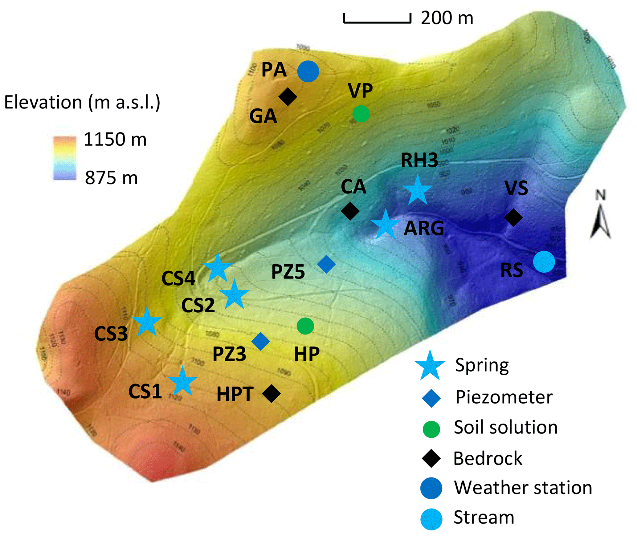
Figure 1Sampling locations within the Strengbach catchment. Blue stars represent springs, blue diamonds represent piezometers, and the blue circle represents the stream at the outlet of the watershed. Green circles represent soil solution locations, and black diamonds represent bedrock facies locations.
Spring waters have been regularly collected and analyzed since 2005, with monthly sampling supplemented by a few specific campaigns to cover the complete range of water discharges in the watershed. Piezometer waters have been collected only during specific sampling campaigns over the period 2012–2015, and, as for the spring waters, these sampling campaigns cover different hydrological conditions from wet to dry periods. The soil solutions were collected at a monthly frequency on the southern slope at a beech site (named HP) and to the north at a spruce site (named VP; Fig. 1; more details in Prunier et al., 2015). For all the collected waters, the concentrations of the major dissolved species and the pH were determined by following the analytical techniques used at LHyGeS (Strasbourg, France) and detailed in Gangloff et al. (2014) and Prunier et al. (2015). Discharges of water from the springs were measured during the sampling campaigns, as were the water levels within the piezometers.
The mineralogy and the porosity of the bedrock have been studied in detail in previous studies (El Gh'Mari, 1995; Fichter et al., 1998). On the southern part of the catchment, the weakly hydrothermally altered granite (named HPT; Fig. 1) is mainly composed of quartz (35 %), albite (31 %), K-feldspar (22 %) and biotite (6 %). It also contains small amounts of muscovite (3 %), anorthite (2 %), apatite (0.5 %) and clay minerals (0.5 %). On the northern part of the catchment, the lithology is more variable, with the presence of gneiss close to the crest lines and the occurrence of hydrothermally altered granite on the rest of the slopes (El Gh'Mari, 1995).
Table 1Measured pH, water discharges and chemical concentrations of H4SiO4, Na+, K+, Mg2+ and Ca2+ in water samples collected at the Strengbach catchment and used for the hydrogeochemical modeling. The sampling sites include springs (CS1, CS2, RH3) and piezometers (PZ3, PZ5).

The hydrological, geochemical and petrological data obtained from these field investigations are the basis of the modeling exercise presented in this study. More precisely, this study is based on hydrogeochemical data from 2005 to 2015 for waters from four springs in the southern part (CS1, CS2, CS3 and CS4) and one spring in the northern part (RH3) of the watershed (Fig. 1). Hydrogeochemical data obtained over the period 2012–2015 for two piezometers (PZ3, PZ5) in the southern part of the watershed are also studied (Fig. 1). The overall hydrogeochemical database is available as tables in the Supplement (Tables S1 to S9). The specific chemical data from spring and piezometer waters modeled in this study are reported in Table 1.
The modeling developments presented in this study represent a new step in the efforts undertaken to constrain the mechanisms controlling the geochemical composition of surface waters and to understand their spatial and temporal variations at the scale of headwater mountainous catchments (Schaffhauser et al., 2014; Lucas et al., 2017; Ackerer et al., 2018). The main innovation of this present work is to couple a spatially distributed and low-dimensional hydrological model with a reactive transport code to constrain the spatiotemporal variability of the chemical composition of waters. To the best of our knowledge, this is the first time that such a coupling between low-dimensional hydrological and hydrogeochemical modeling approaches has been attempted in this way at the watershed scale.
3.1 Hydrological modeling
To assess the water flows in the watershed, several simulations were performed with the hydrological code NIHM (Pan et al., 2015; Weill et al., 2017; Jeannot et al., 2018). This code is a coupled stream, overland and low-dimensional (depth-integrated) subsurface flow model developed at LHyGeS and already tested in the Strengbach watershed (Pan et al., 2015). The stream and overland flows are described by a diffusive-wave equation, and the subsurface flow is handled through an integration (in a direction normal to bedrock) of the unsaturated-saturated flow equation from the bedrock to the soil surface (Weill et al., 2017). The exchanges of water between the surface and subsurface flows are addressed via a first-order exchange coefficient involving the thickness and the hydraulic conductivity of an interface layer (e.g., the riverbed, for interactions between surface routing and subsurface compartments), and the hydraulic head differences between the compartments (Jeannot et al., 2018).
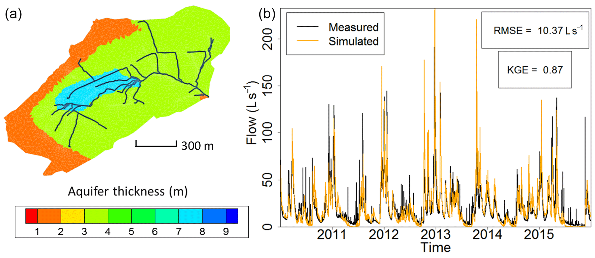
Figure 2(a) Calibrated field of thicknesses of the weathered material constituting the shallow unconfined aquifer at the Strengbach catchment used for the simulations by NIHM. The 1D surface draining network used in NIHM is represented by the black lines. The mesh for the groundwater compartment is represented by grey lines. (b) Fitting observed flow rates from the Strengbach stream at the outlet of the catchment with simulations of flow within the watershed (illustrated from 2010 to 2015). The subsurface compartment is inherited from the aquifer thicknesses reported in (a), and the topography lets the natural outlet of the subsurface compartment be the surface draining network.
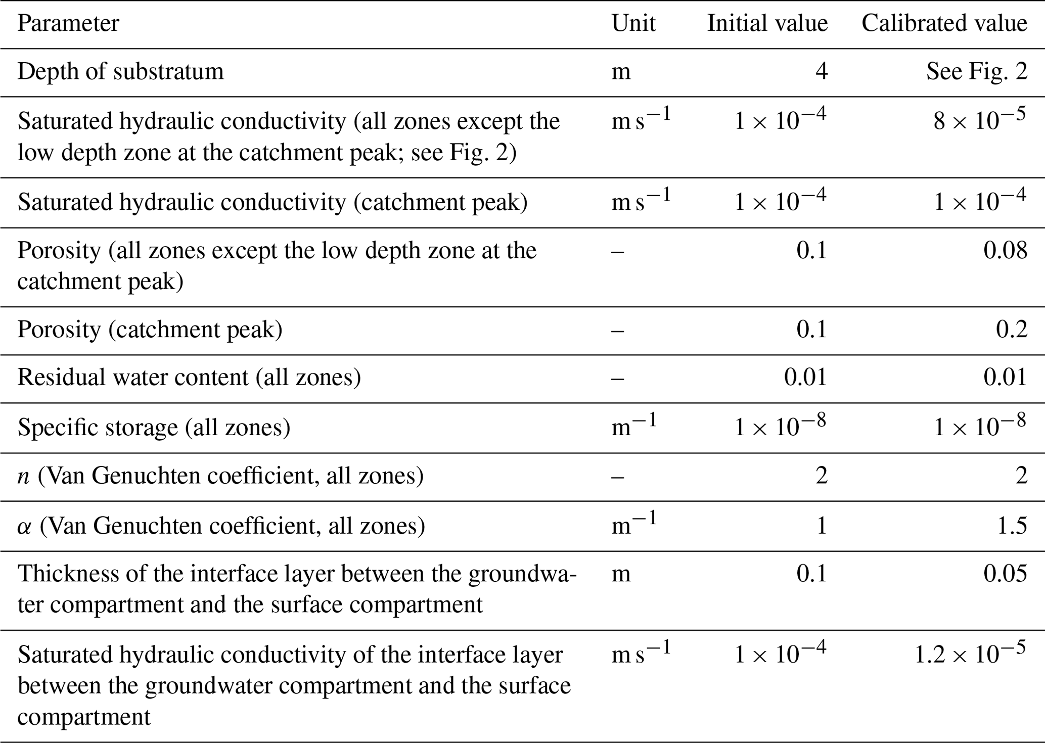
Regarding the hydrological simulations, NIHM was used with only its stream flow and subsurface flow compartments activated, the Strengbach catchment having never evidenced diffuse two-dimensional surface runoff or subsurface exfiltration over large areas. In addition, and because of the steep slopes, the stream flow process were revealed to be almost insensitive to the roughness and Manning's parameters of the riverbed, which were set to usual values for very small streams of mountainous landscapes. By contrast, the parameters of the subsurface were adjusted in NIHM through a calibration–validation process. Several zones of heterogeneity (Fig. 2) were defined based on field observations (Ackerer et al., 2016; Chabaux et al., 2017). In each of these zones, the saturated hydraulic conductivity, the depth of substratum and the porosity were set to uniform values. Other parameters (the residual water content, the specific storage, the Van Genuchten coefficients n and α, and the saturated hydraulic conductivity of the interface layer between the groundwater compartment and the surface compartment) were set to uniform values over the whole catchment (Table 2). The thickness of the aquifer that was used for the simulations varied from 2 m near the main crests to up to 8 m in the middle of the watershed (Fig. 2), in agreement with the data obtained during the recent geological investigations and drilling campaigns undertaken at the catchment (Ackerer et al., 2016; Chabaux et al., 2017). The uniform precipitation over space applied at the surface of the catchment are drawn from data of the pluviometric station located at the highest elevation of the watershed (site PA; Fig. 1). The hydrological model NIHM was then run over a first time period (years 1996–1997). Using a Monte Carlo approach, the parameters were “randomly” sought to improve the fitting between the observed and simulated flow rates at the outlet of the catchment (Table 2). The fit was quantified by the root mean square error (RMSE) and the Kling-Gupta efficiency coefficient (KGE; Gupta et al., 2009), applied to the outlet flow rate of the stream, which is the only reliable and always available hydrological variable monitored in the system.
Table 2Initial and calibrated values of the hydrodynamic parameters of the aquifer in the hydrological simulation of the Strengbach catchment by NIHM.
Once the best fit was obtained, the model was then run over another time period (2010–2015), but without changing the parameters anymore, and the quality of the fit was re-assessed for this new time period with the KGE and RMSE. Figure 2 shows the result for the 2010–2015 time period. After the water discharges were correctly reproduced at the outlet, a backtracking approach was used to identify which subsurface flow lines reach the sampled sites. To backtrack the water particles, the velocity fields calculated by the NIHM model were inverted in their direction, and the locations of the backtracked particles were saved at each time step. A daily time step was used for the backtracking, as a compromise between computational efforts and a refined description of the transient velocity fields. A schematic representation of the backtracking approach is given in Fig. 3. This methodology allows for constraining the flow lines that bring waters for a given time and at a given position on the catchment. This information is of major interest to determine the origin of the spring and piezometer waters. It is shown at the catchment scale that flows are mainly driven by gravity in association with the steep slopes of the watershed, the latter being almost evenly drained over its whole surface area (Fig. 4). For each water sampling area, 10 flow lines that bring water to the location of interest were determined (Fig. 4), together with a few features of the flow lines, including local velocities, mean velocities and length of the flow paths.
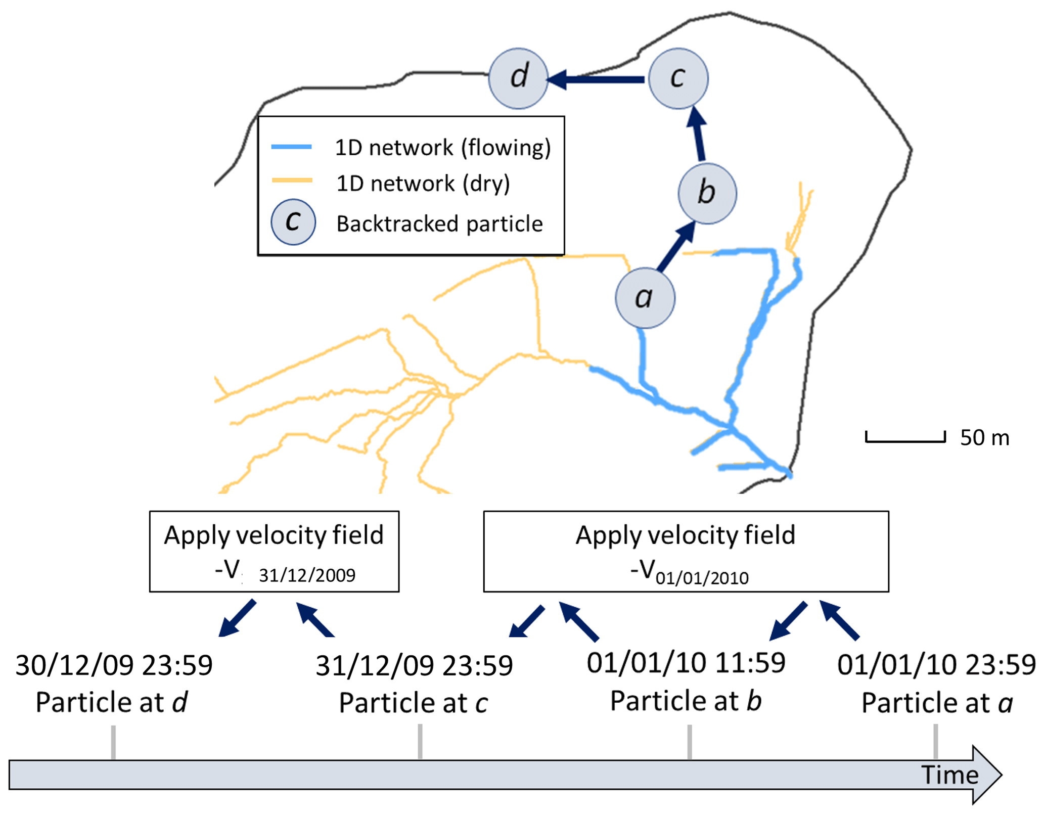
Figure 3Principle of the method of backtracking used to determine flow lines that generate flow at the outlet of the Strengbach catchment. Particles are dispatched along the wet fraction of the 1D river network (only one is represented here, at position a on 1 January 2010 at 23:59 GMT+1). NIHM generates an output heterogeneous velocity field on that date for the whole watershed, denoted V01/01/2010. By using a velocity field of the same magnitude but opposite direction to the particle, the position of the particle is backtracked until 31 December 2009 23:59 GMT+1. Then, to further backtrack the trajectory of the particle, the velocity field is updated accordingly. The frequency of velocity field updates is set to 1 d.
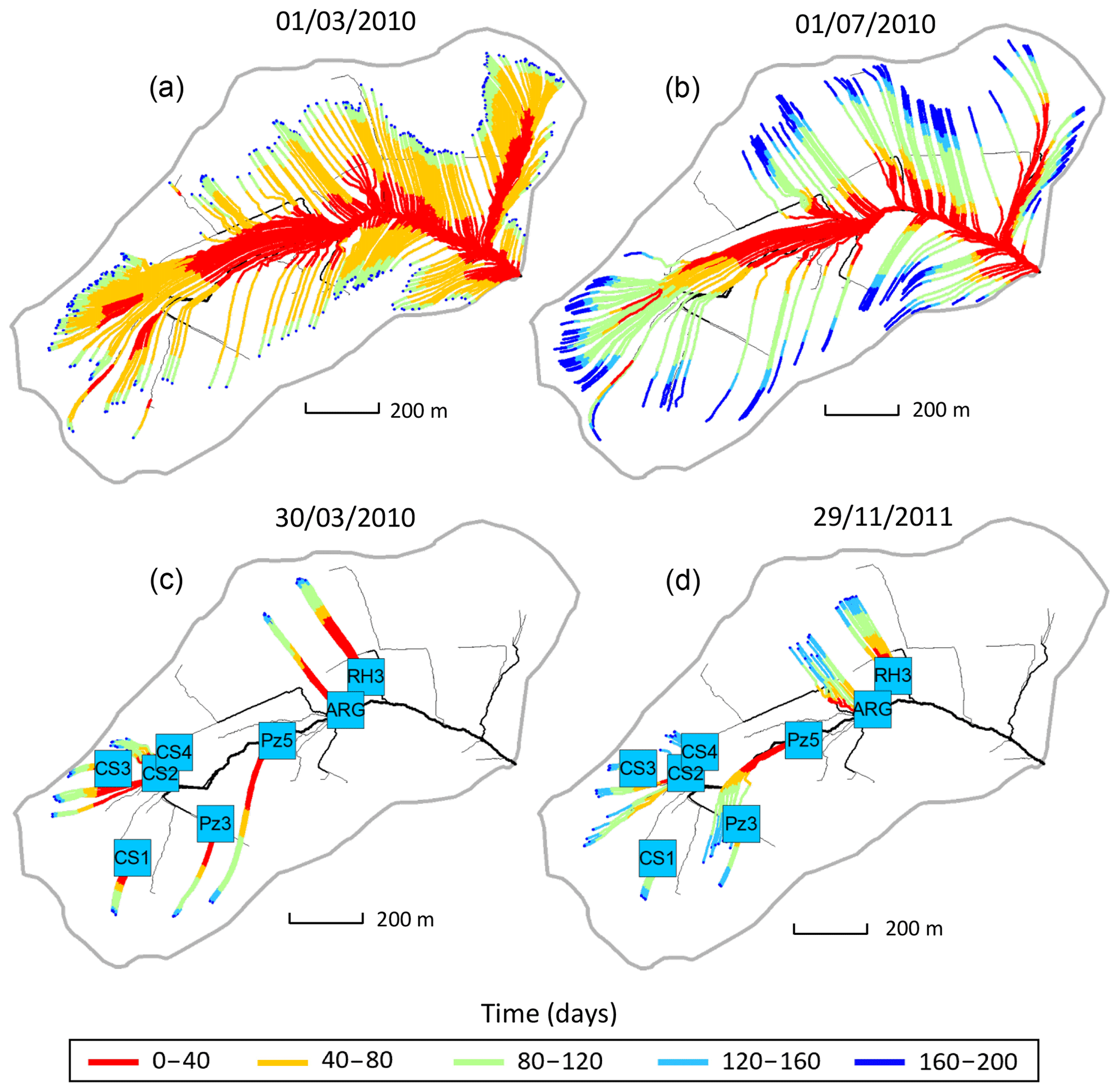
Figure 4(a, b) Flow lines of the subsurface that feed the surface draining network with water on 1 March 2010 (a, high-flow period) and 1 July 2010 (b, low-flow period). The color scale indicates that a water particle reaching the river at a given date started its travel along the streamline or passed at a given location on the streamline x days prior. The density of streamlines is associated with the flowing versus dry fraction of the river network at a prescribed date. (c, d) Flow lines of the subsurface that feed the geochemical sampling sites with water on 30 March 2010 (c, flood event) and 29 November 2011 (d, drought event) according to NIHM simulations. For each sampling site, 10 particles were dispatched in the direct neighborhood of the site and then backtracked to render 10 stream lines. The color scale for times is the same as that of the top plots.
It is worth noting that NIHM is a depth-integrated model for its subsurface compartment where flow is simulated over a 2D mesh and under the assumption of an instantaneous hydrostatic equilibrium in the direction perpendicular to the substratum. Therefore, times calculated along the backtracked streamlines correspond to a date, x days before arrival, at which a water particle entered the subsurface or passed at a given location along the streamline. Streamlines calculated via backtracking and reaching sampling sites only consider flow in the subsurface compartment and are conditional to an arrival date at a prescribed location. As backtracked streamlines are not associated with mean water flux values, the transit time distributions drawn from streamline calculations are only an approximation of the actual transit time distributions.
It should also be noted that, knowing the water head at a given location, the assumption of an instantaneous hydrostatic equilibrium over the direction perpendicular to the substratum directly renders the associated water pressure over the whole aquifer along that direction. Then, since the water pressure, saturated hydraulic conductivity, porosity, residual water content and Van Genuchten coefficients are known, the Van Genuchten equation can be integrated numerically, which gives to NIHM the possibility to calculate local depth-integrated hydraulic conductivities over the direction perpendicular to the substratum.
With a conditioning of NIHM limited to the reproduction of the stream flow rates at its outlet, the reliability of the solution can be questioned, equifinalities in model outputs usually being so much more present that few data are available to condition the model. The point is that there is no other reliable information on flow patterns, and, for example, the few boreholes available (mainly drilled for rock core sampling) are deep enough to intercept a few fractures in the bedrock (under the bottom of the aquifer simulated by NIHM). This renders the water levels monitored in these open boreholes unable to reflect hydraulic pressure heads in the active shallow porous aquifer of the catchment. Nevertheless, the steep slopes of the catchment are the main feature conditioning water velocities, thus rendering transit times (the variable of interest for a geochemical study) very stable over time, irrespective of hydro-meteorological conditions and current head pressure in the system. After the present study was completed, NIHM was employed at the Strengbach to simulate water content distributions with the aim to mimic data from magnetic resonance sounding (Weill et al., 2019). The model was slightly improved in terms of storage and its variability over space, but the modeled distribution of flow paths, their variability and the associated transit time distributions remained unchanged.
3.2 Hydrogeochemical modeling
The simulations of the water chemical composition along the flow lines were performed with the hydrogeochemical KIRMAT code (KInectic of Reaction and MAss Transport; Gérard et al., 1998; Lucas et al., 2010, 2017; Ngo et al., 2014). KIRMAT is a thermokinetic model derived from the transition state theory (TST, Eyring, 1935; Murphy and Helgeson, 1987) that simultaneously solves the equations describing geochemical reactions and transport mass balance in a 1D porous medium. The mass transport includes the effects of one-dimensional convection, diffusion and kinematic dispersion. Chemical reactions account for the dissolution of primary minerals and oxido-reduction reactions, in addition to the formation of secondary minerals and clay minerals. KIRMAT includes the oxido-reduction processes of iron (Fe), sulfur (S) and other important species for the corrosion of iron (Ngo et al., 2014). Oxido-reduction reactions are handled through Nerst equations (Gérard et al., 1998; Ngo et al., 2014). The calculation of the dissolution rates of primary minerals is based on the TST and on a kinetic law (Eq. 1 in Ackerer et al., 2018, Eq. 1 in Ngo et al., 2014). Thermodynamic and kinetic data for the primary minerals are available in the Supplement (Tables S10, S11 and S12).
The clay fraction is defined as a solid solution made up of a combination of pure clay end-members. The clay end-members are defined on the basis of X-ray diffraction analyses of clay minerals present in bedrock samples collected in the field (Fichter et al., 1998; Ackerer et al., 2016, 2018). They consist of K-Illites, Mg-Illites, Ca-Illites, Montmorillonites, Na-Montmorillonites, K-Montmorillonites, Ca-Montmorillonites and Mg-Montmorillonites (Table S13). During the hydrogeochemical simulations, the clay solid solution is precipitated at thermodynamic equilibrium and precipitation is not described by a kinetic law. The amount of a given clay mineral precipitated at any step of the simulated reaction is calculated to maintain the chemical equilibrium from the moment it is reached in the geochemical reaction. The amount of clay precipitated depends on the solubility product (K) of the clay end-members (Tardy and Fritz, 1981). This multicomponent solid solution reproduces the impurity of the clay minerals formed during low-temperature water–rock interactions (Tardy and Fritz, 1981), and its composition varies over time, depending on the evolution of the water chemistry and the bedrock mineralogy (Ackerer et al., 2018). For the secondary minerals other than clay minerals, the precipitation rates are derived from TST and described by a kinetic law (Eq. 2 in Ngo et al., 2014). Precipitation of typical secondary minerals such as carbonates, hematite or amorphous silica was tested, but these minerals were not formed given the saturation states calculated in the geochemical modeling (Table S14). Secondary mineral precipitation is therefore controlled by clay mineral formation.
The KIRMAT code also includes feedback effects between mineral mass budgets, reactive surfaces and the evolution of bedrock porosity (Ngo et al., 2014). The reactive surfaces of the primary minerals were calculated by assuming a simple spherical geometry for all the minerals, and the mean size of the minerals was estimated from the observation of thin sections from bedrock samples. During simulations, clay mineral precipitation and the evolution of the reactive surfaces of primary minerals are tracked together with chemical processes and water chemical composition. Given the short timescales reported by the hydrological simulations (monthly timescale), changes in the reactive surfaces of primary minerals over the simulation time were negligible. The KIRMAT code has already been applied in geochemical modeling of alluvial subsurface waters (Lucas et al., 2010) and surface waters (Lucas et al., 2017; Ackerer et al., 2018).
For this study, the modeling strategy is adapted from Ackerer et al. (2018) to consider the new transit time constraints provided by the hydrological code NIHM. To capture the chemical composition of the spring and the piezometer waters, numerical simulations were performed along the subsurface streamlines that were determined through the backtracking approach. A sketch of the hydrogeochemical modeling strategy is provided in Fig. 5. For each streamline, several KIRMAT simulations were performed with different starting positions along the active part of the line. The starting positions represent the locations at which the soil solutions percolate through the subsurface shallow aquifer. These starting positions are spaced with a constant lag distance of 1 m along the subsurface streamlines, which results in a sub-continuous percolation of solutions along the whole length of the lines. The deepest soil solutions collected to the south at the beech site (HP) and to the north at the spruce site (VP) were considered representative of the soil solutions for the southern and northern slopes of the catchment, respectively. The data of soil solution chemistry used in this study are available in Prunier et al. (2015) and in the Supplement (Tables S6 and S7). These soil solutions integrate the surface processes occurring before water percolation into the weathered bedrock (regolith). Because the soil solutions can be injected into the aquifer at various times, the temporal variability of the soil solution chemistry and its impact on the water–rock interactions along the flow paths are accounted for in the modeling approach.
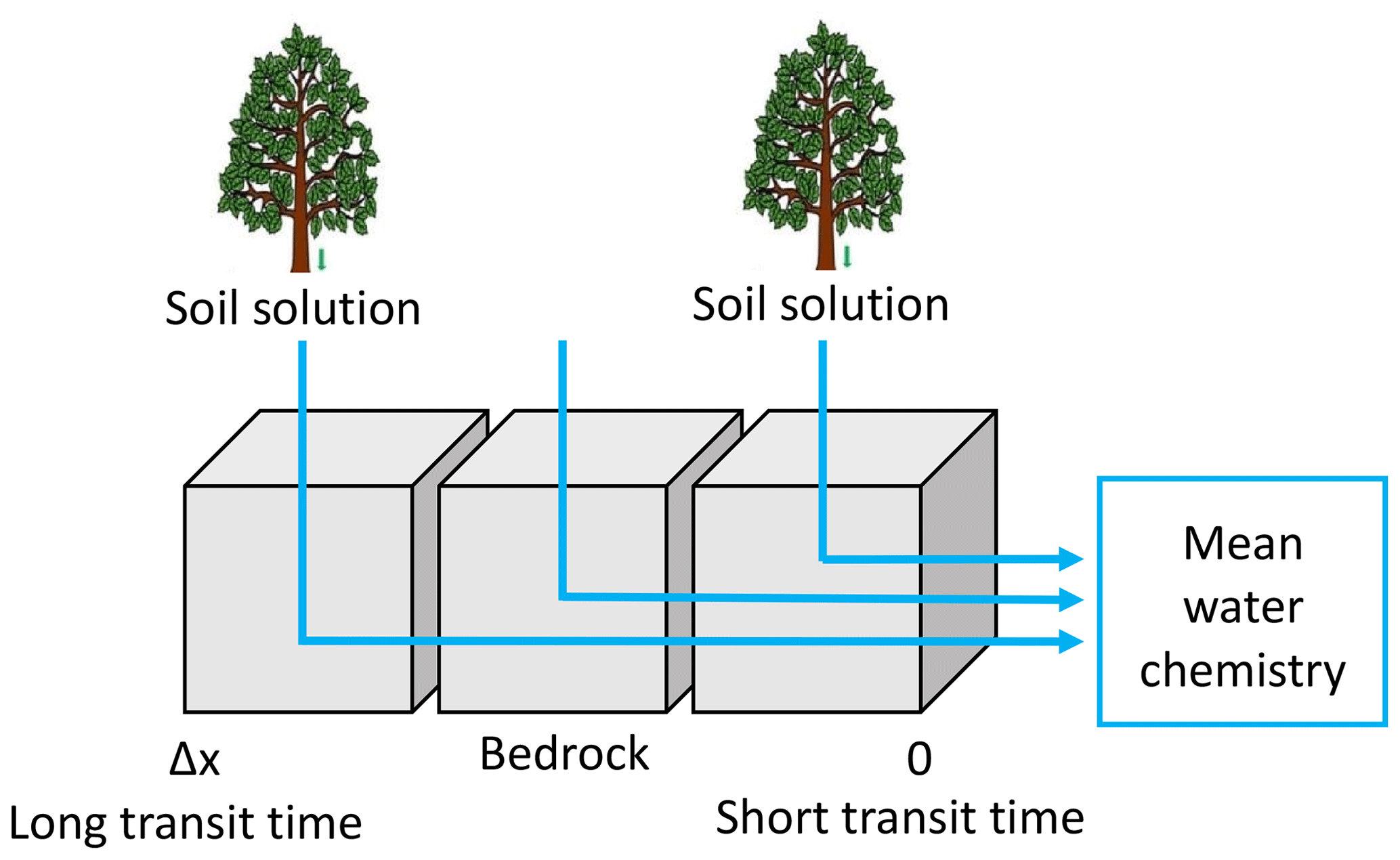
Figure 5Conceptual scheme used in the modeling of the water chemistry. The soil solutions are used as input solution. Cells represent the grid of the reactive-transport code KIRMAT. The regolith is discretized into a 1D succession of cells along the active parts of the flow lines determined by the NIHM hydrological model. The hydrogeochemical model KIRMAT evaluates transport and geochemical processes within each cell. The integrated chemistry of sampled waters is the arithmetic mean of solute concentrations with regularly distributed inlet points along a stream line.
Data related to the regolith properties, such as the mineralogical compositions, the mineral reactive surfaces and the thermodynamic and kinetic constants are given in Ackerer et al. (2018) and in the Supplement (Tables S10 to S14). Mineral phases are assumed to be homogeneously distributed over the regolith layer. By following this strategy, the simulations that consider soil solutions percolating at the upper part of the catchment reflect the chemical evolution of waters with long path lengths and long transit times within the aquifer. By contrast, shorter path lengths and shorter transit times are associated with the percolation of soil solutions that occurs in the vicinity of the sampling locations (Fig. 5). Because the springs or the piezometers collect waters from different origins and with various transit times, integration along each water flow line was performed. The aim of the integration is to determine the mean chemical composition resulting from the mixing of the waters characterized by variable transit times (Fig. 5). The integrated chemical composition of the waters provided by a given flow line is calculated by taking the arithmetic mean of the solute concentrations calculated by the succession of the KIRMAT simulations along the flow line (Fig. 5). This arithmetic mean reflects a simple full mixing of uniform water fluxes along a stream line irrespective of the short or long transit times. In other words, the geochemical simulations are based on the hypothesis of spatially homogenous water–rock interactions along the flow lines. The soil solutions are assumed to percolate uniformly within the aquifer and are then conveyed along the slopes by uniformly distributed masses of water until they reach the sampling locations. When needed, the eventual calculation of water chemistry exiting several stream lines reaching a sampling location accounts for the spreading associated with various flow paths, spatial variability of water velocities and related travel times.
4.1 Spatial variability of the flow lines
The results provided by the hydrological code NIHM show that to the first order, the Strengbach catchment is well drained and that the topography exerts an important control on the flow line distribution (Fig. 4). Along the hillsides presenting linear or slightly convex slopes, the water flow lines show simple characteristics. The flow paths are nearly parallel, and the water velocities are similar along the different flow lines on this type of hillside. The water velocities tend to increase when moving downstream, with slower velocities near the main crests and higher velocities on the steepest parts of the hillsides. The waters collected along this type of hillside are therefore characterized by small variability of transit times. This is the case for the CS1, CS3 and RH3 spring waters located on the southern and northern parts of the catchment (Fig. 4). This is also the case for the piezometers PZ3 and PZ5 in the southern part of the watershed (Fig. 4). For the sites located on linear or slightly convex slopes (CS1, CS3, RH3, PZ3 and PZ5), all the characteristics of the different flow lines that feed each site are therefore comparable for a given site and for a given date.
By contrast, in the vicinity of the valley and in the topographic depressions, the hydrological modeling indicates that the flow line characteristics are more variable. Because flow lines coming from different hillsides can feed a topographic depression, mixing of different flow lines with variable flow paths and contrasted water velocities can occur at these locations. The waters collected in valleys or in topographic depressions are therefore characterized by a higher variability of transit times. This is the case for the CS2 and CS4 springs, which are located in a depression, along the small valley, and surrounded by slopes with various orientations, and a complex flow line distribution (Fig. 4). For these two springs, the characteristics of the different flow lines can be different for a given date.
4.2 Temporal variability of the flow lines
Hydrological modeling under general transient conditions can render the evolution over time of water flows in the watershed but also of other hydraulic variables. As an example, after an important rainfall event (30 March 2010 in Fig. 6), snapshots of the integrated hydraulic conductivity (modeled via the Van Genuchten formulation) in the subsurface and simulated by NIHM at the scale of the mesh size show increasing values with decreasing elevation in the watershed. The same observation holds for conductivities during drought periods (see 29 November 2011, in Fig. 6). Provided that the hydraulic head gradient is largely dominated by the topography and therefore almost constant over time (Fig. 6), the water velocities are increasing along the flow lines from crests to valleys, irrespective of the wet versus dry hydrological periods. However, it is noticeable that wet periods are favorable to a large extension in the valleys of high values of depth-averaged hydraulic conductivity, indicating that the aquifer is locally almost completely saturated from bottom to top (e.g., values of m s−1 in Fig. 6 for a saturated bound at m s−1).
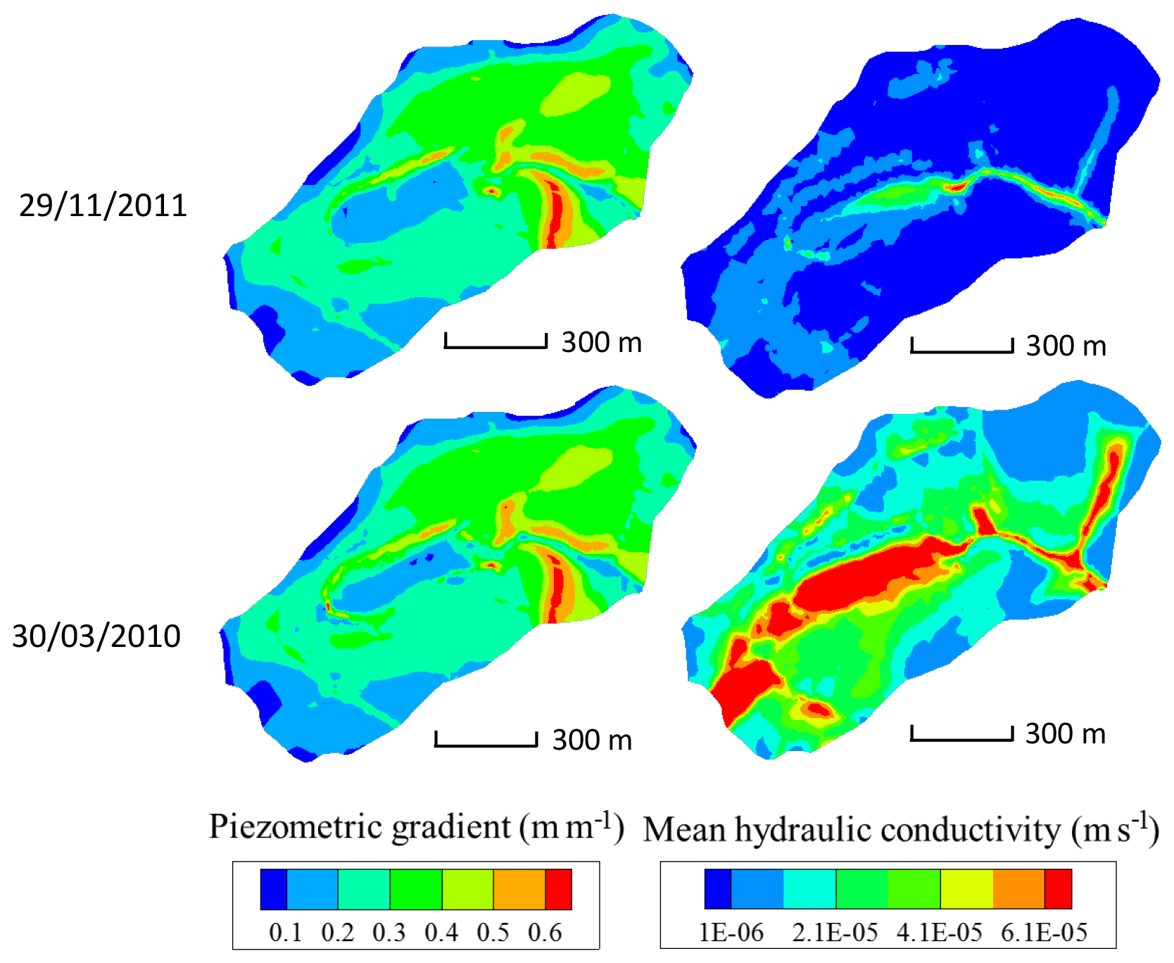
Figure 6Maps of piezometric gradient and depth-integrated hydraulic conductivity for the Strengbach catchment, as simulated by NIHM, on 29 November 2011 (dry period) and 30 March 2010 (high-flow period). The mean hydraulic conductivity is integrated normal to the bedrock of the aquifer and thus depends on the water saturation of the vadose zone and the location of the water table.
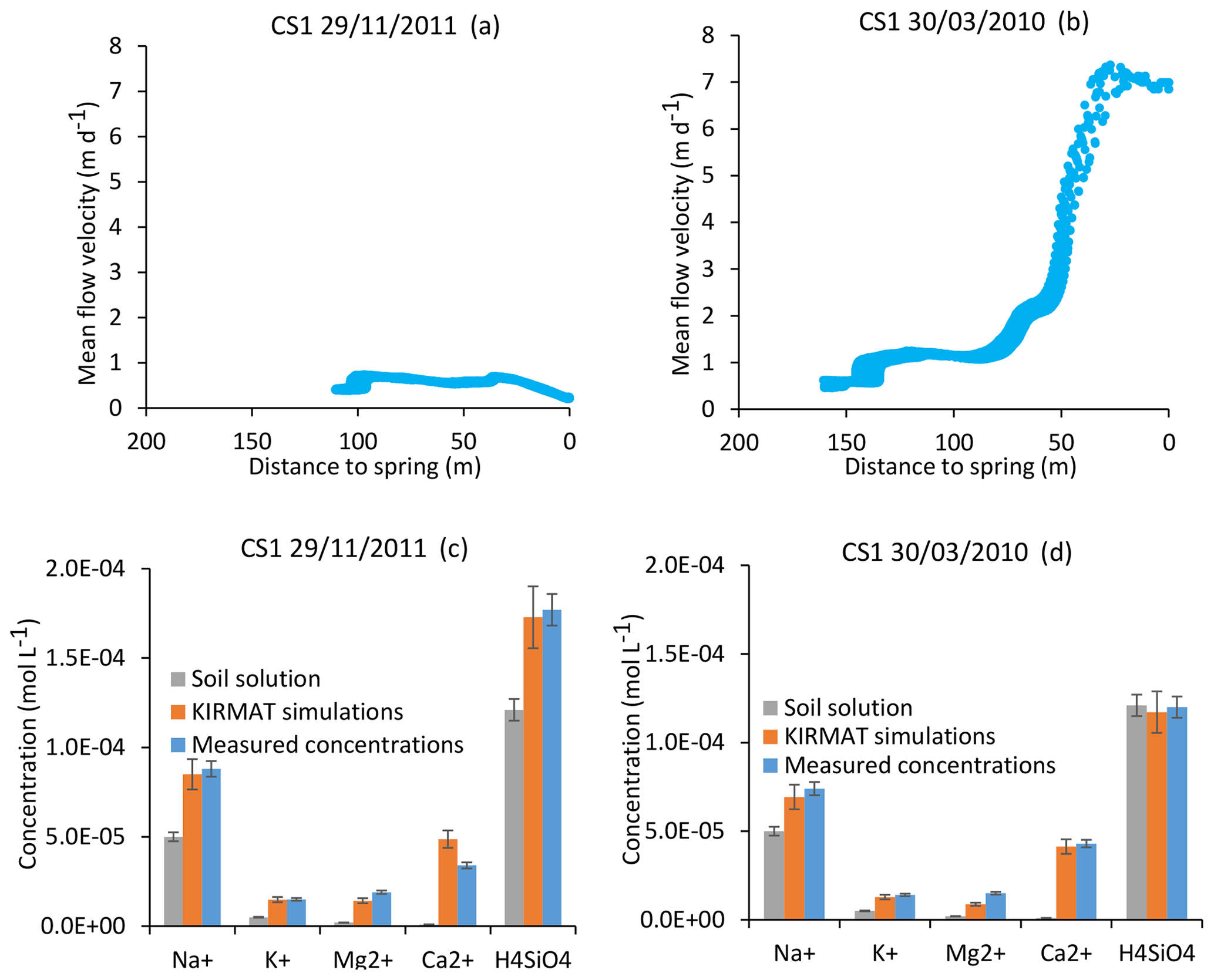
Figure 7Simulation results for the CS1 spring for an important drought (29 November 2011) and a strong flood event (30 March 2010). At the top, active parts of the flow lines bringing the waters to the CS1 spring for the two sampling dates (a, b). Below, simulated chemical compositions of CS1 spring waters after integration along the flow lines and comparison with the initial soil solution and the spring chemistry data (c, d). Error bars show analytical uncertainties on measured concentrations and induced uncertainties in model results (the propagation in the KIRMAT simulations of analytical uncertainties from pH and chemical concentrations measured in the soil solutions).
For the CS1 spring, the mean flow velocities along the flow lines vary from approximately 1 to 7 m d−1 between the severe drought of 29 November 2011 and the strong flood of 30 March 2010 (Fig. 7a and b). These events correspond to the annual minimum and maximum flow rates at the outlet of the Strengbach watershed. For the same dates, the mean velocities vary from 2–12, 1–4 and 1–9 m d−1 for the springs CS2, CS3 and CS4, respectively. The variations from drought to flood are very similar for the piezometer waters, with velocities in the ranges 2–10 and 2–12 m d−1 for the PZ3 and PZ5 piezometers, respectively. The RH3 spring located on a steeper part of the northern slopes exhibits flow velocity variations from 5 to 20 m d−1 from dry to flood conditions.
In addition to the flow velocity variations, the hydrological simulations also reveal variability in the lengths of the active parts of the flow lines. For illustration, the active parts of the flow lines are reduced from 160 to 110 m from the flood to the drought events for the CS1 spring (Fig. 7a and b). Such variability is triggered by the particular seasonal variations of the hydraulic conductivities within the catchment. After a large amount of precipitation, high water content and large integrated hydraulic conductivities (sometimes up to the saturated bound) are simulated in the vicinity of the crests and all along the small valley of the catchment (Fig. 6). During periods of drought, the simulations indicate a strong decrease in hydraulic conductivities close to the main crests and much smaller variations at mid-slopes (Fig. 6). The crests rapidly dry out, whereas the areas at mid-slopes still supply some water to the stream network. These contrasting hydrological behaviors result from the differences in aquifer thickness and water storage between the crests and the other parts of the catchment (Fig. 2). A thin aquifer, flow divergence and the absence of feeding areas prevent large water storage on the crests, in opposition to mid-slope parts with much thicker aquifers and the presence of feeding areas upstream. This particular pattern simulated for the hydraulic conductivities implies that the active parts of the flow lines extend up the main crests during important floods, whereas they are limited to mid-slopes after a long dry period.
The consequence of this hydrological functioning is to moderate the seasonal variations of the transit times of waters, as the active lengths of flow lines vary simultaneously with water flow rates. Calculations indicate that for the spring and piezometer waters collected in this study, the mean transit times of waters only vary from approximately 1.75 to 4 months between the strongest flood and the driest conditions. Notably, these short subsurface water transit times are explained by the small size of the catchment and the steep slopes.
5.1 CS1 and CS3 springs (southern slope)
The CS1 and CS3 springs emerge on the same slope and drain the same rocks. Their hydrological behavior is also very similar in terms of flow lines and water transit times. The interesting consequence of the simple flow line distribution for these springs is that a single flow line can be considered as representative of all the flow lines that are feeding the spring, irrespective of the hydrological conditions. Hydrogeochemical simulations were performed along a single flow line for different hydrological periods using the methodology illustrated in Fig. 5. The case of CS1 spring is used below to highlight the main results obtained from this approach. For the strong flood of 30 March 2010, the KIRMAT simulations modeling the waters coming from the vicinity of the spring and characterized by short transit times produced solutions that were too diluted, whereas the waters coming from the main crests were too concentrated to reproduce the spring water chemical composition. However, after an integration of all the waters arriving at CS1 with the different transit times employed for the simulation, the resulting geochemical composition correctly reproduces the chemical composition of CS1 spring water at this date (H4SiO4, Na+, K+, Mg2+ and Ca2+ concentrations; Fig. 7d). A similar conclusion is obtained for the important drought of 29 November 2011. Again, geochemical integration of all the waters arriving at CS1 along a water line but with different transit times correctly reproduces the chemical composition of the CS1 spring waters collected on this date (Fig. 7c). This comment applies regardless of the time period considered.
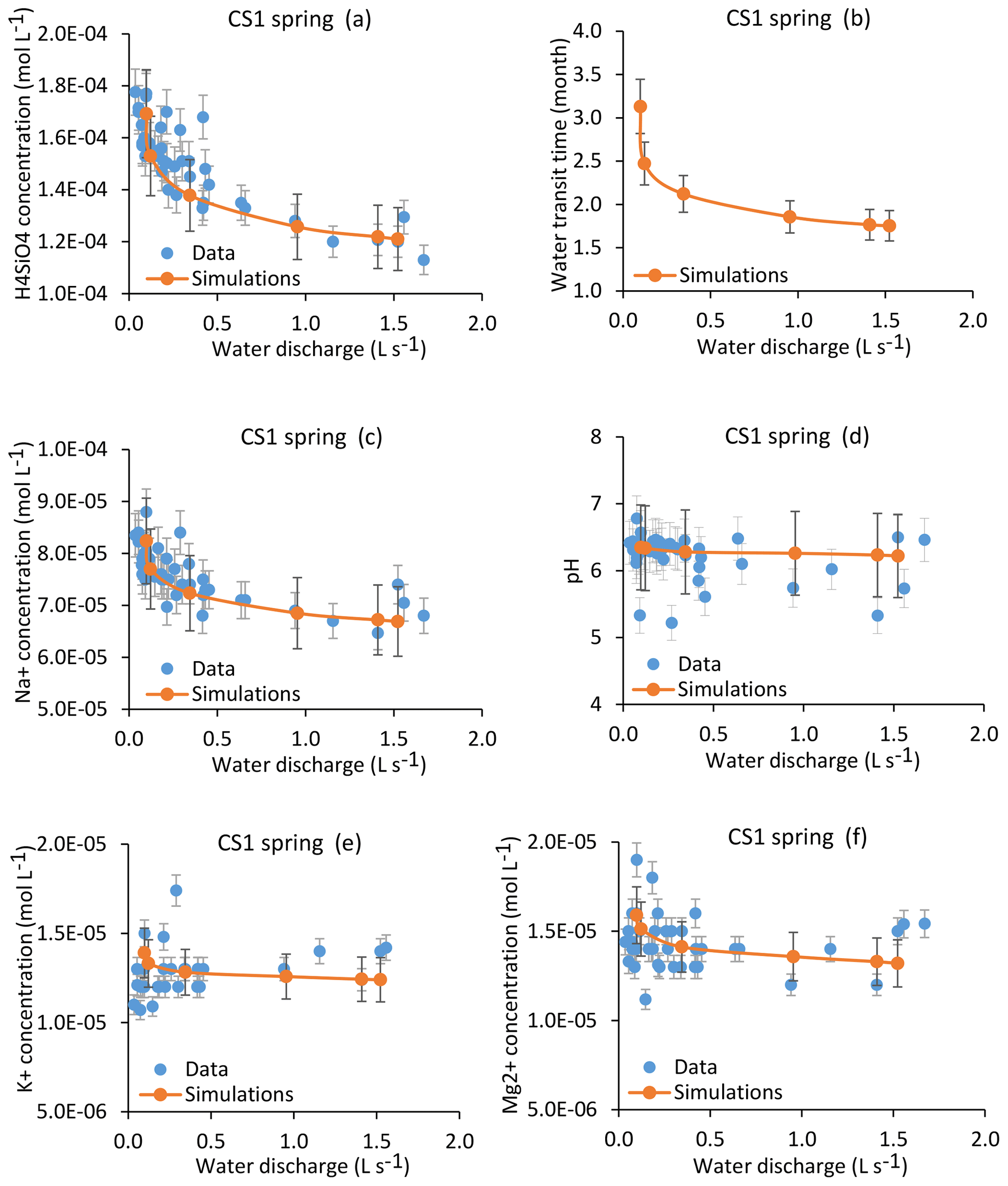
Figure 8Simulation results for the CS1 spring over the whole range of the water discharges from the spring. Results are presented for H4SiO4, Na+, K+ and Mg2+ concentrations (a, c, e, f); pH (d); and mean water transit time (b). Red lines indicate simulated parameters after integration along the flow lines, and blue points show measured values collected between 2005 and 2015. Corresponding dates and data for the modeled samples are given in Table 1. The overall geochemical database is available in Table S1. Error bars show analytical uncertainties on measured concentrations and induced uncertainties in model results (the propagation in the KIRMAT simulations of analytical uncertainties from pH and chemical concentrations measured in the soil solutions). Fitting a power law of type along the C–Q relations gives the following parameters: , ; , ; , ; , .
The coupled hydrological and hydrogeochemical approach has been applied for the CS1 spring for six dates covering the whole range of the water discharges of the spring (Table 1). The modeling results capture the seasonal variations of the water chemical composition of the CS1 spring over the whole range of observed flow rates at CS1 (Fig. 8). Simulations in particular reproduce the 20 %–30 % variation in H4SiO4 concentrations (Fig. 8a), the 10 %–20 % variation in Na+ concentrations (Fig. 8c), and the relatively stability of the K+, Mg2+ and pH of the CS1 waters (Fig. 8e, f and d). The response of each chemical element to a change in water discharge is related to the initial soil solution concentration, the nature of primary minerals controlling its budget and the degree of its incorporation into clay minerals. Specific concentration–mean-transit-time relations (C–MTT relations) explain why the response of solute concentrations to hydrological changes (C–Q relations) is different for each element (Fig. 9). Similar results are obtained for the CS3 spring (Fig. S1), showing, as for the CS1 spring, that the model correctly simulates the water chemical composition of the CS3 spring.
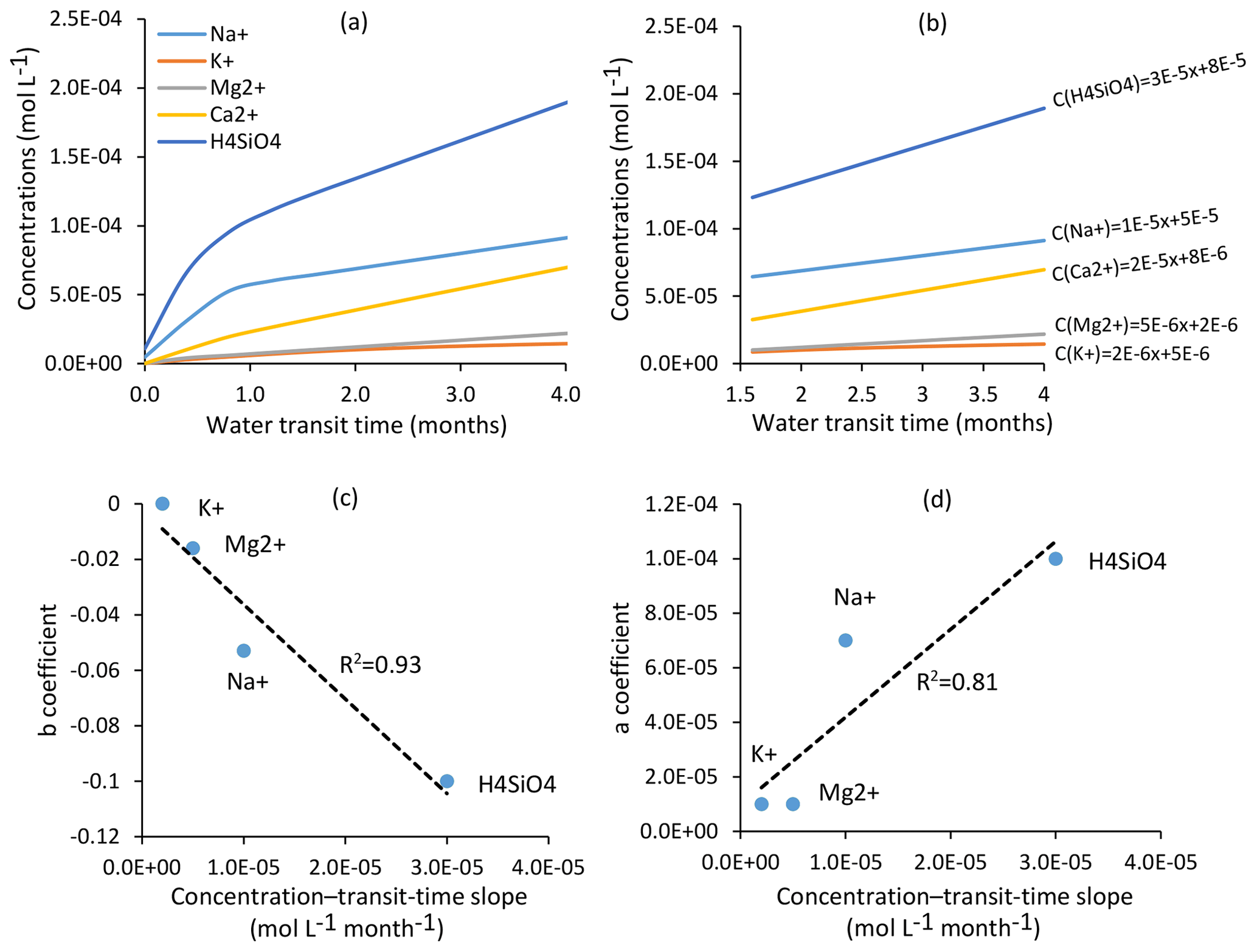
Figure 9(a) Evolution of solute concentrations for H4SiO4, Na+, K+, Mg2+ and Ca2+ as a function of mean water transit time in the Strengbach watershed. Water transit times are between 1.75 and 4 months for all the springs and piezometers in this study. (b) Focus on the transit time window (1.75–4 months) for the studied waters and equations linking mean water transit times and concentrations for H4SiO4, Na+, K+, Mg2+ and Ca2+. Relations between transit times and concentrations are linear within this window; (c) relations between “b” coefficients () and the concentration-transit time slopes for the chemical elements. (d) Relations between “a” coefficients () and the concentration-transit time slopes for the chemical elements. Elements with significant concentration–mean-transit-time slopes are slightly chemodynamic (e.g., H4SiO4 and Na+), while elements with low concentration–mean-transit-time slopes are almost chemostatic in the watershed (e.g., K+ and Mg2+). Ca2+ is not shown in panels (c) and (d) as this element is affected by a strong multi-annual concentration decrease that prevents a meaningful C–Q power-law analysis (Ackerer et al., 2018).
Because the lengths of the flow lines vary over time, the patterns of dissolution rates for primary minerals and precipitated amount of clay minerals are mainly controlled by the spatial and temporal variability of the flow lines. Under wet conditions, the upper parts of the catchment are the areas of maximal dissolution rates of primary minerals and of maximal formation of clay minerals in the regolith. Under dry conditions, the dissolution and precipitation are maximal at mid-slopes, as the upper parts of the catchment are simply dry.
5.2 PZ3 and PZ5 piezometers (southern slope)
The two piezometers PZ3 and PZ5 are located on the southern part of the catchment, and their waters drain a granitic bedrock similar to that drained by the CS sources. As for the CS1 and CS3 springs, the NIHM modeling results show that the flow lines arriving at the PZ3 piezometer are characterized by a relatively simple distribution (Fig. 4). For the PZ5 piezometer located downstream, the flow lines cover a larger area on the slope, especially during droughts (Fig. 4). However, for a given date, all the flow lines show similar velocities, with particularly fast flow in the lower portion of the hillslope. These results imply that, as for the CS1 and CS3 springs, the hydrogeochemical simulations of PZ3 and PZ5 piezometer waters can be performed by relying upon a single flow line representative of all the waters collected by the piezometers on a given date. The geochemical integration is able to reproduce the chemical composition of the waters of the two piezometers, as illustrated in Fig. 10 for the flood of 5 May 2015 and in Fig. S2 for the dry conditions of 10 November 2015. Together, these modeling results show that the flow along linear or slightly convex slopes on the southern part of the catchment allows the water chemistry of each sampling site to be correctly captured with a straightforward integration along a single and representative flow line.
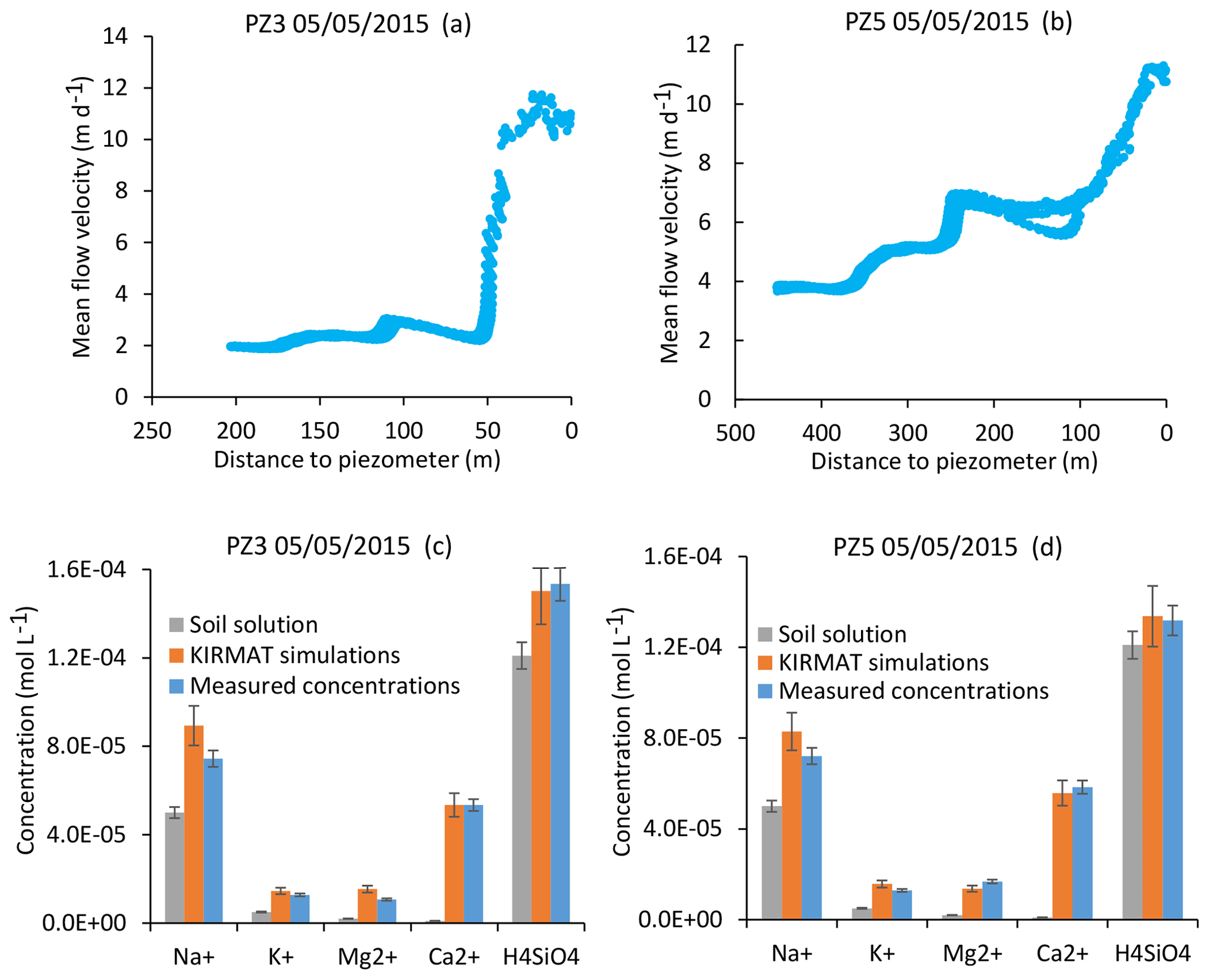
Figure 10Simulation results for the PZ3 and PZ5 piezometers for a flood event (5 May 2015). (a, b) Active parts of the flow lines that bring waters to the two sampling sites. (c, d) Simulated chemical compositions of the piezometer waters after integration along the flow lines and comparison with the initial soil solution and the water chemistry data. Error bars show analytical uncertainties on measured concentrations and induced uncertainties in model results (the propagation in the KIRMAT simulations of analytical uncertainties from pH and chemical concentrations measured in the soil solutions).
5.3 The CS2 and CS4 springs (in the valley axe)
CS2 and CS4 spring waters drain the same granitic bedrock as the CS1 and CS3 waters but are located in the direction of the small valley of the Strengbach stream and surrounded by slopes of various orientations and inclinations (Fig. 4). Consequently, the distribution of the flow lines is much more scattered than for the CS1 and CS3 springs. For the CS2 spring, and for all the hydrological conditions, two different groups of flow lines have been determined by the backtracking approach: a northern group characterized by relatively slow velocities and a southern group with higher velocities (Figs. 4 and 11a, b). This scattered distribution of the flow lines implies that a single specific flow line cannot be representative of all the waters collected by the spring. The flow lines calculated using the NIHM model allow the trajectories of the waters within the watershed to be constrained; however, the simulations performed in this study cannot provide the mass fluxes of water carried by each flow line. Consequently, a straightforward calculation of the chemistry of the CS2 spring, such as depicted above for CS1, is not applicable because the mixing proportions between the different flow lines are unknown.
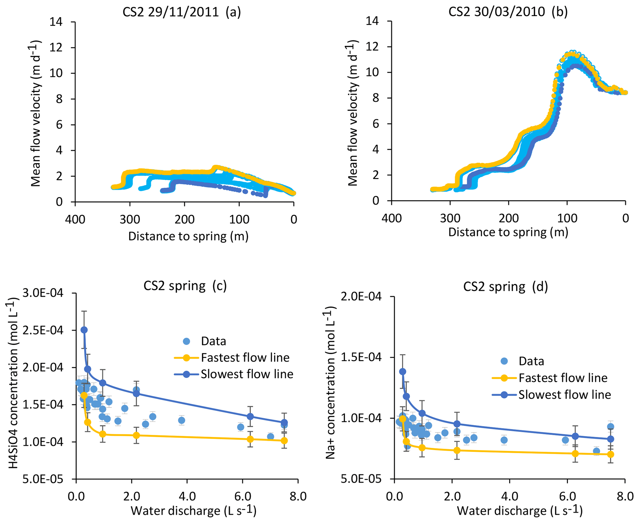
Figure 11Simulation results for the CS2 spring. (a, b) Active parts of the flow lines that bring water to the CS2 spring for drought (29 November 2011) and flood (30 March 2010) events (a, b). The CS2 location results in more scattered flow lines than for the CS1 spring. (c, d) Simulation results for the CS2 spring over the whole range of experienced discharges. Blue lines indicate simulated parameters after integration along the slowest flow line, yellow lines indicate simulated parameters after integration along the fastest flow line, and blue points show measured values collected between 2005 and 2015 (data in Tables 1 and S2). Error bars show analytical uncertainties on measured concentrations and induced uncertainties in model results (the propagation in the KIRMAT simulations of analytical uncertainties from pH and chemical concentrations measured in the soil solutions).
Alternatively, it is possible to determine the concentrations in the waters carried by the slowest and the fastest flow lines that are feeding the spring and to compare the results with the observed chemistry of the spring water. The results indicate that for all the hydrological conditions, the concentrations calculated from the geochemical integration along the slowest and the fastest flow lines are able to correctly frame the chemical composition in terms of H4SiO4, Na+, K+, Mg2+, and Ca2+ of the CS2 spring waters (results are reported for H4SiO4 and Na+ in Fig. 11c and d). The modeling results for CS2 also suggest that the contributions of the slow and fast flow lines are comparable over most of the hydrological conditions, as the observed concentrations are in general at the midpoint between the min (i.e., fast) and max (i.e., slow) boundaries (Fig. 11c and d). It is only for the important droughts that the spring chemistry seems to be mainly controlled by the southern and faster group of flow lines. Further works to precisely estimate the mass fluxes of water carried by each flow line are necessary to model the chemistry of the CS2 spring water with a weighted mixing calculation. The same conclusions apply to the CS4 spring located close to CS2.
5.4 The RH3 spring (northern slope)
The RH3 spring is located on the northern part of the catchment (Fig. 4), where steep slopes imply fast water velocities and subparallel flow lines. However, if the distribution of the flow lines on the RH3 hillside is simple (as for the CS1 and CS3 springs) the precise lithological nature of the bedrock drained by the RH3 waters is more difficult to constrain (Ackerer et al., 2018). Unlike the southern slope, the bedrock of the northern part of the catchment reveals a complex lithology, with gneiss outcropping in the upper part of the slope and granite of variable degree of hydrothermal overprinting in the intermediate and lower parts. These lithological variations can explain the differences in chemical composition between the RH3 spring waters and the waters of the southern part of the catchment: the RH3 spring waters are characterized by systematically higher concentrations of K+ and Mg2+ cations but show similar concentrations for the other major elements (Ackerer et al., 2018; Pierret et al., 2018). The vertical extension of the gneiss and the spatial variability of the hydrothermal overprinting along the northern slopes are not well known, with the consequence that a straightforward modeling of water chemistry as done for CS1 is not possible for RH3.
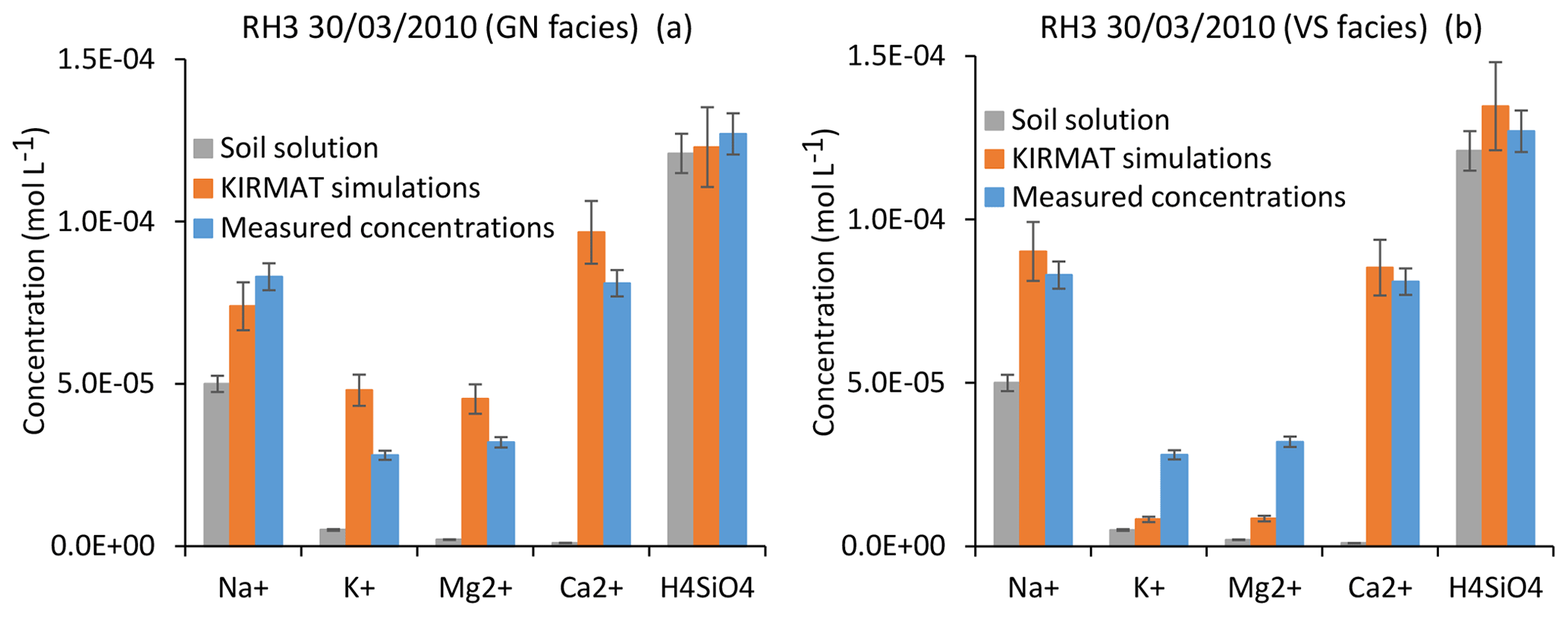
Figure 12Simulation results for the RH3 spring chemistry and for a flood event (30 March 2010). (a) Simulated concentrations by assuming flow lines running through gneiss (GN) only. (b) Simulated concentrations by assuming flow lines running through hydrothermally altered granite (VS) only. Error bars show analytical uncertainties on measured concentrations and induced uncertainties in model results (the propagation in the KIRMAT simulations of analytical uncertainties from pH and chemical concentrations measured in the soil solutions).
Alternatively, simulations of two extreme cases can be performed by assuming that the flow lines only run either on gneiss or on hydrothermally altered granite. When only considering the hydrothermally altered granite (VS facies), the simulated concentrations of H4SiO4 and Na+ are close to the measured ones. Nevertheless, the concentrations of K+ and especially Mg2+ are clearly underestimated (Fig. 12b). In the case of the flow lines only running on gneiss (GN facies), the simulated concentrations of H4SiO4 and Na+ also match the data. However, due to the higher abundance of biotite in the gneiss, the simulated concentrations of K+ and Mg2+ are higher than the measured ones (Fig. 12a). At this stage, it is therefore reasonable to propose that the chemical composition of the RH3 spring waters reflects mixing of the two lithological influences. By assuming a geochemical conservative mixing, which is likely too simplistic a scenario, the results would indicate that the flow line portions running on gneiss and on hydrothermally altered granite count for approximately 40 %–50 % and 50 %–60 % of the total water path length, respectively.
Further works to estimate the location of the contact between gneiss and granite are required for more realistic modeling and hence a deeper interpretation of the chemical composition of the RH3 spring waters. In any case, the important point to stress here based on the above simulations is that the complex lithology and bedrock heterogeneity mainly impact the K+ and the Mg2+ budget of the RH3 waters, but not or only slightly the H4SiO4 and Na+ concentrations, which control the main part of global weathering fluxes carried by the Strengbach spring waters. These results readily explain why, although the RH3 spring waters exhibit higher Mg2+ and K+ concentrations than the other CS springs, they carry relatively similar global weathering fluxes (Viville et al., 2012; Ackerer et al., 2018).
The coupling of the NIHM and KIRMAT codes allows for building a better modeling scheme to those commonly used in previous studies regarding the hydrogeochemical modeling of surface waters at the watershed scale. In such previous works, the geochemical simulations were performed mainly along a single 1D flow line, only characterized by homogeneous mean hydrological properties (Goddéris et al., 2006; Maher, 2011; Moore et al., 2012; Lucas et al., 2017; Ackerer et al., 2018). In a previous study on the Strengbach watershed (Ackerer et al., 2018), the soil solutions were also assumed to percolate in the bedrock only at a single starting point of the flow lines. Although these previous approaches were useful for determining the long-term evolution of regolith profiles and/or the mean chemistry of waters at the multi-annual scale, they cannot be used to discuss the seasonal variations of the water chemical composition. The NIHM–KIRMAT coupling approach makes this possible, as it provides the spatial distribution of the flow lines at the watershed scale and their variations over time. Furthermore, the proposed modeling approach also integrates a soil solution percolation scheme with inlets uniformly distributed along the slope, which is more realistic than a scheme assuming that each sampled site is fed by a single flow line carrying waters with a unique transit time. The good agreement between modeling results and observations over a large panel of hydrological conditions gives strength to the conclusions and implications that can be drawn regarding the hydrogeochemical functioning of this headwater catchment.
6.1 Choices of the reactive surfaces and the kinetic constants
For the geochemical simulations performed in this study, the kinetic constants that were used to describe the dissolution reactions of the primary minerals are standard constants determined through laboratory experiments (Table S12). The reactive surfaces of the primary minerals were calculated by assuming a simple spherical geometry for all the minerals (Table S10). Over the last years, several studies have suggested that the kinetic constants determined through laboratory experiments overestimated the rates of the dissolution reactions in natural environments (White and Brantley, 2003; Zhu, 2005; Moore et al., 2012; Fischer et al., 2014). The origin of this laboratory field discrepancy is still a matter of debate (Fischer et al., 2014). Different processes have been proposed to explain the gap between laboratory and field estimates, such as the crystallographic anisotropy (Pollet-Villard et al., 2016), progressive occlusion of the primary minerals by clays (White and Brantley, 2003), or the formation of passivation layers at the surfaces of the minerals (Wild et al., 2016; Daval et al., 2018). The difficulty to reconcile field and laboratory estimates can also be related to the challenge of defining relevant reactive surfaces at different spatial scales (Li et al., 2006; Navarre-Sitchler and Brantley, 2007).
The present modeling work regarding the Strengbach catchment shows that the chemical composition variability of the spring and piezometer waters is fully captured via geometric reactive surfaces and standard kinetic constants, while respecting the water–rock interaction times within the catchment. This result suggests that the mean rates of the weathering reactions employed in this modeling work are realistic, which in turn implies that the modeling approach developed in this study does not underline significant mismatches between field and laboratory reaction rates. The calculated rates of the dissolution reactions depend on the product between the kinetic constants of the reactions and the mineral reactive surfaces. In the experimental studies performed for determining the kinetic constants of dissolution reactions, the constants are usually determined by normalizing the experimental weathering rates with the Brunauer–Emmett–Teller surfaces determined from experiments of gas absorption (BET surfaces; Chou and Wollast, 1985; Lundström and Öhman, 1990; Acker and Bricker, 1992; Amrhein and Suarez, 1992; Berger et al., 1994; Guidry and Mackenzie, 2003).
Table 3Comparison between BET surfaces and geometric surfaces for the major primary minerals present in a granitic context. BET surfaces were measured via gas absorption experiments in different studies, denoted by superscript letters: a – Berger et al. (1994); b – Chou and Wollast (1985); c – Lundström and Öhman (1990); d – Amrhein and Suarez (1992); e – Acker and Bricker (1992); f – Guidry and Mackenzie (2003). Geometric surfaces were recalculated from the granulometric ranges of the minerals and by assuming a spherical geometry.
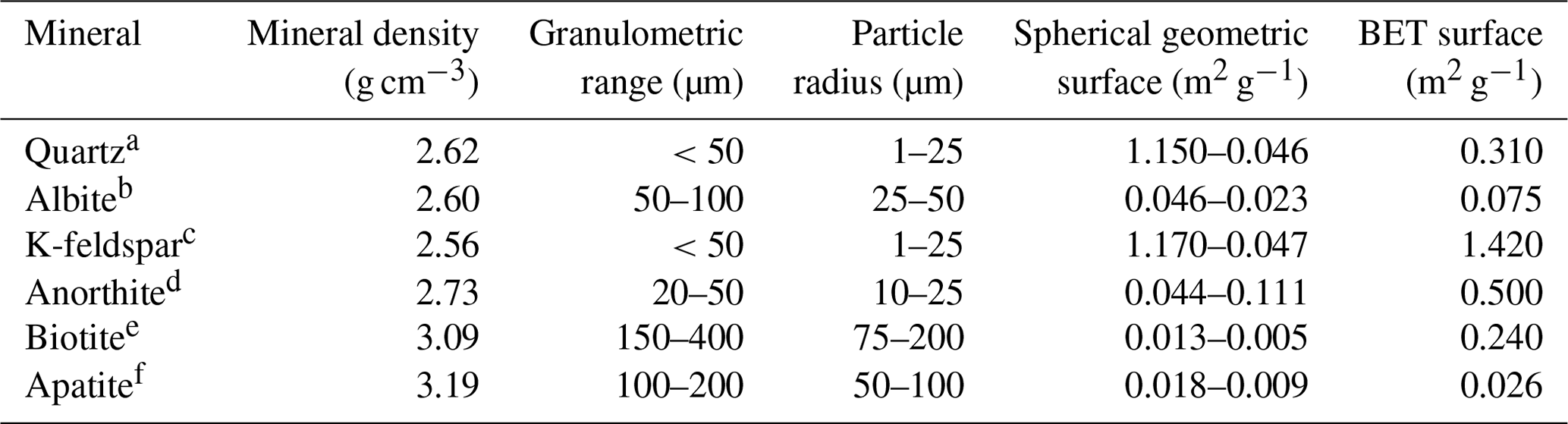
In Table 3, the BET surfaces are compared with the geometric surfaces of the minerals involved in the dissolution experiments, recalculated from the size ranges of the minerals. For most of the minerals (apatite, quartz, albite, K-feldspar and anorthite), the geometric surfaces are within the same order of magnitude as the BET surfaces, even if often slightly lower (Table 3). However, as the BET surfaces are determined with fairly large uncertainties, especially for low BET surfaces (up to ±70 %), and as they can be very different depending on the gas used (up to 50 % of difference between N2 and Kr absorption; Brantley and Mellott, 2000), the above differences between the geometrical and the BET surfaces cannot be considered significant for the majority of minerals used in the Strengbach simulations. A significant difference only appears for biotite, with the geometric surfaces one order of magnitude lower than the BET surfaces (Table 3). However, for biotite, due to its layered structure, it has been shown that approximately 80 %–90 % of the surface area accessible by the gases used to estimate BET surfaces is not accessible for weathering reactions (Nagy et al., 1995).
The above considerations explain why for a granitic bedrock as found in the Strengbach catchment, the geometric surfaces are relevant to describe the surfaces of water–rock interactions at the spatial and temporal scales of this study. An immediate corollary is that the values of the standard kinetic constants (Table S12) are also appropriate to calculate reaction rates with mineral geometric surfaces in our modeling approach. This ability may be related to the fact that all the minerals that have been used in the dissolution experiments and in the kinetic studies were collected in the field (e.g., Acker and Bricker, 1992; Amrhein and Suarez, 1992). These minerals were likely affected by anisotropy, passivation layers and any types of aging effects related to long-term water–rock interactions. Our results might therefore mean that the standard kinetic constants obtained in such experiments integrate the aging effects that have affected the reactivity of the primary minerals in natural environments. This would explain why it is possible to capture the full variability of the water chemistry in a headwater catchment with simple geometric reactive surfaces and standard kinetic constants.
At this stage, the results of our simulations strengthen the idea that the low surfaces calculated from the geometrical shapes of minerals provide good estimates of the reactive surfaces within this type of environment (Brantley and Mellott, 2000; Gautier et al., 2001; White and Brantley, 2003; Zhu, 2005; Li et al., 2017b). They are certainly the values to be used for hydrogeochemical modeling such as that performed in this work, in addition to the use of the experimental kinetic constants for mineral dissolution. These conclusions are certainly not specific to the Strengbach catchment and could be applicable to many other headwater granitic catchments.
6.2 Implications for the acquisition of the water chemistry
The results of the NIHM–KIRMAT hydrogeochemical modeling have strong implications regarding the hydrogeochemical dynamics of the Strengbach watershed. This work reinforces several hypotheses formulated by previous studies conducted in the Strengbach watershed (Viville et al., 2012; Pierret et al., 2014; Pan et al., 2015; Chabaux et al., 2017; Weill et al., 2017; Ackerer et al., 2018) but also provides new insights into the hydrogeochemical functioning of the catchment. Firstly, the modeling results emphasize the importance of water transit times within the watershed as a main feature controlling the chemical composition of subsurface waters. Along all the slopes, the waters coming from the vicinity of the crests and characterized by long transit times systematically render higher concentrations than the waters with shorter pathways and transit times. When the hydrological conditions change from wet to dry periods, the solute concentrations also tend to increase with the increase in the mean transit time of waters. Our results show that for the spring and piezometer waters, the spatial and temporal variations of their geochemical composition are fully explained by the differences in water transit times (Fig. 13). Transit time variations between high and low discharge periods explain the temporal variations of geochemical signatures within each site. Various mean transit times of waters supplying the different sites explain the various chemical compositions between the sites (Fig. 13). This key role of the water–rock interaction time is in agreement with previous reactive-transport studies conducted in the Strengbach watershed (Ackerer et al., 2018) and in other sites (e.g., Maher, 2010; Moore et al., 2012; Lebedeva and Brantley, 2013).
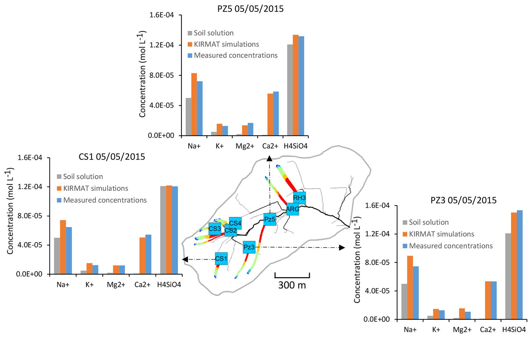
Figure 13Overview of the simulated flow lines in the subsurface that feed with water the geochemical sampling sites CS1, PZ3 and PZ5 on 5 May 2015. The simulated chemical compositions after geochemical integration along the flow lines are compared with the initial soil solution and the spring chemistry data.
This study also provides new constraints on the spatial distribution of the weathering processes. For the modeling strategy employed, the chemical composition of the spring and piezometer waters are calculated by integrating the chemical composition of waters introduced at different starting locations along the active part of the flow lines (Fig. 5). The modeling results show that through the geochemical integration, the concentrated waters coming from the main crests are naturally counterbalanced by the diluted waters infiltrating close to the sampling sites. The solute chemistry is acquired through reactions and weathering processes that are spatially relatively homogenous along the flow lines of the watersheds. This spatial homogeneity of the weathering processes helps us to understand why the chemical fluxes carried by the Strengbach stream (Viville et al., 2012), the chemical fluxes from the Strengbach spring waters (Ackerer et al., 2018) and the weathering fluxes locally determined along a regolith profile sampled in the catchment (Ackerer et al., 2016) are all very similar.
The modeling also shows that the hydrogeochemical functioning of the watershed is properly simulated by water circulations in the shallow subsurface, i.e., in a saprolitic aquifer. No contribution of waters circulating in the deep fracture network of the granitic bedrock and observed during the drilling campaigns (see Chabaux et al., 2017) is necessary. The deep-water circulations are probably disconnected from the shallow subsurface network, as recently suggested by geochemical studies conducted in the Strengbach watershed (Chabaux et al., 2017; Pierret et al., 2018). This is also in agreement with recent hydrological modeling studies arguing that the catchment behaves like a vertically thin but horizontally wide reservoir (Pan et al., 2015; Weill et al., 2017). The modeling results also show that water in the shallow aquifer flows along streamlines with fairly simple geometries. At the scale of the catchment (Fig. 4), the geometry of the flow lines validates the hypothesis based on the geochemical and Sr-U isotopic data that the spring waters of these mid-mountain basins are supplied by waters from distinct flow paths without real interconnections (i.e., the Strengbach and Ringelbach watersheds; Schaffhauser et al., 2014; Pierret et al., 2014). Flow paths are therefore distinct along the slopes and occur within the shallow saprolitic aquifer but are not controlled by deep fractures in the bedrock.
6.3 Origins of general chemostatic behavior and of specific C–Q relations
The hydrogeochemical monitoring of the spring, piezometer and stream waters performed in the Strengbach catchment clearly shows that this catchment has a general chemostatic behavior (e.g., Viville et al., 2012; Ackerer et al., 2018). All the spring and the piezometer waters have chemical concentrations impacted by changes in the hydrological conditions, but the concentration variation ranges are far narrower than variation ranges of water discharges, which define the chemostatic behavior of a hydrological system. For waters showing the largest concentration variations (spring CS1), there is a modest increase of approximately 10 %–30 % in the concentrations of H4SiO4 and Na+ from floods to drought events, while the water discharges may vary by a factor of 15 (Fig. 8). This modest variability of the solute concentrations over a wide range of water discharges is not specific to the Strengbach catchment; it has been observed in several watersheds spanning different climates and hydrological contexts (Godsey et al., 2009; Clow and Mast, 2010; Kim et al., 2017).
Different origins for the chemostatic behavior have been proposed, such as a modification of the mineral reactive surfaces during changing hydrological conditions (Clow and Mast, 2010), a small concentration difference between slow and fast moving waters (Kim et al., 2017), or the fact of reaching an equilibrium concentration along the water pathway (Maher, 2010). The coupled approach NIHM–KIRMAT renews the opportunity to discuss the origin of the chemostatic behavior in catchments. It is worth noting that the acquisition and the evolution of the water chemistry can be simulated along flow lines that have been determined via temporally and spatially distributed hydrological modeling. The strength of this approach is in constraining water transit times independently and before any geochemical simulation.
The results from the hydrological model show that the characteristics of the flow lines are affected by the changes in the hydrological conditions (Sect. 4.2). This hydrological functioning implies a covariation between flow velocity and flow length under changing hydrological conditions, with faster flows along longer paths under wet conditions and slower flows along shorter paths during dry periods. This hydrological behavior attenuates the variations of the water transit times under changing hydrological conditions. It also explains why the mean transit times span much narrower variation ranges than the water discharges at the collected springs. For example, the calculated mean transit times of waters for the CS1 spring vary from 1.75 to 3.13 months between the strongest flood and the driest period that have been studied, whereas the water discharges vary from 1.523 to 0.098 L s−1 (Fig. 8b). Because the time of the water–rock interactions exerts a first-order control on the chemical composition of waters, the weak variability of the mean transit times is directly responsible for the relative stability of the chemical composition of waters within the catchment. A seasonal expansion and contraction of the hydrological network was also recently highlighted in Alpine headwater catchments (Van Meerveld et al., 2019).
In addition to this general chemostatic behavior, each chemical element has a specific response to a change in water transit time, as exemplified in Fig. 9, in which the concentration–mean-transit-time relations (C–MTT relations) for H4SiO4 and the major cations are given. In the relevant transit time window for the spring and piezometer waters (Fig. 9b), the C–MTT relations are linear and C–MTT slopes are significant for H4SiO4, modest for Na+ and weak for Mg2+ and K+ concentrations. The modeling results indicate that the C–MTT slopes are controlled by the competition between primary mineral dissolution and element incorporation into clay minerals. When elemental fluxes from primary mineral dissolution to solution are much higher than fluxes from solution to clay minerals (e.g., H4SiO4), the element can accumulate in solution, resulting in a significant C–MTT slope. By contrast, when elemental fluxes from primary mineral dissolution to solution are only slightly higher than fluxes from solution to clay minerals (e.g., K+), the element accumulates only slowly in solution, resulting in a weak C–MTT slope. Interestingly, when fitting power laws along C–Q relations (C=aQb, in caption of Fig. 8), both “a” coefficient controlling the height of the C–Q laws and “b” coefficient controlling the curvature of the C–Q laws are sensitive to the C–MTT slopes (Fig. 9c and d). The“a” coefficient is positively correlated with C–MTT slopes while the “b” coefficient is negatively correlated. Solute species with significant C–MTT slopes are more chemodynamic and display higher mean annual concentrations (H4SiO4, , ), whereas species with weak C–MTT slopes show low mean annual concentrations and are nearly perfectly chemostatic (, , , ; Figs. 8, 9c and d). Our results show that a better knowledge of C–MTT relations is important to explain the contrasted C–Q shapes of chemical elements.
It is important to underline that the hydrological modeling with the NIHM code is performed independently and before any geochemical simulations with the KIRMAT code. The fact that the flow rates are well reproduced for all the hydrological contexts between 2010 and 2015 supports that the water transit times inferred from the NIHM code are realistic. The fact that the chemical composition of waters is well captured indicates that the combination of the geochemical parameters used in KIRMAT code is able to generate realistic reaction rates, as chemistry is well reproduced while respecting realistic water transit times. No modifications of the reactive surfaces and of the dissolution kinetic constants were necessary to reproduce the seasonal variability of the water chemistry. It is also important to emphasize that the simulated chemical compositions of waters remain far from a state of chemical equilibrium with respect to primary minerals. The calculated Gibbs free energy for the primary minerals ranges from −120 to −100 kJ mol−1 for apatite, −90 to −80 kJ mol−1 for biotite and anorthite, and −30 to −20 kJ mol−1 for albite and K-feldspar. These far-from-equilibrium values for the Gibbs free energy imply that the reaction rates calculated using hydrogeochemical codes such as KIRMAT, which are based on the transient state theory (TST, Eyring, 1935; Murphy and Helgeson, 1987), are realistic for most of the primary minerals in this type of hydrological context. Regarding the simulations performed in this study, the relatively short residence times of waters and the precipitation of clay minerals prevent a state of chemical equilibrium being reached between waters and primary minerals at the watershed scale. A water transit time around 8–12 years and a distance as long as 15–20 km would be necessary to reach a chemical equilibrium between water and primary minerals (see Ackerer et al., 2018). This long equilibrium length is explained by the precipitation and the dynamic behavior of clay minerals removing ions from solution and retarding chemical equilibrium with respect to primary minerals. Relying upon a clay solid solution is also appropriate to mimic the clay mineral dynamics in this type of watershed, and a clay mineral assemblage precipitating at thermodynamic equilibrium is able to generate reliable water chemistry (this study) and a realistic amount of clay minerals (mass fraction of clay minerals of 2 %–3 % in the regolith after 20 kyr of weathering; more detail can be found in Ackerer et al., 2018).
Our results indicate that it is not necessary to mix in different proportions of soil and deep waters to generate chemostatic behavior, as proposed by Zhi et al. (2019). Chemostatic behavior can be generated within a single regolith layer with a homogeneous mineralogy, if as demonstrated, the transit time variability of shallow subsurface waters is dampened by seasonal fluctuations of flow line properties. A large storage of primary minerals and weathering product in the subsurface, as proposed in Musolff et al. (2015), is required but not sufficient to generate chemostatic behavior. Chemostatic behavior also depends on the covariation between flow velocities and flow lengths under changing hydrological conditions. Chemostatic behavior is not explained by a modification of the reactive surface of minerals in the subsurface (i.e., Clow and Mast, 2010), or by an absence of chemical contrast between slow and rapid flows (i.e., Kim et al., 2017). The precipitation of clay minerals is essential to correctly capture the water chemistry in our study, but the dissolution or redissolution of clays is not a key process to explain chemostatic behavior (i.e., Li et al., 2017a). Our study clearly supports the idea defended by Herndon et al. (2018) that a spatial and temporal variability in flow paths is a key process to explain C–Q relations in this type of headwater catchment. Our conclusions can most likely be extended to the other mountainous and relatively steep watersheds of this type, in which water pathways and short transit times are mainly controlled by gravity-driven flow along slopes (Weill et al., 2019).
This study exemplifies the potential of coupling of low-dimensional and depth-integrated hydrological modeling with hydrogeochemical modeling as a way to better understand variability over time and space of the composition of surface and subsurface waters. The independent estimation of the water transit times provided by hydrological simulations is a clear added value to constrain the geochemical modeling approaches. Our study demonstrates that the seasonal variability of hydraulic conductivities along the slopes is a key process to understand the dynamics of flow lines and the changes of water transit times in the watershed. The variations in flow line distributions from drought to flood events result in a modest seasonal variability of mean water transit times, which in turn explains the relative stability of the solute concentrations in waters. Our results also show that a better knowledge of the concentration–mean-transit-time relations (C–MTT relations) is an interesting new step to understand the diversity of C–Q shapes for different chemical elements. The consistency between measured and modeled concentrations while respecting the water–rock interaction times provided by the hydrological simulations shows that it is possible to capture the chemical composition of waters with simply determined reactive surfaces and standard kinetic constants. The results of our simulations strengthen the idea that the low surfaces calculated from the geometrical shapes of minerals are a good estimate of the reactive surfaces in this type of granitic catchment, and certainly the values to be used for hydrogeochemical modeling such as that performed in this work, in addition to the use of the experimental kinetic constants for mineral dissolution.
Data are available in the Supplement and in the publications from the LHyGeS laboratory and OHGE observatory (“Observatoire Hydrogéochimique de l’Environnement”, OHGE; http://ohge.unistra.fr; El Gh'Mari, 1995; Fichter et al., 1998; Viville et al., 2012; Gangloff et al., 2014, 2016; Prunier et al., 2015; Pan et al., 2015; Ackerer et al., 2016, 2018; Beaulieu et al., 2016; Chabaux et al., 2017, 2019; Schmitt et al., 2017, 2018; Daval et al., 2018; Pierret et al., 2018).
The supplement related to this article is available online at: https://doi.org/10.5194/hess-24-3111-2020-supplement.
JA was involved in the KIRMAT modeling, the coupling between NIHM and KIRMAT, data interpretation, and the manuscript redaction. BJ, FD and SW were involved in the NIHM model development. YL and BF were involved in the KIRMAT model development. DV was involved in the acquisition of spring chemical data. FC was involved in the manuscript redaction and in the data interpretation.
The authors declare that they have no conflict of interest.
This work benefited from fruitful discussions with Philippe Ackerer and Damien Daval. The authors thank all the reviewers for their constructive comments that improved the quality of the paper.
This research has been supported by the French ANR Program (project CANTARE-Alsace (grant no. ANR-15-CE06-0014)).
This paper was edited by Jan Seibert and reviewed by Laurent Pfister, Camille Bouchez, and three anonymous referees.
Acker, J. G. and Bricker, O. P.: The influence of pH on biotite dissolution and alteration kinetics at low temperature, Geochim. Cosmochim. Ac., 56, 3073–3092, 1992.
Ackerer, J., Chabaux, F., Van der Woerd, J., Viville, D., Pelt, E., Kali, E., Lerouge, C., Ackerer, P., Di Chiara Roupert, R., and Négrel, P.: Regolith evolution on the millennial timescale from combined U–Th–Ra isotopes and in situ cosmogenic 10Be analysis in a weathering profile (Strengbach catchment, France), Earth Planet. Sc. Lett., 453, 33–43, 2016.
Ackerer, J., Chabaux, F., Lucas, Y., Clément, A., Fritz, B., Beaulieu, E Viville D., Pierret, M.C., Gangloff, S., and Négrel, P.: Monitoring and reactive-transport modeling of the spatial and temporal variations of the Strengbach spring hydrochemistry, Geochim. Cosmochim. Ac., 225, 17–35, 2018.
Ameli, A. A., Beven, K., Erlandsson, M., Creed, I. F., McDonnell, J. J., and Bishop, K.: Primary weathering rates, water transit times, and concentration-discharge relations: A theoretical analysis for the critical zone, Water Resour. Res., 53, 942–960, 2017.
Amrhein, C. and Suarez, D. L.: Some factors affecting the dissolution kinetics of anorthite at 25 C, Geochim. Cosmochim. Ac., 56, 1815–1826, 1992.
Bao, C., Li, L., Shi, Y., and Duffy, C.: Understanding watershed hydrogeochemistry: 1. Development of RT-Flux-PIHM, Water Resour. Res., 53, 2328–2345, 2017.
Beaulieu, E., Goddéris, Y., Donnadieu, Y., Labat, D., and Roelandt, C.: High sensitivity of the continental-weathering carbon dioxide sink to future climate change, Nat. Clim. Change, 2, 346–349, 2012.
Beaulieu, E., Lucas, Y., Viville, D., Chabaux, F., Ackerer, P., Goddéris, Y., and Pierret, M. C.: Hydrological and vegetation response to climate change in a forested mountainous catchment, Modeling Earth Systems and Environment, 2, 1–15, 2016.
Beisman, J. J., Maxwell, R. M., Navarre-Sitchler, A. K., Steefel, C. I., and Molins, S.: ParCrunchFlow: an efficient, parallel reactive transport simulation tool for physically and chemically heterogeneous saturated subsurface environments, Computat. Geosci., 19, 403–422, 2015.
Berger, G., Cadore, E., Schott, J., and Dove, P. M.: Dissolution rate of quartz in lead and sodium electrolyte solutions between 25 and 300 C: Effect of the nature of surface complexes and reaction affinity, Geochim. Cosmochim. Ac., 58, 541–551, 1994.
Brantley, S. L. and Mellott, N. P.: Surface area and porosity of primary silicate minerals, Am. Mineral., 85, 1767–1783, 2000.
Camporese, M., Paniconi, C., Putti, M., and Orlandini, S.: Surface-subsurface flow modeling with path-based runoff routing, boundary condition-based coupling, and assimilation of multisource observation data, Water Resour. Res., 46, W02512, https://doi.org/10.1029/2008WR007536, 2010.
Chabaux, F., Viville, D., Lucas, Y., Ackerer, J., Ranchoux, C., Bosia, C, Pierret, M.C., Labasque, T., Aquilina, L., Wyns, R., Lerouge, C., Dezaye, C., and Négrel, P.: Geochemical tracing and modeling of surface and deep water–rock interactions in first-order granitic watersheds (Strengbach and Ringelbach CZOs, France), Acta Geochim., 36, 363–366, 2017.
Chabaux, F., Stille, P., Prunier, J., Gangloff, S., Lemarchand, D., Morvan, G., Négrel, J., Pelt, E., Pierret, M. C., Rihs, S., Schmitt, A. D., Trémolières, T., and Viville, D.: Plant-soil-water interactions: Implications from U-Th-Ra isotope analysis in soils, soil solutions and vegetation (Strengbach CZO, France), Geochim. Cosmochim. Ac., 259, 188–210, 2019.
Chorover, J., Derry, L. A., and McDowell, W. H.: Concentration-Discharge Relations in the Critical Zone: Implications for Resolving Critical Zone Structure, Function, and Evolution, Water Resour. Res., 53, 8654–8659, 2017.
Chou, L. and Wollast, R.: Steady-state kinetics and dissolution mechanisms of albite, Am. J. Sci., 285, 963–993, 1985.
Clow, D. W. and Mast, M. A.: Mechanisms for chemostatic behavior in catchments: implications for CO2 consumption by mineral weathering, Chem. Geol., 269, 40–51, 2010.
Daval, D., Calvaruso, C., Guyot, F., and Turpault, M. P.: Time-dependent feldspar dissolution rates resulting from surface passivation: Experimental evidence and geochemical implications, Earth Planet. Sc. Lett., 498, 226–236, 2018.
Diamond, J. S. and Cohen, M. J.: Complex patterns of catchment solute–discharge relationships for coastal plain rivers, Hydrol. Process., 32, 388–401, 2018.
Ebel, B. A. and Loague, K.: Physics-based hydrologic-response simulation: Seeing through the fog of equifinality, Hydrol. Process., 20, 2887–2900, 2006.
El Gh'Mari, A.: Etude minéralogique, pétrophysique et géochimique de dynamique d'altération d'un granite soumis aux dépôts atmosphériques acides (bassin versant du Strengbach, Vosges, France). Mécanismes, bilans et modélisation, PhD Thesis, Université Louis Pasteur, Strasbourg, France, 200 pp., 1995.
Eyring, H.: The activated complex in chemical reactions, J. Chem. Phys., 3, 107–115, 1935.
Fichter, J., Turpault, M. P., Dambrine, E., and Ranger, J.: Mineral evolution of acid forest soils in the Strengbach catchment (Vosges mountains, NE France), Geoderma, 82, 315–340, 1998.
Fischer, C., Kurganskaya, I., Schäfer, T., and Lüttge, A.: Variability of crystal surface reactivity: What do we know?, Appl. Geochem., 43, 132–157, 2014.
Gangloff, S., Stille, P., Pierret, M. C., Weber, T., and Chabaux, F.: Characterization and evolution of dissolved organic matter in acidic forest soil and its impact on the mobility of major and trace elements (case of the Strengbach watershed), Geochim. Cosmochim. Ac., 130, 21–41, 2014.
Gangloff, S., Stille, P., Schmitt, A. D., and Chabaux F.: Factors controlling the chemical composition of colloidal and dissolved fractions in soil solutions and the mobility of trace elements in soils, Geochim. Cosmochim. Ac., 189 37–57, 2016.
Gautier, J. M., Oelkers, E. H., and Schott, J.: Are quartz dissolution rates proportional to BET surface areas?, Geochim. Cosmochim. Ac., 65, 1059–1070, 2001.
Gérard, F., Clément, A., and Fritz, B.: Numerical validation of a Eulerian hydrochemical code using a 1D multisolute mass transport system involving heterogeneous kinetically controlled reactions, J. Cont. Hydrol., 30, 201–216, 1998.
Gislason, S. R., Oelkers, E. H., Eiriksdottir, E. S., Kardjilov, M. I., Gisladottir, G., Sigfusson, B., Snorrason, A., Elefsen, S., Hardardottir, J., Torssander, P., and Oskarsson, N.: Direct evidence of the feedback between climate and weathering, Earth Planet. Sc. Lett., 277, 213–222, 2009.
Goddéris, Y., François, L. M., Probst, A., Schott, J., Moncoulon, D., Labat, D., and Viville, D.: Modelling weathering processes at the catchment scale: the WITCH numerical model, Geochim. Cosmochim. Ac., 70, 1128–1147, 2006.
Goddéris, Y., Brantley, S. L., François, L. M., Schott, J., Pollard, D., Déqué, M., and Dury, M.: Rates of consumption of atmospheric CO2 through the weathering of loess during the next 100 yr of climate change, Biogeosciences, 10, 135–148, https://doi.org/10.5194/bg-10-135-2013, 2013.
Godsey, S. E., Kirchner, J. W., and Clow, D. W.: Concentration–discharge relationships reflect chemostatic characteristics of US catchments, Hydrol. Process., 23, 1844–1864, 2009.
Guidry, M. W. and Mackenzie, F. T.: Experimental study of igneous and sedimentary apatite dissolution: control of pH, distance from equilibrium, and temperature on dissolution rates, Geochim. Cosmochim. Ac., 67, 2949–2963, 2003.
Gunduz, O. and Aral, M. M.: River networks and groundwater flow: a simultaneous solution of a coupled system, J. Hydrol., 301, 216–234, 2005.
Gupta, H. V., Kling, H., Yilmaz, K. K., and Martinez, G. F.: Decomposition of the mean squared error and NSE performance criteria: Implications for improving hydrological modelling, J. Hydrol., 377, 80–91, 2009.
Hazenberg, P., Broxton, P., Gochis, D., Niu, G. Y., Pangle, L. A., Pelletier, J. D., Troch, P. A., and Zeng, X.: Testing the hybrid-3-D hillslope hydrological model in a controlled environment, Water Resour. Res., 52, 1089–1107, 2016.
Herndon, E. M., Steinhoefel, G., Dere, A. L., and Sullivan, P. L.: Perennial flow through convergent hillslopes explains chemodynamic solute behavior in a shale headwater catchment, Chem. Geol., 493, 413–425, 2018.
Jeannot, B., Weill, S., Eschbach, D., Schmitt, L., and Delay, F.: A low-dimensional integrated subsurface hydrological model coupled with 2-D overland flow: Application to a restored fluvial hydrosystem (Upper Rhine River–France), J. Hydrol., 563, 495–509, 2018.
Kampf, S. K. and Burges, S. J.: A framework for classifying and comparing distributed hillslope and catchment hydrologic models, Water Resour. Res., 43, W05423, https://doi.org/10.1029/2006WR005370, 2007.
Kim, H., Dietrich, W. E., Thurnhoffer, B. M., Bishop, J. K., and Fung, I. Y.: Controls on solute concentration-discharge relationships revealed by simultaneous hydrochemistry observations of hillslope runoff and stream flow: The importance of critical zone structure, Water Resour. Res., 53, 1424–1443, 2017.
Kirchner, J. W.: Getting the right answers for the right reasons: Linking measurements, analyses, and models to advance the science of hydrology, Water Resour. Res., 42, W03S04, https://doi.org/10.1029/2005WR004362, 2006.
Lebedeva, M. I. and Brantley, S. L.: Exploring geochemical controls on weathering and erosion of convex hillslopes: Beyond the empirical regolith production function, Earth Surf. Proc. Land., 38, 1793–1807, 2013.
Li, D. D., Jacobson, A. D., and McInerney, D. J.: A reactive-transport model for examining tectonic and climatic controls on chemical weathering and atmospheric CO2 consumption in granitic regolith, Chem. Geol., 365, 30–42 2014.
Li, L., Peters, C. A., and Celia, M. A.: Upscaling geochemical reaction rates using pore-scale network modeling, Adv. Water Resour., 29, 1351–1370, 2006.
Li, L., Bao, C., Sullivan, P. L., Brantley, S., Shi, Y., and Duffy, C.: Understanding watershed hydrogeochemistry: 2. Synchronized hydrological and geochemical processes drive stream chemostatic behavior, Water Resour. Res., 53, 2346–2367, 2017a.
Li, L., Maher, K., Navarre-Sitchler, A., Druhan, J., Meile, C., Lawrence, C., Moore, J., Perdrial, J., Sullivan, P., Thompson, A., Jin, L., Bolton, E., Brantley, S., Dietrich, W., Mayer, U., Steefel, C., Valocchi, A., Zachara, J., and Beisman, J.: Expanding the role of reactive transport models in critical zone processes, Earth-Sci. Rev., 165, 280–301, 2017b.
Lucas, Y., Schmitt, A. D., Chabaux, F., Clément, A., Fritz, B., Elsass, P., and Durand, S.: Geochemical tracing and hydrogeochemical modelling of water–rock interactions during salinization of alluvial groundwater (Upper Rhine Valley, France), Appl. Geochem., 25, 1644–1663, 2010.
Lucas, Y., Chabaux, F., Schaffhauser, T., Fritz, B., Ambroise, B., Ackerer, J., and Clément, A.: Hydrogeochemical modeling (KIRMAT) of spring and deep borehole water compositions in the small granitic Ringelbach catchment (Vosges Mountains, France), Appl. Geochem., 87, 1–21, 2017.
Lundström, U. and Öhman, L. O.: Dissolution of feldspars in the presence of natural, organic solutes, J. Soil Sci., 41, 359–369, 1990.
Maher, K.: The dependence of chemical weathering rates on fluid residence time, Earth Planet. Sc. Lett., 294, 101–110, 2010.
Maher, K.: The role of fluid residence time and topographic scales in determining chemical fluxes from landscapes, Earth Planet. Sc. Lett., 312, 48–58, 2011.
Maher, K., Steefel, C. I., White, A. F., and Stonestrom, D. A.: The role of reaction affinity and secondary minerals in regulating chemical weathering rates at the Santa Cruz Soil Chronosequence, California, Geochim. Cosmochim. Ac., 73, 2804–2831, 2009.
Mirus, B. B., Ebel, B. A., Heppner, C. S., and Loague, K.: Assessing the detail needed to capture rainfall-runoff dynamics with physics-based hydrologic response simulation, Water Resour. Res., 47, W00H10, https://doi.org/10.1029/2010WR009906, 2011.
Moore, J., Lichtner, P. C., White, A. F., and Brantley, S. L.: Using a reactive transport model to elucidate differences between laboratory and field dissolution rates in regolith, Geochim. Cosmochim. Ac., 93, 235–261, 2012.
Murphy, W. M. and Helgeson, H. C.: Thermodynamic and kinetic constraints on reaction rates among minerals and aqueous solutions. III. Activated complexes and the pH-dependence of the rates of feldspar, pyroxene, wollastonite, and olivine hydrolysis, Geochim. Cosmochim. Ac., 51, 3137–3153, 1987.
Musolff, A., Schmidt, C., Selle, B., and Fleckenstein, J. H.: Catchment controls on solute export, Adv. Water Resour., 86, 133–146, 2015.
Nagy, K. L., White, A. F., and Brantley, S. L.: Chemical weathering rates of silicate minerals, Mineralogical Society of America, Washington, D.C., USA, 1995.
Navarre-Sitchler, A. and Brantley, S.: Basalt weathering across scales, Earth Planet. Sc. Lett., 261, 321–334, 2007.
Navarre-Sitchler, A., Steefel, C. I., Yang, L., Tomutsa, L., and Brantley, S. L.: Evolution of porosity and diffusivity associated with chemical weathering of a basalt clast, J. Geophys. Res.-Earth, 114, F02016, https://doi.org/10.1029/2008JF001060, 2009.
Ngo, V. V., Delalande, M., Clément, A., Michau, N., and Fritz, B.: Coupled transport-reaction modeling of the long-term interaction between iron, bentonite and Callovo-Oxfordian claystone in radioactive waste confinement systems, Appl. Clay Sci., 101, 430–443, 2014.
Pan, Y., Weill, S., Ackerer, P., and Delay, F.: A coupled stream flow and depth-integrated subsurface flow model for catchment hydrology, J. Hydrol., 530, 66–78, 2015.
Pierret, M. C., Stille, P., Prunier, J., Viville, D., and Chabaux, F.: Chemical and U–Sr isotopic variations in stream and source waters of the Strengbach watershed (Vosges mountains, France), Hydrol. Earth Syst. Sci., 18, 3969–3985, https://doi.org/10.5194/hess-18-3969-2014, 2014.
Pierret, M. C., Cotel, S., Ackerer, P., Beaulieu, E., Benarioumlil, S., Boucher, M., Boutin, R., Chabaux, F., Delay, F., Fourtet, C., Friedmann, P., Fritz, B., Gangloff, S., Girard, J. F., Legtchenko, A., Viville, D., Weill, S., and Probst, A.: The Strengbach catchment: A multidisciplinary environmental sentry for 30 years, Vadose Zone J., 17, 180090, https://doi.org/10.2136/vzj2018.04.0090, 2018.
Pollet-Villard, M., Daval, D., Ackerer, P., Saldi, G. D., Wild, B., Knauss, K. G., and Fritz, B.: Does crystallographic anisotropy prevent the conventional treatment of aqueous mineral reactivity? A case study based on K-feldspar dissolution kinetics, Geochim. Cosmochim. Ac., 190, 294–308, 2016.
Prunier, J., Chabaux, F., Stille, P., Gangloff, S., Pierret, M. C., Viville, D., and Aubert, A.: Geochemical and isotopic (Sr, U) monitoring of soil solutions from the Strengbach catchment (Vosges mountains, France): Evidence for recent weathering evolution, Chem. Geol., 417, 289–305, 2015.
Schaffhauser, T., Chabaux, F., Ambroise, B., Lucas, Y., Stille, P., Reuschlé, T., Perrone, T., and Fritz, B.: Geochemical and isotopic (U, Sr) tracing of water pathways in the granitic Ringelbach catchment (Vosges Mountains, France), Chem. Geol., 374, 117–127, 2014.
Schmitt, A. D., Gangloff, S., Labolle, F., Chabaux, F., and Stille, P.: Ca biogeochemical cycle at the beech tree - soil solution interface from the Strengbach CZO (NE France): insights from stable Ca and radiogenic Sr isotopes, Geochim. Cosmochim. Ac., 213, 91–109, 2017.
Schmitt, A. D., Borrelli, N., Ertlen, D., Gangloff, S., Chabaux, F., and Osterrieth, M.: Stable calcium isotope speciation and calcium oxalate production within beech tree (Fagus sylvatica L.) organs, Biogeochemistry, 137, 197–217, https://doi.org/10.1007/s10533-017-0411-0, 2018.
Steefel, C. I., DePaolo, D. J., and Lichtner, P. C.: Reactive transport modeling: An essential tool and a new research approach for the Earth sciences, Earth Planet. Sc. Lett., 240, 539–558, 2005.
Tardy, Y. and Fritz, B.: An ideal solid solution model for calculating solubility of clay minerals, Clay Miner., 16, 361–373, 1981.
van Meerveld, H. J. I., Kirchner, J. W., Vis, M. J. P., Assendelft, R. S., and Seibert, J.: Expansion and contraction of the flowing stream network alter hillslope flowpath lengths and the shape of the travel time distribution, Hydrol. Earth Syst. Sci., 23, 4825–4834, https://doi.org/10.5194/hess-23-4825-2019, 2019.
Viville, D., Chabaux, F., Stille, P., Pierret, M. C., and Gangloff, S.: Erosion and weathering fluxes in granitic basins: the example of the Strengbach catchment (Vosges massif, eastern France), Catena, 92, 122–129, 2012.
Weill, S., Altissimo, M., Cassiani, G., Deiana, R., Marani, M., and Putti, M.: Saturated area dynamics and streamflow generation from coupled surface–subsurface simulations and field observations, Adv. Water Resour., 59, 196–208, 2013.
Weill, S., Delay, F., Pan, Y., and Ackerer, P.: A low-dimensional subsurface model for saturated and unsaturated flow processes: ability to address heterogeneity, Comput. Geosci., 21, 301–314, 2017.
Weill, S., Lesparre, N., Jeannot, B., and Delay, F. Variability of Water Transit Time Distributions at the Strengbach Catchment (Vosges Mountains, France) Inferred Through Integrated Hydrological Modeling and Particle Tracking Algorithms, Water, 11, 2637, https://doi.org/10.3390/w11122637, 2019.
White, A. F. and Brantley, S. L.: The effect of time on the weathering of silicate minerals: why do weathering rates differ in the laboratory and field?, Chem. Geol., 202, 479–506, 2003.
Wild, B., Daval, D., Guyot, F., Knauss, K. G., Pollet-Villard, M., and Imfeld, G.: pH-dependent control of feldspar dissolution rate by altered surface layers, Chem. Geol., 442, 148–159, 2016.
Zhi, W., Li, L., Dong, W., Brown, W., Kaye, J., Steefel, C., and Williams, K. H. Distinct Source Water Chemistry Shapes Contrasting Concentration-Discharge Patterns, Water Resour. Res., 55, 4233–4251, 2019.
Zhu, C.: In situ feldspar dissolution rates in an aquifer, Geochim. Cosmochim. Ac., 69, 1435–1453, 2005.