Long-term total water storage change from a Satellite Water Cycle reconstruction over large southern Asian basins

The total water storage change (TWSC) over land is a major component of the global water cycle, with a large influence on the climate variability, sea level budget and water resource availability for human life. Its first estimates at a large scale were made available with GRACE (Gravity Recovery and Climate Experiment) observations for the 2002–2016 period, followed since 2018 by the launch of the GRACE-FO (Follow-On) mission. In this paper, using an approach based on the water mass conservation rule, we propose to merge satellite-based observations of precipitation and evapotranspiration with in situ river discharge measurements to estimate TWSC over longer time periods (typically from 1980 to 2016), compatible with climate studies. We performed this task over five major Asian basins, subject to both large climate variability and strong anthropogenic pressure for water resources and for which long-term records of in situ discharge measurements are available. Our Satellite Water Cycle (SAWC) reconstruction provides TWSC estimates very coherent in terms of seasonal and interannual variations with independent sources of information such as (1) TWSC GRACE-derived observations (over the 2002–2015 period), (2) ISBA-CTRIP (Interactions between Soil, Biosphere and Atmosphere CNRM – Centre National de Recherches Météorologiques – Total Runoff Integrating Pathways) model simulations (1980–2015) and (3) the multi-satellite inundation extent (1993–2007). This analysis shows the advantages of the use of multiple satellite-derived datasets along with in situ data to perform a hydrologically coherent reconstruction of a missing water component estimate. It provides a new critical source of information for the long-term monitoring of TWSC and to better understand its critical role in the global and terrestrial water cycle.

1 Introduction

Continental freshwater, excluding ice caps, represents only a few percent of the total amount of water on Earth. Nevertheless it has a major impact on the terrestrial environment and human life and activities and plays a very important role in climate variability. Thus, understanding and predicting continental water storage variations is a topic of great importance for climate research, global water cycle studies (IPCC, 2014) and water resource management. In particular, the total water storage change (TWSC), comprising of all water mass variations from surface waters (wetland, floodplains, lakes, rivers and man-made reservoirs), soil moisture, snowpack, glaciers and groundwater, is of high interest because it represents a good indicator of potential long-term water cycle (WC) modifications related to natural or anthropogenic factors (Rodell et al., 2018).

Therefore, monitoring long-term spatiotemporal changes in continental freshwater storage has become fundamental. This question is particularly important for regions such as southern Asia that experienced drastic changes over the last decades. The region includes some of the world's largest rivers (Fig. 1), originating in the Himalayas and crossing densely inhabited areas of the Indian subcontinent or Southeast Asia, where changes in freshwater availability (Babel and Wahid, 2008) might threaten food and security for more than a billion people (Shamsudduha and Panda, 2019; Wijngaard et al., 2018).

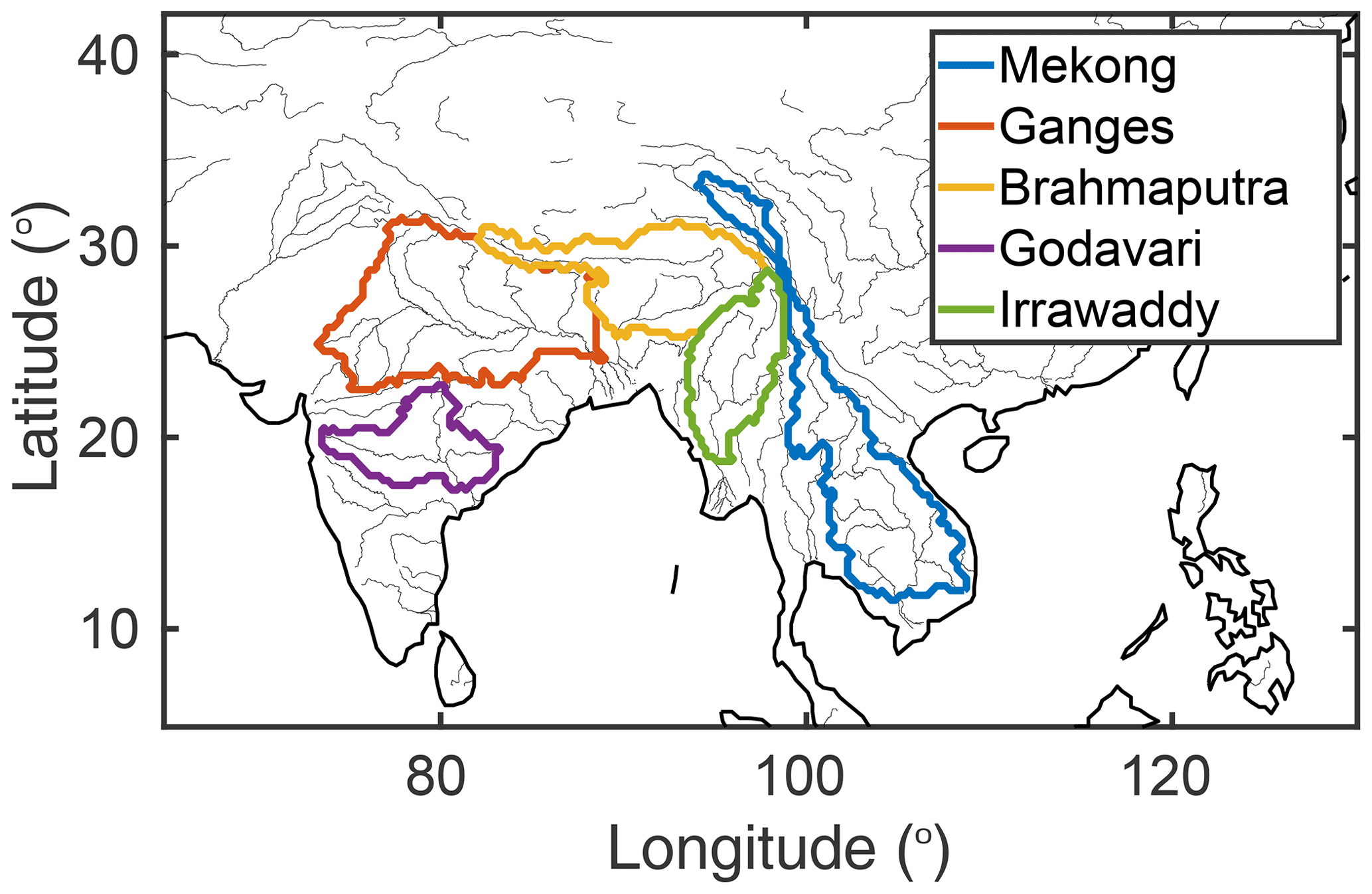
Figure 1 Five Himalayan basins considered in this study.

Given the limited availability of in situ data in the region, satellite observations are unique in their ability to monitor the dynamic of terrestrial waters (Tiwari et al., 2009; Papa et al., 2015; Salameh et al., 2017) and analyze their recent large-scale changes (Rodell et al., 2009; Asoka et al., 2017; Khaki et al., 2018). In particular, since 2002, the GRACE (Gravity Recovery and Climate Experiment) mission (Tapley et al., 2004) has monitored the mass gravity field variation and provided an estimation of TWSC at the monthly scale (for the period of 2002–2016), followed since 2018 by the Gravity Recovery and Climate Experiment Follow-On (GRACE-FO). However, the GRACE data time span is still too limited to study the long-term WC behavior related to climate changes or to human practices.

If classical approaches to retrieve total water storage (TWS) rely on land surface models (LSMs; Decharme et al., 2019b; Tootchi et al., 2019), studies have recently attempted to use instead statistical models fed with various climate drivers. For instance, Humphrey et al. (2017) have reconstructed the total water storage anomaly (TWSA) using a linear regression from precipitation and temperature, and Chen et al. (2019) have use an artificial neural network to reconstruct TWSA based on precipitation, temperature and surface variables (e.g., soil moisture and the normalized difference vegetation index – NDVI). Yang et al. (2018) reviewed and compared several statistical methods (linear, random forest, artificial neural network and support vector machine) to reconstruct TWSA from soil moisture, canopy water and snow water equivalent. These studies have focused on TWSA, without monitoring the whole WC. In fact, if statistical methods offer the opportunity to estimate TWS anomalies at a global scale in a simpler way than LSMs, they do not consider the water balance, and the related TWS estimate may not be coherent with the other water components.

Several studies have attempted to monitor the WC and provide independent estimates of TWSC using satellite observations (Lawford et al., 2007; Pan et al., 2012; Rodell et al., 2015; Munier and Aires, 2017; Tang et al., 2017). These analyses potentially allow new opportunities for WC monitoring over long time records in regions with limited access to in situ measurements. The use of satellite data to study the WC is however not straightforward. (1) Various datasets exist for the same geophysical variable, and (2) they all have uncertainties (systematic bias and random errors), which lead to (3) the inconsistency between an estimate of the same variable or among the variable estimates of the WC (Pellet et al., 2018). No singular estimate can be considered perfect, and many authors prefer to combine various available products (Sheffield et al., 2009; Sahoo et al., 2011; Azarderakhsh et al., 2011; Lorenz et al., 2014). For that purpose, some have focused on the water conservation equation:

$$\begin{array}{}\text{(1)}& \mathrm{\Delta }S=P-E-D,\end{array}$$

where ΔS is TWSC, P is precipitation, E is evaporation and D is discharge (expressed in mm per month, area-normalized). This closure of the WC budget allows for a better constraint of the integration of the datasets. For instance, Pan et al. (2012) have used an assimilation approach based on a Kalman filtering in the Variable Infiltration Capacity (VIC) model to derive a coherent analysis of the four terrestrial water variables (P, E, D and ΔS) at the basin scale, and Zhang et al. (2018) derive the methodology at a 0.5^∘ LSM pixel. Tang et al. (2017) implicitly use the water conservation through the Budyko model to estimate the long-term annual TWSC value based on P, E and R. This approach is not based on the assimilation of satellite observations but rather on the calibration of model parameters to match observed TWSC values. Rodell et al. (2015) used a 3D-VAR (variational) strategy to optimize the water cycle estimates at the global and annual scales.

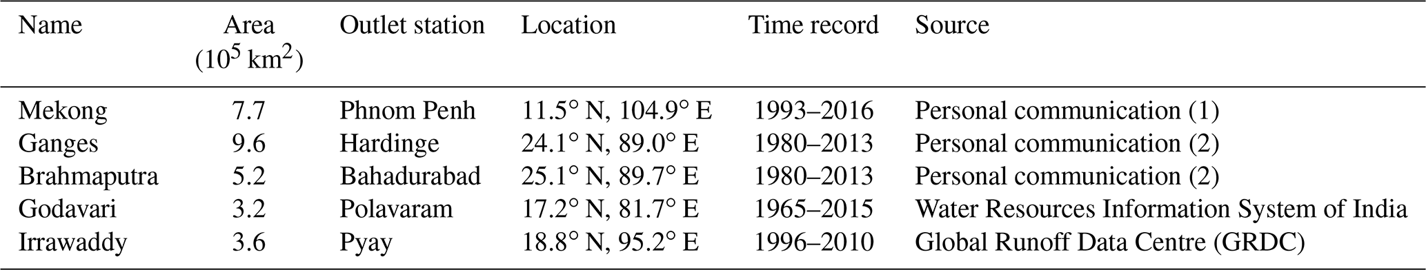
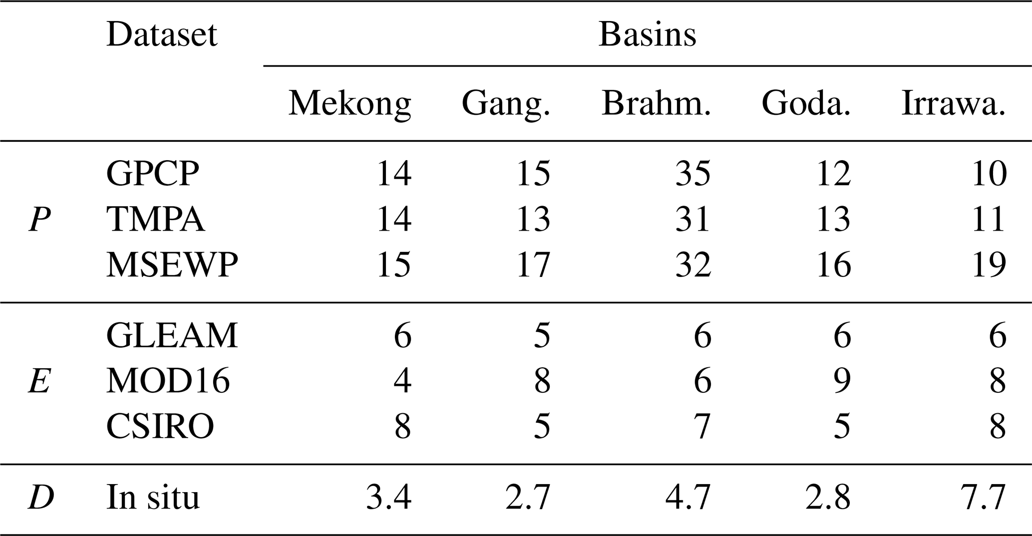
Table 1 Characteristics of the five considered basins and associate in situ measurement stations. (1) Personal communication with Sylvain Biancamaria. Data derived from radar altimetry water level estimations and calibrated against in situ measurements following a similar technique as in Papa et al. (2010). (2) Personal communication with the Bangladesh Water Development Board (BWDB; http://www.bwdb.gov.bd/, last access: 9 June 2020) as in Papa et al. (2012).

Other approaches perform this integration independently of any model, which allows the integrated datasets to be interesting for the calibration and validation of the model (Aires, 2014; Munier et al., 2014; Pellet et al., 2019). Pan and Wood (2006) and Aires (2014) have presented several methodologies to coherently integrate different hydrological datasets based on a budget closure. Munier et al. (2014) applied one of them (Aires, 2014) over the Mississippi basin using a remote-sensing observation for P, E and ΔS and an in situ measurement for D. The optimal integration is based on, first, a simple-weighting (SW) average and then, a closure post-filtering (PF) process. The SW + PF method improved the WC component estimate compared to the in situ observation. The uncertainties of the integrated product are reduced compared to the original datasets; the coherency is improved; and the residuals of the WC budget closure are decreased. Furthermore, the authors have developed a calibration approach based on the integrated product, able to correct each original estimate in an independent way. This calibration led to a significative reduction of the budget residual (see also Pellet et al., 2019). It was shown in Munier et al. (2014) that when three out of four WC components in Eq. (1) are available, the reconstruction of the missing one can be attempted. This is possible if the signal-to-noise ratio is sufficient: discharge reconstruction was not possible in Munier et al. (2014), but TWSC could be obtained in a very simple way, with results comparable in quality to a complex assimilation into a hydrologic model.

In this study, we propose to use this methodology to reconstruct the long-term evolution of TWSC over large southern Asian basins, based on satellite and in situ measurements and not a hydrological model. We denote this Satellite Water Cycle reconstruction “SAWC”. Section 2 introduces the tools used in this study, including a description of the region, the datasets used and the methodology. Section 3 presents the results and evaluations, while Sect. 4 draws the conclusions and perspectives.

2 Materials and methods

2.1 Basins

Table 1 lists the basins considered in this study. They are also represented in Fig. 1. They were defined by first choosing river discharge (D) in situ measurement stations close to the sea, over the major Himalayan rivers, with a long-enough time record. The HydroSHEDS (Hydrological data and maps based on SHuttle Elevation Derivatives at multiple Scales) topography (Lehner et al., 2006) was then used to determine the drainage area and basin delineation. The basins were selected based on the following factors: (1) their spatial domain needs to be large enough compared to the spatial resolution of the GRACE instrument, and (2) the river discharge measurements need to cover the GRACE period (2002–2015).

The following five basins were chosen:

• Mekong. The Mekong delta is one of the largest deltas in the world. It is a vast plain (55 000 km²) mostly lower than 5 m above sea level. Due to the seasonal variation in water level, the area presents extensive wetlands. The Mekong delta region that represents only 12 % of the total Vietnam area, allows ∼50 % of the annual rice production (up to three harvests per year in some provinces), ∼50 % of the fisheries and ∼70 % of the fruit production. Furthermore, questions related to oceanic water intrusions, the change of agriculture practices (e.g., number of rice harvest in 1 year), dam construction, ground water pumping and resulting land depletion all have an impact on TWSC and would therefore benefit from its monitoring.

• Ganges and Brahmaputra. The Ganges–Brahmaputra is the major river basin of the Indian subcontinent, supplying water to more than 700 million people. It covers an area of 1.7×10⁶ km², at the crossroad of Bangladesh, India, China, Bhutan and Nepal and is the third-largest freshwater provider to the world's oceans (after the Amazon and the Congo rivers) with a high influence on the regional climate. The basin is seasonally subject to the monsoon and faces strong climate variability between drought and flood periods. Furthermore, water management is an issue because of the increasing needs of the population and the demands for the industry and agriculture sectors. Thus, the freshwater supply leads to an overabstraction of groundwater stock during the dry season and then to a rapid fall of groundwater tables.

• Godavari. The Godavari River is the second-longest river in India after the Ganges, covering a total drainage area of ∼312 000 km² and accounting for nearly 9.5 % of the total geographical area of the country. It flows for a length of about 1465 km, from its origin near the Arabian Sea before falling out in to the Bay of Bengal, crossing several Indian states. The basin receives its maximum rainfall during the southwest monsoon, from June to September. The major part of basin is covered with agricultural land accounting for up to 60 % of the total area, while ∼3.5 % of the basin is covered by water bodies. The Godavari basin faces several hydroclimatic problems with a large portion of the basin being prone to drought, while flooding problems are common in its lower reaches, and its coastal areas are cyclone prone.

• Irrawaddy. Running over a length of 2100 km mainly within the boundaries of Myanmar, the Irrawaddy River is the most important river in the country. The basin takes up the northwestern part of Mainland Southeast Asia, with its source on the southern slopes of the Himalayas Mountains and emptying into the Andaman Sea of the Indian Ocean. The river basin area covers more than 400 000 km² and collects about two thirds of the surface water volume of Myanmar. It is subject to a tropical and subequatorial monsoon climate, and its hydrological regime, similarly to other large rivers of southern Asia, is fed with water on the slopes of the Himalayas Mountains, mainly from rains during the southwest-monsoon period and meltwater of glaciers. The river is vital for human activities, water supply and irrigation and hosts a high rate of biodiversity. It is prone to extreme events, such as floods from very heavy monsoon rains or extreme weather events like cyclones and severe droughts, and under climate change impacts, the region is facing major challenges for water resources.

2.2 Datasets

2.2.1 Datasets used in the integration

The datasets presented in this section will be used in the integration process to obtain an optimized description of the WC over the Himalayan basins. Most of them are satellite products. Only global satellite products have been considered. In order to integrate them, the datasets have been projected onto a common 0.25^∘ spatial resolution grid using a conservative interpolation (Jones, 1999) and resampled at the monthly scale.

• Precipitation (P). Three datasets based on remote-sensing observations have been selected. All are products calibrated using gauges measurements: the Global Precipitation Climatology Project (GPCP-V2; Adler et al., 2003), the Tropical Rainfall Measuring Mission Multi-satellite Precipitation Analysis (TMPA, 3B42-V7; Huffman et al., 2007) and the Multi-Source Weighted-Ensemble Precipitation (MSEWP) dataset (Beck et al., 2017). All these global datasets are widely used in the community. GPCP and TMPA use the same Threshold-Matched Precipitation Index (TMPI) algorithm to estimate instantaneous precipitation from multiple satellites by combining high-quality passive microwave observations and infrared data: their approaches differ only in the use of gauge analyses (Global Precipitation Climatology Center; GPCC) to obtain calibrated estimates. While TMPA is based on an inverse random-error variance weighting of the gauge data, GPCP assumes that the precipitation distribution estimated from the combined satellite estimates is optimal and uses the gauge observations only for debiasing. The MSEWP dataset merges the highest-quality precipitation data sources available as a function of timescale and location. It uses a combination of rain gauge measurements, the two previous satellite datasets and a reanalysis. These datasets have been compared in terms of uncertainties and performance in Sun et al. (2018). It should be noted that these datasets are not independent from each other but represent the best up-to-date precipitation estimates for hydrological studies.

• Evapotranspiration (E). Three satellite-based products were chosen to describe evapotranspiration over land. All these datasets are assumed to be satellite-based products, even if their retrieval algorithms can use auxiliary information and a model. The Global Land Evaporation Amsterdam Model (GLEAM-V3B; Martens et al., 2017; Miralles et al., 2011) uses the Priestley and Taylor (1972) empirical energy-based equation to calculate the reference evapotranspiration and separately estimate the different components of land evaporation: transpiration, bare-soil evaporation, interception loss, open-water evaporation and sublimation. GLEAM uses reanalysis (vA) or satellite (vB) precipitation inputs. The global observation-driven Penman–Monteith–Leuning (CSIRO; Zhang et al., 2016) evapotranspiration introduced by the Commonwealth Scientific and Industrial Research Organisation (CSIRO) and the MODIS Global Evapotranspiration Project (MOD16; Mu et al., 2011) are both evapotranspiration estimates based on the Penman–Monteith equations (Penman, 1948; Monteith, 1965). We choose these three datasets due to their different equations for evapotranspiration. The intercomparison of global evapotranspiration algorithms and datasets can be found in Michel et al. (2016).

• Total water storage change (TWSC; ΔS). The TWSC estimates are all based on the GRACE satellite measurements (Tapley et al., 2004). These estimates include the surface (wetland, floodplains, lakes, rivers and man-made reservoirs), soil moisture, snowpack, glaciers and groundwater waters. Satellite datasets are based either on the spherical decomposition of GRACE – for instance the Jet Propulsion Laboratory products (JPL; Watkins and Yuan, 2014) or the MASCON (mass concentration; MSC) solution: the JPL (Watkins et al., 2015) product that also includes a scaling factor for hydrological coherency. Another MASCON solution is offered by the Center for Space Research at the University of Texas, Austin (CSR). The CSR and JPL MASCON solutions differ in their processing: the JPL solution is based on an explicit estimation of mass anomalies at a specific mass concentration block location using the analytical partial derivatives of the inter-satellite range-rate measurements (Watkins et al., 2015). The CSR MASCON solution is first based on a spherical decomposition of the inter-satellite range-rate measurements that is truncated spatially at the location of the mass concentration (Save et al., 2016). The two solutions have been compared to the spherical solutions in terms of uncertainty in both min–max range and trend in Scanlon et al. (2016) and Save et al. (2016). We choose here the JPL solution because it is more independent of the spherical solution.

  Based on preliminary tests, it was observed that the MASCON solution for TWSC (ΔS) was in better agreement with the three other water component estimates and in particular over the Irrawaddy basin, compared to the spherical solutions. This could be due to the local inversion in the MASCON solution that prevents it from the destriping processing usually done in the spherical decomposition of GRACE. It as been shown that destriping could limit the capability of spherical solution over the particularly south–north-oriented basin (Wahr et al., 2006; Rateb et al., 2017). In the following, the JPL MASCON solution is used. Figure 2 represents the GRACE TWSC and TWSC anomaly (with respect to the averaged season computed over the 2002–2015 period), over the five basins of the previous section. The annual cycle is well pronounced in each basin, showing the strong seasonality of the WC in these regions. The anomalies have strong inter annual variations showing the evolution of the WC along the years.

• Discharge (D). The Global Runoff Data Centre (GRDC) gathers discharge measurements at the global scale. However, for large tropical rivers and more particularly over southern Asia, only a few stations are available, and they are not all updated to recent periods. In particular, among the five considered rivers of this study (Fig. 1), four of them are not available with GRDC data, and we obtained them instead from personal communication and collaboration with local colleagues (Table 1).

In the following, an a priori specification of the uncertainties for each one of these satellite sources is required. Such characterizations are generally specific to the product and site. Some studies (Pan et al., 2012; Sahoo et al., 2011; Zhang et al., 2018) estimate the a priori uncertainty of particular water components based on the spread among the various estimates (taking the spread of estimates as an estimate of the uncertainties can sometimes be dangerous). In our case, this approach would not take into account the fact that the precipitation estimates are not independent. The values used here are derived from Munier et al. (2014), in which the authors reviewed carefully the literature on this topic. The partitioning of uncertainty between P and E has however been modified to allow for larger uncertainty in P, since datasets are dependent in our case. As the objective of the current study is to reconstruct GRACE TWSC, the approach assumes lower errors in the GRACE estimate that becomes our reference. For the three precipitation datasets, we specify a 14 mm per month SD (standard deviation) error. Similarly, for three evapotranspiration datasets, we specify a 7 mm per month SD. River discharge is an in situ measurement, so a 3 mm per month SD is chosen. Since the objective is the reconstruction of the GRACE observations over long time series, we specify a small uncertainty (1 mm per month) to avoid changing these values during the integration.

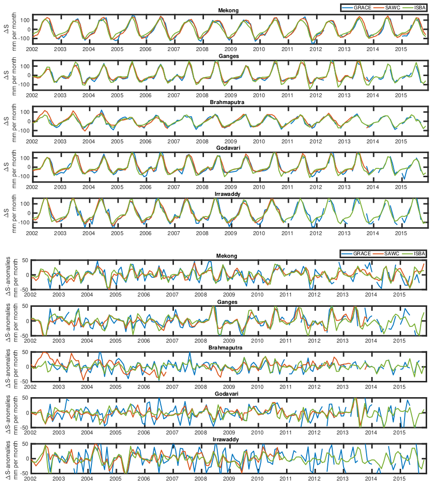
Figure 2 TWSC (top panels) and TWSC seasonal anomaly (bottom panels) for the three estimates (GRACE, SAWC and ISBA) for the five Himalayan basins over the GRACE time period.

2.2.2 Datasets used in the evaluation

• ISBA hydrological model. To evaluate our reconstruction of the long-term evolution of TWSC over large Himalayan basins, we also use the ISBA-CTRIP (Interactions between Soil, Biosphere and Atmosphere CNRM – Centre National de Recherches Météorologiques – Total Runoff Integrating Pathways) numerical land surface system. ISBA-CTRIP is a “state-of-the-art” hydrological system that simulates TWSC at the global scale with a good accuracy, as shown in Decharme et al. (2019a). The ISBA-CTRIP TWSC data provide all water mass variations (river water mass and floodplains, snowpack, canopy water, total soil moisture and groundwater storage). The ISBA land surface model explicitly solves the energy and water budgets at the land surface at any time step. The CTRIP river routing model simulates river discharges up to the ocean from the total runoff computed by the ISBA model. A two-way coupling between the ISBA and CTRIP models allows one to account for (1) a dynamic river flooding scheme with explicit interactions between the floodplains, the soil and the atmosphere (through free-water evaporation, precipitation interception and infiltration) and (2) a 2D diffusive-groundwater scheme to represent unconfined aquifers and upward capillarity fluxes into the superficial soil. More details can be found in Decharme et al. (2019a). In this study, we use a product derived from a global offline simulation at 0.5^∘ resolution done with this ISBA-CTRIP configuration and driven at a 3-hourly timescale by the ERA-Interim (ECMWF Reanalysis) reanalysis over the 1979–2015 period. To ensure that realistic precipitation is fed to the ISBA-CTRIP system (Szczypta et al., 2014), the ERA-Interim precipitation is, here, hybridized to match the monthly values from the gauge-based Global Precipitation Climatology Center (GPCC) Full Data Product V6 (Schneider et al., 2011, 2014). At each time step, ISBA-CTRIP gives the variation of the total mass of water. The TWSC estimate from ISBA-CTRIP is then the monthly average of this field, which is slightly different than the reconstruction via Eq. (1) (see Appendix A). Since GRACE data are anomalies relative to a reference geoid, the TWSC estimate from ISBA-CTRIP is also calculated in terms of the anomaly over the analyzed period. To be consistent with the GRACE data, the simulated TWS values were smoothed using a 200 km wide Gaussian filter, which is quasi-similar to the filter used for the GRACE products (Watkins et al., 2015). In the following, ISBA-CTRIP is shortened in the ISBA model.

• GLDAS hydrological model. For the purpose of comparison, we also use the Noah 2.7.1 land hydrology model of the Global Land Data Assimilation System (GLDAS). Its purpose is to ingest satellite- and ground-based observations using advanced land surface modeling and data assimilation techniques, in order to generate optimal fields of land surface states and fluxes. GLDAS is an uncoupled land surface modeling system that drives multiple models, runs globally at the resolution of 0.25^∘ and produces results in near-real time. The GLDAS system is described in Rodell et al. (2004). GLDAS is a platform of assimilation and differs from hydrological models. In particular, they do not model reservoirs. For our comparison, we use the land water content output of GLDAS.

These two global and well-known models have been chosen for comparison, even if neither of them includes anthropogenic effects on the river discharge and groundwater storage. Significant efforts have been made during the last 2 decades to incorporate anthropogenic impacts in an LSM (Hanasaki et al., 2006; Haddeland et al., 2014), but crucial challenges still remain. Most of these new schemes in LSMs have been developed and used offline for regional-scale studies and without a common and standardized framework (Pokhrel et al., 2016; Döll et al., 2016). At a global scale, the state of the art does not include the global representation of flow regulation and irrigation water needs.

2.3 Methodology

The notations are presented in this section, but more methodological details can be found in Aires (2014). The last version of the integration methodology is well described in Pellet et al. (2019).

2.3.1 Water cycle budget closure at the basin scale

The first step of the integration process consists of merging the various datasets presented in Sect. 2.2.1. The simple-weighting estimate (i.e., ensemble mean) is used to describe each water component based on all the available datasets (Aires, 2014):

$$\begin{array}{}\text{(2)}& P_{\mathrm{SW}}={\displaystyle \frac{\mathrm{1}}{p-\mathrm{1}}}\sum _{i=\mathrm{1}}^p{\displaystyle \frac{\sum _{k\ne i}{\left({\mathit{\sigma }}_k\right)}^{\mathrm{2}}}{\sum _k{\left({\mathit{\sigma }}_k\right)}^{\mathrm{2}}}}{P}_i,\end{array}$$

where P_SW is the simple-weighting estimate, p is the number of precipitation inputs P_i, σ_i is the standard deviation of the input P_i and P_i is the ith precipitation inputs. This equation is valid when there is no bias error in the P_is (thanks to a preliminary bias correction) and is optimal when the errors ϵ_i are statistically independent from each other. This expression is valid for the other water components. The variance of the P_SW uncertainties is then given by

$$\begin{array}{}\text{(3)}& {\mathit{\sigma }}_{P_{\mathrm{SW}}}={\displaystyle \frac{\mathrm{1}}{(p-\mathrm{1}{)}^{\mathrm{2}}}}\sum _{i=\mathrm{1}}^p{\left({\displaystyle \frac{\sum _{k\ne i}{\left({\mathit{\sigma }}_k\right)}^{\mathrm{2}}}{\sum _k{\left({\mathit{\sigma }}_k\right)}^{\mathrm{2}}}}\right)}^{\mathrm{2}}{\mathit{\sigma }}_i^{\mathrm{2}}.\end{array}$$

A similar approach is used for the three estimates of evapotranspiration. Following the error specification in Sect. 2.2.1, the uncertainty of the precipitation (evapotranspiration) merged estimate is characterized by an 8 mm per month SD (4 mm per month SD). Only one discharge dataset is available, and only the MASCON-JPL is used for TWSC. We denote X_SW=(P_SW, E_SW, D_SW, ΔS_SW), where SW stands for the simple weighting the results of the merging.

Following Aires (2014), it is then possible to write the conservation of water mass at the basin scale as a constraint applied on the state vector X=(P, E, D, ΔS). The WC budget constraint is expressed in Eq. (4). A relaxed constraint is considered (Pellet et al., 2019): the WC budget is closed within an error r that follows a normal distribution with specified uncertainty (Yilmaz et al., 2011). The problem can be written in the following way:

$$\begin{array}{}\text{(4)}& {\displaystyle }\begin{array}{rl}& X^{\mathrm{t}}=(P,E,D,\mathrm{\Delta }S)\\ & G=[\mathrm{1},-\mathrm{1},-\mathrm{1},-\mathrm{1}]\\ & X^t\cdot G^{\mathrm{t}}=r\mathrm{with}r\sim \mathcal{N}(\mathrm{0},\mathrm{\Sigma }),\end{array}\end{array}$$

where ^t is the transpose sign, G is the closure operator and Σ is the variance of the relaxation r. The optimized solution of this problem can be expressed as

$$\begin{array}{}\text{(5)}& X_{\mathrm{PF}}=\left(I-K_{\mathrm{PF}}\cdot G{\mathrm{\Sigma }}^{-\mathrm{1}}{G}^{\mathrm{t}}\right)\cdot X_{\mathrm{SW}},\end{array}$$

where $K_{\mathrm{PF}}=({\mathbf{B}}^{-\mathrm{1}}+G{\mathrm{\Sigma }}^{-\mathrm{1}}{G}^{\mathrm{t}}{)}^{-\mathrm{1}}$, in which PF stands for the post-filtering process of the previous solution X_SW and B is the a priori error covariance matrix of X_SW that is specified here as

$$\begin{array}{}\text{(6)}& \mathbf{B}={\left(\begin{array}{cccc}\mathrm{8}& \mathrm{0}& \mathrm{0}& \mathrm{0}\\ \mathrm{0}& \mathrm{4}& \mathrm{0}& \mathrm{0}\\ \mathrm{0}& \mathrm{0}& \mathrm{3}& \mathrm{0}\\ \mathrm{0}& \mathrm{0}& \mathrm{0}& \mathrm{1}\end{array}\right)}^{\mathrm{2}}.\end{array}$$

This methodology allows for obtaining a solution X_PF that closes the WC budget (within the relaxation r).

2.3.2 The calibration for the temporal extension of the closure constraint

An important limitation of the closure integration is the need for a common coverage period for all sources of information used in the integration. The optimized dataset cannot be provided for time steps with a missing component. To overcome this issue, a calibration to independently correct each water component towards the closure solution has been introduced (Munier et al., 2014). This calibration is based on a statistical regression between the merged observations X_SW and the optimized estimates X_PF, assuming that this optimized dataset represents the reference. In Pellet et al. (2019), the calibration is not strictly linear in order to avoid correcting null water fluxes (Munier and Aires, 2017). The following regression is used for P, E and D:

$$\begin{array}{}\text{(7)}& X_{\mathrm{CAL}}=a\cdot X_{\mathrm{SW}}+b\cdot \left(\mathrm{1}-e^{\frac{-X_{\mathrm{SW}}}{c}}\right)\end{array}$$

so that X_CAL becomes closer to X_PF. This calibration is close to a linear calibration, but zero values are kept unchanged. The variables a, b and c are the calibration parameters. The calibration is performed not only during the GRACE period (2002–2015) but also over the complete record of each satellite dataset. It was shown in previous studies that the calibration does not allow for a perfect balance of the WC, but it greatly reduces the WC budget residuals compared to the original estimates.

The calibration of Eq. (7) is applied independently on each dataset of Sect. 2.2.1. Table 2 shows the original (X_SW) versus the calibrated (X_CAL) root mean squares of the WC budget residuals. It can be seen that the calibration has a significant improvement in each basin, with a decrease of the error from 25 % (over the Ganges) to 54 % (over the Brahmaputra).

Table 2 Root mean square of the WC budget residuals (in mm per month) for the original (X_SW) and the calibrated (X_CAL) estimates over the five considered basins.

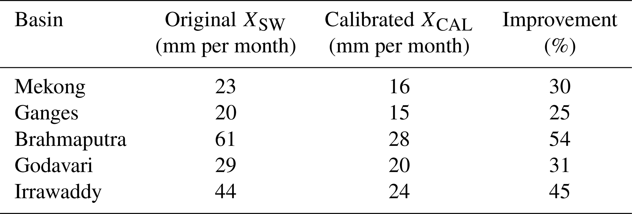
Figure 3 compares in rows the original (X_SW) and calibrated (X_CAL) estimates of the four water components with the WC budget residuals for the Ganges and the Brahmaputra basins over the GRACE period. It can be seen that for the Ganges, the water components are not particularly impacted by the calibration. This is due to the overall coherency of the various water components estimates and the relatively low WC budget residual for this particular basin. Only a small improvement can be noticed in the WC budget residuals. For the Brahmaputra basin, precipitation and evapotranspiration are much more impacted by the calibration. The discharge is slightly changed because we specified a low uncertainty on this in situ variable (i.e., SD = 1 mm per month). The resulting WC budget residuals are much smaller for the calibrated solution, meaning that this solution is more coherent hydrologically.

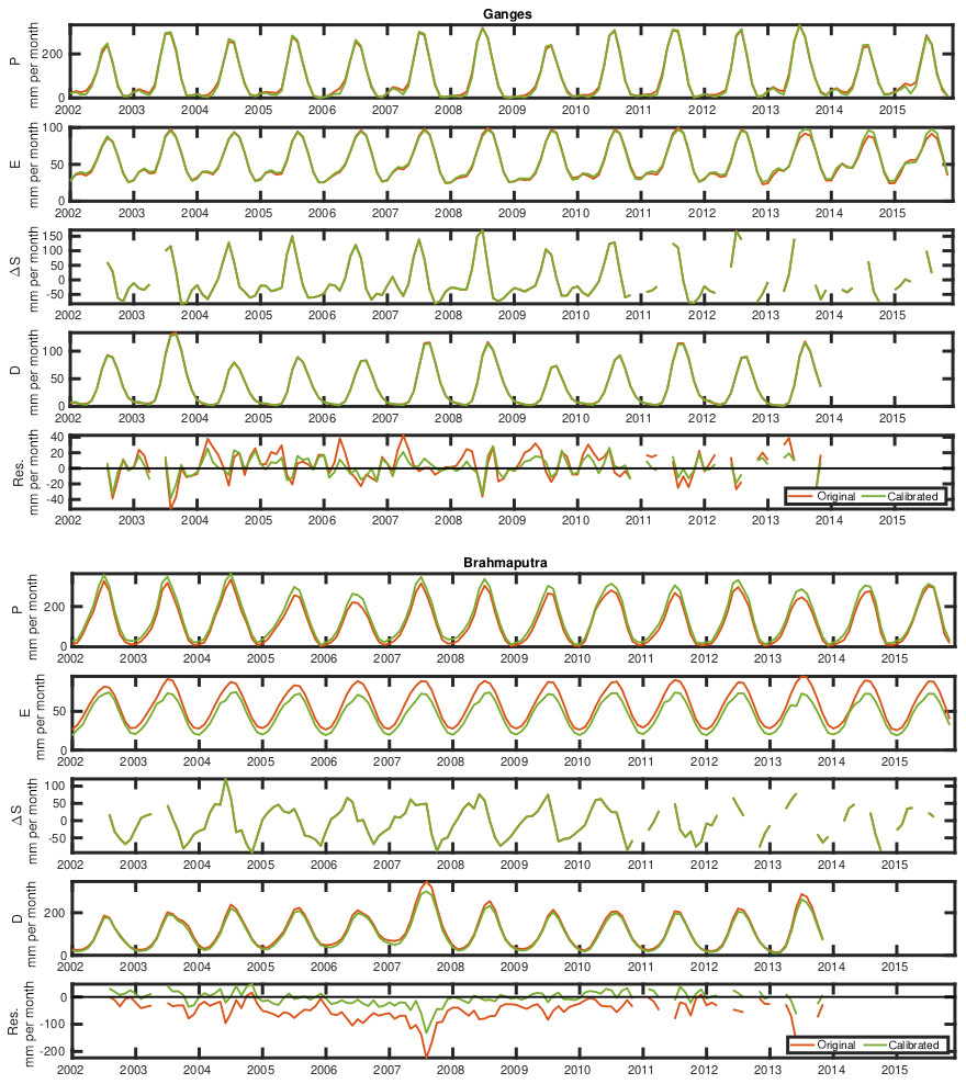
Figure 3 Comparison of the four water components estimates and the WC budget residuals (in rows) for the original (X_SW, red) and calibrated (X_CAL, green) estimates. The estimates are for the Ganges (top panels) and the Brahmaputra (bottom panels) basins. The last row of each panel depicts the residual (Res.) of the water budget for these basins.

2.3.3 Satellite Water Cycle (SAWC) reconstruction

Similarly to Munier et al. (2014), the three available water components (P, E and D) are used to estimate the fourth one, TWSC ΔS. This allows extending temporally the monitoring of TWSC before and after the GRACE period (2002–2015). In addition, the GRACE satellite has been down for maintenance every 6 months since 2011. The calibration approach allows for filling gap measurements in the GRACE observation with high accuracy (Munier et al., 2014). Following Landerer et al. (2010) and to avoid temporal mismatching between GRACE-derived TWSC and the monthly estimate of the other water components, we use centered differences of the mean TWS anomalies to compute TWSC ΔS(t). The right-hand side of Eq. (1) is therefore computed for each month t as

$$\begin{array}{}\text{(8)}& \mathrm{\Delta }S\left(t\right)={\displaystyle \frac{\mathrm{1}}{\mathrm{4}}}{X}_{\mathrm{CAL}}^{\prime }(t-\mathrm{1})+{\displaystyle \frac{\mathrm{1}}{\mathrm{2}}}{X}_{\mathrm{CAL}}^{\prime }\left(t\right)+{\displaystyle \frac{\mathrm{1}}{\mathrm{4}}}{X}_{\mathrm{CAL}}^{\prime }(t+\mathrm{1}),\end{array}$$

where $X_{\mathrm{CAL}}^{\prime }=(P_{\mathrm{CAL}}-E_{\mathrm{CAL}}-D_{\mathrm{CAL}})$ and ΔS is the centered mass rates

$$\begin{array}{}\text{(9)}& \mathrm{\Delta }{S}_t={\displaystyle \frac{S(t+\mathrm{1})-S(t-\mathrm{1})}{\mathrm{2}}}.\end{array}$$

2.3.4 Uncertainty characterization

Estimating product uncertainty is valuable information for instance in an assimilation framework. Most uncertainty estimation approaches require defining first a reference: in situ, reanalysis or a consensus of all available data. In this work, the chosen reference is the optimized product (X_PF); this is a solution that is hydrologically more coherent and reliable than the original datasets. All original satellite datasets are compared to this reference to compute bias (not shown) and uncertainty (standard deviation) errors. For instance, for precipitation: ${\mathit{\sigma }}_{\mathrm{P}}^{\mathrm{2}}=E\left[\right(P-P_{\mathrm{PF}}{)}^{\mathrm{2}}]$. Such an approach was used in Munier and Aires (2017) and Pellet et al. (2019).

Table 3 gathers the a posteriori uncertainty estimates (computed as the distance between the original datasets and the reference) for all the original satellite datasets for P, E and D over the five considered basins. These a posteriori uncertainty estimates are in line with the specifications that were taken a priori for each of the datasets (Sect. 2.2.1). It can be seen that the Brahmaputra has higher uncertainties, especially for precipitation. MSEWP appears less reliable than GPCP or TMPA for precipitation; and GLEAM seems more reliable than MOD16 or CSIRO over these five basins.

Table 3 Uncertainty estimates (in mm per month) in terms of SD error compared to X_PF for P, E and D over the five considered basins for the original datasets. Gang.: Ganges; Brahm.: Brahmaputra; Goda.: Godavari; Irrawa.: Irrawaddy.

It is possible to compute the SAWC reconstruction of TWSC based on Eq. (10). Once calibrated, P_CAL, E_CAL and D_CAL estimates are available over a long time period. They can be used to infer ΔS using the WC budget equation (Eq. 1), before and after the GRACE period:

$$\begin{array}{}\text{(10)}& \mathrm{\Delta }{S}_{\mathrm{SAWC}}=P_{\mathrm{CAL}}-E_{\mathrm{CAL}}-D_{\mathrm{CAL}}.\end{array}$$

The reconstruction of TWSC has a different temporal coverage for the five basins because D (and then D_CAL) availability varies (see Table 1). The measurement errors of P, E and D of Table 3 are assumed to be independent and normally distributed. In this case, the error in the SAWC reconstruction of ΔS is given by

$$\begin{array}{}\text{(11)}& {\mathit{\sigma }}_{\mathrm{\Delta }S}^{\mathrm{2}}={\mathit{\sigma }}_{\mathrm{P}}^{\mathrm{2}}+{\mathit{\sigma }}_{\mathrm{E}}^{\mathrm{2}}+{\mathit{\sigma }}_{\mathrm{D}}^{\mathrm{2}},\end{array}$$

where σ_P, σ_E and σ_D are the a posteriori uncertainty merged estimate using Eq. (3) with the values of a posteriori estimate in Table 3.

3 SAWC reconstruction of TWSC and evaluation

3.1 Evaluation over the GRACE period (2002–2015)

The resulting SAWC time series can be observed (red) and compared to GRACE measurements (blue) over the 2002–2015 period in Fig. 2, over the five basins, for the raw and the anomalies. The ISBA simulation is represented too (green). The seasonality is well represented in every estimate. The specific seasonality of each basin is well characterized by the SAWC reconstruction; see for instance the difference between the Mekong and the Brahmaputra seasons. The SAWC reconstruction uses the GRACE data to calibrate the other datasets, but once the P, E and D calibrations are done, the SAWC data in Eq. (10) do not use the GRACE data anymore. This is a good demonstration that GRACE-compatible TWSC estimates can be obtained from the other water components. The rich interannual signal in the anomalies is well captured too by SAWC times series. Some extreme years are well captured, e.g., the high extremes of the 2008 year over the Ganges basin, which are depicted also by the ISBA model.

In order to quantify the agreement of these times series, Fig. 4 represents the correlation, the correlation of the anomaly and the root mean square of the difference (RMSD) between the four estimates (GRACE, SAWC, ISBA and GLDAS) over the five Himalayan basins for the GRACE period (2002–2015). It can be see that the SAWC times series is more highly correlated (0.96 on average) with the GRACE data than the ISBA data (0.94); GLDAS has a much lower agreement with GRACE (0.91) because it misses completely the season in the Irrawaddy basin for some years (not shown for clarity in Fig. 2). Again, it is not surprising that the SAWC value is close to GRACE because it has been designed to do that.

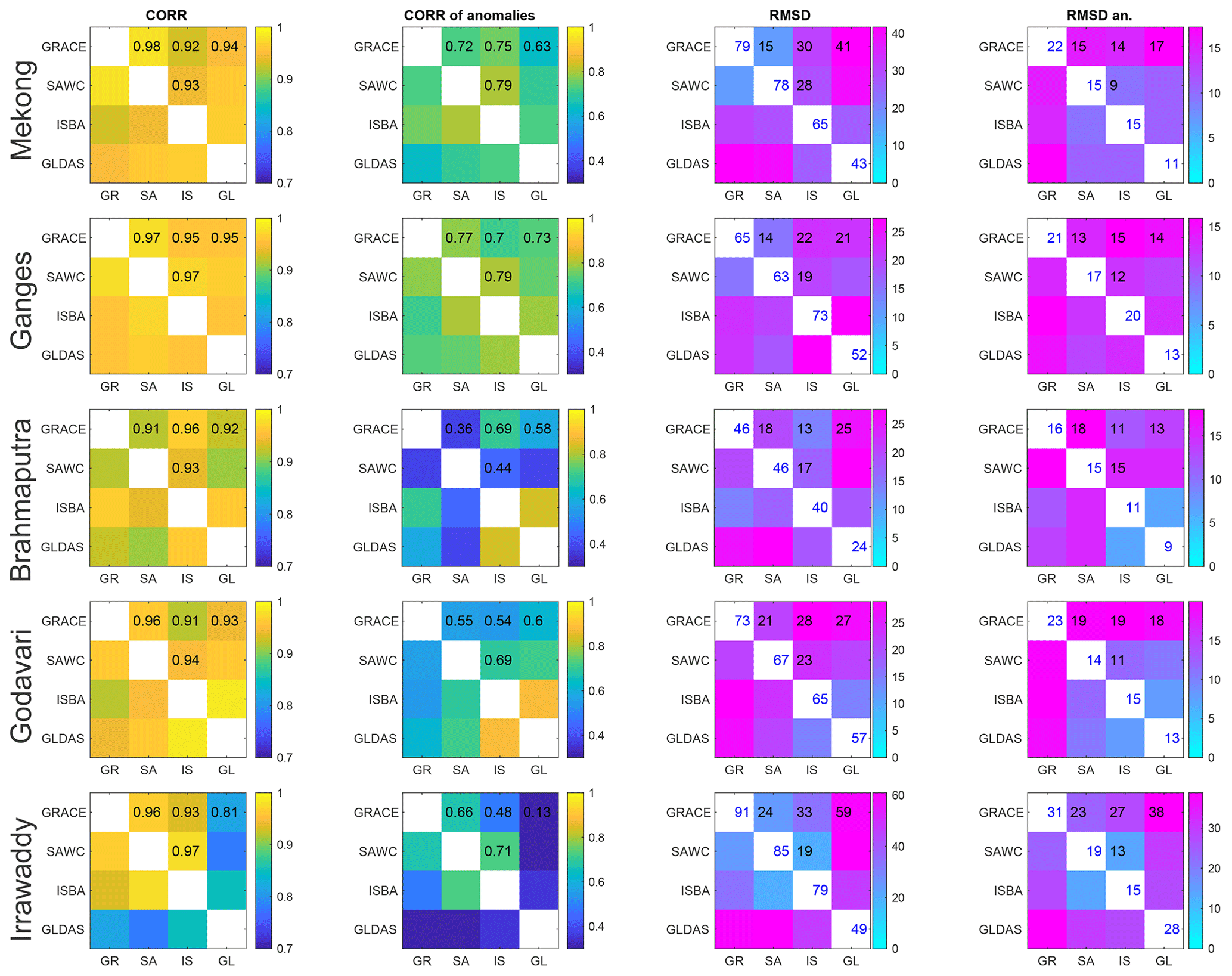
Figure 4 The correlation (CORR; left panels), the correlation of the anomalies (CORR of anomalies; center-left panels), the root mean square of the difference (RMSD; center-right panels) and the root mean square of the difference of the anomalies (RMSD an.; right panels) between the four estimates (GRACE, SAWC, ISBA and GLDAS; abbreviated as GR, SA, IS and GL on the x axis) for the five Himalayan river basins (in rows) over the GRACE period (2002–2015). Some of the commented statistics are also indicated numerically.

In terms of the correlation of anomalies, the SAWC estimate is always closer to the ISBA estimate than to GRACE, even if the SAWC estimate has a high correlation of anomalies with GRACE (between 0.69 and 0.79) except over the Brahmaputra basin (0.36). This will be analyzed below. Comparatively, a GLDAS estimate is less correlated with GRACE over the four basins (except Brahmaputra basin). The RMSD and RMSD values of anomalies show a pattern similar to that of the correlation values over all the basins. The RMSD statistics are better for the SAWC (19 mm per month error) than for the ISBA model (26 mm per month error), but this is no surprise because the season is a large part of these discrepancies. GRACE has a low spatial resolution (300 km² at the Equator); this can decrease the accuracy of the TWSC anomaly estimates over small basins (e.g., Godavari or Irrawaddy). The smaller the basin is, the larger the gap between the SAWC-GRACE and SAWC-ISBA correlation becomes. The SAWC estimate is based on precipitation and evapotranspiration obtained at a finer spatial resolution (0.25^∘) than GRACE. Therefore, the SAWC value, as the ISBA value (at the 0.25^∘ spatial resolution), represents better the anomaly over small basins as long as precipitation and evapotranspiration are accurate enough. Over the Brahmaputra basin, the large uncertainty of satellite evapotranspiration products over the mountains (see the impact of the calibration for the evapotranspiration estimate over this basin in Fig. 3) might impact the SAWC TWSC accuracy and explain why GLDAS and the ISBA model are better over this basin. This assumption is later confirmed in Fig. 6, in which precipitation in ISBA and SAWC values are close but the anomalies of E differ. Overall, it can be concluded that the SAWC values seems closer to GRACE than ISBA for some events, as seen in the anomalies over the Brahmaputra basin. GLDAS has a lower agreement with ISBA, in particular over the Irrawaddy basin. The discrepancy between simulated TWSC from ISBA and GLDAS can be explained by the different representation of aquifers in these two models. While a 2D diffusive-groundwater scheme in ISBA represents unconfined aquifer processes (Vergnes and Decharme, 2012; Vergnes et al., 2012), the Noah land model used in the GLDAS simulations did not include surface and groundwater storage. Therefore, the simulated mean seasonal cycle and the interannual variability of TWSC is improved in ISBA (Decharme et al., 2019b). On the contrary, deviations from GRACE TWSC can thus be expected with GLDAS (Syed et al., 2008). Based on these results, the SAWC solution is compared only to ISBA in the following over the long time period.

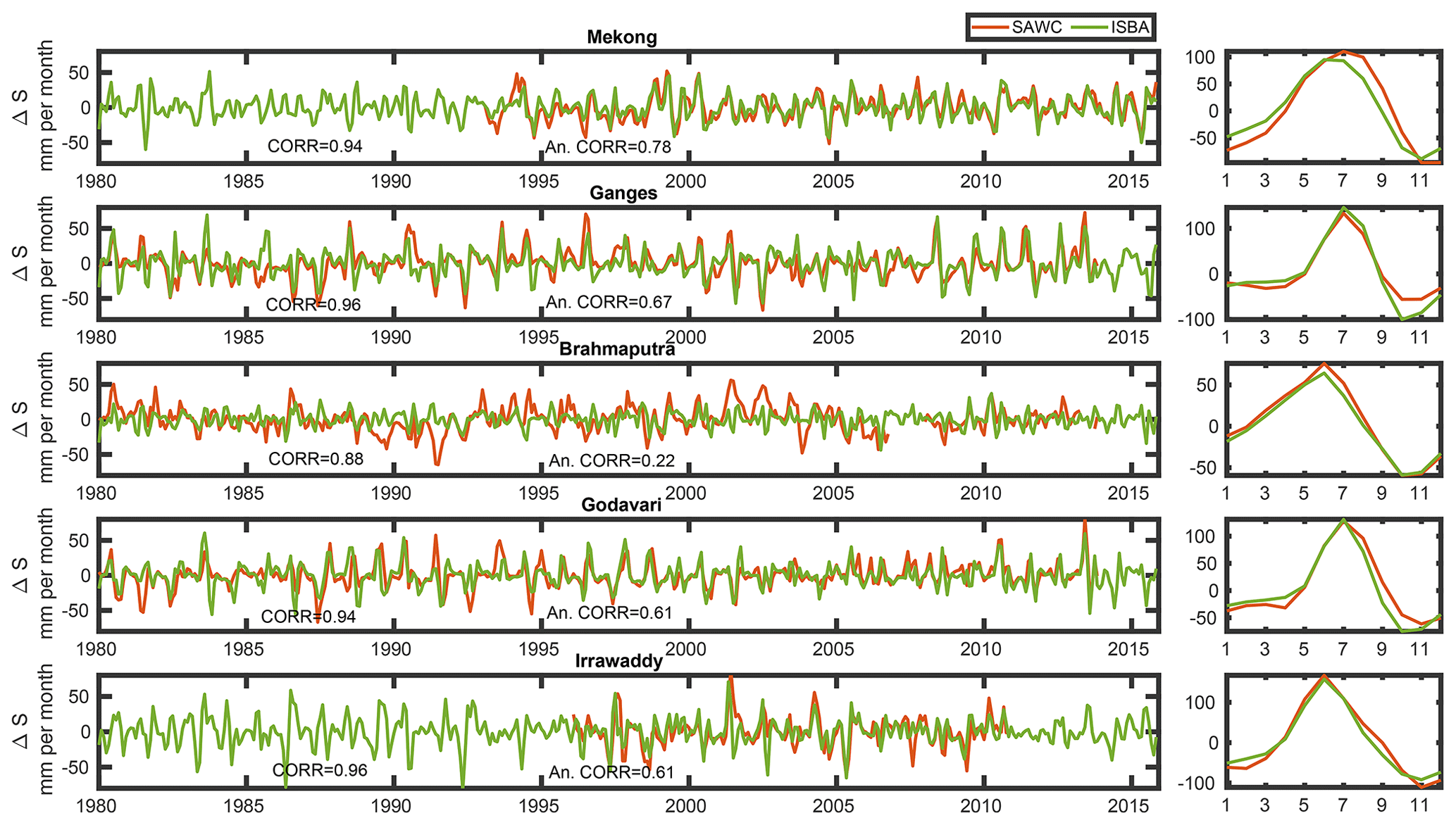
Figure 5 Times series of TWSC (left panels) and the seasonal cycle (right panels) from 1980 to 2015 for the SAWC and ISBA model estimates over the five considered basins. Correlations of raw (CORR) and anomaly (An. CORR) values are also provided.

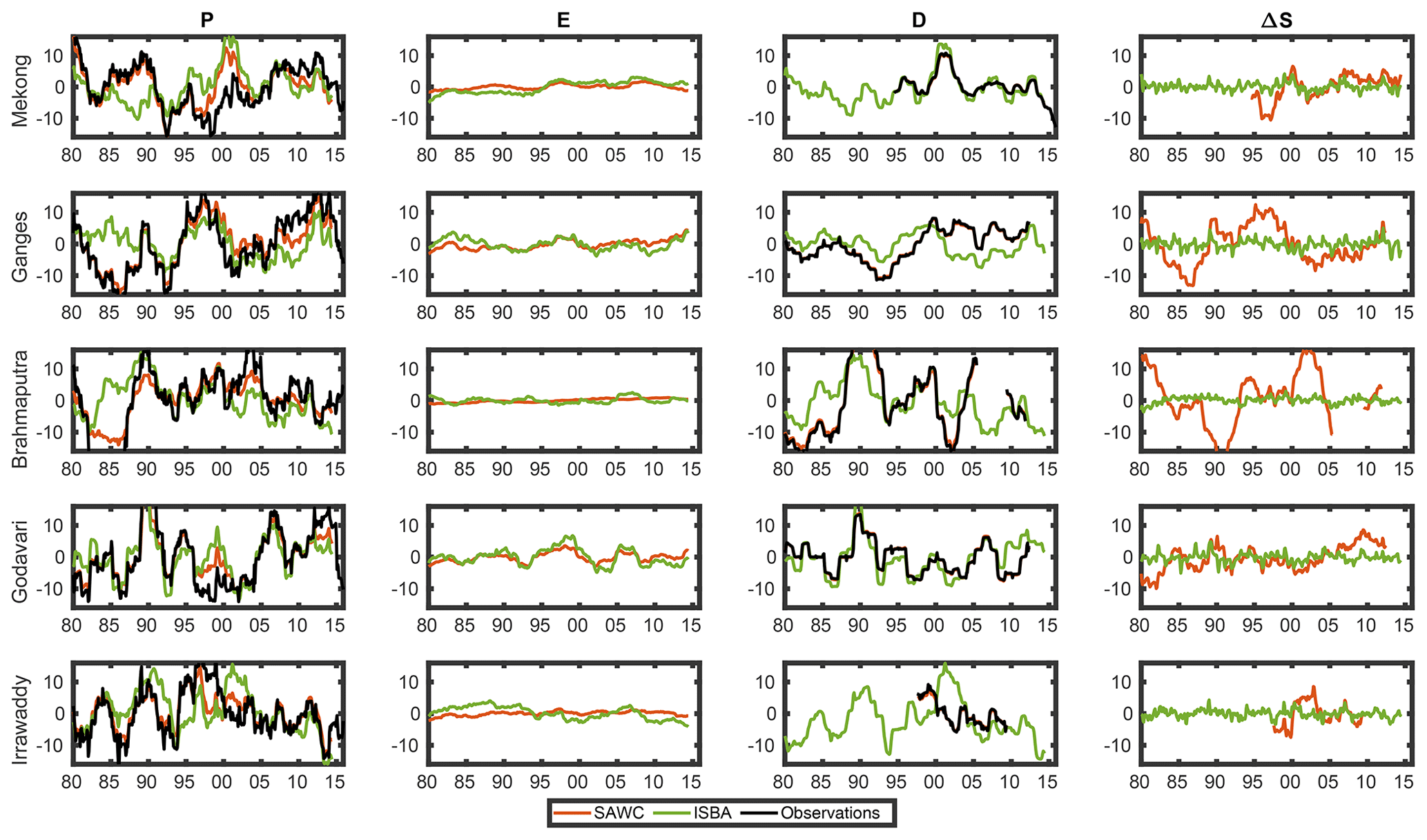
Figure 6 Times series of the WC components (in mm per month) for 1980–2015 in terms of anomalies (with respect to the climatological season) smoothed using a 3-year moving window for the five considered basins for the SAWC (red) and ISBA (green) estimates. Observations are also represented in black (MSEWP for P and in situ measurements for D).

3.2 Comparison with ISBA TWSC

In Fig. 5, the SAWC reconstruction is compared to the ISBA simulation over a long time record. ISBA is available from 1980 to 2015; the SAWC reconstruction is available based on the river discharge in situ measurements coverage (see Table 1). The first important remark to be made regards the very good seasonal cycle agreement between the SAWC and ISBA values: correlations are larger than 0.93, except for the Brahmaputra with a correlation of 0.88. This basin presents a particular water cycle in 2007 that is analyzed in Appendix (Fig. B1). In the following, the year 2007 has been removed from the comparison analysis. For the Ganges basin, the main difference between the two estimates is that ISBA represents larger negative seasonal peaks and a slight phase in the seasons over the Mekong. In terms of seasonal anomalies, the agreement is also satisfactory with correlations between 0.61 (Godavari and Irrawaddy) and 0.78 (Mekong is always well represented in our analysis), except again for the Brahmaputra (correlation of 0.22). However, based on the 2007 analysis over the Brahmaputra (Fig. B1), we believe that the SAWC anomalies might be more reliable because they use measured in situ D values as compared to the models.

In Fig. 6, we analyze the long-term TWSC time series in terms of anomalies with respect to the climatological season. Furthermore, the times series of these anomalies have been smoothed using a 3-year moving window. For instance, a peak value of 10 mm per month means that the time series was on average 10 mm higher than the climatological season for 3 consecutive years (i.e., 360 accumulated millimeters in 3 years).

In general, the SAWC model reproduces well the long-term anomalies of the MSEWP precipitation dataset. This satellite dataset was used as input with two close other products (TMPA and GPCP calibrated using the same precipitation gauges) for the SAWC reconstruction (while ISBA uses a mix between GPCC and the ECMWF reanalysis; see Sect. 2.2.2). In general, ISBA precipitation inputs have some differences with MSEWP during the 1980s and in 2010–2015; this requires further investigations beyond the scope of this study. The evapotranspiration anomalies are relatively flat for all basins, except for the Godavari, where both the SAWC and ISBA values are in good agreement. By construction, the discharge D measurements are well reproduced by the SAWC reconstruction, but some significant differences can be observed for the ISBA model. These important temporal variations of the D anomalies have an important impact on the other WC components of the SAWC reconstruction. TWSC anomalies ΔS have a rather constant behavior in the ISBA analysis, but large variations are present in the SAWC reconstruction. For instance, there is a large water deficit in 1990–1991 over the Brahmaputra or over the Ganges in 1985–1887.

From this comparison, the following conclusions can be drawn. When precipitation from the SAWC reconstruction matches well precipitation used to force ISBA, discharge simulated by ISBA is quite close to in situ measurements (discharge from the SAWC reconstruction), as well as for the Mekong and the Godavari basins, which could be seen as an indicator of the good quality of P_SAWC. On the contrary, the main differences between D_ISBA and D_SAWC are either due to large differences of precipitation amounts or to the TWSC dynamics. In ISBA, the groundwater storage is a simple delayed reservoir (with a constant delay parameter) which tends to attenuate the river dynamics. It is then not able to simulate long-term groundwater dynamics (Pedinotti et al., 2012). Moreover, the ISBA model does not represent anthropogenic factors such as groundwater extraction, river regulation or irrigation, which may significantly impact river discharges. For instance, in Fig. 6, the Mekong River discharge anomalies show a lower min–max range in the observations than in ISBA. Li et al. (2017) highlight the impact of the construction of the Xiaowan and the Nuozhadu dams starting in 1991. The dam reduces the streamflow in particularly wet seasons and increases the streamflow in particularly dry seasons, which lowers the anomaly variations. For this basin, D is more correlated to precipitation in ISBA (0.94) than in the SAWC (0.63) solutions. This shows that modeled D is more straightforwardly dependent of the precipitation than in observations. On the contrary, the TWSC anomaly is less linked to precipitation in the ISBA model than in the SAWC model, where natural recharge is better represented. This difference is also discussed in Appendix A. The integration of anthropogenic processes are currently under development, as are alternatives like data assimilation (Emery et al., 2018; Albergel et al., 2017).

3.3 Indirect evaluation using the GIEMS inundation area

An important component of TWS corresponds to the surface waters. The GIEMS (Global Inundation Extent from Multi-Satellites) database provides an estimation of the inundation extent from 1993 to 2007, at the global scale, on a 0.25^∘ resolution equal-area grid (Prigent et al., 2007). GIEMS was fully assessed over Asian basins, especially using GRACE data (Papa et al., 2008). The SAWC reconstruction of TWSC and the inundation area time series are represented jointly in Fig. 7 to measure their coherency. Since surface waters are only one part of TWS, we do not expect a perfect match between the two times series. However, the coherency between them is noticeable, and correlation ranges from 0.76 (Godavari) to 0.85 (Ganges). Furthermore, the interannual variability of both times series can be measured by the seasonal anomalies, and their correlations are significative; they oscillate from 0.24 (Irrawaddy) to 0.42 (Ganges), except for the Brahmaputra, where problems were already noticed (see Fig. 6). This comparison is not a direct evaluation of TWSC, but the fact that coherency can be found between two completely independent measurements on the water cycle is a positive point for the evaluation of the SAWC reconstruction.

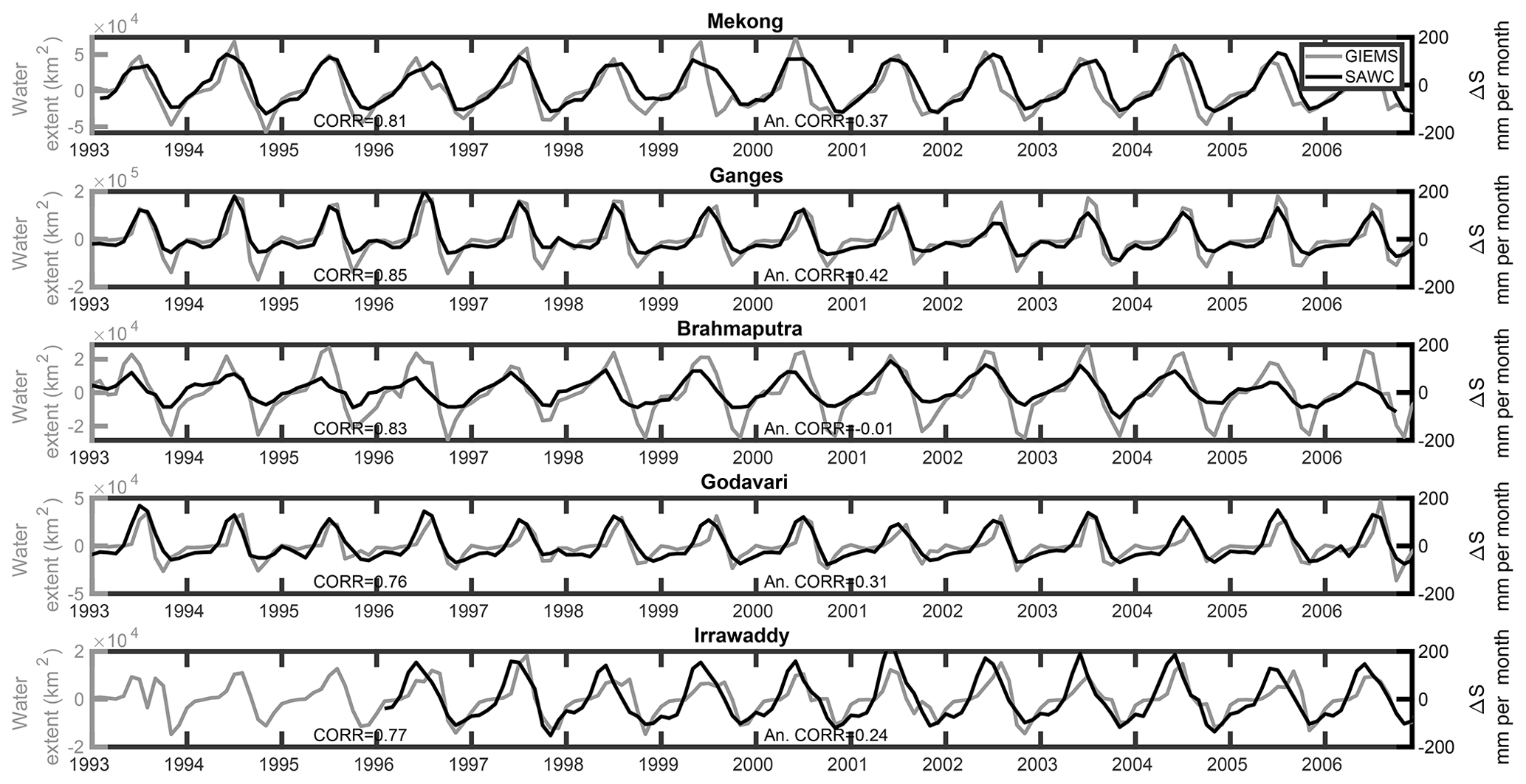
Figure 7 Evaluation of TWSC from the SAWC reconstruction using the GIEMS inundated area from 1993 to 2007 over the figure considered basins. The correlation between them (CORR) is also provided, together with the correlation of the anomalies (An. CORR).

4 Conclusion and perspectives

The total water storage (TWS) as well as its change (TWSC) is a crucial element of the water cycle because of its impact on water management and its role as a tracer of human activity. The first measurement available to monitor it came from the GRACE instrument in 2002. As longer time records are necessary for climate studies, we propose here to use satellite observations for precipitation and evapotranspiration with in situ river discharge measurements to estimate TWSC over the period of 1980–2015. Our approach is based on the water conservation rule over each basin. We performed this task over five major Asian basins because their evolution is related to important questions about water management, climate change and land use changes. Our SAWC reconstruction of TWSC has been evaluated using (1) GRACE observations (over the 2002–2007 period), (2) ISBA model simulations (1980-2015) and (3) surface inundation area (1993–2007). The seasonality and interannual variability of TWS of the SAWC reconstruction appear coherent with these independent sources of information.

The advantages of the proposed methodology are numerous. It is an integration method that gathers all the observations available, from both satellite and in situ measurements. Contrarily to traditional assimilation, this methodology does not use a land or hydrological model, except the water conservation law. It uses the multiplicity of observations to reduce uncertainties for each one of the water cycle components and introduces more hydrological coherency among them. If the river discharge measurement is available, it allows for handling a true anthropized discharge (not an idealized natural one, as provided by models in most cases). However, if this discharge is not available, the methodology cannot be applied; and if important uncertainties on discharge measurements are present, these errors will be propagated to all the other water components.

We foresee many perspectives for this work. First, we would like to extend the TWSC estimation to other basins. This work can be done over large basins (compatible with the GRACE spatial resolution) and where the in situ river discharge measurements are available. Once this is done over a sufficient number of large basins, the optimized databases can be used as a reference to calibrate the satellite estimates at the global scale. This allows for the use of the satellite observations at the global scale and not only over the basins where the integration was performed (Munier and Aires, 2017). River discharges could potentially be estimated over unmonitored basins or over longer time series than the monitoring. Total water storage could also be estimated over monitored basins and over longer times series than the GRACE record (as was done here). When discharge is not monitored, the use of modeled river discharges could be attempted.

Our methodology can also be used to detect incoherencies in our estimations of the water cycle components. For instance, large budget errors could indicate regions where the evapotranspiration is biased (e.g., due to an under- or overestimation of the irrigation, as in the Nile basin). Our approach could detect such problems and propose a bias correction of the specific water component.

Finally, we expect to use a similar methodology over connected subbasins. It is possible to estimate the surface water storage using water extent and topography (Papa et al., 2015), but the horizontal underground transport of water has not been able to be measured so far. The difference of total water storage and surface water storage should help us estimate the ground water storage and characterize its horizontal transport. This would be a major achievement, as this important process of the global water cycle has been largely unknown so far.

Appendix A: Computation of total water storage change (TWSC)

For a given month, TWSC corresponds to the variation of the total water storage (TWS) between the first day of the month and the first day of the following month. As shown in Eq. (1), TWSC equals the sum of inflows into the domain (P) minus outflows out from the domain (E+Q) during the whole month (P, E and Q represent monthly averages). The ISBA land surface model may provide all variables, including TWS, at a daily time step, so that it is possible to compute TWSC as the above-mentioned difference. By construction, the water balance is closed in the ISBA model, and the absolute difference between TWSC and $P-E-Q$ does not exceed 10⁻⁶ mm per month (with a root mean square of 10⁻⁹ mm per month). On the other hand, it is not possible to compute the exact TWSC value with GRACE data, since TWS at the beginning of each month is not available. Instead, GRACE data correspond to monthly averages of TWS anomalies (temporal mean removed). To approximate TWSC, we used the centered difference from Eq. (9). Yet, this approximation introduces important errors compared to the true TWSC value. Figure A1a shows the impact of this approximation with ISBA outputs (where the true TWSC value is represented by $P-E-Q$). To reduce this error, we followed Landerer et al. (2010) by computing $P-E-Q$ using Eq. (6). Figure A1b shows a better match between the approximated $P-E-Q$ and the centered TWSC value. Nevertheless, the reader should keep in mind that both approximations increase final uncertainties by about 5 to 10 mm per month. This error has a quite high frequency and is reduced to less than 1 mm per month when using a 3-year moving average as in Fig. 7.

Figure A1 Comparison between the two estimates of TWSC over the Ganges basin: the closure at any time step in the ISBA model ($P-E-Q$, in blue) and the centered difference of the observed TWS anomalies with GRACE (in red). The difference of the two estimate is also shown (in green). The figure shows the original time series (a) and the seasonal anomalies (b).

Figure A2 Same as Fig. A1, but the closure is now ensured with Eq. (8), following Landerer et al. (2010). This approximation leads to a better match of the two estimates.

Appendix B: Exploration of the 2007 event over Brahmaputra

An extreme inundation occurred in the spring of 2007 over the Brahmaputra basin (Gouweleeuw et al., 2018; Islam et al., 2010; Webster et al., 2010). It is interesting here to analyze how this was handled in the SAWC reconstruction and the ISBA model. Figure B1 compares them for the four water component estimates. The climatological seasons are also represented (dashed lines) for the purpose of comparison. Two basins are illustrated: the Ganges and the Brahmaputra.

In this sample, it can be seen that the model follows classical seasonality for each water component and both basins. In the SAWC reconstruction, the seasonal anomaly is well reproduced for discharge D, which was expected, since this observation was used in the SAWC integration process. This translates into a pronounced anomaly in TWSC. This shows the benefits and the risks associated with the SAWC reconstruction: if the in situ D is reliable, then the SAWC reconstruction will reproduce it well, and the impact on the other components can be important. If D measurements are erroneous, this can introduce considerable noise into the WC analysis.

This relates also to the question of the natural versus real or anthropized discharge D. A hydrological model will generally consider natural rivers. It is difficult to obtain all the necessary information to model true discharge (dam management, pumping for irrigation, etc.). An interesting way to constrain models to follow in situ measurements of the discharge would be to assimilate these measurements into the model (Wang et al., 2018).

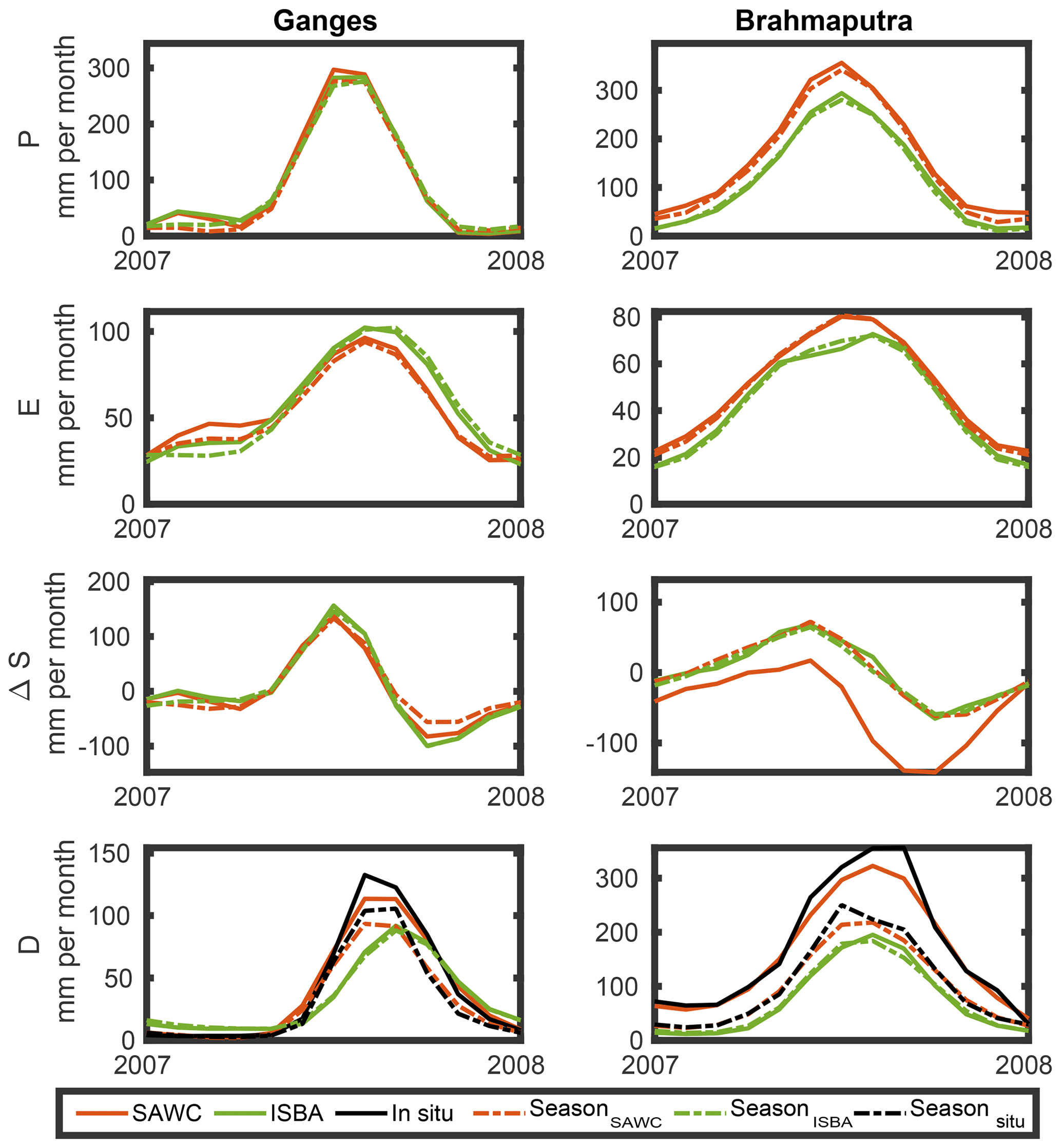
Figure B1 Comparison between the SAWC reconstruction (red) and the ISBA model output (green) estimates for the year 2007 with a large inundation in the Brahmaputra basin for the four water components estimates (in rows) for the Ganges (left panels) and the Brahmaputra (right panels) basins. The climatological season is also represented in dashed lines.