High-resolution fully coupled atmospheric–hydrological modeling: a cross-compartment regional water and energy cycle evaluation

The land surface and the atmospheric boundary layer are closely intertwined with respect to the exchange of water, trace gases, and energy. Nonlinear feedback and scale-dependent mechanisms are obvious by observations and theories. Modeling instead is often narrowed to single compartments of the terrestrial system or bound to traditional viewpoints of definite scientific disciplines. Coupled terrestrial hydrometeorological modeling systems attempt to overcome these limitations to achieve a better integration of the processes relevant for regional climate studies and local-area weather prediction. This study examines the ability of the hydrologically enhanced version of the Weather Research and Forecasting model (WRF-Hydro) to reproduce the regional water cycle by means of a two-way coupled approach and assesses the impact of hydrological coupling with respect to a traditional regional atmospheric model setting. It includes the observation-based calibration of the hydrological model component (offline WRF-Hydro) and a comparison of the classic WRF and the fully coupled WRF-Hydro models both with identically calibrated parameter settings for the land surface model (Noah-Multiparametrization; Noah-MP). The simulations are evaluated based on extensive observations at the Terrestrial Environmental Observatories (TERENO) Pre-Alpine Observatory for the Ammer (600 km²) and Rott (55 km²) river catchments in southern Germany, covering a 5-month period (June–October 2016). The sensitivity of seven land surface parameters is tested using the Latin-Hypercube–One-factor-At-a-Time (LH-OAT) method, and six sensitive parameters are subsequently optimized for six different subcatchments, using the model-independent Parameter Estimation and Uncertainty Analysis software (PEST). The calibration of the offline WRF-Hydro gives Nash–Sutcliffe efficiencies between 0.56 and 0.64 and volumetric efficiencies between 0.46 and 0.81 for the six subcatchments. The comparison of the classic WRF and fully coupled WRF-Hydro models, both using the calibrated parameters from the offline model, shows only tiny alterations for radiation and precipitation but considerable changes for moisture and heat fluxes. By comparison with TERENO Pre-Alpine Observatory measurements, the fully coupled model slightly outperforms the classic WRF model with respect to evapotranspiration, sensible and ground heat flux, the near-surface mixing ratio, temperature, and boundary layer profiles of air temperature. The subcatchment-based water budgets show uniformly directed variations for evapotranspiration, infiltration excess and percolation, whereas soil moisture and precipitation change randomly.

1 Introduction

The intertwined exchange of water and energy fluxes at the land–atmosphere interface determines hydrological processes on a multitude of spatial and temporal scales. Its appropriate formulation and implementation into model systems is a prerequisite for climate and land use change impact investigations. Both terrestrial and atmospheric processes need to be considered. Fully coupled hydrological–atmospheric model systems have recently been developed and comprise the most relevant Earth system components. Comprehensive and concerted evaluation of these coupled modeling systems is required to assess the current limits and potential in Earth system science. This study accordingly focuses on the evaluation of a fully coupled atmospheric–hydrological model across the various compartments of the water and energy cycle.

As shown by Ning et al. (2019), in scientific literature, the topic of coupled hydrological–atmospheric modeling is constantly gaining interest. Several physically based, fully coupled hydrological–atmospheric models have been developed by the scientific community over the past 15 years, addressing nonlinear cross-compartment feedback and fostering a closed representation of regional water and energy cycles (e.g., Shrestha et al., 2014; Butts et al., 2014; Gochis et al., 2016; Soltani et al., 2019). Comprehensive reviews on the history of fully coupled hydrometeorological models and their application can be found in Wagner et al. (2016), Senatore et al. (2015), and Ning et al. (2019). Typically, these models are amalgamations of preexisting subject-specific algorithms of varying complexity, with land surface models being the common thread. Recent applications of fully coupled models show promising results in improving spatial-pattern dynamics and area integrals of regional water budgets. However, the research field is far away from maturity, and many further studies are required.

Using ParFlow coupled with the Community Land Model, Maxwell and Kollet (2008) found that for the US Oklahoma southern Great Plains, groundwater depth governs the sensitivity of regions to variations in temperature and precipitation. Larsen et al. (2016a) reported that by accounting for shallow groundwater in the fully coupled model MIKE SHE, summer evapotranspiration results improved for a study over Kansas, USA. While several studies highlight the importance of lateral hydrological processes for the improved simulation of soil moisture (e.g., Wagner et al., 2016; Larsen et al., 2016a), the sensitivity for land-subsurface–surface–planetary-boundary-layer (PBL) feedback and precipitation generation is less pronounced, especially for the humid regions with strong synoptic forcing (e.g., Butts et al., 2014; Barlage et al., 2015; Arnault et al., 2018; Rummler et al., 2018; Sulis et al., 2018). Coupled modeling studies often focus on single objective variables for validation (like, e.g., discharge, evapotranspiration, or soil moisture) or restrict their analysis to describing only the changes in simulation results without any comparison to observations. Targeting single variables can result in the problem of equifinality, where model realizations are proven skillful for a single aspect yet are possibly wrong for several others. To investigate if a certain model or model configuration can provide improved realism, the limited perspective of single- or few-variable evaluations needs to be abandoned (García-Díez et al., 2015). To overcome the dilemma, fully coupled simulations should be validated and evaluated with respect to as many independent observations as possible. However, the scales of simulations and observations need to match. For catchment-scale coupled hydrometeorological models, most of the global data products (e.g., from satellites) are rather coarse. Regional observatories with integrative measurements of the subsurface-to-boundary-layer fluxes and states provide a sound basis for a holistic evaluation. In the recent past, several efforts have been undertaken to create comprehensive observation sets that allow for subsurface-to-atmosphere integrated studies of water and energy fluxes for small-to-medium-scale river catchments. The most prominent activities for Europe are HOAL (Hydrological Open Air Laboratory; Blöschl et al., 2016), HOBE (the Danish Hydrological Observatory; Jensen and Refsgaard, 2018), LAFO (Land–Atmosphere Feedback Observatory; Spath et al., 2018), and TERENO (Terestrial Environmental Observatories; Zacharias et al., 2011). Although two of them address hydrology in their names, land–atmosphere interaction is a central research item for all of these observatories.

Our study presents a concept to improve the physical realism of regional dynamical hydrometeorological simulations not only by taking into account lateral water redistribution processes on the land surface and their coupled feedback with the planetary boundary layer but also by evaluating the simulated water and energy budgets with comprehensive observations. We calibrate the land surface model that is used in the coupled modeling system based on discharge observations of several subcatchments and thus rely on a variable that integrates the hydrological behavior of the whole upstream area. In a classic local-area modeling study, we could only tune land surface parameters based on station observations, which would be less straightforward with respect to the different scales of simulation and observation. We investigate how well the hydrologically enhanced, fully coupled model mimics observations for different compartments of the hydrological and the associated energy cycle. We evaluate the effect of bidirectional hydrological–atmospheric model coupling with respect to (1) the land surface energy flux partitioning and (2) the different compartments of the hydrological cycle. To that end, we perform uncoupled and fully coupled simulations with the hydrologically enhanced version of the Weather Research and Forecasting modeling system (WRF-Hydro; Gochis et al., 2016) for the Ammer River catchment region, located in southern Bavaria, Germany. We utilize a convection-resolving resolution of 1 km² for the atmospheric part together with a 100 by 100 m hydrological subgrid. For validation, we employ a rich and comprehensive dataset consisting of measurements from the TERENO Pre-Alpine Observatory (Kiese et al., 2018), enhanced by data from the ScaleX field campaign (Wolf et al., 2016), complemented by further local providers.

2 Methods and data

2.1 Study area

The study area covers the two medium-sized river catchments of the Ammer (600 km²) and Rott (55 km²), located in southern Bavaria, Germany (Fig. 1).

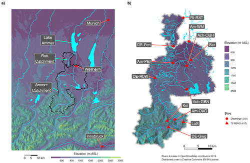
Figure 1 (a) Elevation map for model domain 3 and the location of the Ammer and Rott river catchments. (b) Catchment detail and observation locations. River gauges maintained by the Bavarian Environmental Agency (LfU): Rott-Raisting (Rt-RST), Ammer-Weilheim (Am-WM), Ammer-Peißenberg (Am-PEI), Ammer-Oberammergau (Am-OAG), Ach-Oberhausen (Ach-OBH), and Ach-Obernach (Ach-OBN). TERENO (KIT; Karlsruhe Institute of Technology) Pre-Alpine Observatory sites: Peißenberg-Fendt (DE-Fen), Oberhausen-Berg (Ber), Rottenbuch (DE-RbW), Oberammergau-Kolbensattel (Kol; mountain station), Oberammergau-Laber (LaS; mountain station), and Ettal-Graswang (DE-Gwg). Elevation is derived from ASTER GDEM.

The hydromorphic characteristics of this Alpine front-range region were formed during the last glacial age and predominantly feature Gleysol, Cambisol, and Histosol on top of carbon-based gravel deposits. Elevations range from above 2300 m a.s.l. in the south down to 533 m a.s.l. at the outlet towards Lake Ammer. Land cover is dominated by meadows and forests. The proportion of forests rises from about 20 % in the north to 57 % in the Alpine part of the catchment (Fetzer et al., 1986). Due to the climatic conditions, crops are only of minor importance and are only prevalent in the lower part. Mean annual precipitation exhibits a gradient from 950 mm close to Lake Ammer to more than 2000 mm in the mountains. Mean annual evapotranspiration shows no distinct correlation with elevation and ranges from 300 mm at the sparsely vegetated mountain slopes to 500–600 mm for the rest of the catchment. Mean annual temperature ranges from about 7 to 4 ^∘C between the lower and the upper parts of the catchment.

The study region is part of the German Terrestrial Environmental Observatories program (TERENO; Zacharias et al., 2011), an initiative for the long-term monitoring of climate environmental variables. Our study is bound to the multidisciplinary field experiment and observation campaign ScaleX (Wolf et al., 2016) that took place at the TERENO Pre-Alpine Observatory DE-Fen site (Fig. 1), in the summers of 2015 and 2016.

2.2 Observation data

The study region was selected to cover the Helmholtz Terrestrial Environmental Observatories (TERENO) Pre-Alpine Observatory located in the foothills of the Bavarian Alps of southern Germany. The TERENO Pre-Alpine Observatory features measurements for the range of compartments of the terrestrial hydrometeorological cycle. It has been designed for long-term monitoring of climatological and ecological variables. A detailed description of the concept is available in Kiese et al. (2018). Figure 1b provides an overview of the measurement sites that comprise standard climatological, eddy-covariance, lysimeter, soil moisture, groundwater, and discharge observations.

The observed sensible and latent-heat fluxes presented in this study are determined by means of tower-based eddy-covariance measurements, which are operated on a long-term basis. These installations comprise a CSAT3 sonic anemometer (Campbell Scientific Inc., Logan, UT) at the three main sites (DE-Fen, DE-RbW, and DE-Gwg) of the TERENO Pre-Alpine Observatory and a LI-7500 infrared gas analyzer at DE-Fen and DE-Gwg, while DE-RbW is equipped with a LI-7200 gas analyzer (LI-COR Biosciences Inc., Lincoln, NE, USA). The measurement height of these systems is 3.3 m above ground. High-frequency data from these instruments are recorded digitally on a Campbell CR3000 data logger. The fluxes are computed in the field every day with an industrial PC (personal computer) using the eddy-covariance software TK3 (Mauder and Foken, 2015), including corrections for the misalignment of the anemometer using the double rotation methods (Wilczak et al., 2001), humidity influences on the sonic temperature measurement (Schotanus et al., 1983), spectral losses due to path averaging and sensor separation (Moore, 1986), and density fluctuations (Webb et al., 1980). Automated quality control and uncertainty assessment is applied in accordance with Mauder et al. (2013), which extends the test of Foken and Wichura (1996) by an additional spike test on the high-frequency data, a test on the interdependence of fluxes due to the flux corrections, and a test on the representativeness of the flux footprint (Kormann and Meixner, 2001). Moreover, an energy-balance-closure-adjustment method, which is based on the daily energy balance ratio, is applied to daytime sensible and latent-heat flux data under the condition that the Bowen ratio is preserved (Mauder et al., 2013). Lysimeter data are available for three of the TERENO Pre-Alpine Observatory sites (DE-Fen, DE-RbW, and DE-Gwg). The measurements are separated for representative treatments of extensive and intensive grassland management, in accordance with the local farmer's cutting and fertilizer management (Fu et al., 2017). For this study, data derived from six control lysimeters per site are taken into account (i.e., lysimeters that were excavated at adjacent grassland sites near the experimental site). For each lysimeter, precipitation, evapotranspiration, and groundwater recharge (percolation) is calculated from the variations in total weight and the changes in water volume of the corresponding water tank. Obvious outliers in the weight measurements are removed above thresholds of 1000 and 200 g min⁻¹ for the weight changes of the lysimeters and water tanks, respectively. Furthermore, for separation of signal and noise, the Adaptive Window and Adaptive Threshold filter (AWAT; Peters et al., 2014) is applied to the time series of weight changes of each individual lysimeter and corresponding water tank at a temporal resolution of 1 min. The procedure applied in this study is further described by Fu et al. (2017).

A wireless sensor network at the DE-Fen site, consisting of 55 profiles (5, 20, and 50 cm), provides soil moisture information for a grassland area of roughly 12 ha. The measurement devices are spade-shaped ring oscillator electromagnetic permittivity sensors (Truebner SMT 100; Bogena et al., 2017) with a vertical representativeness of about 3 cm. Additional information on sensor calibration and the conversion of permittivity into volumetric water content is available in Fersch et al. (2018).Within the course of the ScaleX campaign (June–August 2016; Wolf et al., 2016), a scanning microwave radiometer (HATPRO; Humidity and temperature profiler; Rose et al., 2005) provided information on temperature and humidity profiles as well as integrated water vapor and the liquid water path. The instrument measures sky brightness temperature at 14 frequencies. Of these seven are distributed between 22.235 and 31.4 GHz along the wing of the 22.235 water vapor line, and seven are between 51.26 and 58 GHz along the wing of the 60 GHz oxygen absorption complex. Information on atmospheric variables is obtained from the measured brightness temperatures with a retrieval algorithm from the University of Cologne (Löhnert and Crewell, 2003; Löhnert et al., 2009). For the retrieval creation a set of around 14 000 radiosonde profiles, measured at Munich (station at 489 m a.s.l.) between 1990 and 2014, is used. While integrated water vapor has an accuracy of less than 1 kg m⁻² (Pospichal and Crewell, 2007), the vertical resolution of humidity is low, as only two of the seven available water vapor channels are independent (Löhnert et al., 2009). Adding the information from nine elevation scans performed at low angles to the standard zenith observations for the opaque oxygen complex allows for obtaining temperature profiles with a higher spatial resolution and an accuracy of less than 1 K below around 1.5 km (Crewell and Löhnert, 2007). Discharge measurements for the six subcatchments (Ach-OBN, Ach-OBH, Am-OAG, Am-PEI, Am-WM, Rt-RST) evaluated in this study are obtained from the online archive of the Bavarian Environmental Agency (LfU; https://www.gkd.bayern.de, last access: 11 May 2020).

2.3 The WRF-Hydro modeling system

The Weather Research and Forecast modeling system (WRF; Skamarock and Klemp, 2008) is a common, community-developed tool for the simulation of local-area-to-global tropospheric dynamics and their interaction with the land surface. Applications range from short-term regional forecast to long-term continental climate studies with spatial resolutions of a few tens of meters with large-eddy simulations to several kilometers. WRF-Hydro (Gochis et al., 2016) augments WRF with respect to lateral hydrological processes at and below the land surface. It adds a surface storage layer where infiltration excess water is stored and subsequently routed according to the topographic gradient once the retention depth is exceeded. This is different to WRF, where the infiltration excess depicts a sink term. Thus, in WRF-Hydro the surface water can infiltrate gradually, potentially leading to increased soil moisture. Gradient-based routing can also be activated for saturated soil layers, and in case of oversaturation the water will exfiltrate to the surface, where it enters the surface storage body and routing process. WRF-Hydro is connected with the planetary boundary layer in the same way as WRF; the lateral water transport at and below the surface is the crucial difference. Further hydrological processes that are implemented in WRF-Hydro without feedback to the atmosphere are baseflow generation and channel routing. The model has two operation modes: standalone, driven by gridded (pesudo-)observations (one-way coupled), or fully coupled with the dynamic atmospheric model WRF (fully coupled).

The one-way coupled WRF-Hydro system (i.e., separate computations for atmosphere and hydrology without upward feedback) had been successfully applied for short-term forecasting (Yucel et al., 2015) and long-term hindcasting (Li et al., 2017) and was furthermore selected as the core component of the United States National Water Model (NWM; e.g., Cohen et al., 2018; http://water.noaa.gov/about/nwm, last access: 18 July 2019). Fully, two-way coupled applications found reasonable performance for monthly scale discharge simulations for the Sissili (Arnault et al., 2016b) and the Tono (Naabil et al., 2017) basins in western Africa. Reasonable results were also achieved on a daily basis for the Tana River in Kenya (Kerandi et al., 2018). In an ensemble study with the fully coupled WRF-Hydro model, encompassing six catchments in southern Germany, Rummler et al. (2018) found that simulated and observed flow exceeding percentiles on an hourly basis were in good agreement for a 3-month summer period in 2005. Comparison studies with respect to WRF showed slightly improved precipitation skills with WRF-Hydro for the Crati region in southern Italy (Senatore et al., 2015) and for Israel and the eastern Mediterranean (Givati et al., 2016). WRF-Hydro provides a good capability for studying the coupled land–atmospheric boundary system from catchment-to-continental-scale regions. Although many of the recent studies focus on classic precipitation and discharge simulation performance, the ability of the fully coupled model system to improve physical realism for water and energy budgets across compartments becomes increasingly important and is therefore of central interest in this study.

2.4 Model setup and calibration

2.4.1 Modeling chain

The study analyzes the impact of coupling hydrological processes to the regional atmospheric modeling system WRF with respect to water and energy exchange at the land-surface–atmospheric-boundary-layer interface. The lateral flow of infiltration excess, as well as river inflow and routing, are addressed by the WRF-Hydro extension. Several parameters of WRF-Hydro influence the land surface water redistribution and thus the hydrographs and require therefore thorough calibration.

To finally come up with a fully coupled WRF-Hydro setup, several intermediate steps are required that involve different components of the modeling system. As outlined in Fig. 2 we build a modeling chain with the items WRF-Hydro standalone (WRF-H_SA), WRF standalone (WRF_SA), and WRF-Hydro fully coupled (WRF-H_FC). WRF-H_SA refers to the hydrologically extended land surface model that is not coupled to an atmospheric model and gets its driving data from gridded (pseudo-)observations. WRF standalone (WRF_SA) is the classic version of WRF that has no hydrological extension and that is driven by data from a global circulation model. WRF-H_FC extends WRF_SA with the hydrological implementations of WRF-H_SA.

Of the eight driving variables required by WRF-H_SA, only interpolated precipitation is available from observations with adequate coverage. Thus, the remaining input variables (temperature, humidity, wind, and radiation) are taken from a preceding standalone WRF (WRF-ARW 3.7; Advanced Research WRF) simulation.

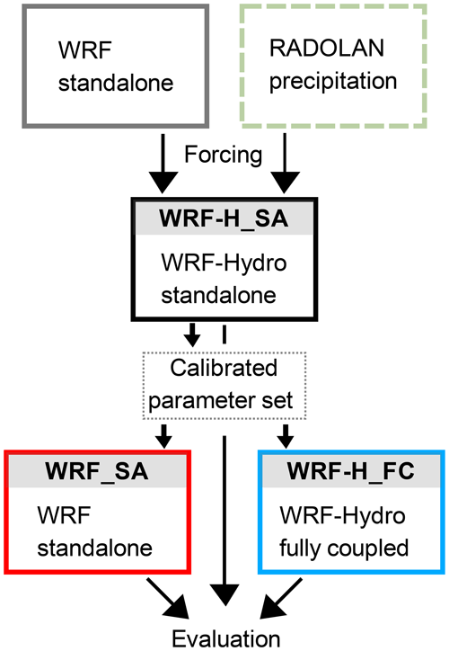
Figure 2 Modeling components and workflow. RADOLAN-RW is an hourly precipitation observation product of the German Weather Service with 1 km² grid resolution.

The modeling chain encompasses the following four steps: (1) a classic standalone WRF run (1 April 2015–31 October 2016) with standard land surface model (LSM) parameters to derive the driving variables required by (2) the standalone WRF-Hydro simulations (WRF-H_SA; 1 April–31 July 2015 and 15 April 2016–31 October 2016) that also ingest hourly gridded observed precipitation (Radar-Online-Aneichung – RADOLAN – of the German weather service – DWD; Bartels et al., 2004; Winterrath et al., 2012), (3) a fully coupled WRF-Hydro simulation (WRF-H_FC; 15 April 2016–31 October 2016) using calibrated parameters from WRF-H_SA, and (4) a rerun of the classic standalone WRF (WRF_SA; 15 April 2016–31 October 2016) with the same parameter set obtained from WRF-H_SA. Finally, this leads to a commensurable set of simulations, coupled vs. uncoupled. Consequently, WRF_SA does not represent an optimized setup of a classic WRF standalone model. Therefore, it is possible that with other parameter combinations for WRF_SA even better performance could be achieved. However, tuning WRF_SA is not easily possible because it does not feature the simulation of discharge and other point observations are sparse and represent different scales. They are thus only suitable for the evaluation of simulation results.

The computational demand was about 0.021 million core hours for the WRF_SA simulations, 0.32 million core hours for the WRF-H_SA calibration runs, and 0.042 million core hours for WRF-H_FC on a 2.3 GHz Intel Haswell system.

2.4.2 Space and time

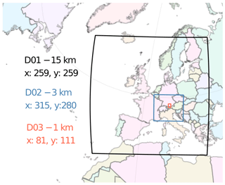
Figure 3 visualizes the domain and nesting configuration for the WRF_SA and WRF-H_FC simulations.

Figure 3 Domain nesting configuration for WRF_SA and WRF-H_FC simulations.

A telescoping configuration with three nests is employed. The horizontal resolutions are 15 by 15, 3 by 3, and 1 by 1 km for domains 1, 2, and 3, respectively. The finest domain extends from the city of Munich in the northeast to the mountain valleys of Inn and Lech in the southwest. For all domains, the number of vertical levels is 51. The model top is defined at 10 hPa. The WRF-H_SA and WRF-H_FC simulations cover the period 15 April to 31 October 2016 including a half month for model spin-up. The starting date corresponds to snow-free conditions for most of domain 3. The spin-up strategy avoids the uncertain simulation of the snow storage dynamics for the winter season. For the surface variables in WRF-Hydro, we consider a 15 d spin-up to be sufficient. The initial (15 April 2016) soil moisture fields for both WRF_SA and WRF-H_FC are taken from the last WRF-H_SA simulation time step (31 October 2016). We assume that this 6-month spin-up period is sufficient to come up with reasonable starting conditions for a commensurable set of simulations. The model runs are performed continuously with none of the variables being reinitialized in between. Lateral surface water flow processes (i.e., overland and channel routing) in WRF-H_SA and WRF-H_FC are computed on a 100 by 100 m grid with the extent being identical to that of domain 3. The integration time steps for the atmospheric part (WRF including the Noah-Multiparametrization – Noah-MP – LSM) are 60, 12, and 4 s for domains 1, 2, and 3, respectively. The hydrological routines are called at hourly intervals.

Thompson et al. (2008)Kain (2004)Sukoriansky et al. (2005)Niu et al. (2011)Iacono et al. (2008)Iacono et al. (2008)

Table 1 Selected WRF_SA and WRF-H_FC model physical schemes. QNSE: quasi-normal scale elimination; RRTMG: Rapid Radiative Transfer Model for General Circulation Models.

^* Only for the outermost domain.

2.4.3 Model physics

The WRF physics parameterization for the selected domains is listed in Table 1. Cumulus parameterization is only activated for the outermost domain 1, while explicit convection is chosen for the finer grids (domains 2 and 3), according to Skamarock et al. (2008).

For uncoupled and coupled simulations, Noah-MP (Niu et al., 2011) is used as the land surface model. For Noah-MP the selected configuration deviates from the default setup as follows: the Community Land Model (CLM) method is selected for stomatal-resistance computation, the Schaake et al. (1996) method is used to determine infiltration and drainage (similar to the classic Noah LSM), the two-stream radiation transfer applied to the vegetated fraction (option 3) is chosen, and the dynamic vegetation option (Dickinson et al., 1998) is enabled.

The static data are adopted from the standard WRF geographic dataset. The land cover for domains 1 and 2 is based on USGS (United States Geological Survey) classification and includes lakes. For the innermost domain the land cover information is based on the CORINE Land Cover (Büttner, 2014) dataset of the European Union, reclassified according to the USGS classes. The elevation data for the 100 m grid are derived from the Advanced Spaceborne Thermal Emission and Reflection Radiometer global digital elevation model (ASTER GDEM, version 2).

Noah-MP provides different options for the computation of groundwater discharge and surface runoff (infiltration excess), but only WRF-Hydro enables the simulation of lateral hydrological processes such as the overland routing of surface runoff and channel (discharge) routing. A short description of the most relevant model details for this study is provided below. Further information about technical features and standard model physics options are given in Gochis et al. (2016), while Sect. 2.4.4 describes the specific improvements made to the original model in order to fit with the specific features of the complex topography of this study area.

In the WRF-Hydro modeling system only subsurface and surface overland flow routing are allowed to directly affect atmosphere dynamics (i.e., only these processes are fully coupled). After every LSM loop, a subgrid disaggregation loop (Gochis and Chen, 2003) is run prior to the routing of saturated subsurface and surface water, in order to achieve the desired spatial refinement (from 1 km to 100 m) for the two-state-variable infiltration excess and soil moisture content. At this stage, linear subgrid weighting factors are assigned for preserving the subgrid soil moisture and infiltration excess spatial variability structures from one model time step to the next. Then, subsurface lateral flow is calculated, using the method suggested by Wigmosta et al. (1994) and Wigmosta and Lettenmaier (1999) within the Distributed Hydrology Soil Vegetation Model (DHSVM). The water table depth is calculated according to the depth of the top of the highest (i.e., nearest to the surface) saturated layer. Finally, overland flow routing also accounts for the possible exfiltration from fully saturated grid cells and is achieved through a fully unsteady, explicit, finite-difference, diffusive-wave approach similar to that of Julien et al. (1995) and Ogden (1997). In this study the steepest descent method is used with a time step of 6 s. After the execution of the routing schemes, the fine-grid values are aggregated back to the native land surface model grid.

Concerning the one-way coupled processes modeled in the WRF-Hydro system (i.e., no feedback with the atmosphere), in this study, the channel flow and baseflow modules are used. Specifically, channel flow routing is performed through an explicit, one-dimensional, variable-time-stepping diffusive-wave formulation. Overland flow discharging into the stream channel occurs when the ponded water depth of specific grid cells, assigned to a predefined stream channel network, exceeds a fixed retention depth. The channel network has a trapezoidal geometry, depending on the Strahler stream order functions. Currently no overbank flow is simulated. Baseflow to the stream network is represented through a simple bucket model which uses an exponential equation to achieve the bucket discharge as a function of a conceptual water depth in the bucket. Several baseflow subbasins (i.e., several conceptual buckets) can be specified within a watershed, but since an empirical equation is used, its parameters need to be estimated for each of the subbasins. The baseflow model is linked to WRF-Hydro through the deep-drainage discharge from the land surface soil column. The estimated baseflow discharged from the bucket model is then combined with the lateral inflow from overland flow and is input directly into the stream network as a part of the stream inflow. The total subbasin baseflow flux to the stream network is equally distributed among all channel pixels within the subbasin.

The reservoir module (retention of channel flow in lakes and reservoirs) is disabled for the simulations of this study because only one gauge (Ach-OBH) would be slightly affected by a 7.66 km² lake (Staffelsee), but the number of calibration parameters and thus calibration runs would considerably increase. Since the lake evaporation is explicitly considered by the Noah-MP land surface model, we do not assume any impact on the land-surface–boundary-layer exchange by this simplification.

2.4.4 Changes with respect to the original WRF-Hydro model

The model, as applied in this study, differs from the version 3 of WRF-Hydro with respect to soil layer representation and model time steps. Large parts of the modeling domain and the considered river catchments exhibit mountainous terrain with steep slopes covered by shallow soil layers. Here, the model's general assumption of 2 m soil thickness (or depth to bedrock) does not hold true, as it may lead to an overestimated retention of infiltrating water. Therefore, in this study, the soil layer definition is changed from a domain uniform to a grid-point-based representation, and soil layer thicknesses are set to the Noah-MP standard (0.1, 0.3, 0.6, and 1 m) distribution for hillslopes below 50 % and to more shallow values (0.05, 0.05, 0.1, and 0.1 m) for all slopes >50 %. The 50 % threshold leads to a realistic discriminability of valley bottoms and hillslopes. In addition, the infiltration (REFKDT) and percolation (SLOPE) parameter implementation is changed from domain-wide uniform values to subcatchment-wise distributed (lumped) values. Another important change is made with respect to the time step configuration of WRF-H_SA and WRF-H_FC simulations. As pointed out in Senatore et al. (2015), differing intervals used for the temporal integration of the Noah LSM lead to inconsistent amounts for the soil water fluxes. The issue is caused by numeric effects when time steps become very small (1 km WRF requires about 4 s) in fully coupled WRF-Hydro simulations with high resolutions. To eliminate the problem and to make all simulations comparable, the hydrology part (subgrid) in WRF-H_FC is only called at an hourly time step, similar to that of WRF-H_SA. In WRF-H_FC the flux variables of domain 3 are therefore cumulated in between the (hourly) calls of the hydrological routines, and on the other hand, the overland routing output (surface head) is returned to domain 3, equally distributed over the LSM time steps (4 s). The subsurface routing option for saturated soil layers is deactivated in this study, as full saturation rarely takes place in the region and because the module would require extending the calibration by two more parameters.

2.4.5 Driving data

Atmospheric boundary conditions for the outer domain of the WRF_SA and the WRF-H_FC simulations are derived from the ERA (ECMWF – European Centre for Medium-Range Weather Forecasts – Reanalysis) Interim reanalysis (Dee et al., 2011) with 0.75^∘ horizontal grid spacing, 37 pressure levels from 1000 to 1 hPa, and 6 h temporal resolution. Forcing data for WRF-H_SA are taken from the standard WRF simulation output for domain 3. The variables comprise near-surface air temperature, humidity, wind, surface pressure, and short- and longwave downward radiation. Since precipitation from WRF simulation is typically biased and dislocated, an observational product of the German weather service (RADOLAN; Bartels et al., 2004; Winterrath et al., 2012) is used for substitution. It combines gauge and rain radar information and is available with an hourly time step and 1 km² resolution.

2.4.6 Calibration

Different approaches for the calibration of the WRF_SA model have been followed in previous works, all of which were based on the comparison of the observed hydrographs. Yucel et al. (2015) adopted a stepwise approach, where the parameters controlling the total water volume were first calibrated (namely, the infiltration factor, REFKDT, and the surface retention depth, RETDEPRT), followed by the parameters controlling the hydrograph shape (namely, the surface roughness, OVROUGHRT, and the channel Manning roughness, MANN). Li et al. (2017), Naabil et al. (2017), Kerandi et al. (2018), and Senatore et al. (2015) followed a similar approach. Specifically, the latter added in the first calibration step the parameter that governs deep drainage (SLOPE) and in the second step the saturated soil lateral conductivity and the bucket outflow exponent (EXPON). Furthermore, to refine calibration they introduced an automated procedure based on the Parameter Estimation and Uncertainty Analysis software (PEST; Doherty, 1994). Arnault et al. (2016b) mainly focused on the REFKDT and, secondarily, on the MANN parameters. Finally, Silver et al. (2017) proposed a satellite-based approach for arid (bare-soil) regions aimed at calibrating topographic slope, saturated hydraulic conductivity, and infiltration parameters, based on physical soil properties and not depending on observed runoff.

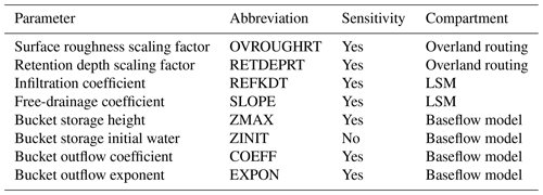
Calibrating a complex hydrological model with a large number of parameters by means of only river discharge can be very problematic, particularly because of the known problem of equifinality (Hornberger and Spear, 1981; Beven, 2006; Beven and Binley, 2014). Several approaches are adopted to reduce or control this problem, particularly challenging for the emerging fully distributed paradigm in hydrology (Beven and Binley, 1992; Beven, 2001; Kelleher et al., 2017), either constraining the parameter set by means of various strategies (e.g., Cervarolo et al., 2010) and/or incorporating different observations than discharge in the calibration process (e.g., Thyer et al., 2004; Stisen et al., 2011; Graeff et al., 2012; Corbari and Mancini, 2014; Larsen et al., 2016b; Soltani et al., 2019). A fully coupled atmospheric–hydrological approach further increases the degrees of freedom of the model, making the issue even more complex. In this study, while the calibration of the hydrological model is performed offline, accounting only for discharges from several cross-river sections, the effect of the resulting parameter set is evaluated considering soil, surface (both in terms of vegetation and hydrology), and atmosphere compartments all together with their reciprocal interactions. Further research will focus on a more thorough analysis of equifinality issues in two-way coupled hydrometeorological models. After several preliminary runs, where the model sensitivity to all the parameters involved in literature calibration procedures is tested, the WRF-H_SA model calibration also follows a two-step approach but in a different sense with respect to Yucel et al. (2015). First, the Latin-Hypercube–One-factor-At-a-Time (LH-OAT; Van Griensven et al., 2006) method is used to determine the sensitivity of a set of eight selected parameters on subbasin river discharge but also to obtain a starting configuration for the automated parameter optimization. The first step includes some iterations to find an optimal threshold value for the delineation of shallow soils on the steep mountain slopes and deeper soils in the plains (see also Sect. 2.4.4). In the next step, seven sensitive parameters are optimized for the six different subbasin outlets (Fig. 1b) using PEST (Doherty, 1994). Table 2 gives an overview of the parameters and their relevance.

Table 2 List of parameters used for WRF-H_SA calibration.

The calibration procedure is adopted for the different subcatchments in cascade, starting from upstream (i.e., parameters are first calibrated for Am-OAG, Ach-OBN, and Rt-RST, then for Am-PEI and Ach-OBH, and, finally, for Am-WM; see Fig. 1b). For LH_OAT the goodness of fit is determined using the volumetric efficiency (VE; Criss and Winston, 2008):

$$\begin{array}{}\text{(1)}& \mathrm{VE}=\mathrm{1}-{\displaystyle \frac{\sum |Q_{\mathrm{obs}}-Q_{\mathrm{sim}}|}{\sum Q_{\mathrm{obs}}}},\end{array}$$

where Q_Obs and Q_sim denote the observed and simulated discharge in m³ s⁻¹ and NSE is the Nash–Sutcliffe efficiency. PEST optimization relies on an objective function given by the sum of squared deviations between model-generated streamflow and observations. Table 3 lists the subcatchment-wise calibrated parameters. The optimum slope gradient for the delineation of shallow and deep soil regions is found to be 50 % (22.5^∘). Accounting for the shallow mountain slopes considerably improves the hydrographs for Am-OAG and Am-PEI, as it increases underestimated peaks and decreases overestimated retention. A comparison of the respective hydrographs and performance measures for calibration and the validation period is shown in Figs. S1 and S2 in the Supplement. Since the study focuses on land–atmosphere exchange, and river routing has no feedback to the LSM, the channel parameters (geometry and Manning roughness coefficient) are not further optimized with respect to peak timing.

The calibration period length of 3.5 months (15 April–31 July 2015, including 14 d of spin-up) is selected as a compromise between the number of model runs (about 2000, which relates to about 0.32 million core hours for WRF-H_SA), which are required during hypercube sampling and PEST optimization, and the available computational resources.

The hydrographs for the calibration and validation periods of the WRF-H_SA runs are presented in Figs. 4 and 5. The final parameter sets and goodness-of-fit measures are listed in Table 3.

Table 3 Calibration parameters for the six subcatchments of the Ammer (Am), Ach, and Rott (Rt), at the gauges Oberammergau (OAG), Peißenberg (PEI), Weilheim (WM), Obernach (OBN), Oberhausen (OBH), and Raisting (RST).

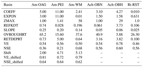
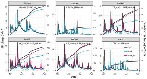
Figure 4 Subcatchment hydrographs for the calibration period (1 May–31 July 2015). Standard WRF-H_SA model output is printed in blue. Shifted (sh) hydrographs are shown in red. Shift amounts are listed in Table 3.

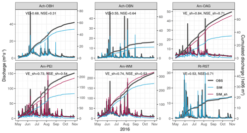
Figure 5 Subcatchment hydrographs for the validation period (1 May–31 October 2016). Standard WRF-H_SA model output is printed in blue. Shifted (sh) hydrographs are shown in red. Shift amounts are listed in Table 3.

For all subcatchments, reasonable configurations could be determined. However, for the three Ammer subcatchments (OAG, PEI, and WM), it was required to add constant baseflow rates of 2, 4.71, and 5.13 m³ s⁻¹ to the simulated hydrographs, respectively. Adding constant baseflow is justified by the fact that due to the glacial processes of the last ice age, large storage bodies, which dip reversely with the surface elevation, were formed in the mountain valleys by overdeepening (Seiler, 1979; Frank, 1979). Further downstream, towards the opening of the valley, where the aquicludes reach towards the surface, springs are abundant. The channel inflow from such long-term storage cannot be realized by WRF-Hydro's conceptual bucket scheme. It would require the implementation of a more sophisticated groundwater model. The underestimation of long-term baseflow by the model has no influence on the land-surface–atmosphere exchange, as there is no interaction of the channel routing with the LSM. The amounts for constant baseflow are derived manually after the PEST parameter optimization so that the recession curves of the simulations agree well with the observations. For the Ach and Rott subcatchments channel, baseflow is related to shallow aquifers with shorter residence times which should be solely captured by the model.

Focusing on the values of the calibrated parameters, it can be observed that the surface infiltration parameter REFKDT, as compared to the standard settings in WRF and Noah-MP (e.g., nominal range of 0.5–5.0, according to Niu, 2011; 0.1–0.4, according to Lahmers et al., 2019), is rather low (therefore allowing lower infiltration) for all subcatchments except Ach-OBH. The associated LSM surface runoff scaling parameter REFDK is globally set to $\mathrm{2}\times {\mathrm{10}}^{-\mathrm{6}}$, as smaller values would have decreased infiltration to even smaller amounts. Also, the percolation parameter SLOPE was mainly reduced as compared to the standard values (0.1–1.0, according to Niu et al., 2011b), meaning that a relatively limited portion of former infiltration excess water is needed to be transferred to the bucket storage to assure good performance for the simulated baseflow. As for the surface overland roughness scaling factors, they generally remarkably increase the standard value of 1.0, contributing to the increase of the hydrograph's lag time and the relative reduction of the peak discharge. The retention depth scaling factors, instead, are much closer to the standard value of 1, varying slowly both the total volumes of the hydrographs and the lag time of the initial response of the catchment to rainfall. The bucket scheme parameters should be evaluated considering their mutual influence on the model exponential equation. In general, the higher the ZMAX value is, the slower the response time of the bucket is, and the higher the COEFF value is, the higher the potential contribution of the bucket model to the total runoff is. From this point of view, the most reactive subcatchment is Am-PEI. In this subcatchment, REFKDT is rather small, and therefore the contribution by the bucket needs to be quicker also because of the rather large subcatchment site. However, this bucket's behavior cannot be appreciated by looking at the hydrographs in Fig. 4 both because in the simulations the values of the bucket storage height are never close to ZMAX and because the resulting discharge in the graph also depends on the contribution of the upstream catchment Am-OAG. During the PEST automated calibration, some parameters hit a boundary limit of the calibration range, which was previously set starting from the results obtained with the LH-OAT method. For example, the optimized ZMAX values hit the lower boundary for the three upstream catchments. In such cases the constraints were relaxed, allowing the parameters to exceed the previous limits, but if negligible or even null improvements were found, we preferred to come back to the previous borders. Finally, it is noteworthy to highlight that, since the study focuses on land–atmosphere exchange and river routing has no feedback to the LSM, the channel parameters (geometry and roughness coefficient) are not further optimized concerning peak timing.

The calibration performed in the spring and summer of 2015 is validated over the period 1 May–31 October 2016 (Fig. 5). The performance statistics for the validation period are comparable to those of the calibration period, and in the cases of Ach-OBN, Am-OAG, and Rt-RST they even improved. For Ach-OBH, as expected due to the disabling of the reservoir option, the buffering effect of the lake cannot be reproduced by the model, thus leading to an overestimation of most of the peak values. However, with respect to the overall discharge in the Ammer catchment, these cutoff peaks are rather small. The performance for Am-WM is lower for both 2015 and 2016, as it aggregates the mismatches of all the upstream subcatchments.

The results of the calibration are in line with other hydrological modeling studies for the Ammer catchment. Ludwig and Mauser (2000) implemented TOPMODEL (Topographical Model; Beven et al., 1984) into a SVAT (soil–vegetation–atmosphere transfer) model framework and yielded an NSE of 0.92 for a 1-year simulation on a daily basis for the gauge Fischen (near Am-WM). Marx (2007) achieved NSE performances of 0.2 (Am-OAG), 0.42 (Am-PEI), 0.75 (Am-WM), 0.68 (Ach-OBN), and 0.18 (Ach-OBH), using WaSiM-ETH (Water Balance Simulation Model; Schulla and Jasper, 2007) for the year 2001. Rummler et al. (2018) obtained an NSE of 0.91 with the WRF-Hydro standalone model for Am-PEI, for a 3-month simulation of a major flood event in 2005.

The commonly favored lumped calibration of WRF-Hydro seems to be rather limited, concerning the transferability of parameter sets among subcatchments and with respect to the numerical efficiency for automated calibration. Especially for complex terrain, e.g., as presented by this study, the distribution of discharge gauges does not agree with landscape units. Therefore, the lumped-parameter sets have to unify quite diverse subcatchment conditions which may lead to unrealistic spatial representations of the physical properties they represent. Thus, for further studies, it is recommended to find parameter sets that are bound to landscape characteristics, such as relief, land cover type, and soil features (e.g., Hundecha and Bárdossy, 2004; Samaniego et al., 2010; Rakovec et al., 2016; Silver et al., 2017), which also contribute to reduce the equifinality problem (Kelleher et al., 2017).

3 Results and discussion

The following section evaluates and discusses the simulations of the standalone WRF (WRF_SA) and the fully coupled WRF-Hydro (WRF-H_FC) models. In the first part, based on the TERENO Pre-Alpine Observatory stations, the energy fluxes at the land–atmosphere boundary are analyzed, in particular radiation, heat fluxes, near-surface air temperature, evapotranspiration, and soil moisture. The second part compares modeled and observed atmospheric-boundary-layer profiles for the DE-Fen site. The third part deals with the subcatchment-aggregated water budgets and looks at the differences in the temporal evolution of simulated soil moisture patterns.

3.1 Model evaluation for TERENO Pre-Alpine Observatory stations

3.1.1 Radiation

The evaluation of WRF_SA and WRF-H_FC simulations with measurements from the TERENO Pre-Alpine Observatory focuses on the radiation input, its partitioning into water, and energy fluxes at the land surface and on the near-surface atmospheric and subsurface states. Figure 6 shows the mean diurnal cycles of simulated and observed downward surface shortwave radiation for three TERENO Pre-Alpine Observatory sites for the period June to October 2016.

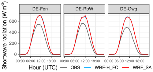
Figure 6 Mean diurnal cycles of simulated and observed downward surface shortwave radiation for June to October 2016.

For all locations, the simulations overestimate radiation from sunrise to sunset with similar magnitude. While correlations for the hourly values are high (r² for DE-Fen of 0.76, DE-RbW of 0.73, and DE-Gwg of 0.66), the mean errors (MEs in W m⁻² for DE-Fen of 61, DE-RbW of 57, and DE-Gwg of 78) reveal considerable bias. Also the mean absolute errors show substantial scatter (MAEs in W m⁻² for DE-Fen of 89, DE-RbW of 91, and DE-Gwg of 107). The overestimation of summer shortwave radiation for central Europe with WRF has also been documented by other studies and is usually related to underestimated cloud cover, especially in the mid troposphere, where convection is active (García-Díez et al., 2015; Katragkou et al., 2015). The increased bias for DE-Gwg could be related to local shading due to topography in this narrow Alpine valley and because of higher convective activity in this mountain region. The comparison of the WRF_SA and WRF-H_FC simulations does not yield considerable differences.

The results for downward longwave radiation are given in Fig. 7.

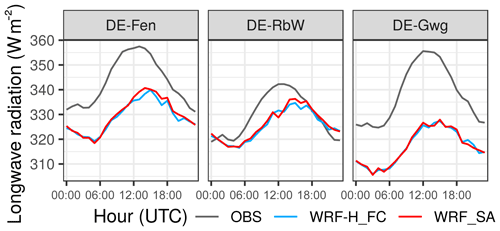
Figure 7 Mean diurnal cycles of simulated and observed downward longwave radiation for June to October 2016.

The negative biases for the different locations (ME in W m⁻² for DE-Fen of −14, DE-RbW of −4, and DE-Gwg of −21) correspond with the above-suggested cloud cover underestimation. With −1 % to −6 %, the relative deviations are rather small. Again, the differences between the standalone and coupled models are nominal. A similar overestimation is obtained for total absorbed shortwave radiation (Table S1 in the Supplement). Thus, for the TERENO Pre-Alpine Observatory locations it can be stated that shortwave radiation input to the land surface is overestimated by 33 % to 56 % by both the standalone and coupled models.

3.1.2 Heat fluxes and evapotranspiration

The diurnal cycles of latent- and sensible-heat fluxes are presented in Figs. 8 and 9 for three different grassland sites. Converted evapotranspiration rates are plotted alongside in Fig. 8. The analysis is split by month from June to October 2016 to provide insight about the temporal variations. The observations comprise data from flux towers and lysimeters. Their spread can be seen as a measure of uncertainty. The measurements for the flux tower at DE-RbW are missing from 25 September to the end of October.

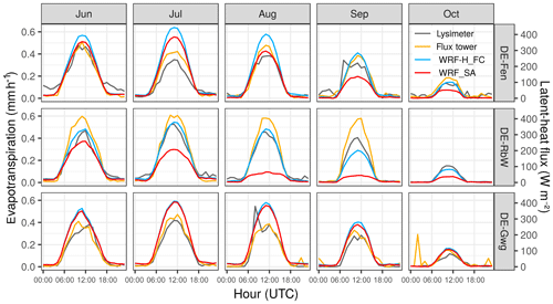
Figure 8 Mean diurnal cycles of simulated and observed latent-heat flux and evapotranspiration for the months June to October 2016 at different TERENO Pre-Alpine Observatory sites.

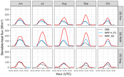
Figure 9 Mean diurnal cycles of simulated and observed sensible-heat flux for the months June to October 2016 at different TERENO Pre-Alpine Observatory sites.

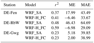
The coupled WRF-H_FC simulation exhibits increased latent- and decreased sensible-heat fluxes for the DE-Fen and DE-RbW sites, whereas WRF_SA and WRF-H_FC are very similar for the Alpine valley location (DE-Gwg). In the case of sensible-heat flux, the hydrologically enhanced model (WRF-H_FC) outperforms or is equal to the standalone simulation (WRF_SA). For latent heat and evapotranspiration, the mean diurnal fluxes are overestimated for DE-Fen for June to August by either both models or the coupled run. A constant positive bias is also found for DE-Gwg (except for October). Tables 4 and 6 list the performance measures for observations of latent and sensible heat vs. the flux tower for the period June to October 2016; Table 5 provides the measures for data of evapotranspiration vs. the lysimeter.

Table 4 Performance measures for latent-heat flux (W m⁻²) with simulations vs. flux-tower observations for June to October 2016.

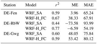
Table 5 Performance measures for evapotranspiration (mm h⁻¹) with simulations vs. lysimeter observations for June to October 2016.

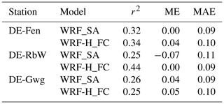
For latent heat and likewise evaporation, correlation improves considerably for DE-Fen and DE-RbW with the coupled model, but ME and MAE deteriorate for DE-Fen and DE-Gwg. An overall improvement for WRF-H_FC with respect to the observations is only obtained for DE-RbW. In general, the simulations are in better agreement with the flux-tower data than with those of the lysimeters. This could be related to the difference in spatial support of the measurements. For sensible heat, the coupled run yields improved performance for DE-Fen and DE-RbW and is also in good agreement with the observations at DE-Gwg.

Table 6 Performance measures for sensible-heat flux (W m⁻²) with simulations vs. observations for June to October 2016.

Ground heat flux (Fig. S3) is overestimated by the models from about 2 h after sunrise until noon. From afternoon till dawn, both simulations overestimate the upward (land-to-atmosphere) radiative flux. WRF_SA and WRF-H_FC differ slightly for ground heat fluxes, with WRF-H_FC showing slightly increased performance with respect to the observations (Table S2).

3.1.3 Near-surface temperature and humidity

The diurnal course of 2 m air temperature (Fig. S4) is similar for uncoupled and coupled model for June and October for all stations. The mountain peak stations (Kol and LaS) and the alpine valley station (DE-Gwg) are hardly sensitive to coupling. Prominent deviations between WRF_SA and WRF-H_FC occur for July to September at the foreland stations (DE-Fen, DE-RbW, and Ber). Here, the coupled simulations between 06:00 and 18:00 UTC agree better with the observations. Nighttime values are generally overestimated by both models, and coupling does not have an influence. The mean errors improve between 0.34 and 0.6 K for the foreland and between 0.11 and 0.25 K for the mountain stations, whereas correlation remains identical. A slight improvement with coupling is also obtained for the MAE values (Table S3).

Figure 10 provides the monthly diurnal cycles for the 2 m mixing ratio. The model comparison reveals higher values for the coupled model run, especially during sunshine hours (06:00–18:00 UTC). Also prominent is a peak in 2 m moisture around 17:00 UTC for both models that is not as pronounced in the observations.

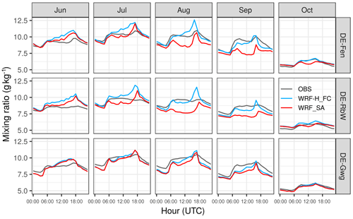
Figure 10 Mean diurnal cycles of simulated and observed 2 m mixing ratio for the months June to October 2016 at different TERENO Pre-Alpine Observatory sites.

For July to August, the coupled simulation resembles the observations better for the morning rise in moisture concentration, but towards the afternoon, the constant rise exceeds the measurements. According to the performance measures in Table 7, the correlation increases considerably with the WRF-H_FC configuration for the DE-Fen and DE-RbW sites. Also ME and MAE are reduced. For DE-Gwg the findings are similar; however the magnitudes are lower.

Altogether, it can be stated that the hydrologically enhanced setup (i.e., WRF-H_FC) leads to an improved representation of 2 m temperature and mixing ratio.

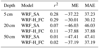
3.1.4 Soil moisture

Observed and simulated soil moisture for the DE-Fen site are presented in Fig. 11.

Table 7 Performance measures for 2 m mixing ratio (g kg⁻¹) with simulations vs. observations for June to October 2016.

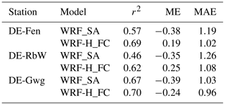
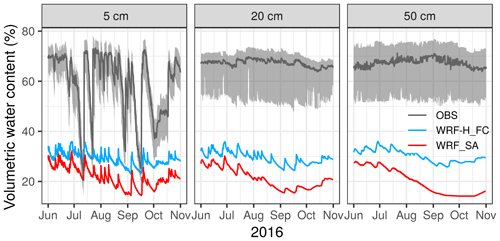
Figure 11 Volumetric water content at the DE-Fen site for three different depths. Gray ribbon: range between first and third quartile of SoilNet observations; gray line: median of SoilNet observations

The gray ribbons depict the 25th to the 75th percentiles of a wireless soil moisture sensor network that consists of 55 profiles with measurements at 5, 20, and 50 cm depth (SoilNet; further details are available at Kiese et al., 2018; Fersch et al., 2018). Obviously, simulations and observation show a considerable offset, and also the temporal variations are much smoother for the model. The discrepancies in the soil moisture time series are largely attributable to the difference in saturation water content. The LSM assumes loam for the DE-Fen site (and almost for the entire area of domain 3) with a maximum volumetric soil moisture content of 44 %, whereas in reality the region consists of sandy-to-silty loams and also peaty areas where the maximum soil moisture ranges between 50 % and 80 %. With WRF-H_FC the soil moisture values are about 8 %–10 % higher than with WRF_SA. Also the decline differs between the two with WRF_SA leading to a much dryer scenario for the summer months. That is where WRF-H_FC-simulated latent-heat flux and evapotranspiration largely outperform. Altogether, for DE-Fen, the decline predicted by WRF-H_FC seems more realistic with respect to the observations. This is also confirmed by the mostly improved statistical measures (Table 8). The representation of soil moisture in LSMs is a general challenge. Soil parameters and water content are often tuned to unrealistic values for the sake of obtaining a good matching of the surface exchange fluxes with observations (Koster et al., 2009). The recent publications of global and continental high-resolution soil hydraulic datasets (like, e.g., Hengl et al., 2017; Tóth et al., 2017) are helpful to improve and unify soil moisture representations in those models. However, these datasets, with their underlying water retention models (e.g., Van Genuchten, 1980), are not supported by the Noah LSMs, and an implementation would be out of the scope of this study.

Table 8 Soil moisture performance measures (vol. %) for DE-Fen for June–October 2016.

Figure 12 Performance evaluation of vertical atmospheric profiles of air temperature (upper panel) and absolute humidity (lower panel) for the DE-Fen site for 1 June–31 July 2016. r²: coefficient of determination; ME: mean error; MAE: mean absolute error.

3.2 Boundary layer profiles during ScaleX campaign 2016

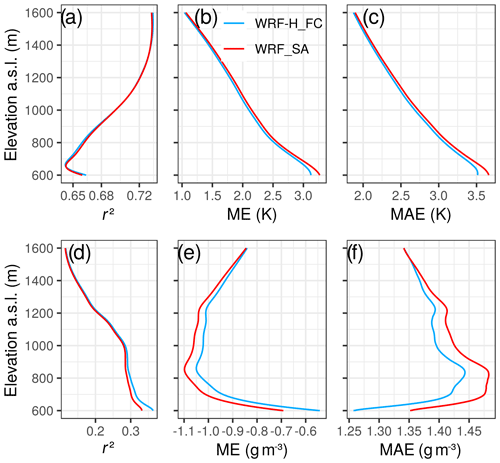
Figure 12 shows the spline-interpolated vertical profiles of the performance measures for the WRF_SA and WRF-H_FC simulations and the HATPRO observations for the planetary boundary layer. The measurements represent hourly subsampled time series from 1 June–31 July 2016 for air temperature (Fig. 12a, b, c) and absolute humidity (Fig. 12d, e, f). For temperature, the differences between HATPRO and the models are generally much larger than the HATPRO accuracy. For humidity, the mean deviation lies within the accuracy of the measurement. It can be followed that both models overestimate temperature and probably have a tendency to underestimate absolute humidity. As compared to WRF_SA, WRF-H_FC shows reduced deviations for both variables.

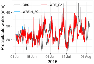
The increase in correlation and the decrease of errors with height is only visible for temperature. The comparison between WRF_SA and WRF-H_FC reveals some modifications for the near-surface region, where the fully coupled model gives a slightly improved skill. For absolute humidity, the lower parts of the profiles are in better agreement with the observations. With 0.15 to 0.35, the coefficients of determination are small as compared to 0.64 to 0.73 for temperature. The WRF-H_FC run outperforms WRF_SA especially for the lower 400 m of the profile. The time series of simulated and observed integrated water vapor for the DE-Fen site are shown in Fig. 13.

Figure 13 Simulated and observed precipitable water for the DE-Fen site for 1 June–31 July 2016.

The temporal evolution is reasonably covered, with a few larger mismatches at the end of June and the end of July. The intermodel differences are very small. Both simulations show nearly identical performance with r²=0.42, ME = −0.21 and −0.19 mm, and MAE = 3.34 and 3.34 mm for WRF_SA and WRF-H_FC, respectively. The results for integrated water vapor and humidity profiles indicate that the coupling mainly affects the atmospheric boundary layer, as differences in the correlation and errors between both simulations are restricted to the lower heights. Moreover, the domain area seems too small for internal moisture recycling and additional precipitation generation to take place. Most of the surplus in humidity is probably transported beyond the domain boundary. If the coupled simulation was extended to a larger area, e.g., Europe, impact above the boundary layer would be expected, at least for periods of weak synoptic forcing (Arnault et al., 2018).

3.3 Water budgets

3.3.1 Analysis for subbasin integrated water balances and discharge

Figure 14 visualizes the monthly water budgets for the six different subcatchments for WRF_SA, WRF-H_FC, and WRF-H_SA (standalone WRF-Hydro) simulations, according to the water balance equation $P=E+R_{\mathrm{SF}}+R_{\mathrm{UG}}+\mathrm{\Delta }{S}_{\mathrm{soil}}$, where P is precipitation, E is evapotranspiration, R_SF and R_UG are surface and subsurface runoff, and ΔS_soil is soil storage variation.

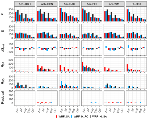
Figure 14 Monthly water budgets in millimeters for subcatchments of the Ach, Ammer (Am), and Rott (Rt). P: precipitation; E: evapotranspiration; ΔS_soil: soil water storage change; R_sf: surface runoff; R_UG: underground runoff (groundwater recharge). WRF_SA: standalone WRF model; WRF-H_FC: fully coupled WRF-Hydro model; WRF-H_SA: observation-driven WRF-Hydro standalone model.

Deviations in subcatchment-aggregated precipitation are small for WRF_SA and WRF-H_FC. P in WRF-H_SA, which originates from the gridded observation product (RADOLAN), differs for most of the months and regions. WRF_SA and WRF-H_FC overestimate P for the mountainous regions (Am-OAG and Am-PEI) for May and June. For the other subcatchments the months of June to August are mainly underestimated. September and October are well resembled for Rt-RST. For the others, October sums are overestimated. For evapotranspiration E an increasing tendency can be seen from WRF_SA via WRF-H_FC to WRF-H_SA. An underestimated P in WRF_SA and WRF-H_FC results in a decreased E. For the Am-OAG subcatchment, the overestimation in P is transferred to surface and subsurface runoff. This is likely because of the soil moisture in the mountain region is generally higher and E is rather energy limited and therefore cannot increase considerably. Moreover, slopes are steeper, and soil thickness is reduced so that percolation takes place quickly. The variation in soil volumetric water content is irregular among models and for the different months. This indicates a nonlinear feedback for the land–atmosphere interaction. Soil infiltration generally increases with the hydrologically enhanced models; however, the amounts for WRF-H_FC and WRF-H_SA vary according to P. Storage depletion (negative values) does not exhibit any tendency among the different models. Surface runoff (infiltration excess) with WRF_SA is 50 % (for some of the subcatchments more than 100 %) higher than with WRF-H_FC and WRF-H_SA. Conversely, groundwater recharge (soil drainage) increases for the hydrologically enhanced models. Again, differences between WRF-H_FC and WRF-H_SA are due to the individual precipitation amounts. On a monthly scale, changes of the canopy water storage compensate (not shown). The water budget residuals, caused by the subgrid aggregation and disaggregation and by other numerical artifacts, can reach up to 31 mm for WRF-H_FC at Rt-RST in September, but in the mean they are 5.6 mm. Altogether, the coupling with hydrology leads to increased infiltration and slightly increased E but almost no changes in P. A reason for this could be that the distance of the displacement between precipitation generation and falling locations is generally much larger than the one covered by the domain boundaries in this study (Arnault et al., 2016a; Wei et al., 2015).

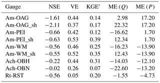
Table 9 lists the performance measures for the discharge simulated with the fully coupled model (hydrographs available in the Fig. S3) with baseflow-shifted simulations (compare Table 3, WRF-H_SA calibration) denoted by sh. Nash–Sutcliffe efficiency (NSE) values are poor for all stations; Kling–Gupta efficiency (KGE'; Kling et al., 2012) values lie between 0.07 and 0.39 with a general performance gain for the baseflow-shifted time series. For all subcatchments except Am-OAG, negative MEs are observed, with values ranging from −22.6 to 2.98 mm per month. For the three Ammer gauges (OAG, PEI, and WM), adding the baseflow shifting leads to an improved baseline of the hydrographs and volumetric efficiency but also to considerable overestimation of the cumulated sums. If the non-shifted MEs for Q are compared with those of P, it turns out that for some of the subcatchments (Am-WM, Ach-OBH, and Rt-RST), the deviations are of a similar amount as precipitation bias. The poor performance of the fully coupled simulation to predict hourly discharge can be clearly mapped to the model's difficulty in reproducing the timing and positioning of precipitation.

Table 9 Discharge performance measures for subcatchment gauges modeled with the fully coupled WRF-H_FC model for June to October 2016. The gauges marked with sh denote the shifted discharge simulation results as applied in the WRF-H_SA calibration (Table 3). Mean errors (MEs) for Q (discharge) and P (precipitation) are given in millimeters per month.

Figure 15 Time series of root mean square deviations between empirical variograms of WRF_SA and WRF-H_FC for soil moisture layers 1 to 4, based on 10 equidistant lags (1 to 10 km).

3.3.2 Spatial variations of simulated soil moisture patterns

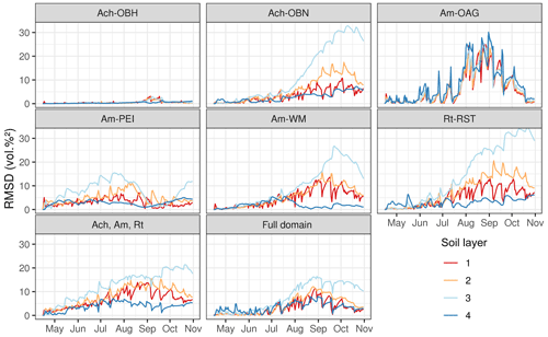
Figure 15 shows the time series of root mean square deviations (RMSDs) of the spatial variograms for the WRF_SA and WRF-H_FC simulations subdivided by the four soil layers in the model. The variograms were computed using 10 equidistant lags of 1 km from 1 to 10 km. The RMSDs were computed for the six different subcatchments; for the Ach, Ammer, and Rott catchments; and for the full domain. For the calculation, the subregions were masked so that the adjacent areas and lakes did not impact the results. The analysis reveals that the structural differences between the two models have their maximum in late summer and fall. Surprisingly, layer 3 gives the strongest variations in spatial patterns. The changes for layers 1 and 2 are not so pronounced. The cause for this might be that the thinner top layers are strongly influenced by precipitation and infiltration processes, and thus the spatial patterns are shaped accordingly. Due to its larger thickness, layer 3 reacts more sluggishly. Thus deviations are more persistent. Layer 4 is even thicker but shows only slight variations over time. It is likely that the free-drainage boundary condition has a regulatory effect here. Also the withdrawal of water for plant transpiration is partly reduced, as only forest land cover classes have roots in this layer per definition. Am-OAG depicts a special case as soil layers are considerably thinner for the steep mountain slopes (see Sect. 2.4.4). Thus, response times are short, and the routing of infiltration excess water is quickly propagated through all layers. The variability for the united Ach, Ammer, and Rott catchments is less pronounced than seen for the smaller entities, but still the maximums are from late summer to fall, and layer 3 is affected most.

4 Summary, conclusive remarks, and perspectives

The calibration of water-related land surface parameters is hardly used for local-area and regional climate model applications. The incorporation of water budgets in the model optimization provides an additional means to evaluate with independent observations. Such a concept requires a coupled atmospheric–hydrological approach that relates the land-surface-to-planetary-boundary-layer exchange of energy and water with the spatial-redistribution processes of water, thus enabling the closure of the regional water balance and complex feedback processes at the land–atmosphere boundary.

This study examines the skills of a classic and a hydrologically enhanced and fully coupled setup of the Weather Research and Forecasting model (WRF and WRF-Hydro) to reproduce the land–atmosphere exchange of energy and water as well as the water budgets of the Ammer and Rott watersheds in southern Germany, for a 6-month period in 2016. The evaluation is based on comprehensive measurements available from the TERENO Pre-Alpine Observatory and further third-party data suppliers such as the Bavarian Environmental Agency.

A standalone version of the WRF-Hydro model (without the atmospheric part), driven by WRF-simulated meteorological variables and observed precipitation (RADOLAN) was calibrated for six different subcatchments, and the resulting parameters were subsequently used for a standalone WRF and a fully coupled WRF-Hydro simulation both being identical with respect to initialization, parameters, forcing, and binary code. The calibration of the standalone WRF-Hydro model (WRF-H_SA) based on observed precipitation yielded reasonable results in terms of Nash–Sutcliffe and volumetric efficiencies. For the Ammer subcatchments (OAG, PEI, and WM), due to long-term hydrogeological storage processes that cannot be reproduced by WRF-Hydro, it was required to correct the negative biases of the baseflow. The volumetric efficiency measure was an important indicator for further optimizing the parameters when Nash–Sutcliffe and Kling–Gupta efficiencies already converged.

For the validation period (1 May–31 October 2016), the skill measures could largely outperform those of the calibration period. However, some structural deficiencies like the underestimated baseflow in the mountainous parts or negative bias remain. It is concluded that some of the processes in the catchment cannot be depicted because of the model physics or the lumped-parameter estimation approach. Altogether, the subcatchment-by-subcatchment calibration is a very time-consuming effort, even if done in a semi-parallel way, which is in our opinion not applicable for larger study regions such as on the national or continental level. A solution might be to switch to a land-characteristics-based universal method or to use a multiscale parameter regionalization method as, for example, described in Mizukami et al. (2017). For the fully coupled WRF-Hydro run (WRF-H_FC), to obtain commensurable quantities for the evaluation, instead of calling the hydrological subgrid functions at every WRF model time step (4 s), an hourly time step identical to that of the WRF-H_SA model was required. The strategy was selected to avoid numerical truncation effects in the overland routing routines that happen when time steps are in the order of a few seconds and the spatial resolution is about 100 m or below (see also Sect. 2.4.4). The most prominent impact of the enabled lateral routing, on WRF-H_FC vs. WRF_SA, is a general increase in soil moisture values due to lateral water transport at the land surface, which in turn leads to increased evapotranspiration for the summer months. Compared to the observations, the coupled simulation performs better for most of the months, and this finding holds also for the fluxes of sensible and ground heat. Solely for the mountainous site (DE-Gwg), both models show almost identical results which we attribute to generally higher soil moisture in that region and also to the reduced soil water storage capacity that comes with the decreased layer thicknesses defined for the slopy regions. In addition to the fluxes, also the near-surface states for air temperature and mixing ratio are better met with the fully coupled model. The comparison with observed boundary layer temperature and humidity profiles at the DE-Fen site also yields a higher rank for the WRF-H_FC simulation. WRF_SA yields much dryer soil moisture conditions, and in particular from July to September it cannot maintain the evapotranspiration that is seen from the observations. However, when compared with the SoilNet data at the DE-Fen TERENO Pre-Alpine Observatory site, a considerable mismatch remains ascribable to the discrepancy of the soil maps used in the model and real world conditions.

The State Soil Geographic–Food and Agriculture Organization (STATSGO–FAO) data assume silty loam for almost the entire area of domain 3. This does not even rudimentarily reflect the complexity of the northern limestone Alps and foothills (compare to Hofmann et al., 2009, for the Halbammer subcatchment of the Ammer), in particular with the high resolutions of 1 km and 100 m of the atmospheric and hydrological model sections. The incorporation of high-resolution continental or global soil maps like, e.g., recently made available by Hengl et al. (2017) and Tóth et al. (2017) could lead to further improvement here. The intermodel deviations for precipitation are marginal. The increased latent-heat flux of the fully coupled model does not strongly impact the precipitation generation for the study domain. It is rather assumed that the surplus in atmospheric moisture is actually being transported beyond the lateral boundaries. Thus, to see an impact of the model coupling on precipitation patterns, the domain size should be sufficiently enlarged. It should be noted that, however, the impact of the lateral water transport modeling on average precipitation amounts may be much less important than, e.g., the selection of the PBL scheme (Arnault et al., 2018). The findings are also corroborated by water-vapor-tagging studies that conclude that regional precipitation recycling is largest during weak synoptic forcing and that variations on larger scales are rather small (Wei et al., 2015; Arnault et al., 2019). Nevertheless, for larger regions the impact may be considerable. Short- and longwave radiation do not change much with the different model configurations. As for precipitation, the land–atmosphere feedback of moisture by LSM–hydrological coupling has no noticeable impact on the cloud generation processes, thus leaving the biases unaffected.

The analysis of the subcatchment water budgets reveals a clear connection between the biases of precipitation, soil infiltration, evapotranspiration, and discharge. The other terms of the water balance equation, soil water storage variation, and percolation do not show distinct trends between standard and coupled simulations, which could be related to the inter-subcatchment variations of the infiltration and percolation parameters.

Using the calibrated parameters of WRF-H_SA in WRF-H_FC is required from a physical perspective. If deviation patterns reoccurred, a recalibration of WRF-H_FC could lead to improved discharge simulations, however at the risk of deteriorating the other water budgets.

In contrast to the uncoupled WRF model, fully coupled simulations with an observation-calibrated hydrologically enhanced LSM show partly improved skill for land–atmosphere exchange variables, although the physical realism of the hydrological extension as well as for the spatial patterns of static data is still limited. Additional efforts are required to increase this physical realism, which should further improve the skill of the overall system. Nevertheless, including hydrological processes provides an additional way to calibrate and evaluate the simulations by also taking the regional water balance and budgets into account, provided that comprehensive observations are available.

The evaluation included the standalone WRF (WRF_SA) and the fully coupled (WRF-H_FC) models that share identical parameter sets and initial and boundary conditions for a commensurable set of simulations. It is of course possible that other parameter combinations for WRF_SA could lead to similar or even better performance as with WRF-H_FC. For example, the dryer soils could be alleviated by increasing the value of the infiltration parameter REFKDT which in turn would increase evapotranspiration and decrease sensible heat. WRF_SA could be parameterized with a domain-wide setting with respect to point observations (e.g., latent-heat fluxes or soil moisture measurements), which however do not guarantee the same accuracy in the remaining area, and the effects of the intermediate surface water storage and lateral flow that are particularly important for strong precipitation events would not be considered. In contrast, the hydrological model allows for taking into account representative features of a wide (catchment) area, summarized in the discharge variable.

The combined approach offers the potential to improve future Earth system modeling, as also pointed out by Clark et al. (2015). To experience the full momentousness of coupled atmospheric–hydrological modeling, future studies should be extended to larger regions to cover the scales of atmospheric recycling processes. Also the descriptions of the hydrological processes in the models should be further refined as computational capabilities increase and as more and more detailed data products become available.