the Creative Commons Attribution 4.0 License.
the Creative Commons Attribution 4.0 License.
 | 30 Apr 2020
Time-lapse cross-hole electrical resistivity tomography (CHERT) for monitoring seawater intrusion dynamics in a Mediterranean aquifer
Andrea Palacios
Juan José Ledo
Niklas Linde
Linda Luquot
Fabian Bellmunt
Albert Folch
Alex Marcuello
Pilar Queralt
Philippe A. Pezard
Laura Martínez
Laura del Val
David Bosch
Jesús Carrera
Surface electrical resistivity tomography (ERT) is a widely used tool to study seawater intrusion (SWI). It is noninvasive and offers a high spatial coverage at a low cost, but its imaging capabilities are strongly affected by decreasing resolution with depth. We conjecture that the use of CHERT (cross-hole ERT) can partly overcome these resolution limitations since the electrodes are placed at depth, which implies that the model resolution does not decrease at the depths of interest. The objective of this study is to test the CHERT for imaging the SWI and monitoring its dynamics at the Argentona site, a well-instrumented field site of a coastal alluvial aquifer located 40 km NE of Barcelona. To do so, we installed permanent electrodes around boreholes attached to the PVC pipes to perform time-lapse monitoring of the SWI on a transect perpendicular to the coastline. After 2 years of monitoring, we observe variability of SWI at different timescales: (1) natural seasonal variations and aquifer salinization that we attribute to long-term drought and (2) short-term fluctuations due to sea storms or flooding in the nearby stream during heavy rain events. The spatial imaging of bulk electrical conductivity allows us to explain non-monotonic salinity profiles in open boreholes (step-wise profiles really reflect the presence of freshwater at depth). By comparing CHERT results with traditional in situ measurements such as electrical conductivity of water samples and bulk electrical conductivity from induction logs, we conclude that CHERT is a reliable and cost-effective imaging tool for monitoring SWI dynamics.
- Article
(11407 KB) - Full-text XML
- BibTeX
- EndNote


Seawater intrusion (SWI) increasingly affects the ever-growing populations near coastlines. The inland movement of saline groundwater not only contaminates drinking water resources, but also drives other important changes in ecological and hydrological cycles, thereby creating a hostile environment for plants and animals that are incapable of adapting to salinization (Michael et al., 2017; Post and Werner, 2017). SWI has been studied for many years but, even today, remains an open research topic because of the complex physical, chemical, mechanical and geological processes involved. The equations that govern interactions between fresh- and seawater are well established, and models of simplified generic scenarios are commonly used to predict and assess the risks linked to SWI and to define appropriate management strategies (Abarca et al., 2007; Henry, 1964). However, real field conditions are much more complex, and detailed case studies are less common in the SWI literature.
Salinity is the critical physical property to describe SWI. Water salinity contrasts are so strong that salinity by itself indicates whether water is pure freshwater, pure seawater or a mixture of both (the transition or mixing zone). The electrical conductivity (EC) of water is strongly, positively and linearly correlated with water salinity (Sen and Goode, 1992), so that EC represents an excellent proxy to salinity, to the point that it is often used synonymously with salinity. Electrical and electromagnetic geophysical measurements provide information about the bulk or formation EC, representing the effective conductivity of the mixture of solid rock material and the fluids contained in the pores (Bussian, 1983; Waxman and Smits, 1968). Pore-water electrical conductivity contributes to bulk electrical conductivity, which implies that higher pore water EC results in higher bulk EC. Consequently, bulk EC can be used as an indirect proxy measurement of water EC, and thus of water salinity (Purvance and Andricevic, 2000; Lesmes and Friedman, 2005). However, bulk EC also depends on factors such as porosity, tortuosity and constrictivity, which affect electrical current through the liquid, and clay content, which may contribute to bulk EC through mineral surface currents. This implies that detailed site knowledge is needed to quantitatively relate bulk EC to salinity.
Water EC is widely used to visualize SWI (Costall et al., 2018; Falgàs et al., 2011, 2009; Post, 2005; Zarroca et al., 2011). It is usually measured in piezometers to obtain either point measurements (samples) or as water EC profiles in fully screened boreholes. The limited sampling associated with the former makes it inefficient to derive an image of the typically heterogeneous salinity distribution. The latter is not good practice because density-dependent flow inside the borehole makes water EC profiles unrepresentative of the water EC in the surrounding environment (Carrera et al., 2010; Shalev et al., 2009). For this reason, it is tempting to infer water EC from bulk EC using geophysical techniques such as electrical resistivity tomography (ERT).
Since ERT provides more coverage than a few individual point measurements and is noninvasive, it has become a very common approach in SWI studies. In an inversion process, the ERT measurements are transformed into upscaled 2D and 3D images of bulk EC. Many authors have used surface-based ERT in real and synthetic SWI studies (de Franco et al., 2009; Nguyen et al., 2009; Tarallo et al., 2014; Beaujean et al., 2014; Huizer et al., 2017; Sutter and Ingham, 2017; Goebel et al., 2017), with the results being negatively affected by the low resolution of the images at depth. As a manifestation of this problem, Huizer et al. (2017), Beaujean et al. (2014) and Nguyen et al. (2009) showed that using ERT-derived salt-mass fraction for solute transport model calibration lead to important errors due to poor resolution at depth. The computed bulk EC at depth is typically much lower than what we would expect from a seawater wedge with pores completely filled with seawater, which is the generally accepted paradigm of seawater intrusion, a seawater wedge beneath freshwater. Paradoxically, surface ERT results may be consistent with salinity profiles measured in fully screened wells, which often display salinities much lower than that of seawater (Abarca et al., 2007). It is clear that either measurement methods, or the current paradigm, or both, need to be revised.
Costall et al. (2018) review some of the above issues in their comprehensive study about electrical resistivity imaging of the saline water interface in coastal aquifers. Specifically, they mention the scarcity of publications of time-lapse ERT for monitoring SWI dynamics, the low resolution of surface ERT and imaging limitations related to electrode arrays. They also recommended designing optimized experiments suitable for the monitoring of short- and long-term salinity changes in aquifers, and in the swash zone (zone of wave action on the beach), rarely captured by land-based ERT surveys.
We conjecture that cross-hole ERT (CHERT) can enhance the imaging of natural saltwater–freshwater dynamics, given that its superior resolution compared with surface-based deployments have been amply demonstrated in other related application areas (Bellmunt et al., 2016; Bergmann et al., 2012; Kiessling et al., 2010; Leontarakis and Apostolopoulos, 2012; Schmidt-Hattenberger et al., 2013). Although CHERT has drawbacks (high contact resistance in the unsaturated zone, loss of the fully non-invasive nature of surface ERT and sensitivity being mainly constrained to the region between the boreholes), the benefits of this type of tomography may be larger because the resolution of the inversion images obtained will be high at the depths where changes are expected to occur. Nevertheless, there is yet no field demonstration in the literature to test this conjecture as CHERT has never been used for monitoring SWI, most likely due to cost constraints, the high risk of electrode corrosion in saline environments, and because it typically covers a smaller investigation area than surface ERT or time-domain electromagnetics (the most common geophysical technique in saltwater intrusion studies).
The objective of this work is to overcome the above-mentioned limitations. Specifically, we test CHERT for imaging SWI and its dynamics through time-lapse acquisitions. To do so, a two-year monitoring experiment was conducted at the Argentona site, located in a permeable coastal alluvial aquifer in northeast Spain.
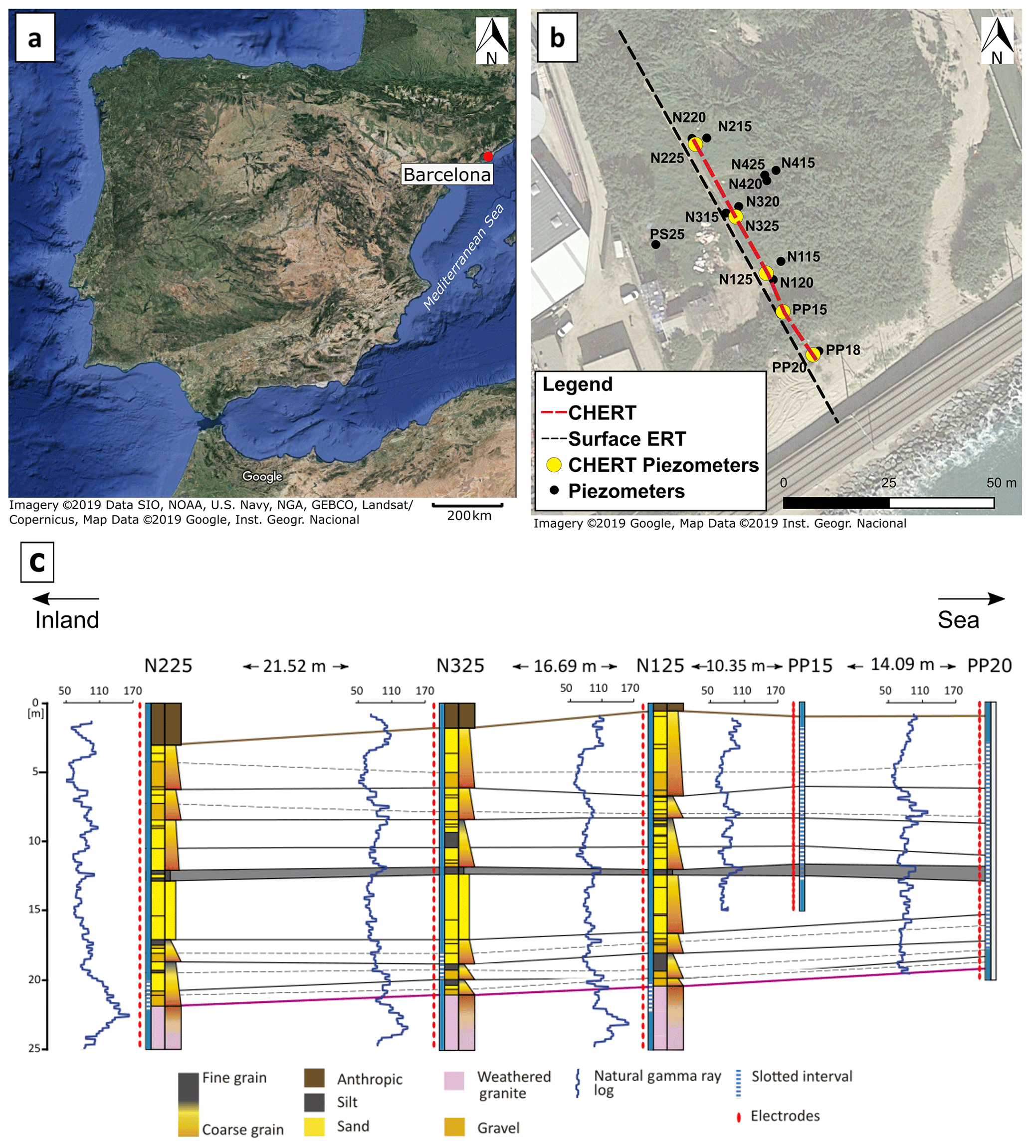
Figure 1(a) Location map of the Argentona site, some 30 km northeast of Barcelona, Spain. (b) Field spread of the Argentona site, installed piezometers (black dots), piezometers equipped with electrodes (yellow dots), surface ERT and CHERT transects. (c) Vertical cross section showing piezometers with screened depth, and location of the 36 electrodes in each well and stratigraphic correlation (modified from Martínez-Pérez et al., 2018). Two sandy aquifers are loosely separated by a silt layer at 12 m depth. The semiconfined aquifer is underlaid by weathered granite.
The Argentona site (Fig. 1) is located at the mouth of the “Riera de Argentona” (Argentona ephemeral stream), some 30 km northeast of Barcelona. The field site covers an area of some 1500 m2 and the mean elevation is 3 m. The Argentona stream only flows during heavy rainfall episodes that occur mainly in autumn. The climate is sub-Mediterranean. According to data from the Cabrils weather station, located 7 km northeast of the site, the mean annual precipitation since 2000 is 584.1 mm. Compared to most Mediterranean areas, the precipitation is more evenly distributed throughout the year, with the rainiest seasons being spring and autumn.
We have installed 16 piezometers in a cross-shaped distribution with the longest axis being oriented perpendicularly to the coastline (Fig. 1a). These include four nests (N1–N4) of three piezometers with depths of 15, 20 and 25 m (N115, N120, N125, etc.), screened over 2 m at the bottom. The distance from the closest piezometer (PP20) to the coastline is almost 40 m. The field site is located on a coastal alluvial aquifer that overlies a granitic basement (Fig. 1b). Core analyses reveal that the sediments are mostly unconsolidated. Martínez-Pérez et al. (2018) identify two sequences, located above and below a silt layer at −9 m a.s.l. The upper and lower sequences display a fining-upward pattern. The granitic basement was found at −17 to −18 m a.s.l. in piezometers N225, N325 and N125, with signs of intense weathering. A well-correlation profile was built from core descriptions supported by gamma-ray and induction logs. The silt layer at −9 m a.s.l. appears to be continuous along the main transect between piezometers N225 and PP20. Its continuity, especially towards and below the sea and its low permeability nature are yet to be defined. The present 2D conceptual model of the site is simple and several questions remain unanswered: is the silt layer continuous and impervious or is a significant water flow passing through it? Is the weathered granite an aquitard or another permeable unit given its strongly weathered nature? (see for example Dewandel et al., 2006). One of the goals of our time-lapse CHERT investigations is to contribute to answering these open questions and improve the conceptual understanding of the site.
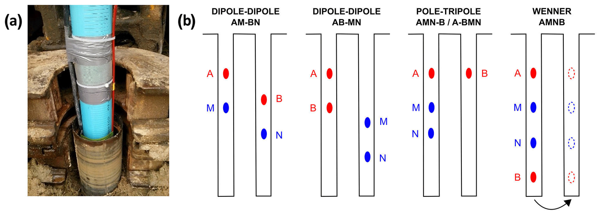
Figure 2(a) Stainless-steel meshes (electrodes) permanently fastened around PVC piezometers for the time-lapse CHERT experiment during piezometer installation. (b) Electrode configurations used in the survey. A total of 5843 measurements are recorded per CHERT in less than 30 min. Data are acquired sequentially by considering one pair of neighboring boreholes at the time. Four CHERT acquisitions are needed to build a complete CHERT, the whole 2D transect from boreholes N225 to PP20.
The objectives of the time-lapse CHERT experiments are to image SWI in order to improve the geological conceptual model, and to infer SWI dynamics. This requires installing metal electrodes in a corrosive saline environment, in which electrolysis due to current injection further accelerates the corrosion process and limits the lifetime of the installation. Therefore, addressing corrosion was one of the main concerns when designing the system and planning the monitoring experiments. The impact of corrosion on the electrode-functioning was tested in the laboratory before field deployment. The parts that are most sensitive to corrosion are the connection points between the mesh electrodes and the copper cables that bring current. Our strategy to delay corrosion at the connection points was to tie together the mesh and the cable, and to cover the connection point by a double silicone layer to prevent contact with water. In the laboratory, the electrodes showed signs of corrosion after 500 h of full contact with saline water (55 mS cm−1), under a constant current injection of 1 A at a frequency of 3 Hz. In our setup, stainless-steel mesh electrodes were permanently attached to the outside of the seven deepest PVC piezometers (Fig. 2a). When conducting a CHERT, the injected current is less than 1 A and the time of injection is a fraction of a second. Based on these laboratory test results, it was suggested that the instrumentation would last for at least 2 years, which was the minimum desired duration of the experiment.
All piezometers have 36 electrodes and the distance between electrodes is 70, 55 and 40 cm in the 25, 20 and 15 m depth piezometers, respectively. Numerical simulations by al Hagrey (2011) suggest that satisfactory resolution can be achieved using aspect ratios (horizontal distance between the boreholes and their depths) of up to 2 for different scenarios by fixing constraints about the resistivity structures during the inversion procedure. In the Argentona site, the aspect ratio for the different borehole pairs considered ranges from 0.6 to 0.8. Further details on the setup and installation are described by Folch et al. (2020).
When performing ERT, we measure an “apparent” resistivity that depends on the geometry of the acquisition. The apparent resistivity is related to measured electrical resistances:
where ρapp is the apparent resistivity, K is a geometric factor that depends on the electrode array and site characteristics, V is the voltage between two electrodes measured during current injection and I is the magnitude of the current flowing between another pair of electrodes. Any electrode configuration or array can, in principle, be used to perform ERT at the surface or between boreholes. For surface ERT, there are many well-established array types, such as Wenner, Schlumberger, dipole–dipole or pole–pole. For CHERT, several studies have sought to determine the most informative and cost-effective arrays for monitoring dynamic processes (Bellmunt et al., 2012; Zhou and Greenhalgh, 2000). Bellmunt et al. (2016) suggest that it is better to use different configurations (dipole–dipole, pole–tripole and Wenner) with different sensitivity patterns in order to obtain the maximum information about the subsurface. Moreover, given the corrosive environment in which the steel electrodes were installed, we decided to maximize the number of data measurements to ensure enough repeatability for the time-lapse inversion. The different configurations used were already described and assessed by Zhou and Greenhalgh (2000) and Bellmunt et al. (2016). Figure 2b shows the electrode configurations used at the Argentona site: dipole–dipole, pole–tripole and Wenner. Note that these data are acquired sequentially by considering one pair of neighboring boreholes at a time.
We use an optimized survey design that allows more than 5800 data points to be acquired in less than 30 min. After the installation of the electrodes around the casings (36 at each borehole), the data acquisition process was straightforward, with no need for large additional costs in maintenance or human working time. The equipment used was a Syscal Pro multi-channel (10-channel) system from IRIS instruments with 72 electrodes. The current injection time was 250 ms, and stacking of up to six measurements was done to meet data quality requirements. It took 2 h to complete the four CHERT acquisitions needed to cover the whole 2D transect from boreholes N225 to PP20. The combination of four such sections are referred to as a complete CHERT.
A total of 16 time-lapse datasets were collected during 2 years (five in 2015, eight in 2016, and three in 2017), corresponding roughly to a complete CHERT every 90 d. This relatively low sampling interval was partly motivated to decrease corrosion of the electrodes due to repeated current injections.
Data pre-processing was needed to remove anomalous and erroneous data points prior to imaging. Comparison of normal and reciprocal measured resistances is a common technique for appraising data errors (LaBrecque et al., 1996; Slater et al., 2000; Koestel et al., 2008; Oberdörster et al., 2010; Flores-Orozco et al., 2012). We follow the strategy proposed by Bellmunt and Marcuello (2011) for the quality control of the data based on the comparison between normal and reciprocal measurements. We chose a threshold of 10 % difference between the normal and reciprocal data in order to keep the measurement. Furthermore, the electrical contact resistance between the electrodes and the subsoil was checked before each data acquisition. Although the specific values of each pair of electrodes were not recorded, they were low in general. The deepest electrodes, in contact with the SWI, had contact resistance values in the order of 1 kΩ and the ones closer to the surface had values of a few tens of kilohms. Pseudo-sections of the apparent resistivities are easily created for surface ERT surveys, but there is no corresponding visualization technique for CHERT surveys. Instead, we plot geometric factors, apparent resistivities and data errors versus data number, to identify electrode configurations with anomalous values. Clearly, for time-lapse studies it is important to ensure that changes observed are due to subsurface processes, and not to changes in the survey setup. Consequently, the 16 datasets were scanned and compared to keep only identical electrode configurations.
For inversion, we make the common assumption that the bulk EC distribution is constant in the direction perpendicular to the complete CHERT transect. The corresponding 2.5D electrical inverse problem is solved on an unstructured mesh with tetrahedral elements using BERT (Boundless Electrical Resistivity Tomography) (Rücker et al., 2006; Günther et al., 2006) and pyGIMLi (Generalized Inversion and Modeling Library) (Rücker et al., 2017). The inversion algorithm inverts the log-transformed apparent resistivities, into a 2D log-transformed electrical resistivity distribution. The objective function to minimize is
where ϕd is the data misfit term, is the vector containing data residuals, d is a vector containing field data, f(m) is the forward response of the geoelectrical problem using model m and n is the order of the norm. In order to make the inversion less sensitive to data outliers, we apply a L1-norm mimicking scheme to the data misfit term using iteratively reweighted least squares (ILRS) (Claerbout and Muir, 1973). We assume uncorrelated data errors, so is a diagonal matrix with entries containing the inverse of the relative resistance errors. A relative error model with a 3 % mean deviation is further assumed. is the vector being penalized in the model regularization, with m the vector of estimated parameters and mref a vector of reference parameters. is the model regularization matrix. Smoothness operators are frequently used but are not suitable for capturing the sharp resistivity changes expected at the interface of the saltwater intrusion. We have chosen to define Cm as a geostatistical operator (Chasseriau and Chouteau, 2003; Linde et al., 2006; Hermans et al., 2012), containing site-specific information about how the resistive bodies are expected to correlate in space. Hermans et al. (2016) provide an example of how the inclusion of covariance information in ERT inversion improves the imaging of the target in terms of shape and amplitude, creating more realistic images. For this purpose, we use an exponential covariance model implemented in pyGIMLi by Jordi et al. (2018). The spatial support of the geostatistical operator helps to reduce the tendency of anomalies being clustered around the electrode region where sensitivities are high. The parameters used in the covariance model were chosen in agreement with the expected groundwater processes. Pore water is expected to flow through the horizontal layers shown in the stratigraphic correlation, so the variations that we expect to observe will be more correlated in the horizontal direction than in the vertical direction. The integral scales in the horizontal and vertical direction are 10 and 2 m respectively, the anisotropy angle is 90∘, and the variance of the logarithm of the resistivities was set to 0.25. The detailed description of this type of covariance model is found in, for example, Kitanidis (1997).
The minimization of ϕ is performed iteratively using the Gauss–Newton scheme. We start the inversion with a homogeneous model corresponding to the average apparent resistivity. In Eq. (2), λ is the regularization parameter. We apply an Occam-type inversion, in which we seek the smallest ϕm while fitting the data (Constable et al., 1987). We set λ to a high value at the first iteration and decrease it by 0.8 in each subsequent iteration. The iterative process is stopped when the data are fitted to the noise level.
To study variations in time, the simplest approach consists of independently inverting each dataset to analyze the evolution of changes. This approach may work when changes are large, but it is not considered state-of-the-art because inversion artifacts tend to be time independent (though not always; see discussion by Dietrich et al., 2018) and may mask actual changes. Singha et al. (2014) review time-lapse inversion as a way to impose a transient solution constraint through the analysis of differences or ratios in the data (Daily et al., 1992; LaBrecque and Yang, 2001), through the differentiation of multiple individual inversions (Loke, 2008; Miller et al., 2008), or through temporal regularization (Karaoulis et al., 2011). Daily et al. (1992) introduced the ratio inversion, in which data are normalized with respect to a reference model represented by a homogeneous half-space. The method allowed qualitative interpretation of resistivity changes, but made quantitative interpretation difficult. This motivated “cascaded inversion” (Miller et al., 2008), which consists of selecting as reference model the result of an initial inversion or baseline dataset. This approach removes the effects of errors and yields more reliable sensitivity patterns (Doetsch et al., 2012). The difference inversion by LaBrecque and Yang (2001) assumes that the changes from one acquisition to another are small, but this is not the case throughout the 2 years of monitoring at the Argentona site. In the newest approaches, a 4D active time-constrained inversion is applied simultaneously to all datasets (Karaoulis et al., 2011), penalizing differences between models. Although this is the most novel procedure for time-lapse inversion, it is computationally demanding. We have decided to apply the “ratio inversion”, solving for the updates of a reference model and thereby allowing us to account for the leading non-linear effects.
For data at time-lapse t,
where dt is the data vector at time t, f(mref) is the calculated forward response of the geoelectrical problem using a reference model mref and dref is the data vector of reference time tref.
The reference model for time-lapse inversion was built by inverting data from a complete CHERT and surface ERT from 8 September 2015. The surface ERT dataset consists of 1600 data points acquired along the transect shown in Fig. 1a. We used the Wenner–Schlumberger configuration with 72 electrodes and a 1.5 m electrode spacing. Inversion results are displayed in the next section in terms of bulk electrical conductivities, σb (the reciprocal of resistivities ρb).
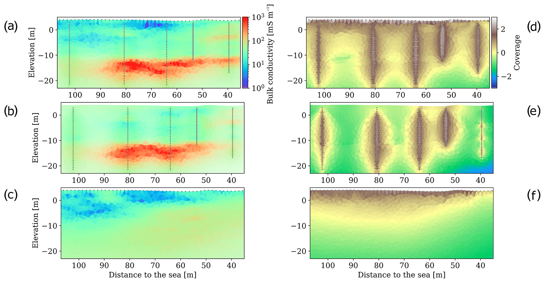
Figure 3Bulk electrical conductivity models obtained by the inversion of the CHERT and surface-based ERT data (a), the result when only considering the complete CHERT (b) and only the surface ERT (c) with the corresponding calculated coverages for each model (d–f). The complete CHERT model shows conductive anomalies (in red), which are not shown by the surface ERT model. The inversion of both datasets combines the coverages and yields an image with higher resolution near the surface and at depth (d).
5.1 Reference model
Inversion results of data used to establish the reference model are shown in Fig. 3. We display the bulk EC model obtained by the inversion of the CHERT and surface-based ERT data (Fig. 3a), the result obtained when only considering the complete CHERT (Fig. 3b) and only the surface ERT (Fig. 3c) next to the calculated coverages for each model (Fig. 3d–f). The bulk EC model obtained from the surface ERT campaign shows resistive layers in the first 5 to 10 m below the land surface, while the model obtained from the complete CHERT data alone is unable to resolve them. The complete CHERT, however, shows high conductive anomalies at depth. Also, the magnitude of the bulk EC below −10 m a.s.l. is higher in the complete CHERT model. These results confirm the expectations derived from the literature described in the introduction. Surface ERT is unable to accurately image the magnitude of saline regions at depth. Figure 3e and f display the coverage of the CHERT and surface ERT acquisitions computed using the cumulated sensitivity. The maximum coverage is attained near the electrodes. By combining the two datasets, the inverted bulk EC model has high sensitivity near the surface and at depth. The complementarity of the two surveys is well illustrated in Fig. 3d. For the reference model of the time-lapse inversion, we chose the inversion result from the complete CHERT dataset and the surface dataset (Fig. 3a).
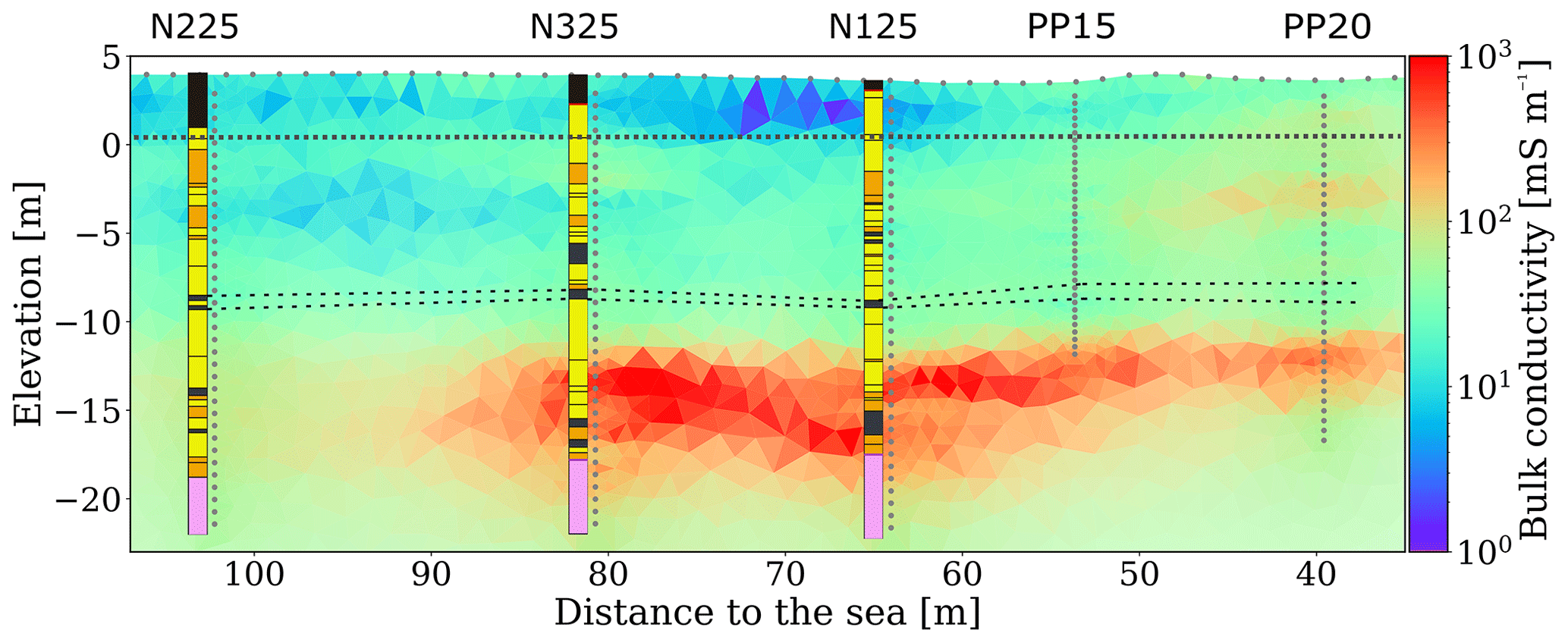
Figure 4Result from the inversion of surface and cross-hole ERT (dataset from 8 September 2015). Stratigraphic columns are shown to relate stratigraphic units with bulk conductivities. Gray dots represent the electrodes around the boreholes and on surface. The gray dashed line indicates the approximate groundwater table. The black dashed line indicates the silt layer. This cross section is used as reference model in the time-lapse inversion.
Figure 4 shows the reference model with the site stratigraphic correlation. The estimated bulk electrical conductivity ranges from 1 to 1000 mS m−1. A resistive layer of less than 5 mS m−1 is visible in the top 3 m, starting 60 m from the sea. This layer with low bulk EC is caused by the unsaturated zone; it coincides with the depth to groundwater (gray dotted line in Fig. 4) that usually varies between 0 and 0.5 m a.s.l. The thickness of the unsaturated zone is resolved thanks to the surface ERT data. The bulk EC grows to a mean value of 50 mS m−1 below the water table in the shallow aquifer from 0 to −10 m.a.s.l. Conductivity grows further, exceeding 500 mS m−1, below −10 m.
Bulk electrical conductivity values above 200 mS m−1 can here be conclusively attributed to the presence of seawater in the pore space. We see an upper conductive anomaly of some 100 mS m−1 in the unconfined aquifer above −5 m a.s.l. towards the sea (from 35 to 50 m to the coast). We attribute this anomaly to beach sediments saturated with a mixture of fresh and saline water. The upper anomaly vanishes inland before piezometer PP15. The second conductive anomaly, below −10 m a.s.l., extends from 35 to 90 m to the coast, and it vanishes before reaching piezometer N225. Poor imaging resolution is not expected at this depth, so we must consider the possibility that lithological heterogeneity or lower water salinity causes the change in bulk EC in the lower aquifer. In the bottom part of Fig. 4, bulk EC decreases where the top of the granite is found in piezometer N125.
The reference model and stratigraphic units provided insights pertaining to the interpretation of subsurface processes. Time-lapse changes will help confirm whether conductivity anomalies in the reference model are related to fluid dynamics or to geologic structures.
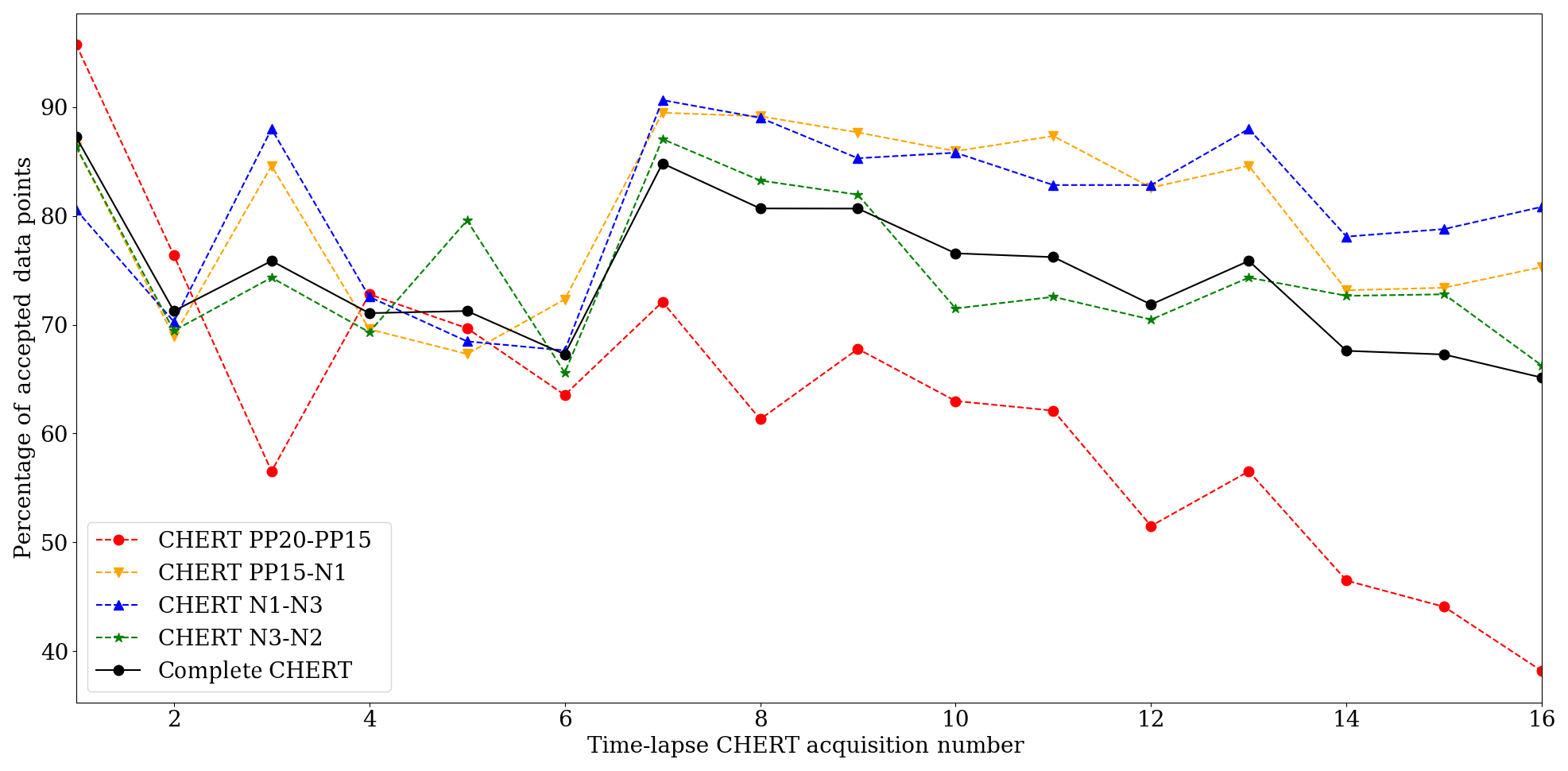
Figure 5Percentage of accepted data points in each CHERT, after quality control during data pre-processing. Note the decrease in the amount of accepted data with time, most likely due to corrosion of the electrodes, particularly in the PP20-PP15 panel, which is located the closest to the sea.
5.2 Time-lapse results
Figure 5 shows the time evolution of the data percentage that satisfies the constraints on data quality (less than 10 % percent of difference between normal and reciprocal measurements). The panel between boreholes PP20 and PP15 is the one that suffers the most from discarded data, likely due to its proximity to the coast, and it is the zone where lower resistivities cover a thicker vertical zone. The decrease in data quality with time is probably related to corrosion processes of the electrodes in contact with marine water. The quality control after each acquisition, plus the identical geometry constraint for the time-lapse inversion, reduced the dataset to 2677 identical measurements that were extracted from each complete CHERT.
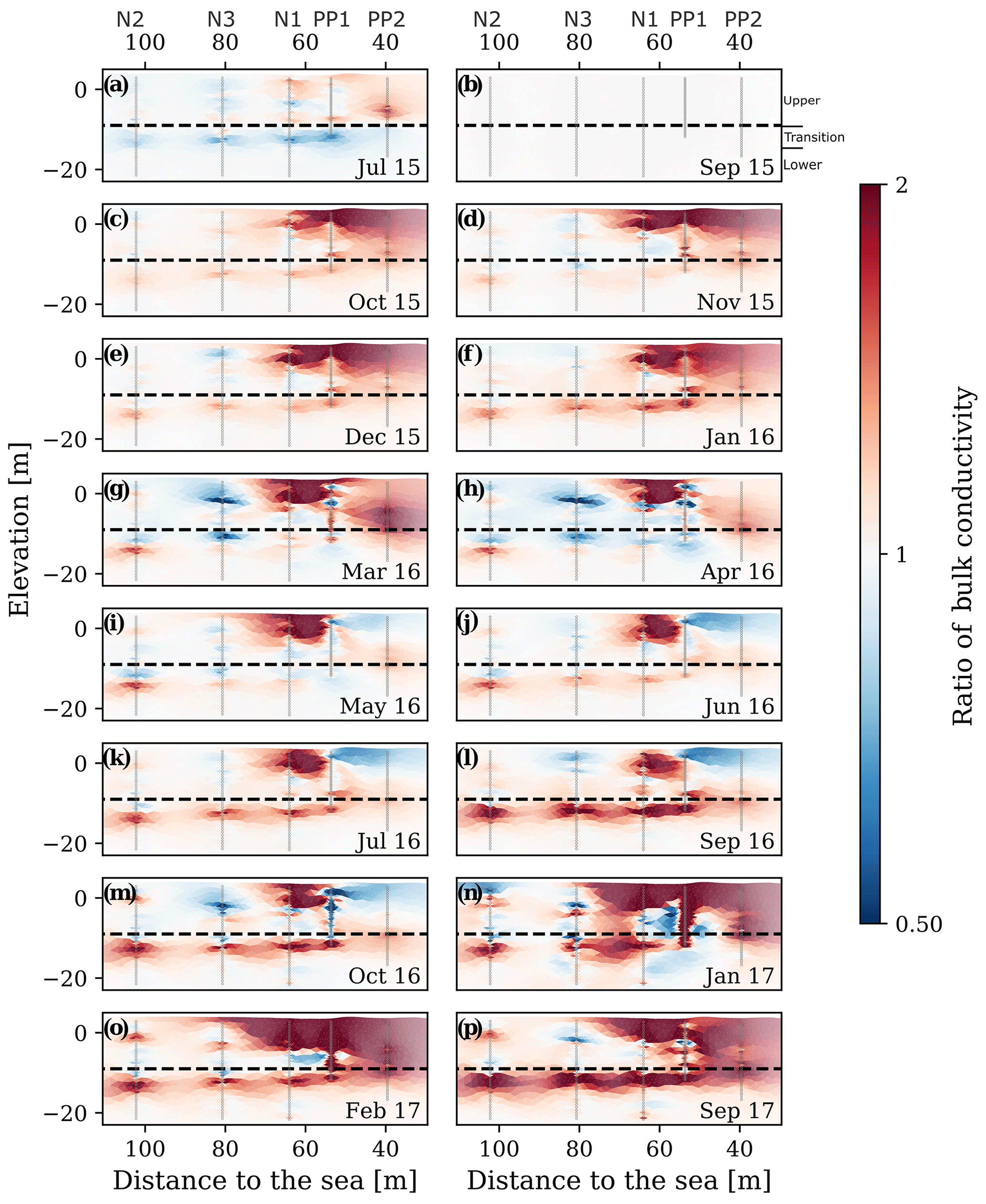
Figure 6Results from the time-lapse inversion of 16 complete CHERT acquired over 2 years (July 2015 through September 2017). Images display the ratio of bulk electrical conductivity with respect to September 2015 (a brownish area implies higher EC and, therefore, salinity than in September 2015). The silt layer is indicated with a dashed line. Note the increase in bulk EC in the upper-right side (<80 m of distance to the sea), and along a line just below the silt layer, indicating a rise in the saltwater interface.
Time-lapse results are displayed in Fig. 6 as the ratio between each bulk EC model and the bulk EC of the reference model (September 2015). The color scale in the figure varies from a twofold increase (dark red) to a decrease by half (dark blue) in bulk EC with time. The color scale does not show the minimum and maximum magnitude of the variations; it was chosen to highlight major changes in the 2 years of monitoring. In the imaging process, the use of a geostatistical operator in model regularization helped in removing the boreholes' footprint in the bulk EC models, but these remain in the ratio images due to the high sensitivity of the method near the electrodes. Figure 6a (ratio of September to July 2015 ECs) shows an increase in bulk EC during summer 2015. That is, EC is smaller in July than in September, which suggests advancement of salinity. From October 2015 to March 2016 (Fig. 6c–g) an increase is successively observed near PP20, reaching 70 m from the sea. In March, April and May 2016 (Fig. 6g–i), a decrease in bulk EC is observed in both aquifers. Complete CHERT values from June 2016 to September 2017 (Fig. 6j–l) show successive increases in the conductivity of the semiconfined aquifer, below −10 m a.s.l. In 2017 (Fig. 6m–l), a highly conductive anomaly reappears in the upper-right part of the time-lapse ratio images between nest N3 and borehole PP20. This is the largest anomaly captured by the experiment in size and magnitude. In the last ratio image between September 2017 and September 2015 (Fig. 6l), the increase in bulk EC in the study area is clearly observed.
We analyze the origins of long-term and short-term changes described in the previous paragraph by correlating them with precipitation and wave activity data. The precipitation and the wave activity data are here used as a proxy to indicate the likely timing when a significant freshwater recharge occurred and when water from large waves might have formed seawater ponds at the surface.
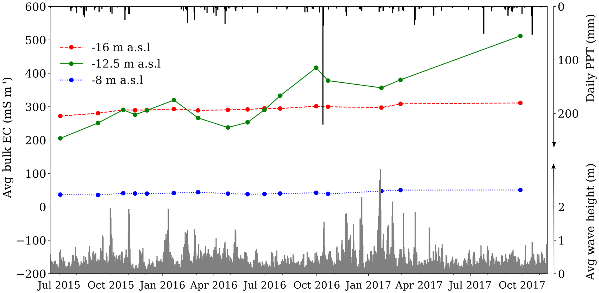
Figure 7Average conductivities extracted from the inverted models, at −8 m a.s.l. (blue), −12.5 m a.s.l. (green) and −16 m a.s.l. (red). Precipitation (PPT) data from Cabrils station and simulated significant wave height time series are displayed. The points indicate times of CHERT campaigns. Note that acquisitions were made before and after the 220 mm precipitation event of 12 October 2016. Significant seasonal fluctuations and an overall increase in EC can be seen in the upper part of the semiconfined aquifer (elevation of −12 m a.s.l.) but are negligible in the lower portion of both the shallow unconfined aquifer (−8 m a.s.l.) and the semiconfined aquifer (−16 m a.s.l.).
Figure 7 displays the average conductivity of the inverted model at −8, −12.5 and −16 m a.s.l. In this figure we also display daily precipitation data from the Cabrils Station, located 7 km northeast of the site. Precipitation data (inverted y axis) show two relevant features: (1) important precipitation events can occur in one day (e.g., 220 mm in October 2016); (2) the rainiest periods during the 2 years of monitoring consistently occurred in the fall and spring. The winter and summer of 2016 were the driest periods. Wave-related data (normal y axis) are obtained from a numerical model called SIMAR 44 (Pilar et al., 2008). The numerical model is calibrated using data from wave buoys distributed along the Catalan coast. Wave numerical models have limitations and tend to underestimate wave height near the coast, but they give general insights about the wave activity (WAMDI Group, 1988). In Fig. 7, we show the significant wave height from the numerical model. Significant wave height (Hs) is defined as the average height of the highest one-third of waves in a wave spectrum (Ainsworth, 2006), and it is the most commonly used parameter because it correlates well with the wave height that an observer would perceive. The wave data show increased wave heights in Autumn 2015, January 2016 and winter 2017. These periods correspond to the appearance of a superficial conductive anomaly in the upper part of the time-lapse images.
The plots of average bulk EC in Fig. 7 capture the evolution of the conductivity in the unconfined and the underlying semiconfined aquifer over time. The mean bulk EC of the upper portion of the lower aquifer (at −12.5 m a.s.l.) displays a more than twofold increase (from 200 to more than 500 mS m−1) in the 2 years of monitoring. We can also observe cyclic variations throughout the year. In contrast, both fluctuations and overall variation are very small at both the shallow (bulk EC around 20 mS m−1) and greater (some 300 mS m−1) depths.
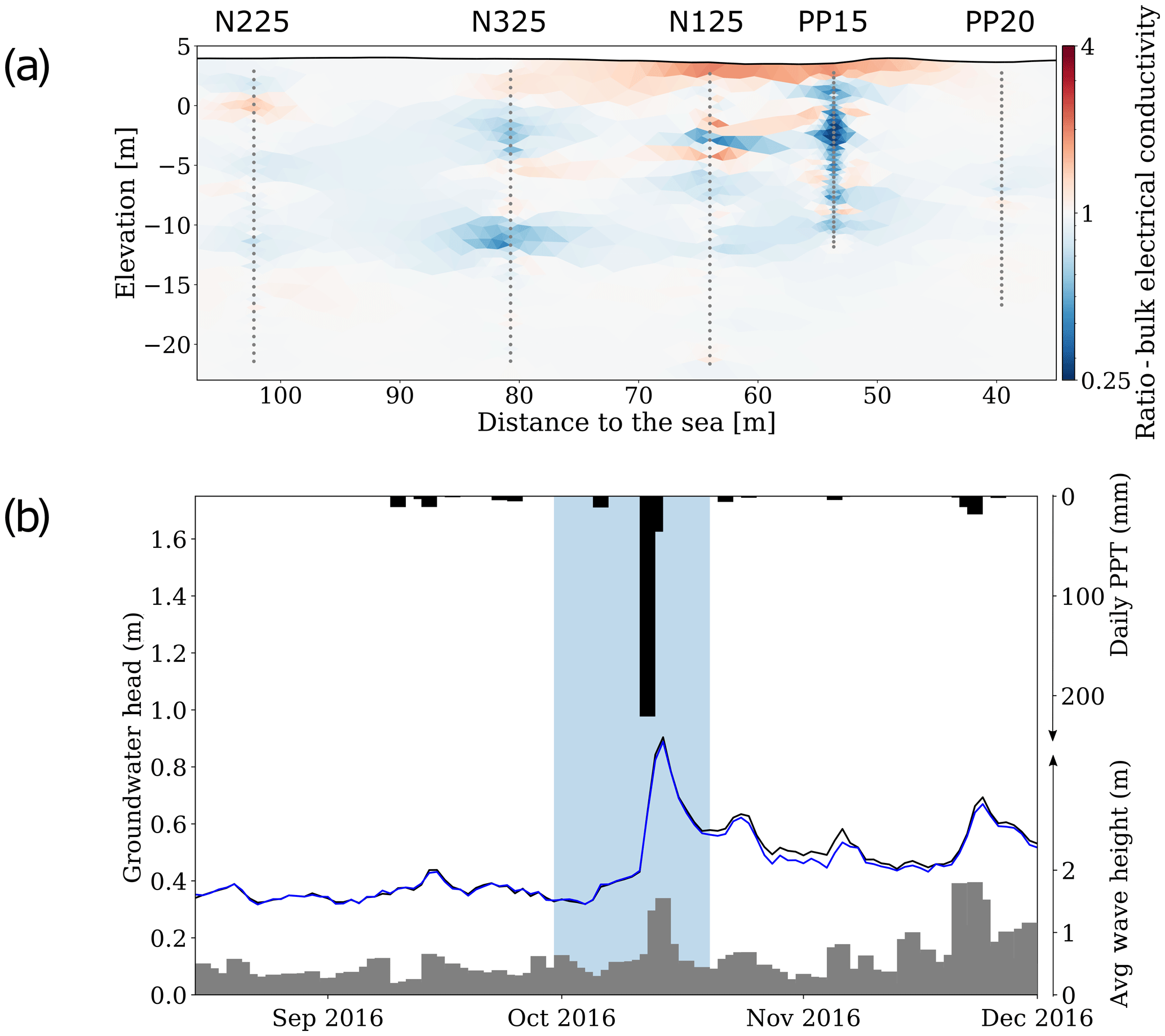
Figure 8(a) Ratio between the bulk electrical conductivity model of 30 September and 21 October 2016. The heavy rain occurred on 12 October 2016. The image shows a decrease in conductivity in the unconfined and semiconfined aquifer and a conductivity increase in the unsaturated zone on both sides of nest N1. The decrease in conductivity observed along borehole PP15 is attributed to freshwater infiltration due to borehole construction. (b) Time series of groundwater level in boreholes N115, average significant wave height (gray bars) and precipitation (black bars). Highlighted is the heavy rain event of 220 mm that occurred on 12 October 2016. The event was accompanied with an increase in groundwater level and in significant wave height.
In order to assess the impact of a heavy rain event at the site, we have computed the ratio of the CHERT bulk EC models from 30 September and 21 October 2016, 11 d before and 9 d after the heavy 220 mm precipitation. The color scale chosen for the Fig. 8a differs from previous figures to improve visualization of the bulk conductivity variations. Figure 8a displays the conductivity ratio image, which reveals a decrease in the conductivity throughout the saturated zone, both above and below the −10 m a.s.l. silt layer, and an increase in the unsaturated zone, above the 0 m a.s.l., between nest N3 and PP20. No difference is observed below −15 m a.s.l. The decrease in conductivity observed along borehole PP15 is most likely related to water flowing along the borehole (the site was flooded). Heads measured in piezometers N115 (black) and N120 (blue) are shown in Fig. 8b, showing that hydraulic heads increased 60 cm in nest N1 during the rain. Rain was accompanied by an increase in the significant wave height. After 10 d, when the complete CHERT was acquired, groundwater level had already dropped by 30 cm.
A clear change observed in time-lapse images of Fig. 6n–p is the increase in bulk EC in the shallow layers during the winter of 2017. This increase in bulk EC occurs at a time of higher wave activity, as shown by Fig. 7. To quantify the amount of the increase in conductivity, we compute the ratio of the bulk EC of CHERT from October 2016 (the last tomography before winter) and February 2017 (a tomography during winter and the high-wave period). The result from the ratio is displayed in Fig. 9a. Again, the color scale of the figure is adapted to better visualize the variations. EC increased by 200 %–500 % from 80 to 35 m from the coastline, between nest N3 and borehole PP20. The increase in conductivity observed along borehole PP15 is, again, most likely related to water flowing along the borehole. Figure 9c shows the recovery of the bulk EC in the shallow layers around PP20 in September 2017.

Figure 9(a) Ratio of October 2016 to February 2017 CHERT ECs. (b) Extraction of CHERT bulk EC profiles along PP20. The winter period with higher significant wave heights is marked by a twofold increase in bulk electrical conductivity values from the coastline until 90 m from the coastline. The extractions in (b) show the bulk EC in the upper layers during winter (200 mS m−1), and the recovery 6 months after winter (100 mS m−1). The extractions also evidence the increase in conductivity in the lower aquifer.
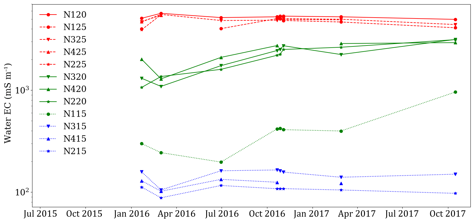
Figure 10Water electrical conductivity measurements taken on water samples from piezometers in nests N1, N2, N3 and N4. The piezometers are grouped according to the elevation of the screened intervals: “upper” (blue, −7 to −10 m a.s.l.), “transition” (green, −11.5 to −13.5 m a.s.l.) and “lower” (red, −15.5 to −18.5 m a.s.l.), where EC is that of seawater.
Measurements of water EC from water samples are displayed in Fig. 10. Piezometers from nests are screened at different depths, and we have grouped them in three categories: N115, N215, N315 and N415 are in the “upper” group (colored in blue), because the screening depth is above −10 m a.s.l.; N220, N320 and N420 are in the “transition” group (colored in green), with the screen around −12.5 m a.s.l., thus, just above the saltwater intrusion; and N120, N125, N225, N325 and N425 are in the “lower” group (colored in red), with the screen below the transition zone, where saltwater is considered to be concentrated. Similar to the plots of average bulk EC from complete CHERT in Fig. 7, the major changes occur in the “transition” group, with an increase in water EC of 300 %, from 1000 to 3000 mS m−1 in the 2 years of monitoring. Apart from the increase in water EC observed in N115 (screened interval at −9.9 m a.s.l.), no clear variations are observed in the “upper” and “lower” groups. Note that N120 has higher conductivity values than N125, which suggests that a freshwater source is present or a desalination process is occurring below −18 m a.s.l.
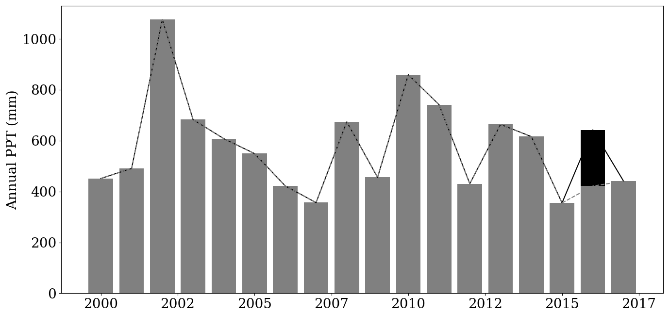
Figure 11Annual precipitation since 2000 from Cabrils weather station, 7 km northeast from the site. Average precipitation is 584.1 mm (dashed line). Note that the monitoring period is below the average. The black bar in 2016 represents the 220 mm rain event of 12 October, which probably produced relatively less recharge than typical rainfalls.
Figure 11 displays the precipitation history recorded at the Cabrils station, 7 km northeast from the site. The annual precipitation from 2000 to 2017 is plotted in gray. The black bar of year 2016 refers to the heavy singular 220 mm rain event, which causes that year to look wet but produces floods rather than proportional recharge. Average yearly precipitation since 2000 is 584.1 mm. The driest year of the sequence was 2015, with only 355 mm of precipitation (38 % lower than average). Actually, rainfall was below the long-term average during the last 3 years of monitoring. The 2015 to 2017 drought is the likely cause for the overall increase in the aquifer bulk electrical conductivity, due to the decrease in freshwater recharge.
The reliability of bulk electrical conductivity models obtained with the CHERT experiment can be evaluated using other independent datasets. Induction logs (ILs) acquired at the Argentona site also provide bulk EC models. Induction logs were done using the GEOVISTA EM-51 electromagnetic induction sound. Figure 12 displays a comparison of the bulk EC from ILs along piezometers N2, N4, N3 and N1 (from left to right) and extractions from the complete CHERT conductivity models along the same piezometers. N4 is not on the complete CHERT transect, but as we neglect heterogeneity perpendicular to the transect, we assume nest N4 is comparable to nest N3. ILs were not performed in the 25 m deep piezometers because the stainless-steel electrodes installed outside the casing severely corrupted the recorded signal. Instead, they were performed in neighboring 20 m deep piezometers that do not contain any electrodes. ILs from May 2015 (light blue), before the beginning of the CHERT experiment, are available for all piezometers. They are compared with the CHERT conductivity model from July 2015 (dark blue). In Fig. 12c, an IL from July 2016 in nest N3 is compared with CHERT conductivity model from the same month. In Fig. 12b, an IL from October 2017 in nest N4, conducted 2 weeks after the end of the CHERT experiment, is displayed with the CHERT conductivity model from September 2017 of nest N3. The CHERT conductivity model can be well correlated with the IL from all piezometers. There are differences in the magnitudes of the bulk EC, but both methods agree on the location of the transition zone, from −10 to −12 m a.s.l.
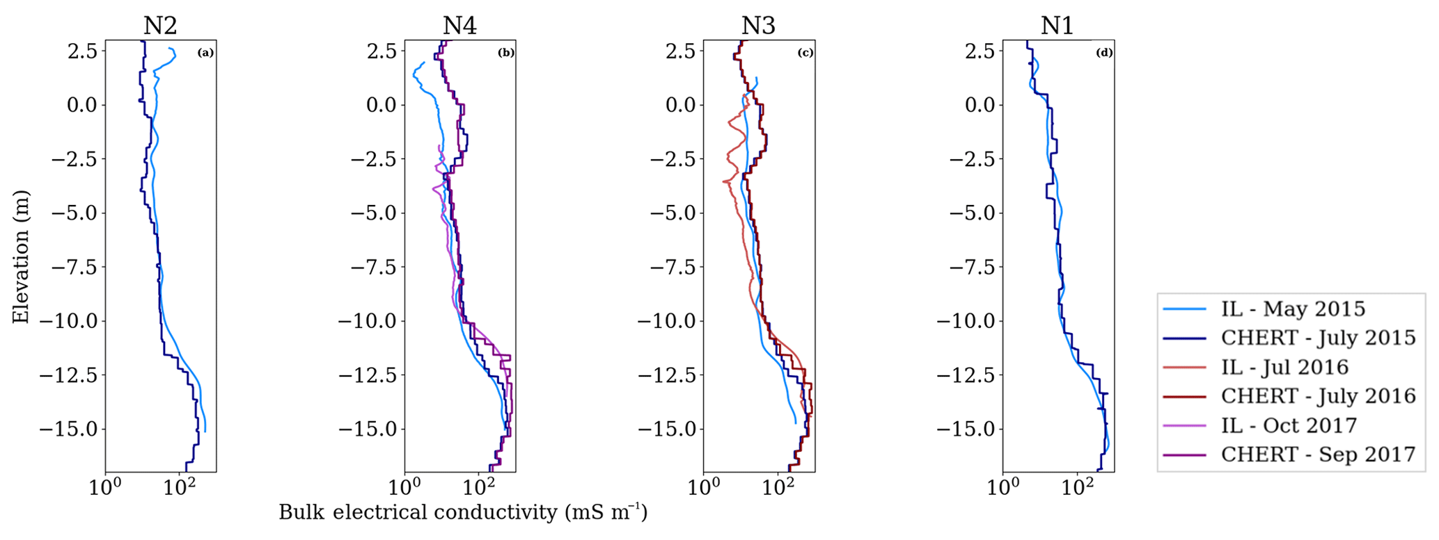
Figure 12Comparison of bulk electrical conductivity models obtained from induction logs and CHERT along piezometers in nests N2 (a), N4 (b), N3 (c) and N1 (d). The CHERT logs were extracted from the CHERT bulk EC models along the boreholes.
6.1 Surface ERT vs. CHERT
Surface ERT reflects quite accurately the thickness of the unsaturated zone and the location at which the water becomes more saline, but it is impossible to image the difference between the transition zone and the actual saltwater intrusion. Using only the surface ERT bulk conductivity model, one could argue that SWI in the Argentona site displays the paradigmatic saline wedge shape of Abarca et al. (2007) or Henry (1964). Instead, the CHERT data model suggests two conductive anomalies, one in the unconfined aquifer towards the sea, and one in the semiconfined aquifer below the −10 m a.s.l. silt layer.
An important magnitude difference is observed between surface ERT and complete CHERT bulk EC models. The surface ERT model shows much lower bulk EC in the saltwater zone than the complete CHERT model. Studies trying to link hydrological and geophysical models in coastal aquifers (Huizer et al., 2017; Beaujean et al., 2014; Nguyen et al., 2009) have encountered difficulties using surface ERT-based models due to insufficient resolution at the depth of interest. This lack of resolution causes the underestimation of water EC, and thus of water salinity. The differences in the models shown in Fig. 4a suggest that surface ERT is not able to correctly capture the conductivity contrasts in the subsurface. This finding is confirmed by the validation of the CHERT bulk EC models with induction logs (Fig. 12).
6.2 Reference model: link between bulk EC and geological conceptual model
The complete CHERT produces a quite clear picture of the link between the bulk EC model and the stratigraphic units. We can explain the presence of two saline bodies with the presence of a continuous semiconfining layer, and the existence of up to three different aquifer layers. This is relevant by itself because it was unexpected. The only geologic feature is a relatively minor but apparently continuous silt layer, which we originally discarded as relevant. Bulk EC imaging suggests that this layer may play an important role. The transition zone is not located at the depth of the silt layer. This silt layer is the one separating the unconfined from the semiconfined aquifer. It is not, however, separating the freshwater from the saltwater. The saltwater intrusion zone begins 2 to 3 m below the silt layer, thus suggesting that a significant flux of freshwater occurs below this layer. This result is consistent with sandbox experiments of Castro-Alcalá (2019), who found that relatively minor heterogeneities may cause the saltwater wedge to split.
In addition, CHERT allowed us to improve the visualization of the SWI in comparison to traditional hydrology monitoring methods. Indeed, using traditional methods the silt layer would have been completely discarded as relevant, but the CHERT made possible the visualization of a non-monotonic salinity profile that confirms the importance of the heterogeneity. Specifically, salinity profiles in fully screened boreholes (such as PP20) are always monotonic (EC increases with depth) and rarely reach seawater salinity. Our imaging points out that actual salinity is non-monotonic and leads to the suggestion that it is the flow of buoyant freshwater within the borehole what explains both the observed step-wise increase in traditional salinity profiles and the fact that salinity is below that of seawater. The process is described by Folch et al. (2020) and by Martínez-Pérez et al. (2018), but visualization is only possible by ERT (and specifically CHERT) or electromagnetic methods (e.g., induction logs).
Weathered granite was found in the cores at the bottom of N1, below −17 m a.s.l. At this depth, the magnitude of the CHERT bulk EC model decreases. We can, thus, infer that the decrease in bulk EC at the base of piezometers N325 and N225 is related to the continuity of the crystalline formation. Loss of resolution below PP20 and PP15 does not allow us to infer anything about the presence of weathered granite towards the sea. From the available data, we conclude that the decrease in bulk EC observed in the images has two causes: first, an important change in lithology from gravel to weathered granite; and, second, a decrease in water EC observed in the water samples from N125, with respect to the water sample from N120 (Fig. 10). The water EC values from N125 samples suggest that pore water is a mixture of fresh- and saltwater. The granite is, most likely, not an impervious boundary for mixing processes, but merely another source of heterogeneity in the system. The existence of freshwater from bottom layers of the model is yet to be explored, but it is consistent with the findings of Dewandel et al. (2006), who described frequent highly transmissive zones at the base of the weathered granite in numerous sites around the globe.
The conductive anomalies fade while moving away from the sea. Above −10 m a.s.l., the small conductive anomaly stops before PP15, and is no longer present around N325. Below −10 m a.s.l., the conductive anomaly is present until N325, but is weaker around N225. Due to the distance between piezometers N225 and N325, the sensitivity of the CHERT in this panel is lower than for the rest of the borehole pairs and the decrease in the bulk EC conductivity may be related to it. Nevertheless, this diminishing trend in the bulk EC reference model coincides with water EC values from piezometer N320 being slightly higher than water EC from piezometer N220. We identify a vertical mixing zone, but also a lateral mixing zone between nests N3 and N2.
In summary, by comparing the CHERT bulk EC model, water EC measurements and the site stratigraphic columns, we are able to highlight several features. (1) The resistive anomaly observed at the top is certainly related to partial water saturation. (2) The seemingly continuous silt layer found at −9 m a.s.l. in boreholes N225, N325 and N125 does not represent a freshwater–seawater boundary. The freshwater–seawater boundary appears 2 to 3 m below, which implies that the silt layer is a semiconfining layer and freshwater discharges below. (3) There are not one but two saline bodies, one in each aquifer. The lower one is a traditional one, but the upper one is more complex and will be discussed in Sect. 6.4. (4) The conductivity value of the most conductive anomaly below −10 m a.s.l., interpreted as seawater-bearing formations, decreases at the top of the weathered granite. This decrease in bulk EC is explained by the reduction of water EC, and by a reduction in bulk EC due to the larger electrical formation factor of the granite. (5) CHERT bulk EC models show the location of a vertical transition zone, and also the extent of a lateral transition zone.
6.3 Time-lapse study: long-term effects
6.3.1 Seasonality: the natural dynamics
The time evolution of the average bulk EC displayed in Fig. 7 shows that there are months with a decrease in bulk EC conductivity and months with an increase in bulk EC conductivity. These months are correlated with rainy and dry periods, and also with the occurrence of storm surges. During summer and beginning of autumn, the conductivity increases slowly until the rain period starts; in autumn, during heavy rains, conductivity decreases; during winter months, conductivity increases due to sea storms; in spring, conductivity decreases, and it reaches its lowest point before the dry summer period begins again. In the deeper areas where seawater is already in place, average bulk EC does not show important variations.
6.3.2 The drought: long-term salinization
The time-lapse ratio image from September 2017 (Fig. 6l), the average bulk EC at −12.5 m a.s.l. (Fig. 7) and the water EC measurements in the transition zone (Fig. 10) indicate a clear increase in bulk EC in the lower aquifer since the beginning of the experiment.
We conjecture that this increase in water salinity is linked to the drought that started in 2015 and had not yet ended by November 2017. In recent years, drought occurs every 8 to 10 years and lasts a few years. This is visible in Fig. 11 in the years 2006–2007 and 2015–2016–2017. The effect of the decrease in freshwater recharge by rainfall is observed in the experimental results, in the form of salinization of the aquifers at a distance of 100 m from the coastline. This result is corroborated by water EC from water samples taken at the piezometers. The overall increase in bulk EC is attributed to an overall increase in water EC. While this is not surprising, what may come as a surprise is the relatively slow response of salinization of SWI to weather fluctuations. No steady regime has been reached after 3 years and salinization continues.
6.4 Time-lapse study: short-term effects
6.4.1 The heavy rain: a freshwater event
A 220 mm – a third of the region's average annual precipitation – rainfall event lasting less than a day occurred on 12 October 2016. It was a catastrophic event that created human and material losses due to flooding. The Argentona stream is an ephemeral stream that carries water a few days each year during monsoon-like rains, typically between September and December. A rainfall of this magnitude floods the Argentona stream, and the entire experimental site.
Do the CHERT images capture the effect of the heavy rain in the coastal aquifer? Figure 8a displays the difference in conductivity obtained by the tomography from 11 d before the rain and 9 d after the rain. The bulk EC ratio image reveals a decrease in the bulk EC in both upper and lower aquifers. In October 2016, according to Fig. 7, the increase in bulk EC that was taking place was interrupted after this heavy rainfall.
To understand the change in bulk EC, we must think in terms of water masses. When an important precipitation event occurs, freshwater flows through rivers and streams towards the sea. Inland, some freshwater infiltrates into the subsurface, pushing in situ water masses down and to the sides. The displacement of “old water” creates space for the newly infiltrating fresh rainwater, and this movement enhances mixing processes. Offshore, surface and submarine groundwater discharge is occurring at the same time. The observed change in bulk EC is most likely the result of the mixture of old saltwater with rainwater in the aquifer, which creates a new water, that is still saline but less so than before the rain event. However, despite the rainfall magnitude, EC changes were neither dramatic nor long lasting.
The effect of the heavy rain that lasted only a few hours supports what was said in the drought section about this rain not being representative of the region's precipitation. One sudden episode, even of this magnitude, is not enough to make a significant difference in the seawater intrusion pattern and in the aquifer’s long-term salinization.
6.4.2 The storm: a saltwater event
From July 2015 to October 2016, CHERT experiments had conveyed that the most conductive anomaly was concentrated below the silt layer, but another strong conductive body appeared between nest N3 and borehole PP20 early in 2017.
The traditional SWI paradigm (Abarca et al., 2007; Henry, 1964) suggests that it is the freshwater head that drives the seawater–freshwater interface movement. When heads rise, the interface moves down and seawards because freshwater pushes saltwater seaward. When the groundwater table falls, the opposite occurs, and the seawater interface moves up and inland. The work by Michael et al. (2005) explains how other mechanisms, besides seasonal exchanges, can promote seawater circulation enhancing the seawater intrusion and mixing. According to Michael et al. (2005), some of these mechanisms are tides, wave run-up on the beach and dispersion of saline water into freshwater discharge. In the Mediterranean Sea, tidal forcing is not a cause of important change in heads because the tidal amplitude is small (<20 cm). Wave action and wind could drive changes in the sea level and thus in groundwater heads, but these effects are not long lasting.
A recent study by Huizer et al. (2017) about monitoring salinity changes in response to tides and storms in coastal aquifers showed, through surface ERT experiments, as well as flow and transport simulations, that storm surges can have a strong impact on groundwater salinity. In time-lapse images of the Argentona site, storms seem to be enhancing the conditions for seawater to move inland, through the most superficial layers (Fig. 9a), and further infiltrate the soil from the surface through piezometer PP15, which is fully screened, and between nests N1 and N3. However, salinity increases from the top, rather than from an interface. Therefore, we conclude that these changes in salinity are the result of storm surges, rather than from interface dynamics. In fact, 6 months later (Fig. 9c), the unconfined aquifer has recovered, which implies a more dynamic system in the superficial layers. The CHERT experiment seems to constitute a good tool for the monitoring of such phenomena near the coast related to tides, wave run-up and submarine groundwater discharge.
6.5 Model validation
Differences between bulk EC models obtained from induction logs and CHERT are attributed to the differences in location and in time of acquisition, considering they were performed neither at the same time nor at the exact same location.
The comparison of the bulk EC model with other independent data sources was very important to prove the reliability of the CHERT experiment. The use of other types of data such as induction logs and water EC from water samples have helped in increasing the confidence in the capabilities of the CHERT experiment for monitoring coastal aquifer dynamics. Water samples are taken only from screened piezometers or with the use of sophisticated isolating equipment. With water samples we can observe the increase in water EC in time and in space, but we cannot know the depth of the interface or the lateral variations between wells. Induction logs reproduce similar data than the CHERT experiment, but only along piezometers. Interpolation techniques must be applied to IL data to obtain a 2D image. The CHERT experiment involves real interaction between boreholes. Furthermore, although sensitivity is concentrated around the electrodes (Fig. 4), we would like to stress that ERT (surface- or borehole-based) have sensitivity to the electrical conductivity outside of the array (so-called outer-space sensitivities) as studied by Maurer and Friedel (2006).
6.6 The CHERT experiment
The CHERT experiment, contrary to surface ERT, is an invasive procedure because it needs the installation of boreholes, which may affect local dynamics. For example, the vertical anomalies along piezometer PP15, better observed in Figs. 8a and 9a, are attributed to fluid flow through the annular space between the borehole and the formation. Borehole measurements are, nonetheless, necessary for subsurface exploration. We suggest an additional consideration when planning the position of the boreholes to use CHERT. A key point to consider when defining a CHERT experiment is the aspect ratio between the horizontal distance of the boreholes and the maximum vertical distance between the electrodes located in each borehole (e.g., LaBrecque et al., 1996). Ideally, we would look for small values of the aspect ratio, but the location of the boreholes was conditioned by several factors including logistics and requirements for other monitoring methods as well as experiments planned at the experimental site. Furthermore, there is a trade-off with the overall investigation area implying that larger borehole spacings are sometimes motivated. Beyond this, both the geology (Figs. 1c and 4) and the SWI display significant lateral continuity so that vertical resolution is more critical than the horizontal one. This is achieved by imposing stronger regularization constraints in the horizontal than in the vertical direction. The use of an optimized protocol to acquire a complete dataset in the least amount of time is recommended to capture dynamic processes with changes happening in a smaller time step. This was not the objective of the CHERT monitoring experiment in Argentona from 2015 to 2017, but it is feasible (taking into consideration that metal corrosion will be accelerated by the injection of electric current, implying that the life of the instrument will certainly be shorter). Although surface ERT does not have enough resolution for the depth of interest, the combination of CHERT with surface ERT is suggested to understand the most superficial layers of the subsurface. Future work will include hydrological modeling of density-dependent flow and transport at the Argentona site in order to reproduce the observed bulk electrical conductivity changes observed with the CHERT experiment. It is anticipated that this model can be used to predict future changes in the system.
The monitoring experiment using CHERT at the Argentona site, from July 2015 to September 2017, was successful in several aspects, regarding both geophysical imaging and SWI understanding:
-
The joint use of CHERT and surface ERT increased the initial model resolution compared with using surface ERT only. Comparison of CHERT inversion to salinity profiles from induction logs is excellent and validates the methodology.
-
The increase in resolution allowed us to image unexpected salinity changes both in the upper layers, and the lower layers with only limited loss of resolution with depth despite the high salinity of water.
-
Imaging of spatially fluctuating salinity has led to explaining the paradoxical salinity profiles often recorded in fully screened wells (step-wise increase but without reaching seawater salinity) as due to deep freshwater flowing up inside the well and mixing.
-
Time-lapse CHERT captured long-term and short-term conductivity changes. Long-term changes included (a) seasonal fluctuations of groundwater flux that cause the seawater–freshwater interface to move seawards during periods of high flux or landwards during periods of low flux, and (b) the long-term salinization of the lower aquifer due to an intense drought in the study area during the monitoring period. Short-term changes included (a) a decrease in conductivity related to a heavy individual rain event of 220 mm of precipitation (a third of the annual average rainfall) in only one day, and (b) an increase in conductivity in the beach area, coinciding with storms that caused enhanced wave activity.
In short, employing CHERT at the Argentona site proved to be a cost-effective and efficient tool to shed light on seawater intrusion dynamics through the analysis of bulk formation conductivity.
Datasets and instructions to reproduce the CHERT experiment results are available for the scientific community through the H+ database at http://hplus.ore.fr/en/palacios-et-al-2020-hess-data (last access: 26 April 2020) (Palacios et al., 2020)) and the Digital.CSIC repository from https://doi.org/10.20350/digitalCSIC/12500 (Palacios et al., 2019).
A Supplement video has been produced to dynamically show the time-lapse evolution of the CHERT experiment at the Argentona site. It is available from https://doi.org/10.20350/digitalCSIC/12500 (Palacios et al., 2019).
JJL, FB, AM, PQ, LL and DB designed the CHERT experiment and data-preprocessing procedure. AF, LdV and JC managed the experimental site creation. NL and AP inverted and analyzed the CHERT data. PAP and LM provided the induction logging data. AP, JJL, NL and JC wrote the paper, while all co-authors contributed in the review and editing process.
The authors declare that they have no conflict of interest.
We wish to recognize the contribution of all the members of the MEDISTRAES I and II project, from the Groundwater Hydrology Group of the Barcelona Tech University (UPC) and the Spanish National Research Council (CSIC), the Autonomous University of Barcelona (UAB), the University of Barcelona (UB), the Geosciences and HydroSciences Montpellier Laboratories, and the University of Rennes, for their support during experimental laboratory tests, the Argentona site creation, and the setup of the electrodes during boreholes installation and during acquisitions, as well as for ensuring site maintenance and for the fruitful discussions that led to the hydrological interpretation of the geophysical images. We would like to thank SIMMAR (Serveis Integrals de Manteniment del Maresme) and the Consell Comarcal del Maresme in the construction of the research site. We acknowledge the comments from the editor, Mauro Giudici, and the two anonymous reviewers that helped us improve the quality of the paper.
This work was funded by the project CGL2016-77122-C2-1-R/2-R of the Spanish Government. This project also received funding from the European Commission, Horizon 2020 research and innovation programme (Marie Sklodowska-Curie (grant no. 722028)). The author Albert Folch is a Serra Húnter Fellow.
This paper was edited by Mauro Giudici and reviewed by two anonymous referees.
Abarca, E., Carrera, J., Sánchez-Vila, X., and Dentz, M.: Anisotropic dispersive Henry problem, Adv. Water Resour., 30, 913–926, https://doi.org/10.1016/j.advwatres.2006.08.005, 2007. a, b, c, d
Ainsworth, T.: When Do Ocean Waves Become “Significant”? A Closer Look at Wave Forecasts, Tech. Rep. 1, available at: https://www.vos.noaa.gov/MWL/apr_06/waves.shtml (last access: 26 April 2020), 2006. a
al Hagrey, S. A.: 2D Model Study of CO2 Plumes in Saline Reservoirs by Borehole Resistivity Tomography, Int. J. Geophys., 2011, 805059, https://doi.org/10.1155/2011/805059, 2011. a
Beaujean, J., Nguyen, F., Kemna, A., Antonsson, A., and Engesgaard, P.: Calibration of seawater intrusion models: Inverse parameter estimation using surface electrical resistivity tomography and borehole data, Water Resour. Res., 50, 6828–6849, https://doi.org/10.1002/2013WR014020, 2014. a, b, c
Bellmunt, F. and Marcuello, A.: Method to obtain standard pseudosections from pseudo pole–dipole arrays, J. Appl. Geophys., 75, 419–430, https://doi.org/10.1016/J.JAPPGEO.2011.07.020, 2011. a
Bellmunt, F., Marcuello, A., Ledo, J., Queralt, P., Falgàs, E., Benjumea, B., Velasco, V., and Vázquez-Suñé, E.: Time-lapse cross-hole electrical resistivity tomography monitoring effects of an urban tunnel, J. Appl. Geophys., 87, 60–70, https://doi.org/10.1016/j.jappgeo.2012.09.003, 2012. a
Bellmunt, F., Marcuello, A., Ledo, J., and Queralt, P.: Capability of cross-hole electrical configurations for monitoring rapid plume migration experiments, J. Appl. Geophys., 124, 73–82, https://doi.org/10.1016/J.JAPPGEO.2015.11.010, 2016. a, b, c
Bergmann, P., Schmidt-Hattenberger, C., Kiessling, D., Rücker, C., Labitzke, T., Henninges, J., Baumann, G., and Schütt, H.: Surface-downhole electrical resistivity tomography applied to monitoring of CO2 storage at Ketzin, Germany, Geophysics, 77, B253–B267, https://doi.org/10.1190/geo2011-0515.1, 2012. a
Bussian, A. E.: Electrical conductance in a porous medium, Geophysics, 48, 1258–1268, https://doi.org/10.1190/1.1441549, 1983. a
Carrera, J., Hidalgo, J. J., Slooten, L. J., and Vázquez-Suñé, E.: Computational and conceptual issues in the calibration of seawater intrusion models, Hydrogeol. J., 18, 131–145, https://doi.org/10.1007/s10040-009-0524-1, 2010. a
Castro-Alcalá, E.: Laboratory experiments to evaluate the joint effect between heterogeneity and head fluctuation on mixing, effective porosity and tailing, PhD thesis, UPC, Escola Tècnica Superior d'Enginyers de Camins, Canals i Ports de Barcelona, available at: http://hdl.handle.net/2117/134623 (last access: 26 April 2020), 2019. a
Chasseriau, P. and Chouteau, M.: 3D gravity inversion using a model of parameter covariance, J. Appl. Geophys., 52, 59–74, https://doi.org/10.1016/S0926-9851(02)00240-9, 2003. a
Claerbout, J. F. and Muir, F.: Robust Modeling With Erratic Data, Geophysics, 38, 826–844, https://doi.org/10.1190/1.1440378, 1973. a
Constable, S. C., Parker, R., and Constable, C.: Occam's inversion: A practical algorithm for generating smooth models from electromagnetic sounding data, Geophysics, 52, 289–300, https://doi.org/10.1190/1.1442303, 1987. a
Costall, A., Harris, B., and Pigois, J. P.: Electrical resistivity imaging and the saline water interface in high-quality coastal aquifers, Surv. Geophys., 39, 753–816, https://doi.org/10.1007/s10712-018-9468-0, 2018. a, b
Daily, W., Ramirez, A., LaBrecque, D., and Nitao, J.: Electrical resistivity tomography of vadose water movement, Water Resour. Res., 28, 1429–1442, https://doi.org/10.1029/91WR03087, 1992. a, b
de Franco, R., Biella, G., Tosi, L., Teatini, P., Lozej, A., Chiozzotto, B., Giada, M., Rizzetto, F., Claude, C., Mayer, A., Bassan, V., Gaspar, and Etto-Stori, G.: Monitoring the saltwater intrusion by time lapse electrical resistivity tomography: The Chioggia test site (Venice Lagoon, Italy), J. Appl. Geophys., 69, 117–130, https://doi.org/10.1016/j.jappgeo.2009.08.004, 2009. a
Dewandel, B., Lachassagne, P., Wyns, R., Maréchal, J. C., and Krishnamurthy, N. S.: A generalized 3-D geological and hydrogeological conceptual model of granite aquifers controlled by single or multiphase weathering, J. Hydrol., 330, 260–284, https://doi.org/10.1016/j.jhydrol.2006.03.026, 2006. a, b
Dietrich, S., Carrera, J., Weinzettel, P., and Sierra, L.: Estimation of Specific Yield and its Variability by Electrical Resistivity Tomography, Water Resour. Res., 54, 8653–8673, https://doi.org/10.1029/2018WR022938, 2018. a
Doetsch, J., Linde, N., Vogt, T., Binley, A., and Green, A. G.: Imaging and quantifying salt-tracer transport in a riparian groundwater system by means of 3D ERT monitoring, Geophysics, 77, B207–B218, https://doi.org/10.1190/geo2012-0046.1, 2012. a
Falgàs, E., Ledo, J., Marcuello, A., and Queralt, P.: Monitoring freshwater-seawater interface dynamics with audiomagnetotelluric data, Near Surf. Geophys., 7, 391–399, https://doi.org/10.3997/1873-0604.2009038, 2009. a
Falgàs, E., Ledo, J., Benjumea, B., Queralt, P., Marcuello, A., Teixidó, T., and Martí, A.: Integrating hydrogeological and geophysical methods for the characterization of a deltaic aquifer system, Surv. Geophys., 32, 857–873, https://doi.org/10.1007/s10712-011-9126-2, 2011. a
Flores-Orozco, A., Kemna, A., and Zimmermann, E.: Data error quantification in spectral induced polarization imaging, Geophysics, 77, E227–E237, https://doi.org/10.1190/geo2010-0194.1, 2012. a
Folch, A., del Val, L., Luquot, L., Martínez-Pérez, L., Bellmunt, F., Le Lay, H., Rodellas, V., Ferrer, N., Palacios, A., Fernández, S., Marazuela, M. A., Diego-Feliu, M., Pool, M., Goyetche, T., Ledo, J., Pezard, P., Bour, O., Queralt, P., Marcuello, A., Garcia-Orellana, J., Saaltink, M., Vazquez-Suñe, E., and Carrera, J.: Combining Fiber Optic (FO-DTS), CHERT and time-lapse formation electrical conductivity to characterize and monitor a coastal aquifer, J. Hydrol., in review, 2020. a, b
Goebel, M., Pidlisecky, A., and Knight, R.: Resistivity imaging reveals complex pattern of saltwater intrusion along Monterey coast, J. Hydrol., 551, 746–755, https://doi.org/10.1016/j.jhydrol.2017.02.037, 2017. a
Günther, T., Rücker, C., and Spitzer, K.: Three-dimensional modelling and inversion of dc resistivity data incorporating topography – II. Inversion, Geophys. J. Int., 166, 506–517, https://doi.org/10.1111/j.1365-246X.2006.03011.x, 2006. a
Henry, H.: Effect of Dispersion on Salt Encroachment in Coastal Aquifers, U.S. Geol. Surv. Water-Supply, Paper 1613, 70–84, 1964. a, b, c
Hermans, T., Vandenbohede, A., Lebbe, L., Martin, R., Kemna, A., Beaujean, J., and Nguyen, F.: Imaging artificial salt water infiltration using electrical resistivity tomography constrained by geostatistical data, J. Hydrol., 438–439, 168–180, https://doi.org/10.1016/j.jhydrol.2012.03.021, 2012. a
Hermans, T., Kemna, A., and Nguyen, F.: Covariance-constrained difference inversion of time-lapse electrical resistivity tomography data, Geophysics, 81, E311–E322, https://doi.org/10.1190/geo2015-0491.1, 2016. a
Huizer, S., Karaoulis, M. C., Oude Essink, G. H., and Bierkens, M. F.: Monitoring and simulation of salinity changes in response to tide and storm surges in a sandy coastal aquifer system, Water Resour. Res., 53, 6487–6509, https://doi.org/10.1002/2016WR020339, 2017. a, b, c, d
Jordi, C., Doetsch, J., Günther, T., Schmelzbach, C., and Robertsson, J. O. A.: Geostatistical regularization operators for geophysical inverse problems on irregular meshes, Geophys. J. Int., 213, 1374–1386, https://doi.org/10.1093/gji/ggy055, 2018. a
Karaoulis, M. C., Kim, J. H., and Tsourlos, P. I.: 4D active time constrained resistivity inversion, J. Appl. Geophys., 73, 25–34, https://doi.org/10.1016/j.jappgeo.2010.11.002, 2011. a, b
Kiessling, D., Schmidt-Hattenberger, C., Schuett, H., Schilling, F., Krueger, K., Schoebel, B., Danckwardt, E., and Kummerow, J.: Geoelectrical methods for monitoring geological CO2 storage: First results from cross-hole and surface–downhole measurements from the CO2SINK test site at Ketzin (Germany), Int. J. Greenh. Gas Con., 4, 816–826, https://doi.org/10.1016/J.IJGGC.2010.05.001, 2010. a
Kitanidis, P. K.: Introduction to Geostatistics: Applications in Hydrogeology, Cambridge University Press, https://doi.org/10.1017/CBO9780511626166, 1997. a
Koestel, J., Kemna, A., Javaux, M., Binley, A., and Vereecken, H.: Quantitative imaging of solute transport in an unsaturated and undisturbed soil monolith with 3-D ERT and TDR, Water Resour. Res., 44, W12411, https://doi.org/10.1029/2007WR006755, 2008. a
LaBrecque, D. and Yang, X.: Difference Inversion of ERT Data: a Fast Inversion Method for 3-D In Situ Monitoring, J. Environ. Eng. Geophys., 6, 83–89, https://doi.org/10.4133/JEEG6.2.83, 2001. a, b
LaBrecque, D. J., Ramirez, A. L., Daily, W. D., Binley, A. M., and Schima, S. A.: ERT monitoring of environmental remediation processes, Meas. Sci. Technol., 7, 375–383, https://doi.org/10.1088/0957-0233/7/3/019, 1996. a, b
Leontarakis, K. and Apostolopoulos, G. V.: Laboratory study of the cross-hole resistivity tomography: The Model Stacking (MOST) Technique, J. Appl. Geophys., 80, 67–82, https://doi.org/10.1016/j.jappgeo.2012.01.005, 2012. a
Lesmes, D. P. and Friedman, S. P.: Relationships between the Electrical and Hydrogeological Properties of Rocks and Soils, in: Hydrogeophysics, edited by: Yoram, R. and Hubbard, S. S., 87–128, Springer Netherlands, Dordrecht, https://doi.org/10.1007/1-4020-3102-5_4, 2005. a
Linde, N., Binley, A., Tryggvason, A., Pedersen, L. B., and Revil, A.: Improved hydrogeophysical characterization using joint inversion of cross-hole electrical resistance and ground-penetrating radar traveltime data, Water Resour. Res., 42, W12404, https://doi.org/10.1029/2006WR005131, 2006. a
Loke, M. H.: Constrained Time‐Lapse Resistivity Imaging Inversion, in: Symp. Appl. Geophys. to Eng. Environ. Probl. 2001, EEM7–EEM7, https://doi.org/10.4133/1.2922877, 2008. a
Martínez-Pérez, L., Marazuela, M. A., Luquot, L., Folch, A., del Val, L., Goyetche, T., Diego-Feliu, M., Ferrer, N., Rodellas, V., Bellmunt, F., Ledo, J., Pool, M., Garcia-Orellana, J., Pezard, P., Saaltink, M., Vazquez-Suñe, E., and Carrera, J.: Integrated methodology to characterize hydro-geochemical properties in an alluvial coastal aquifer affected by seawater intrusion (SWI) and submarine groundwater discharge (SGD), 25th Saltwater Intrusion Meeting, Gdansk, Polonia, available at: http://www.swim-site.nl/pdf/swim25/173.pdf (last access: 26 April 2020), 2018. a, b, c
Maurer, H. and Friedel, S.: Outer-space sensitivities in geoelectrical tomography, Geophysics, 71, G93–G96, https://doi.org/10.1190/1.2194891, 2006. a
Michael, H. A., Mulligan, A. E., and Harvey, C. F.: Seasonal oscillations in water exchange between aquifers and the coastal ocean, Nature, 436, 1145–1148, https://doi.org/10.1038/nature03935, 2005. a, b
Michael, H. A., Post, V. E., Wilson, A. M., and Werner, A. D.: Science, society, and the coastal groundwater squeeze, Water Resour. Res., 53, 2610–2617, https://doi.org/10.1002/2017WR020851, 2017. a
Miller, C. R., Routh, P. S., Brosten, T. R., and McNamara, J. P.: Application of time-lapse ERT imaging to watershed characterization, Geophysics, 73, G7, https://doi.org/10.1190/1.2907156, 2008. a, b
Nguyen, F., Kemna, A., Antonsson, A., Engesgaard, P., Kuras, O., Ogilvy, R., Gisbert, J., Jorreto, S., and Pulido-Bosch, A.: Characterization of seawater intrusion using 2D electrical imaging, Near Surf. Geophys., 7, 377–390, https://doi.org/10.3997/1873-0604.2009025, 2009. a, b, c
Oberdörster, C., Vanderborght, J., Kemna, A., and Vereecken, H.: Investigating Preferential Flow Processes in a Forest Soil Using Time Domain Reflectometry and Electrical Resistivity Tomography, Vadose Zone J., 9, 350–361, https://doi.org/10.2136/vzj2009.0073, 2010. a
Palacios, A., Ledo, J., Linde, N., Luquot, L., Bellmunt, F., Folch, A., del Val, L., Bosch, D., Pezard, P. A., Marcuello, A., Martínez-Pérez, L., Queralt, P., and Carrera, J.: [Dataset] Time-lapse cross-hole electrical resistivity tomography (CHERT) for monitoring seawater intrusion dynamics in a Mediterranean aquifer, Digital.CSIC, https://doi.org/10.20350/digitalCSIC/12500, 2019. a, b
Palacios, A., Ledo, J., Linde, N., Luquot, L., Bellmunt, F., Folch, A., del Val, L., Bosch, D., Pezard, P. A., Marcuello, A., Martínez-Pérez, L., Queralt, P., and Carrera, J.: Time-lapse cross-hole electrical resistivity tomography (CHERT) for monitoring seawater intrusion dynamics in a Mediterranean aquifer, dataset, available at: http://hplus.ore.fr/en/palacios-et-al-2020-hess-data, last access: 26 April 2020. a
Pilar, P., Guedes Soares, C., and Carretero, J.: 44-year wave hindcast for the North East Atlantic European coast, Coast. Eng., 55, 861–871, https://doi.org/10.1016/j.coastaleng.2008.02.027, 2008. a
Post, V. E. and Werner, A. D.: Coastal aquifers: Scientific advances in the face of global environmental challenges, J. Hydrol., 551, 1–3, https://doi.org/10.1016/j.jhydrol.2017.04.046, 2017. a
Post, V. E. A.: Fresh and saline groundwater interaction in coastal aquifers: Is our technology ready for the problems ahead?, Hydrogeol. J., 13, 120–123, https://doi.org/10.1007/s10040-004-0417-2, 2005. a
Purvance, D. T. and Andricevic, R.: On the electrical-hydraulic conductivity correlation in aquifers, Water Resour. Res., 36, 2905–2913, https://doi.org/10.1029/2000WR900165, 2000. a
Rücker, C., Günther, T., and Spitzer, K.: Three-dimensional modelling and inversion of dc resistivity data incorporating topography – I. Modelling, Geophys. J. Int., 166, 495–505, https://doi.org/10.1111/j.1365-246X.2006.03010.x, 2006. a
Rücker, C., Günther, T., and Wagner, F. M.: pyGIMLi: An open-source library for modelling and inversion in geophysics, Comput. Geosci., 109, 106–123, https://doi.org/10.1016/j.cageo.2017.07.011, 2017. a
Schmidt-Hattenberger, C., Bergmann, P., Bösing, D., Labitzke, T., Möller, M., Schröder, S., Wagner, F., and Schütt, H.: Electrical resistivity tomography (ERT) for monitoring of CO2 migration – From tool development to reservoir surveillance at the Ketzin pilot site, in: Energy Procedia, 4268–4275, https://doi.org/10.1016/j.egypro.2013.06.329, 2013. a
Sen, P. N. and Goode, P. A.: Influence of temperature on electrical conductivity on shaly sands, Geophysics, 57, 89–96, https://doi.org/10.1190/1.1443191, 1992. a
Shalev, E., Lazar, A., Wollman, S., Kington, S., Yechieli, Y., and Gvirtzman, H.: Biased monitoring of fresh water-salt water mixing zone in coastal aquifers, Groundwater, 47, 49–56, https://doi.org/10.1111/j.1745-6584.2008.00502.x, 2009. a
Singha, K., Day-Lewis, F. D., Johnson, T., and Slater, L. D.: Advances in interpretation of subsurface processes with time-lapse electrical imaging, Hydrol. Process., 29, 1549–1576, https://doi.org/10.1002/hyp.10280, 2014. a
Slater, L., Binley, A., Daily, W., and Johnson, R.: Cross-hole electrical imaging of a controlled saline tracer injection, J. Appl. Geophys., 44, 85–102, https://doi.org/10.1016/S0926-9851(00)00002-1, 2000. a
Sutter, E. and Ingham, M.: Seasonal saline intrusion monitoring of a shallow coastal aquifer using time-lapse DC resistivity traversing, Near Surf. Geophys., 15, 59–73, https://doi.org/10.3997/1873-0604.2016039, 2017. a
Tarallo, D., Fiore, V. D., Cavuoto, G., Pelosi, N., Punzo, M., Giordano, L., and Marsella, E.: 4D Monitoring of sea water intrusion by Electrical Resistivity Tomography: case study in the coastal alluvial plain of the Volturno River, Italy, Tech. rep., available at: https://www.researchgate.net/publication/269086309 (last access: 26 April 2020), 2014. a
WAMDI Group: The WAM Model – A Third Generation Ocean Wave Prediction Model, J. Phys. Oceanogr., 18, 1775–1810, https://doi.org/10.1175/1520-0485(1988)018<1775:TWMTGO>2.0.CO;2, 1988. a
Waxman, M. H. and Smits, L. M.: Electrical conductivities in oil-bearing shaly sands, Soc. Petrol. Eng. J., 8, 107–122, https://doi.org/10.2118/1863-A, 1968. a
Zarroca, M., Bach, J., Linares, R., and Pellicer, X.: Electrical methods (VES and ERT) for identifying, mapping and monitoring different saline domains in a coastal plain region (Alt Empordà, Northern Spain), J. Hydrol., 409, 407–422, https://doi.org/10.1016/j.jhydrol.2011.08.052, 2011. a
Zhou, B. and Greenhalgh, S. A.: Cross-hole resistivity tomography using different electrode configurations, Geophys. Prospect., 48, 887–912, https://doi.org/10.1046/j.1365-2478.2000.00220.x, 2000. a, b