Technical note: A two-sided affine power scaling relationship to represent the concentration–discharge relationship

This technical note deals with the mathematical representation of concentration–discharge relationships. We propose a two-sided affine power scaling relationship (2S-APS) as an alternative to the classic one-sided power scaling relationship (commonly known as “power law”). We also discuss the identification of the parameters of the proposed relationship, using an appropriate numerical criterion. The application of 2S-APS to the high-frequency chemical time series of the Orgeval-ORACLE observatory is presented here (in calibration and validation mode): it yields better results for several solutes and for electrical conductivity in comparison with the power law relationship.

1 Introduction

The relationship between solute concentrations and river discharge (from now on “C–Q relationship”) is an age-old topic in hydrology (see among others Durum, 1953; Hem, 1948; Lenz and Sawyer, 1944). It would be impossible to list here all the articles that have addressed this subject, and we refer our readers to the most recent reviews (e.g., Bieroza et al., 2018; Botter et al., 2019; Moatar et al., 2017) for an updated view of the ongoing research on C–Q relationships.

Many complex models have been proposed to represent C–Q relationships, from the tracer mass balance (e.g., Minaudo et al., 2019) to the multiple regression methods (e.g., Hirsch et al., 2010). Nonetheless, for the past 50 years the simple mathematical formalism known as “power law” has enjoyed lasting popularity among hydrologists and hydrochemists (see, e.g., Edwards, 1973; Gunnerson, 1967; Hall, 1970, 1971). Over the years, however, some shortcomings of this relationship have become apparent: recently, Minaudo et al. (2019) mentioned that, “fitting a single linear regression on C–Q plots is sometimes questionable due to large dispersion in C–Q plots (even log transformed)”. Also, Moatar et al. (2017) present an extensive typology of shapes (in log–log space) for the French national water quality database, which shows that the power law must be modified to represent the C–Q relationship for dissolved components as well as for particulate-bound elements.

This technical note presents a two-sided affine power scaling relationship (named “2S-APS”) that can be seen as a generalization of the power law. And although we do not wish to claim that it can be universally applicable, we argue here that it allows for a better description and modeling of the C–Q relationship of some solutes as a natural extension of the power law.

2 Test dataset

We used the half-hourly (every 30 min) hydrochemical dataset collected by the in situ River Lab laboratory at the Orgeval-ORACLE observatory (Floury et al., 2017; Tallec et al., 2015). A short description of the study site is given in Appendix A1. We used dissolved concentrations of three ions – sodium [Na⁺], sulfate [S-${\mathrm{SO}}_{\mathrm{4}}^{\mathrm{2}-}$], and chloride [Cl⁻] – as well as electrical conductivity (EC). This dataset was collected from June 2015 to March 2018, averaging 20 700 measurement points.

As our main objective in this note is to compare the performance of two relationships (the new 2S-APS and the classic power law), we divided our dataset into two parts to perform a split-sample test (Klemeš, 1986): we used June 2015 to July 2017 for calibration (of both relationships), and August 2017 to March 2018 for validation. Table 1 presents the main characteristics of both periods.

Table 1 Summary of high-frequency dissolved concentrations and electrical conductivity (EC; average, minimum, maximum values and coefficient of variation) from the River Lab at the Orgeval-ORACLE observatory, divided into two groups: June 2015 to July 2017 (calibration period) and August 2017 to March 2018 (validation period).

Table 1 shows a slight difference in the coefficient of variation (CV), which represents the dispersion of data with respect to their average value between the calibration and the validation period: this is due to the number of data used, which is much larger in the case of the calibration period.

3 Mathematical formulations

3.1 Classic one-sided power scaling relationship (power law)

For over 50 years, a one-sided power scaling relationship (commonly known as power law) has been used to represent and model the relationship between solute concentration (C) and discharge (Q) (Eq. 1).

$$\begin{array}{}\text{(1)}& C=a{Q}^b\end{array}$$

From a numerical point of view, the relationship presented in Eq. (1) is generally adjusted by first transforming the dependent (C) and independent (Q) variables using a logarithmic transformation and then adjusting a linear model (Eq. 2).

$$\begin{array}{}\text{(2)}& \ln \left(C\right)=\ln \left(a\right)+b\ln \left(Q\right)\end{array}$$

Graphically, this is equivalent to plotting concentration and discharge in a log–log space, where parameters a and b can be identified either graphically or numerically, under the assumptions of linear regression.

3.2 Limits of the power law

In many cases, the power law appears visually adequate (and conceptually simple), which explains its lasting popularity. With the advent of high-frequency measuring devices in recent years, the size of the datasets has exploded, and the C–Q relationship can now be analyzed on a wider span (Kirchner et al., 2004). Figure 1 shows an example from our own high-frequency dataset: the 17 500 data points (which correspond to the calibration period of Table 1) represent half-hourly measurements collected over a 2-year period, during which the catchment was exposed to a variety of high- and low-flow events, thus providing a great opportunity for exploring the shape of the C–Q relationship. This being said, we do not wish to imply that a similar behavior could not been identified in medium- and low-frequency datasets, which remain essential tools with which to analyze and understand long-term hydrochemical processes (e.g., Godsey et al., 2009; Moatar et al., 2017).

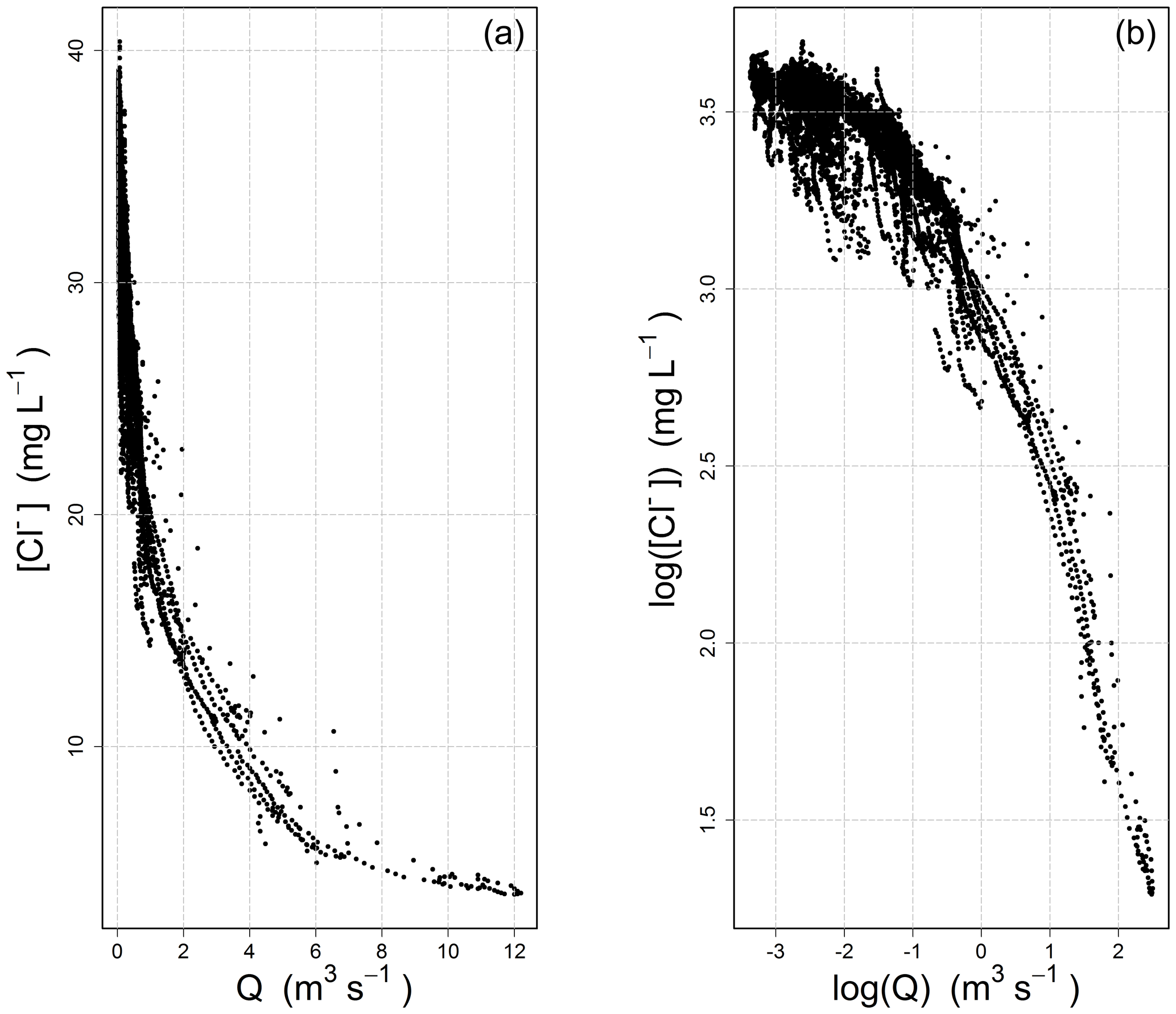
Figure 1 Concentration–discharge relationship observed at the Orgeval-ORACLE observatory (measurements from the River Lab) for chloride ions [Cl⁻]: (a) standard axes, (b) logarithmic axes.

Figure 1 illustrates the inadequateness of the power law for this dataset: the C-Q relationship evolves from a well-defined concave shape on the left to a slightly convex shape on the right in the log–log space. From the point of view of a modeler wishing to adjust a linear model, one has gone beyond the straight shape that was aimed at. Note that this is true for our dataset, and that it does not need to always be the case: the log–log space can be well adapted in some situations (see examples in the paper by Moatar et al., 2017).

3.3 A two-sided affine power scaling relationship as a progressive alternative to the power law

As a progressive alternative to the one-sided power scaling relationship (power law), we propose to use a two-sided affine power scaling (2S-APS) relationship as shown in Eq. (3) (Box and Cox, 1964; Howarth and Earle, 1979).

$$\begin{array}{}\text{(3)}& C^{\frac{\mathrm{1}}{n}}=a+b{Q}^{\frac{\mathrm{1}}{n}}\end{array}$$

From a numerical point of view, the relationship presented in Eq. (3) is equivalent to first transforming the dependent (C) and independent (Q) variables using a so-called Box–Cox transformation (Box and Cox, 1964), and then adjusting a linear model. In comparison with the logarithmic transformation, the additional degree of freedom offered by n allows for a range of transformations, from the untransformed variable (n=1) to the logarithmic transformation (n→∞). This “progressive” property was underlined long ago by Box and Cox (1964): when n takes high values, Eq. (3) converges toward the one-sided power scaling relationship (power law) (Eq. 1). The reason is simple:

$$C^{\frac{\mathrm{1}}{n}}=e^{\frac{\mathrm{1}}{n}\ln C}\approx \mathrm{1}+{\displaystyle \frac{\mathrm{1}}{n}}\ln C$$

when n is large.

Thus, for large values of n, Eq. (3) can be written as

$$\mathrm{1}+{\displaystyle \frac{\mathrm{1}}{n}}\ln C\approx a+b+{\displaystyle \frac{b}{n}}\ln Q.$$

That is equivalent to

$$\ln C\approx A+b\ln Q(\text{with }A=n(a+b-\mathrm{1}\left)\right).$$

The progressive behavior and the convergence toward the log–log space are clearly evident in Fig. 2.

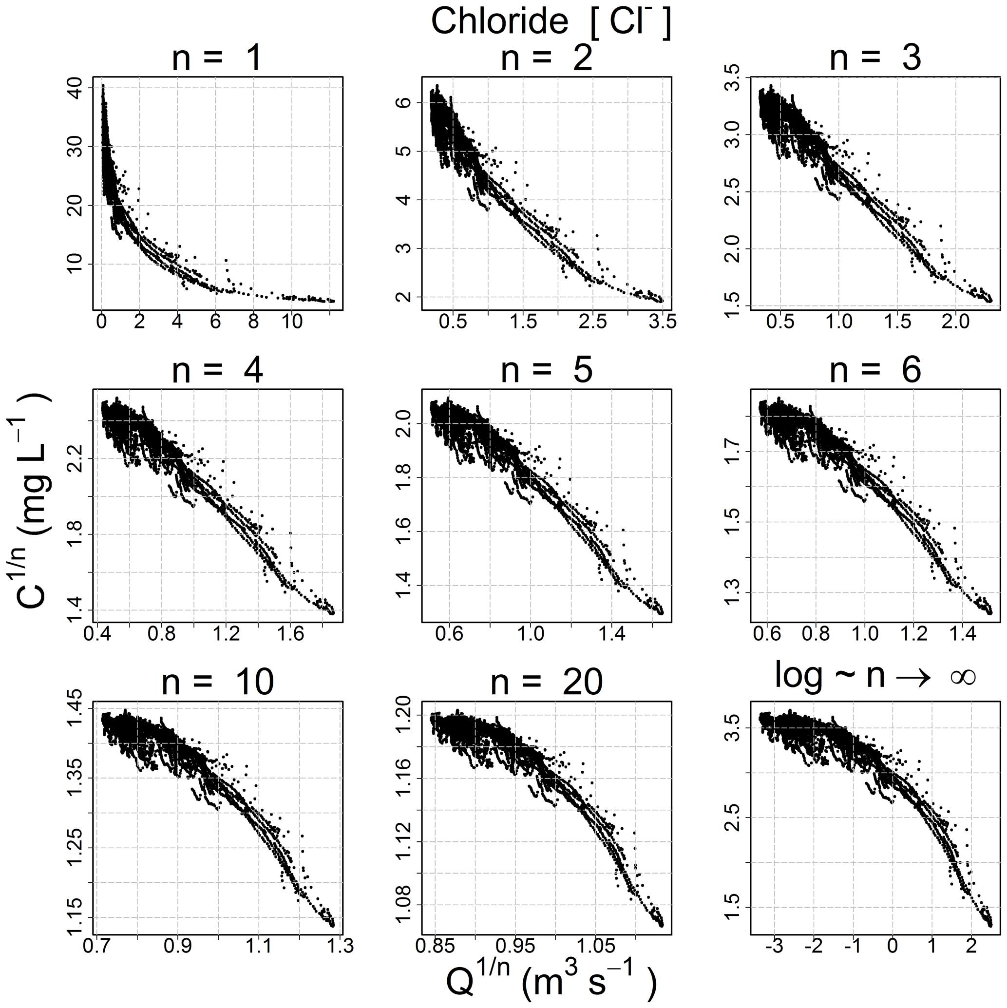
Figure 2 Evolution of the shape of the concentration–discharge scatterplot for chloride ion with two-sided affine power scaling (2S-APS) and an increasing value of parameter n.

3.4 Choosing an appropriate transformation for different ion species (calibration mode)

Because the hydro-biogeochemical processes that control the transport and reaction of ions are different, different ionic species may have a C–Q relationship of distinct shape (Moatar et al., 2017). In Fig. 3, we show the behavior of three ions and the EC from the same catchment and the same dataset (all four from the Orgeval-ORACLE observatory) with different transformations (n=1, 3, 5 and logarithmic transformation). The optimal shape was chosen numerically: we transformed our data series of C and Q using different values of n (i.e., $C^{\ast }=C^{\mathrm{1}/n}$ and $Q^{\ast }=Q^{\mathrm{1}/n}$) and logarithmic transformation (i.e., $C^{\ast \ast }=\log \left(C\right)$ and $Q^{\ast \ast }=\log \left(Q\right)$). With these transformed values, we performed a linear regression and computed parameter a and b and the coefficient of determination (R²) (see Table 2). The n considered as optimal has the highest R² value (see Table 2). However, we could also have followed the advice of Box et al. (2016, p. 331) and done it visually (Fig. 3).

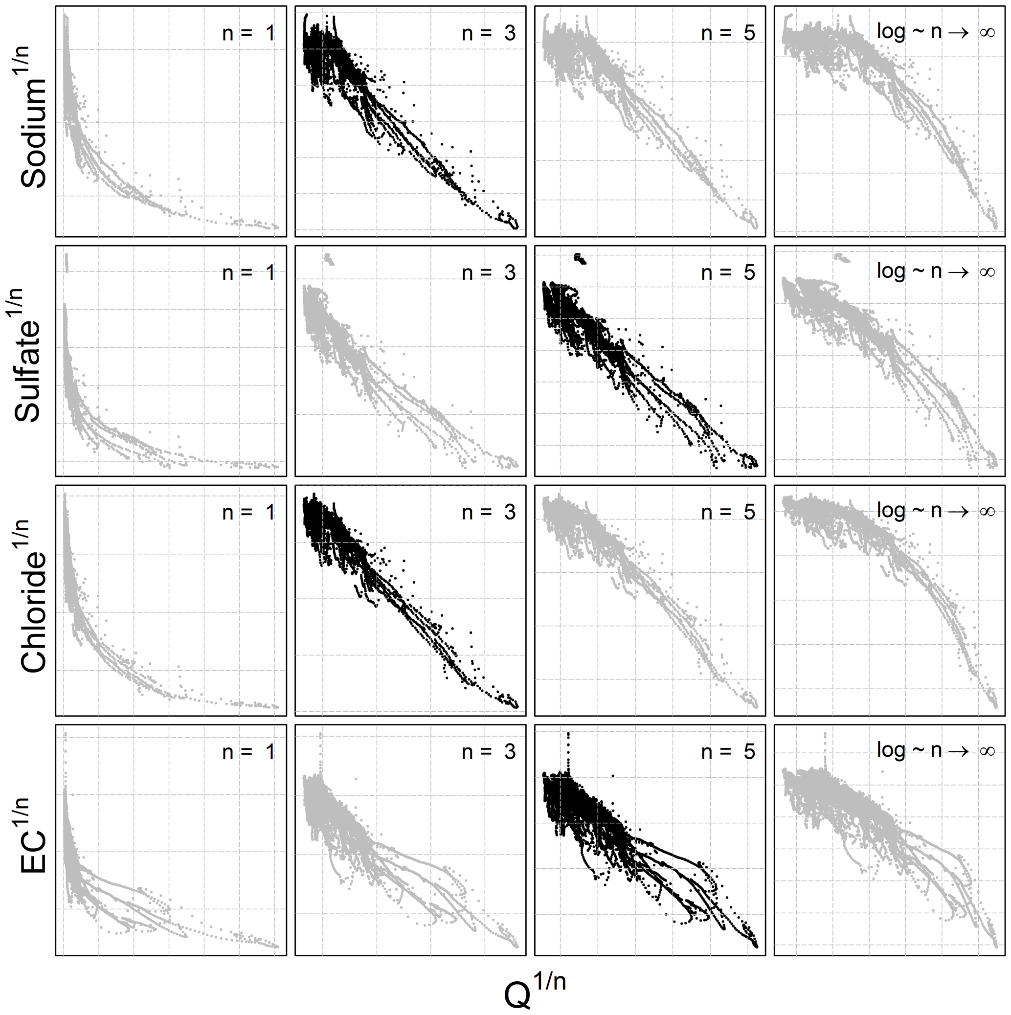
Figure 3 C–Q behavior of three different chemical species and the electrical conductivity with different 2S-APS transformations (n=1, 3, 5, and log). The optimal power parameter (black dots) was chosen based on the R² criterion. Note that we have removed the scale on the axes to focus only on the change in shape in the C–Q relationship.

Table 2 Coefficient of determination (R²) calculated for n=1 (no transformation), n= optimal value for two-sided affine power scaling relationship (Fig. 3) and n→∞ (log–log space) for each ion and for electrical conductivity (EC). Note that the R² is computed from transformed values.

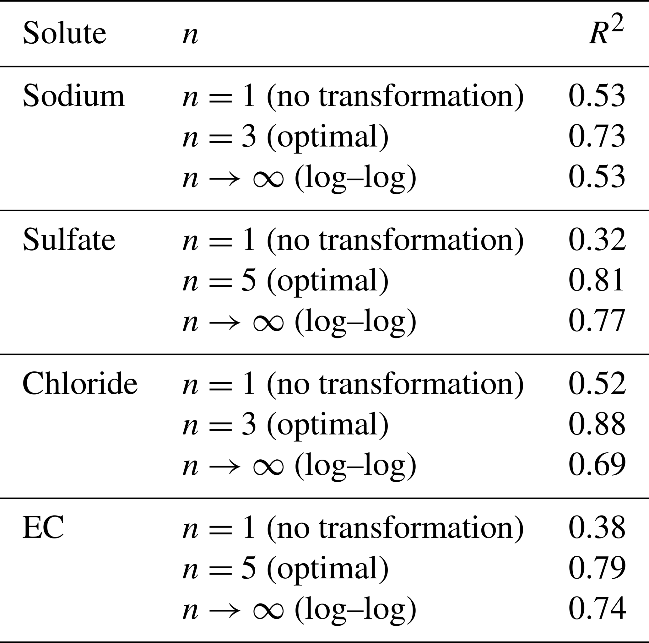
The results given in Table 2 show the better quality of the fit obtained with the optimal value of n.

4 Numerical identification of the parameters for the 2S-APS relationship

The extremely large number of values in this high-frequency dataset may cause problems for a robust identification over the full range of discharges using a simple linear regression. Indeed, the largest discharge values are in small numbers (in our dataset only 1 % of discharges are in the range [2.6, 12.2 m³ s⁻¹], and they correspond to the lowest concentrations; see Fig. 1).

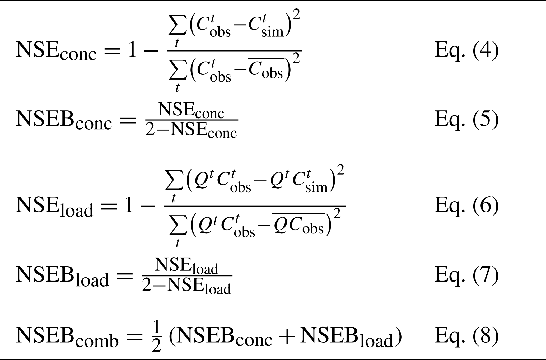
To address this question, we successively tested a large number of (a,b) pairs from Eq. (3) (n remaining fixed at the optimal value given in Table 2). Each pair yields a series of simulated concentrations (C_sim) that can be compared with the observed concentrations (C_obs). Among the many numerical criteria that could be used, we chose the bounded version of the Nash and Sutcliffe (1970) efficiency criterion NSEB (Mathevet et al., 2006), which is commonly used in hydrological modeling. NSEB can be computed on concentrations or on discharge-weighted concentrations (which corresponds to the load). We chose the average of both, because we found that it allows more weight to be given to the extremely low concentrations and thus to avoid the issue of under-representation of high-discharge/low-concentration measurement points. Table 3 presents the formula for these numerical criteria.

Table 3 Numerical criteria used for optimization (C_obs – observed concentration, C_sim – simulated concentration, Q – observed discharge). The Nash and Sutcliffe (1970) efficiency (NSE) criterion is well known and widely used in the field of hydrology. The rescaling proposed by Mathevet et al. (2006) transforms NSE into NSEB, which varies between −1 and 1 (its optimal value). The advantage of this rescaled version is to avoid the occurrence of large negative values (the original NSE criterion varies in the range [$-\mathrm{\infty },\mathrm{1}$]).

We retained as optimal the pair of (a,b) that yielded the highest NSEB_comb value (we explored in a systematic fashion the range [1–5] for a and [−1.2–1.2] for b).

In Appendix A2, we show that our proposed methodology for the identification of parameters a, b and n, based on the NSEB_comb criterion, is effective also from the point of view of the predictive confidence interval.

5 Results

5.1 Results in calibration mode

The optimal values of a and b corresponding to the simulation of each ion and EC with the highestNSEB_comb criterion and the n value identified in Fig. 3 and Table 2 are presented in Table 4.

Table 4 Summary of values a, b, and n used to obtain the optimal NSEB_comb criterion.

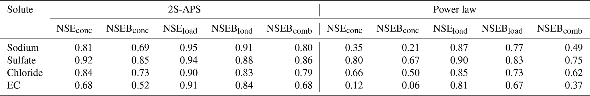
The five NSE criteria (defined in Table 3) used to identify the parameters of the 2S-APS relationship have also been computed for the power law relationship. The results are given in Table 5: the values obtained for the 2S-APS relationship are always higher than those calculated for the power law relationship.

Table 5 NSE criteria computed for the three ions and EC.

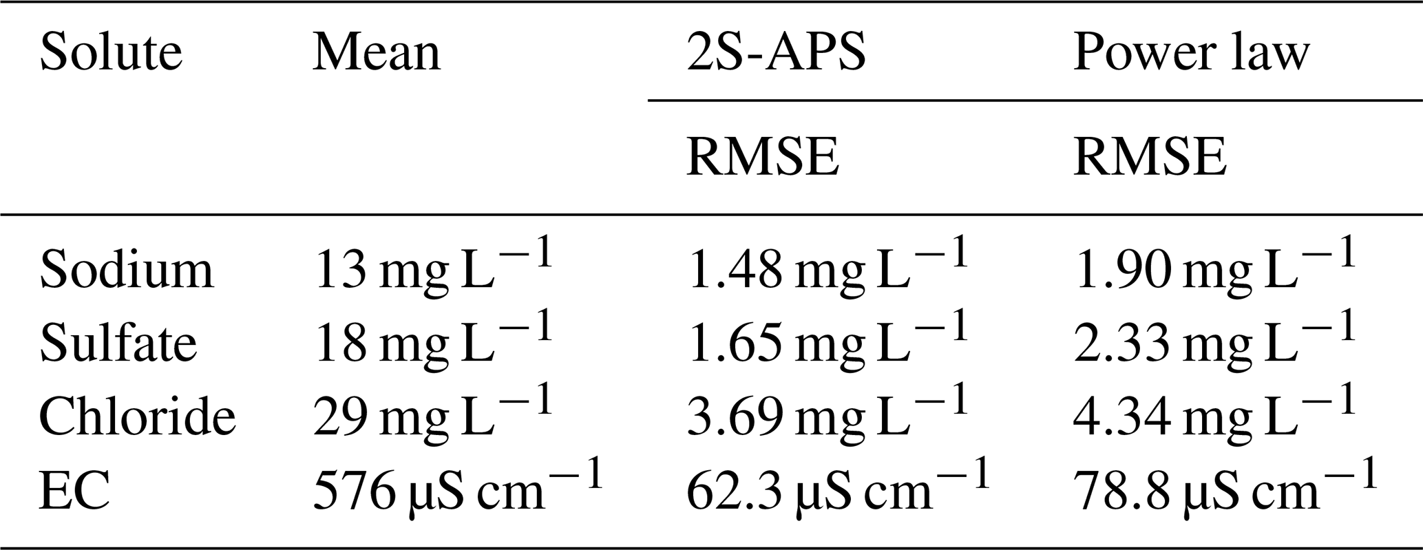
Also for comparing the two relationships, we used the RMSE criterion. The results are shown in Table 6; they illustrate (for our catchment) the better performance (i.e., lower RMSE value) of the proposed 2S-APS relationship for the three ions (sodium, sulfate, and chloride) over the power law relationship. For EC, there is a slight advantage over the power law. A test of the equality of variance (F test) was performed between the RMSE obtained for the two relationships: because of the very large number of points in our dataset, all differences were highly significant (p value <0.001).

Table 6 Summary of values of RMSE criterion calculated for the three ions and EC.

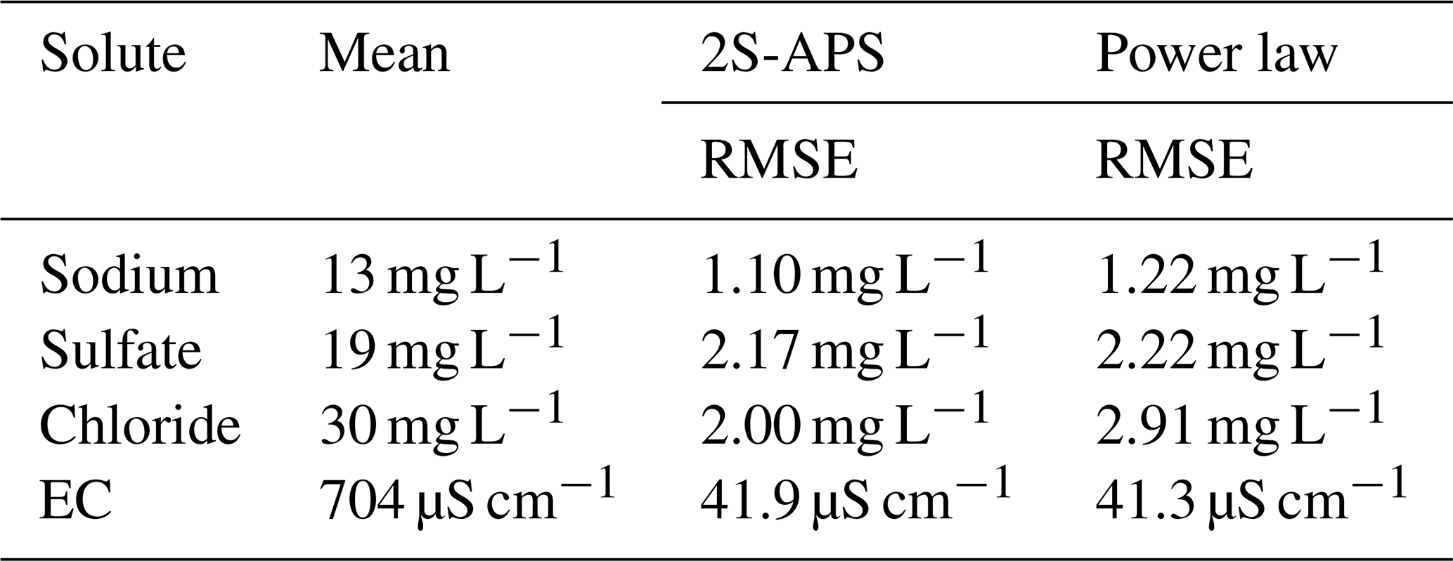
Figure 4 illustrates the comparison of the quality of simulation over the entire calibration dataset between the power law and 2S-APS relationships. In general, the two-sided affine power scaling relationship yields better simulated concentrations than the classic power law relationship for the two ions (according to the results of Table 6). This is particularly evident over the low concentrations (see Fig. 4). This better performance is more apparent in the case of sodium and chloride ions.

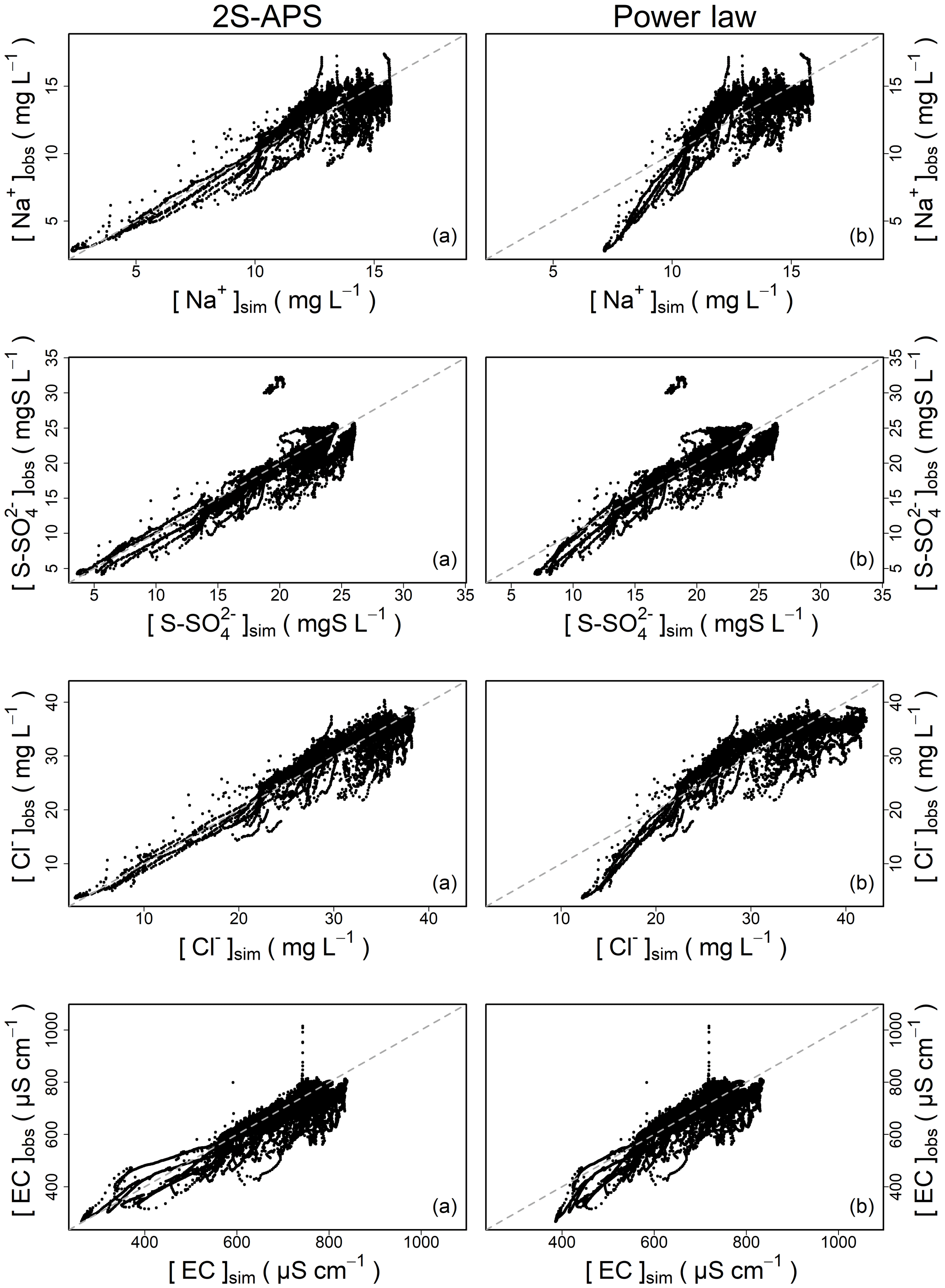
Figure 4 Comparison of simulated concentrations with observed concentrations for (a) two-sided affine power scaling (2S-APS) relationship, (b) power law (calibration mode).

5.2 Results in validation mode

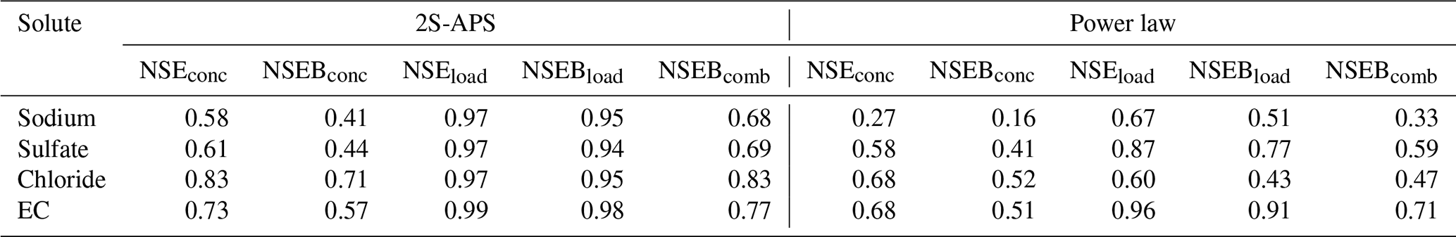
For the validation mode, we applied the above-calibrated relationships to a different time period (August 2017 to March 2018). We used as in Table 5 the five NSE criteria (see Table 3) to compare the performance between the two relationships studied. The results are given in Table 7. As in the calibration period, the values obtained for the 2S-APS relationship are higher than those calculated for the power law.

Table 7 NSE criteria computed for the three ions and EC.

Also, as in the calibration mode, we computed the RMSE criterion. The results are shown in Table 8. The RMSE criterion illustrates (for our catchment) the better performance of the proposed 2S-APS relationship over the power law relationship for all the solutes. Unlike the calibration case, the quality of the simulation of EC using the 2S-APS relationship has a much better performance than the one simulated by the power law relationship.

Table 8 Summary of values of RMSE criterion calculated for the three ions and EC with the validation dataset.

6 Conclusion

In this technical note, we tested and validated a three-parameter relationship (2S-APS) as an alternative to the classic two-parameter one-sided power scaling relationship (commonly known as “power law”), to represent the concentration–discharge relationship. We also proposed a way to calibrate the 2S-APS relationship.

Our results (in calibration and validation mode) show that the 2S-APS relationship can be a valid alternative to the power law: in our dataset, the concentrations simulated for sodium, sulfate, and chloride and the EC are significantly better in validation mode, with a reduction in RMSE ranging between 15 % and 26 %.

Naturally, because the data used for this study come from a single catchment, wider tests will be necessary to judge of the generality of our results.

Appendix A

A1 Description of the River Lab

In June 2015, the “River Lab” was deployed on the bank of the Avenelles River (within the limits of the Orgeval-ORACLE observatory, see Fig. A1) to measure the concentration of all major dissolved species at high frequency (Floury et al., 2017). The River Lab's concept is to “permanently” install a series of laboratory instruments in the field in a confined bungalow next to the river. River Lab performs a complete analysis every 30 min using two Dionex^® ICS-2100 ionic chromatography (IC) systems by continuous sampling and filtration of stream water. River Lab measures the concentration of all major dissolved species ([Mg²⁺], [K⁺], [Ca²⁺], [Na⁺], [Sr²⁺], [F⁻], [${\mathrm{SO}}_{\mathrm{4}}^{\mathrm{2}-}$] [${\mathrm{NO}}_{\mathrm{3}}^{-}$], [Cl⁻], [${\mathrm{PO}}_{\mathrm{4}}^{\mathrm{3}-}$]). In addition, a set of physico-chemical probes is deployed to measure pH, conductivity, dissolved O₂, dissolved organic carbon (DOC), turbidity, and temperature. The discharge is measured continuously via a gauging station located at the River Lab site.

All the technical qualities, calibration of the equipment, comparison with laboratory measurements, degree of accuracy, etc. have been well described in a publication by Floury et al. (2017).

A2 Predictive confidence interval (PI)

We have computed the predictive confidence interval, a well-known methodology used in linear regression (Jonnston, 1972, pp. 154–155; see also the discussion in Andréassian et al., 2007), to verify whether the 2S-APS relationship and the associated parameter identification methodology increase or decrease the uncertainty with respect to the power law relationship (linear regression with log transformation). We show two intervals: 50 % and 95 %. The results are given in Fig. A2: clearly, the predictive interval (blue surface for a 50 % predictive confidence interval, red for 95 %) is much narrower for the 2S-APS relationship than for the power law relationship. This can only reinforce our preference for the 2S-APS relationship.

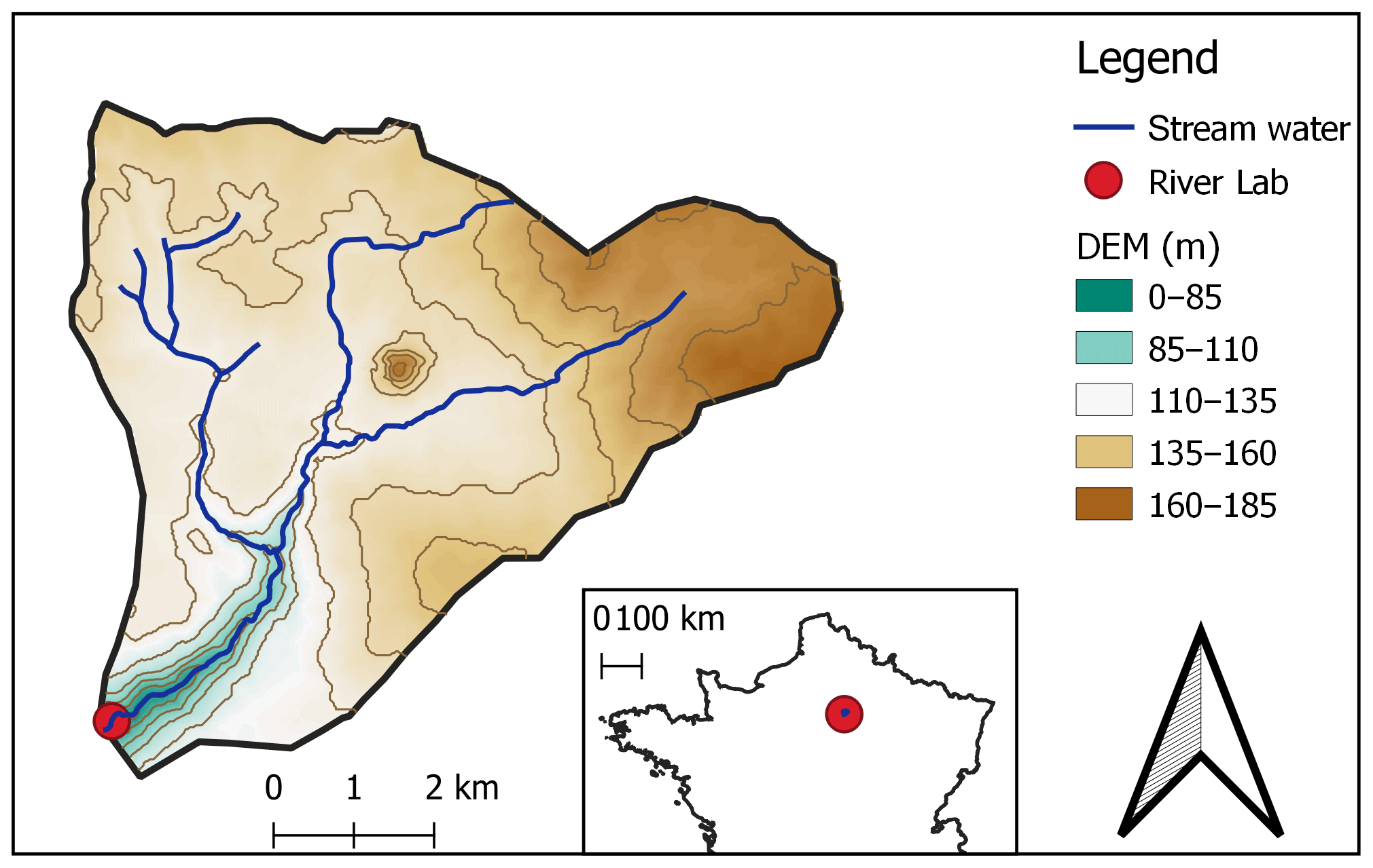
Figure A1 Location of the River Lab (red dot) on the Avenelles River, Orgeval-ORACLE observatory.

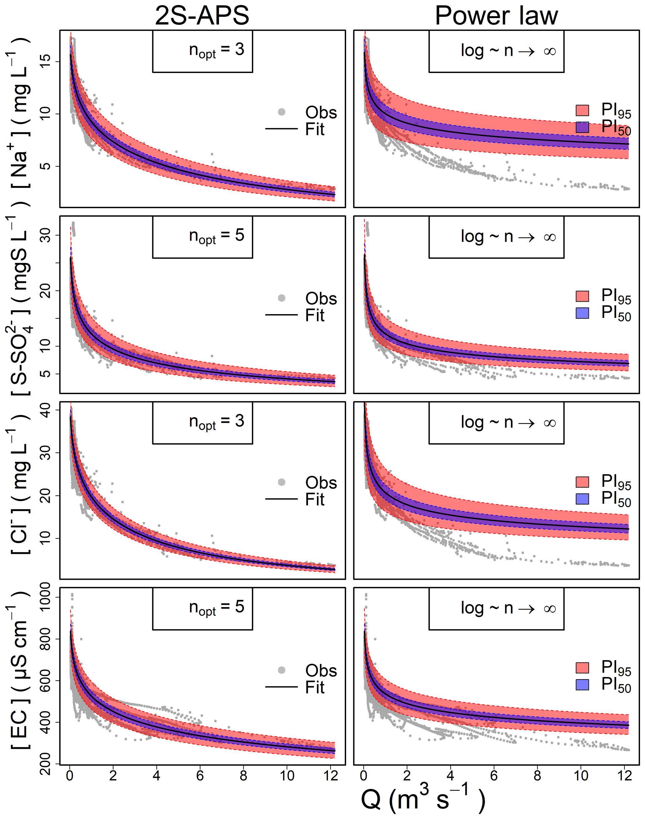
Figure A2 Predictive confidence interval computed for the 2S-APS relationship and the power law for the three ions and the EC relationship. In blue the 50 % and in red the 95 % predictive confidence intervals.