Flood trends in Europe: are changes in small and big floods different?

Recent studies have revealed evidence of trends in the median or mean flood discharge in Europe over the last 5 decades, with clear and coherent regional patterns. The aim of this study is to assess whether trends in flood discharges also occurred for larger return periods, accounting for the effect of catchment scale. We analyse 2370 flood discharge records, selected from a newly available pan-European flood database, with record length of at least 40 years over the period 1960–2010 and with contributing catchment area ranging from 5 to 100 000 km². To estimate regional flood trends, we use a non-stationary regional flood frequency approach consisting of a regional Gumbel distribution, whose median and growth factor can vary in time with different strengths for different catchment sizes. A Bayesian Markov chain Monte Carlo (MCMC) approach is used for parameter estimation. We quantify regional trends (and the related sample uncertainties), for floods of selected return periods and for selected catchment areas, across Europe and for three regions where coherent flood trends have been identified in previous studies. Results show that in northwestern Europe the trends in flood magnitude are generally positive. In small catchments (up to 100 km²), the 100-year flood increases more than the median flood, while the opposite is observed in medium and large catchments, where even some negative trends appear, especially in northwestern France. In southern Europe flood trends are generally negative. The 100-year flood decreases less than the median flood, and, in the small catchments, the median flood decreases less compared to the large catchments. In eastern Europe the regional trends are negative and do not depend on the return period, but catchment area plays a substantial role: the larger the catchment, the more negative the trend.

1 Introduction

Increasing flood hazard in Europe has become a major concern as a consequence of severe flood events experienced in the last decades, for instance the extreme floods that occurred in central Europe in 2002 (e.g. Ulbrich et al., 2003) and 2013 (e.g. Blöschl et al., 2013a), and the winter floods in northwest England in 2009 (e.g. Miller et al., 2013) and 2015/2016 (e.g. Barker et al., 2016). Hence a growing number of flood trend detection studies have been published in recent years. These studies typically analyse a large set of time series of flood peaks in a region and test them for the presence of significant gradual or abrupt changes in flood magnitude or frequency. For example, Petrow and Merz (2009) analysed eight flood indicators, from 145 gauges in Germany over the period 1951–2002, and detected mainly positive trends in the magnitude and frequency of floods. Villarini et al. (2011) tested flood time series of 55 stations in central Europe, with at least 75 years of data, for abrupt or gradual changes and found mostly abrupt changes associated with anthropogenic intervention (such as the construction of dams and reservoirs and river training). Mediero et al. (2014) detected a general decreasing trend in the magnitude and frequency of floods in Spain, with the exception of the northwest. Prosdocimi et al. (2014) investigated the presence of trends in annual and seasonal maxima of peak flows in the UK and found clusters of increasing trends for winter peaks in northern England and Scotland, and decreasing trends for summer peaks in southern England. These studies are highly heterogeneous in terms of flood data types, period of records and detection approaches, and it is therefore not trivial to deduce regional patterns of flood regime change at the larger continental scale. Despite this fragmentation, Hall et al. (2014) summarized the findings of previous studies in a map of increasing, decreasing and undetectable flood changes for Europe, and showed the existence of consistent regional patterns. In particular, in central and western Europe flood magnitude appeared to increase with time, while it seemed to decrease in the Mediterranean catchments and in eastern Europe.

More recently, thanks to the availability of European and global high-spatial-resolution databases, large-scale investigation studies across Europe have been published. Mangini et al. (2018) extracted 629 flood records from the Global Runoff Data Centre database (GRDC, 2016) and compared the detected trends in magnitude and frequency of floods from different approaches (annual maximum flood and peak over threshold) for the period 1965–2005. Blöschl et al. (2019) analysed 2370 flood records from a newly available pan-European flood database consisting of more than 7000 observational hydrometric stations and covering the last 5 decades (Hall et al., 2015) and revealed consistent spatial patterns of trends in the magnitude of the annual maximum flood, with clear positive trends in northwestern Europe and decreasing trends in southern and eastern Europe.

Existing studies typically analyse catchments individually and investigate whether spatial clusters or coherent regional patterns of flood trends can be observed (e.g. Petrow and Merz, 2009; Prosdocimi et al., 2014; Mangini et al., 2018). Based on predefined regions or obtained change patterns, some studies aggregate flood records and local test results in order to assess their field significance (e.g. Douglas et al., 2000; Mediero et al., 2014; Renard et al., 2008). The main limitation of most at-site studies is the short length of the flood peak records locally available for the detection of trends, resulting in low signal-to-noise ratio and hence high uncertainties in the detected trend. Increasing the signal-to-noise ratio can be achieved by pooling flood data from multiple sites within homogeneous regions, as in regional frequency analyses (Dalrymple, 1960; Hosking and Wallis, 1997). Several studies propose non-stationary regional frequency analyses for changes in precipitation extremes and flood trends that consider the dependency of regional estimates on time (e.g. Cunderlik and Burn, 2003; Renard et al., 2006a; Leclerc and Ouarda, 2007; Hanel et al., 2009; Roth et al., 2012) or on climatic and anthropogenic covariates (e.g. Lima and Lall, 2010; Tramblay et al., 2013; Renard and Lall, 2014; Sun et al., 2014; Prosdocimi et al., 2015; Viglione et al., 2016). Other approaches analyse coherent regional change by testing for the presence of trends in regional variables, as the number of annual floods in the region (e.g. Hannaford et al., 2013), or with regional tests (e.g. Douglas et al., 2000; Renard et al., 2008).

However, most of the cited studies investigate changes in the mean annual (or median) flood only, and few examples exist where observed trends in different flood quantiles are analysed. Typically, flood quantiles obtained with stationary and non-stationary flood frequency approaches are compared (see e.g. Machado et al., 2015; Šraj et al., 2016; Silva et al., 2017). The detection of changes in the magnitude of flood quantiles is much more common for precipitation (e.g. Hanel et al., 2009) or in flood projection studies (e.g. Prudhomme et al., 2003; Leander et al., 2008; Rojas et al., 2012; Alfieri et al., 2015).

To address this research gap, the aim of this study is to assess the changes in small vs. big flood events (corresponding to selected flood quantiles) across Europe over 5 decades (i.e. 1960–2010), and to determine whether these changes have been subject to different degrees of modification in time. Moreover, given that the impacts of different drivers of change on floods are expected to be strongly dependent on spatial scales (Blöschl et al., 2007; Hall et al., 2014), it is also of interest to assess the effect of catchment area, by comparing changes of flood quantiles for catchments of different sizes. Since the length of at-site flood records is often not sufficient to enable the reliable estimation of flood quantiles associated with high return periods (i.e. low probability of exceedance, e.g. the 100-year flood), in this study we adopt a (non-stationary) regional flood frequency approach, which pools flood data of multiple sites in order to increase the robustness of the estimated regional flood frequency curve and its changes over time. The methods and the flood database are described in detail in Sect. 2. The results are presented in Sect. 3, where we show the estimation of the flood quantiles and their trends in one example region (Sect. 3.1), the patterns of flood regime changes emerging from a spatial moving-window analysis across Europe (Sect. 3.2) and the flood regime changes in three relevant macro-regions (Sect. 3.3).

2 Methods

2.1 Regional flood change model

In order to quantify the changes in time in flood quantiles corresponding to different return periods for catchments of different size, we propose a regional flood change model that is more robust than local (at-site) trend analysis, in particular regarding trends associated with large quantiles of the flood frequency curve. We assume annual maximum flood peak discharges to follow the Gumbel distribution (i.e. extreme-value distribution type I), whose cumulative distribution is defined as

$$F_X\left(x\right)=p=\exp \left(-\exp \left(-{\displaystyle \frac{x-\mathit{\xi }}{\mathit{\sigma }}}\right)\right)=\exp \left(-\exp \left(-y\right)\right),$$

where ξ and σ are the location and scale parameter and

$$y={\displaystyle \frac{x-\mathit{\xi }}{\mathit{\sigma }}}=-\ln (-\ln p)$$

is the Gumbel reduced variate. The corresponding quantile function, i.e. the inverse of the cumulative distribution function, is

$$q\left(p\right)=\mathit{\xi }-\mathit{\sigma }\ln \left(-\ln p\right)=\mathit{\xi }+\mathit{\sigma }y.$$

In this paper we consider two alternative parameters which better relate to the literature on regional frequency analysis, especially to the index flood method of Dalrymple (1960) and Hosking and Wallis (1997). The alternative parameters are (1) the 2-year quantile or median q₂ (which corresponds to the index flood) and (2) the 100-year growth factor $x_{\mathrm{100}}^{\prime }$, which gives the 100-year quantile as $q_{\mathrm{100}}=q_{\mathrm{2}}(\mathrm{1}+x_{\mathrm{100}}^{\prime })$ in a similar fashion to the modified quantiles in Coles and Tawn (1996) and Renard et al. (2006b). The relationships linking these alternative parameters to the Gumbel location and scale parameters are

$$\begin{array}{ll}{\displaystyle }& {\displaystyle }{q}_{\mathrm{2}}=\mathit{\xi }+\mathit{\sigma }{y}_{\mathrm{2}},\\ {\displaystyle }& {\displaystyle }{x}_{\mathrm{100}}^{\prime }=\mathit{\sigma }(y_{\mathrm{100}}-y_{\mathrm{2}})/(\mathit{\xi }+\mathit{\sigma }{y}_{\mathrm{2}}),\end{array}$$

where $y_{\mathrm{2}}=-\ln (-\ln (\mathrm{0.5}\left)\right)$ and $(y_{\mathrm{100}}-y_{\mathrm{2}})=-\ln (-\ln (\mathrm{0.99}\left)\right)+\ln (-\ln (\mathrm{0.5}\left)\right)$. The quantile function, with the alternative parametrization, is here expressed as a function of the return period $T=\mathrm{1}/(\mathrm{1}-p)$ as

$$\begin{array}{}\text{(1)}& q_{\mathrm{T}}=q_{\mathrm{2}}\left(\mathrm{1}+a_T{x}_{\mathrm{100}}^{\prime }\right),\end{array}$$

where $a_T=(y_T-y_{\mathrm{2}})/(y_{\mathrm{100}}-y_{\mathrm{2}})$ and $y_T=-\ln (-\ln (\mathrm{1}-\mathrm{1}/T\left)\right)$. In particular, a_T=0 for T=2 and a_T=1 for T=100.

In the following we estimate the parameters of the Gumbel distribution both locally and regionally. For the local case, we allow the parameters to change with time according to the following log–linear relationships:

$$\begin{array}{ll}{\displaystyle }& {\displaystyle }\ln q_{\mathrm{2}}=\ln {\mathit{\alpha }}_{{\mathrm{2}}_{\mathrm{0}}}+{\mathit{\alpha }}_{{\mathrm{2}}_{\mathrm{1}}}\cdot t,\\ \text{(2)}& {\displaystyle }& {\displaystyle }{\displaystyle }& {\displaystyle }\ln x_{\mathrm{100}}^{\prime }=\ln {\mathit{\alpha }}_{g_{\mathrm{0}}}+{\mathit{\alpha }}_{g_{\mathrm{1}}}\cdot t.\end{array}$$

For the regional case we introduce the scaling of q₂ and $x_{\mathrm{100}}^{\prime }$ with catchment area S, according to the following relationships:

$$\begin{array}{ll}{\displaystyle }& {\displaystyle }\ln q_{\mathrm{2}}=\ln {\mathit{\alpha }}_{{\mathrm{2}}_{\mathrm{0}}}+{\mathit{\gamma }}_{{\mathrm{2}}_{\mathrm{0}}}\ln S+({\mathit{\alpha }}_{{\mathrm{2}}_{\mathrm{1}}}+{\mathit{\gamma }}_{{\mathrm{2}}_{\mathrm{1}}}\ln S)\cdot t+\mathit{\epsilon },\\ \text{(3)}& {\displaystyle }& {\displaystyle }\ln x_{\mathrm{100}}^{\prime }=\ln {\mathit{\alpha }}_{g_{\mathrm{0}}}+{\mathit{\gamma }}_{g_{\mathrm{0}}}\ln S+({\mathit{\alpha }}_{g_{\mathrm{1}}}+{\mathit{\gamma }}_{g_{\mathrm{1}}}\ln S)\cdot t,{\displaystyle }& {\displaystyle }\mathit{\epsilon }\sim \mathcal{N}\left(\mathrm{0},\mathit{\sigma }\right),\end{array}$$

where the α and γ terms are parameters to be estimated (the γ terms control the scaling with area) and the ε term accounts for the fact that additional local variability, on top of the one explained by time and catchment area, is affecting the index flood but not the growth curve. In our model, a homogeneous region is thus formed by sites whose growth curve depends on catchment area and time only, and whose index flood also depends on other factors which determine additional noise (here assumed normal).

We investigate changes in flood quantiles associated with fixed annual exceedance probability 1−p or, equivalently, with fixed return period $T=\mathrm{1}/(\mathrm{1}-p)$. The relative change in time of the generic flood quantile q_T is thus derived, for the local case, from Eqs. (1) and (2) as

$$\begin{array}{}\text{(4)}& {\displaystyle \frac{\mathrm{1}}{q_{\mathrm{T}}}}{\displaystyle \frac{\mathrm{d}{q}_{\mathrm{T}}}{\mathrm{d}t}}={\mathit{\alpha }}_{{\mathrm{2}}_{\mathrm{1}}}+{\mathit{\alpha }}_{g_{\mathrm{1}}}-{\displaystyle \frac{{\mathit{\alpha }}_{g_{\mathrm{1}}}}{\mathrm{1}+a_T{x}_{\mathrm{100}}^{\prime }}}\end{array}$$

and, for the regional case, from Eqs. (1) and (3) as

$$\begin{array}{}\text{(5)}& {\displaystyle \frac{\mathrm{1}}{q_{\mathrm{T}}}}{\displaystyle \frac{\mathrm{d}{q}_{\mathrm{T}}}{\mathrm{d}t}}={\mathit{\alpha }}_{{\mathrm{2}}_{\mathrm{1}}}+{\mathit{\alpha }}_{g_{\mathrm{1}}}+({\mathit{\gamma }}_{{\mathrm{2}}_{\mathrm{1}}}+{\mathit{\gamma }}_{g_{\mathrm{1}}})\ln S-{\displaystyle \frac{{\mathit{\alpha }}_{g_{\mathrm{1}}}+{\mathit{\gamma }}_{g_{\mathrm{1}}}\ln S}{\mathrm{1}+a_T{x}_{\mathrm{100}}^{\prime }}}.\end{array}$$

The model parameters, the quantiles and their local and regional relative trends are estimated by fitting the local and regional models to flood data with Bayesian inference through a Markov chain Monte Carlo (MCMC) approach. One of the advantages of the Bayesian MCMC approach is that the credible bounds of the distribution parameters (and other estimated quantities) can be directly obtained from their posterior distribution, without any additional assumption. The MCMC inference is performed using the R package rStan (Carpenter et al., 2017). It generates samples with a Hamiltonian Monte Carlo algorithm that uses the derivatives of the density function being sampled to generate efficient transitions spanning the posterior (Stan Development Team, 2018). For each inference, four chains, with 100 000 simulations each, are generated with different initial values of the parameters and checked for their convergence. An improper uniform prior distribution over the entire real line is set for the parameters, with the exception of ${\mathit{\alpha }}_{{\mathrm{2}}_{\mathrm{0}}}$ and ${\mathit{\alpha }}_{g_{\mathrm{0}}}$, for which we use an improper uniform prior distribution over the entire positive real line. When fitting the regional model, we make the assumption of regional homogeneity with regards to the distribution of flood peaks, allowing local variability of the median value and its changes in time.

Spatial cross-correlation between flood time series at different sites is not accounted for in this model (i.e. it assumes independence of flood time series in space); however, it is possible to quantify its effects in first approximation in a Bayesian framework through an approach based on a magnitude adjustment to the likelihood (Ribatet et al., 2012). This approach consists in scaling the likelihood with a proper constant exponent to be estimated between 0 and 1, which results in inflating the posterior variance of the parameters and consequent increase of the width of parameter uncertainty intervals, reflecting the overall effect of spatial dependence in the data. In the case of spatial independence the magnitude adjustment factor is 1, whereas values of the magnitude adjustment factor close to 0 indicate strong inter-site correlation of floods and substantially larger sample uncertainties resulting from the adjusted model compared to the model where spatial cross-correlation is not accounted for. For further details about the method and its application to hydrological data, see Smith (1990), Ribatet et al. (2012) and Sharkey and Winter (2019). We apply this method to an example region in central Europe, in order to quantify the magnitude of the uncertainty underestimation associated with the model assumption of spatial independence in flood data.

2.2 European flood database

In this study, we analyse annual maximum discharge series from a newly available pan-European flood database, consisting of more than 7000 observational hydrometric stations and covering 5 decades (Hall et al., 2015). Their contributing catchment areas range from 5 to 100 000 km², and several nested catchments are included in the database.

For comparability with Blöschl et al. (2019), only the stations satisfying the following selection criteria, based on record length and even spatial distribution, are considered for the estimation of the regional trends. We select stations with at least 40 years of data in the period 1960–2010, with the record starting in 1968 or earlier and ending in 2002 or later. Additionally, in order to ensure a more even spatial distribution across Europe, in Austria, Germany and Switzerland (countries with the highest density of stations in the database) the minimum record length accepted is 49 years; in Cyprus, Italy and Turkey a length of 30 years is accepted; and in Spain 40 years is accepted without restrictions to the start and end of the record. Figure 1 shows the locations of the 2370 stations satisfying the above selection criteria. The flood discharge data are accessible at https://github.com/tuwhydro/europe_floods (last access: 18 November 2019).

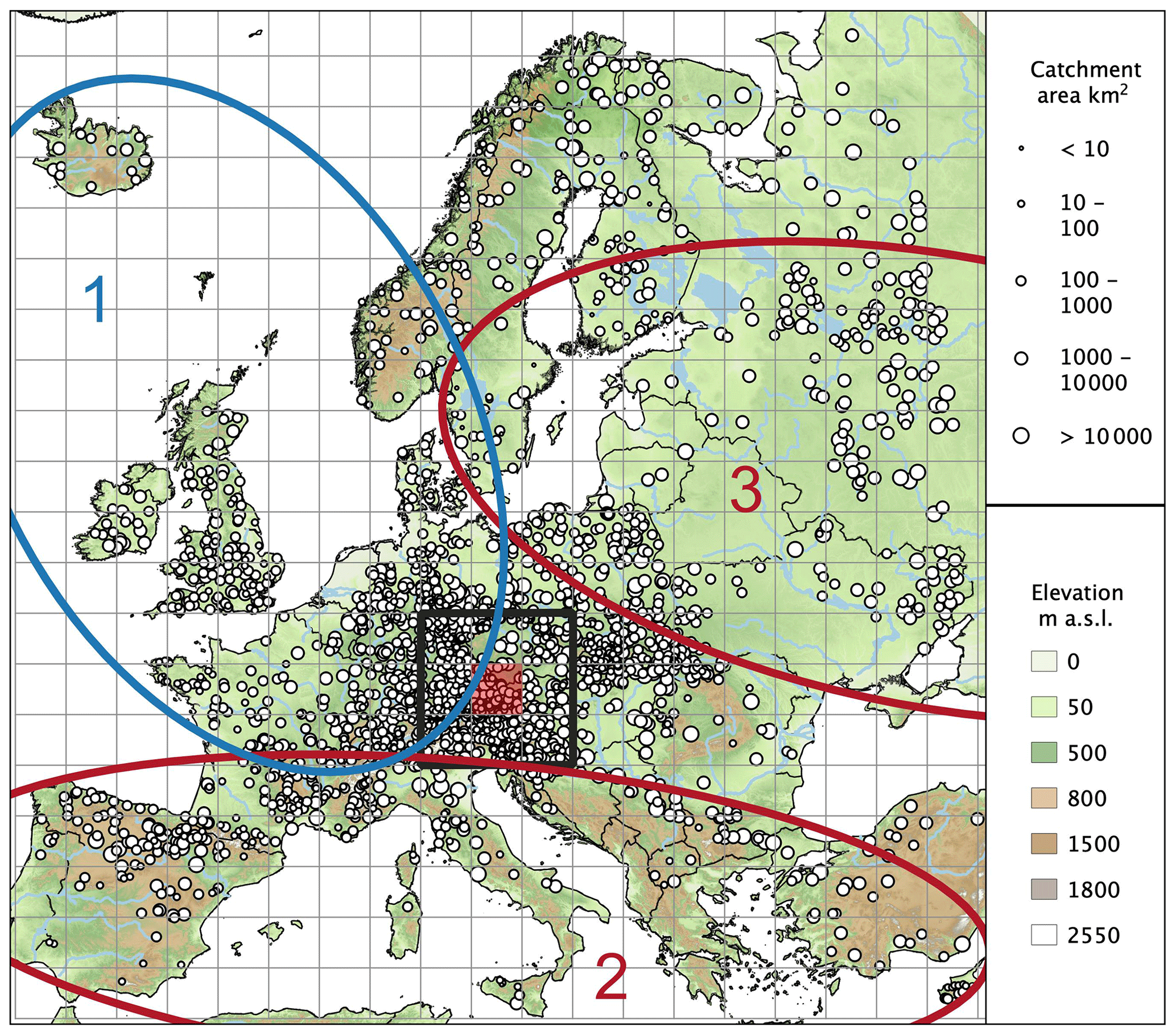
Figure 1 Location of the selected 2370 hydrometric stations in Europe and regions considered in this study. The size of the circles is representative for the contributing catchment area. The size of the grid cells is 200 km × 200 km. The black rectangle shows the size of the spatial moving windows analysed in Sect. 3.2. It consists of nine cells, corresponding to 600 km × 600 km. The three ellipses (numbers 1–3) mark homogeneous macro-regions, analysed in Sect. 3.3, and consist of (1) northwestern Europe, (2) southern Europe and (3) eastern Europe.

2.3 Experimental design for the regional analyses

In this study, the regional flood change model of Sect. 2.1 is initially fitted to flood data of multiple sites that are pooled within spatial windows with a size of 600 km × 600 km, with an overlapping length of 200 km in both directions. The size and overlapping length of the windows are chosen, after several preliminary tests, in order to ensure a sufficient number of gauges within each window and an appropriate spatial resolution at which to present the regional trends at the continental scale. Significant differences in spatial change pattern are not observed when changing the window size (not shown). The rationale behind the homogeneity assumption is that the spatial windows, given their size, are characterized by comparatively homogeneous climatic conditions (and hence flood generation processes) and processes driving flood changes. Figure 1 shows the resulting 200 km × 200 km grid cells. Each of the 600 km × 600 km windows considered in this analysis is composed of nine neighbouring cells as represented, for example, by the black rectangular region, whose regional trend estimates are shown in detail in Sect. 3.1. The example region is selected in central Europe because of the number of available gauges with different ranges of contributing catchment areas. In each window we estimate the regional relative trend in time of q₂ and q₁₀₀, as defined in Eq. (5), for small and big catchment sizes (i.e. assuming S=100 and 10 000 km² in the model). Note that this analysis intends to show the estimated flood trends in hypothetical catchments with a specific size, which do not exist everywhere across Europe, based on fitting the model to existing catchments. We plot the resulting trends on a map by assigning their values to the respective central 200 km × 200 km cell (e.g. the light red area in Fig. 1). The number of stations within each of the considered 600 km × 600 km windows is shown in Fig. A1 for several ranges of catchment size.

Figure 1 shows three macro-regions (numbers 1–3) located in northwestern Europe, southern Europe and eastern Europe, respectively. These regions were identified in Blöschl et al. (2019) by visual inspection of the flood trend and flood seasonality patterns and represent large homogeneous regions in terms of changes in the mean annual flood discharges. According to Köppen–Geiger climate classification (Köppen, 1884), northwestern Europe (region 1) corresponds approximately to the temperate oceanic climate zone, in southern Europe (regions 2) the hot- and warm-summer Mediterranean climate zones prevail, and eastern Europe (region 3) is dominated by warm-summer humid continental climate. Table 1 shows some related regional summary statistics. In this study, the same regions are analysed in terms of changes in flood quantiles, to allow a more detailed assessment of existing research and to allow for ready comparability of the results. The regional change model is consequently fitted to the pooled flood data of the sites within each of the three regions, and trends in small and big floods for small to large catchments are analysed (Sect. 3.3).

In summary, the following regional analyses are carried out:

• In Sect. 3.1 regional flood regime changes in central Europe are investigated. As an example, the regional model is fitted to the black rectangular region of Fig. 1, which contains 601 hydrometric stations. For this example region, the regional model flood quantiles and their trends in time are shown as a function of catchment area and of return period (as defined in Eqs. 1 and 5, respectively). The regional trends in q₂ and q₁₀₀ are compared for five hypothetical catchment sizes (S=10, 100, 1000, 10 000 and 100 000 km²), and local trend estimates (as in Eq. 4) are shown together with the regional trends. In this example region we also investigate the overall effect of spatial dependence in flood data on the width of the estimated credible bounds, with the approach based on the magnitude adjustment to the likelihood.

• In Sect. 3.2 regional flood regime changes across Europe are investigated. The regional model is fitted to overlapping windows across Europe, with a size of 600 km × 600 km, and the regional trends in q₂ and q₁₀₀ are estimated for small and big hypothetical catchments (S=100 and 10 000 km², respectively). Maps of the estimated trends are shown, where the trend values are plotted in the respective central 200 km × 200 km cell of each region. Differences among the estimated trends across Europe are calculated for further comparison.

• In Sect. 3.3 regional flood regime changes are investigated in three macro-regions, i.e. (1) northwestern Europe, (2) southern Europe and (3) eastern Europe. The regional model is fitted to these regions, and the regional trends in q₂ and q₁₀₀ are estimated and compared for five hypothetical catchment sizes (S=10, 100, 1000, 10 000 and 100 000 km²).

Table 1 Regional summary statistics (number of stations, mean catchment area, mean outlet elevation, mean record length) of the flood database for the considered macro-regions (1–3 in Fig. 1) and for Europe.

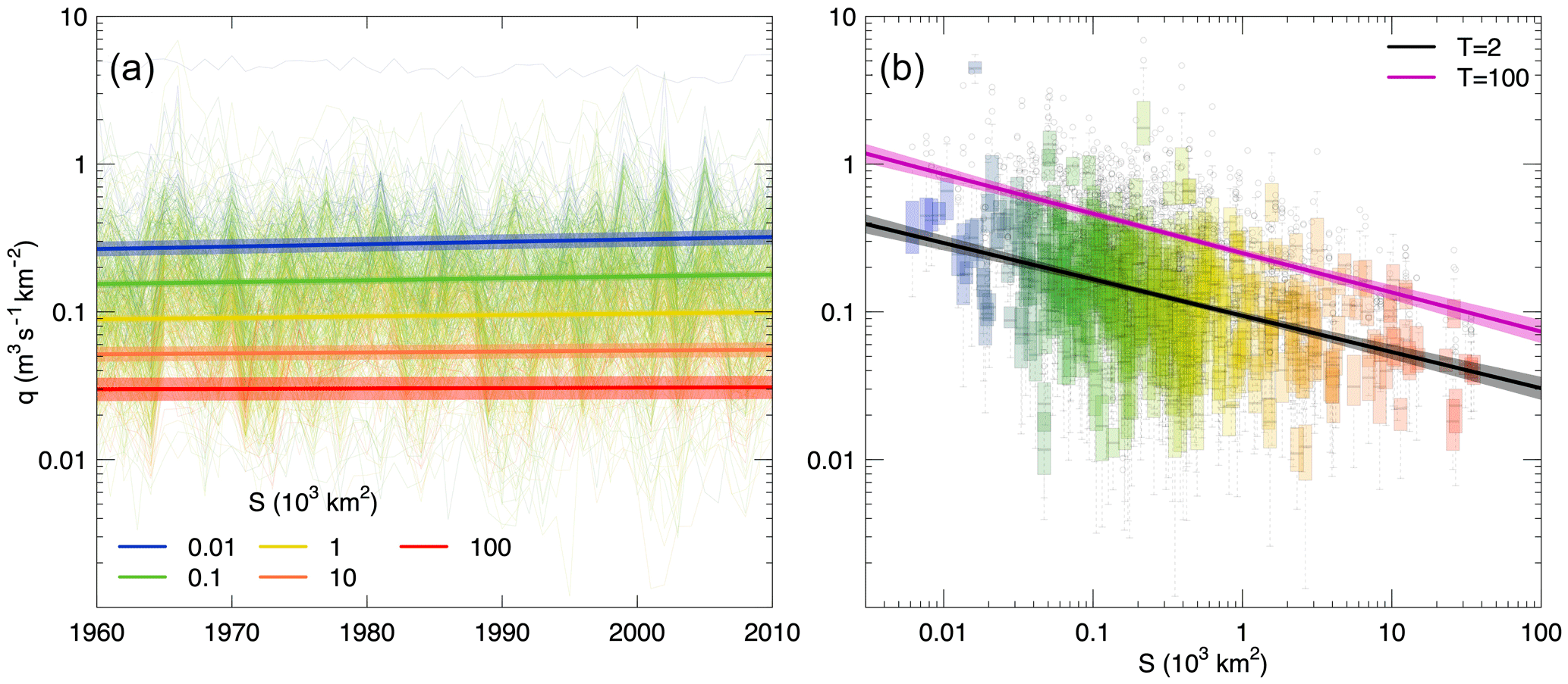
Figure 2 Fitting the regional model to flood data of 601 hydrometric stations in central Europe. In panel (a), annual maximum discharge series are shown with thin lines, with colours referring to catchment area. The thick lines and the shaded areas represent respectively the median and the 90 % credible intervals of the posterior distribution of the 2-year flood, for five hypothetical catchment areas (S=10, 100, 1000, 10 000 and 100 000 km², indicated by different colours). In panel (b), the box plots represent flood data as a function of catchment area. The thick lines and the shaded areas represent respectively the median and the 90 % credible intervals of the posterior distribution of flood quantiles, corresponding to return periods of 2 and 100 years. The curves are shown for 1985, i.e. the median year of the period analysed.

3 Results

3.1 Regional flood regime changes in central Europe

In this section, we show a detailed example of the (local and) regional model estimates for the black rectangular 600 km × 600 km window of Fig. 1, located in central Europe and containing 601 hydrometric stations. The annual maximum discharge series of these stations are shown in Fig. 2 (with thin lines and box plots in Fig. 2a and b, respectively). In the same figure, the regional flood quantiles q₂ (Fig. 2a and b) and q₁₀₀ (Fig. 2b), estimated with Eq. (1), are shown (thick lines and shaded areas) as a function of time for five selected catchment areas (S=10, 100, 1000, 10 000 and 100 000 km², indicated by different colours), in Fig. 2a, and as a function of catchment area for 1985 (i.e. the median year of the analysis period), in Fig. 2b. In both panels, the 90 % credible bounds (shaded areas) are shown together with the median (thick lines) of the posterior distribution of the regional flood quantiles. In general, both q₂ and q₁₀₀ (not shown) increase with time, and their trend is larger for smaller catchment areas. The uncertainties in the quantile estimates also vary with catchment area: for very small (e.g. 10 km²) and very large (e.g. 100 000 km²) catchments the credible bounds get larger, reflecting the scarcity of samples with these (extremely small and extremely large) sizes in the considered region (Fig. 1).

The two panels of Fig. 3 show the relative change in time, in per cent per decade, of the regional flood quantile estimates q_T (as defined in Eq. 5) as a function of catchment area and of the return period, respectively. The curves are shown for 1985, the median year of the analysed period. The trends in q_T are mostly positive, and their values tend to decrease with increasing catchment area, approaching zero and moving towards negative values for higher return periods and for very large catchment areas (S=100 000 km²). For small catchment areas (S < 100 km²) the trend tends to be bigger for floods with large return periods (q₁₀₀) than for small return periods (q₂). The opposite is observed for larger catchments. As in Fig. 2, we observe larger 90 % credible bounds of the quantile estimates for very small and very large catchment areas. In this case, the overall effect of spatial cross-correlation between flood time series at different sites is investigated through the magnitude adjustment to the likelihood. The credible bounds for the regional trends obtained with the likelihood adjustment (dashed lines in Fig. 3) are 17.6 to 23.8 % larger compared to the case where spatial cross-correlation is not accounted for (estimated magnitude adjustment factor 0.669).

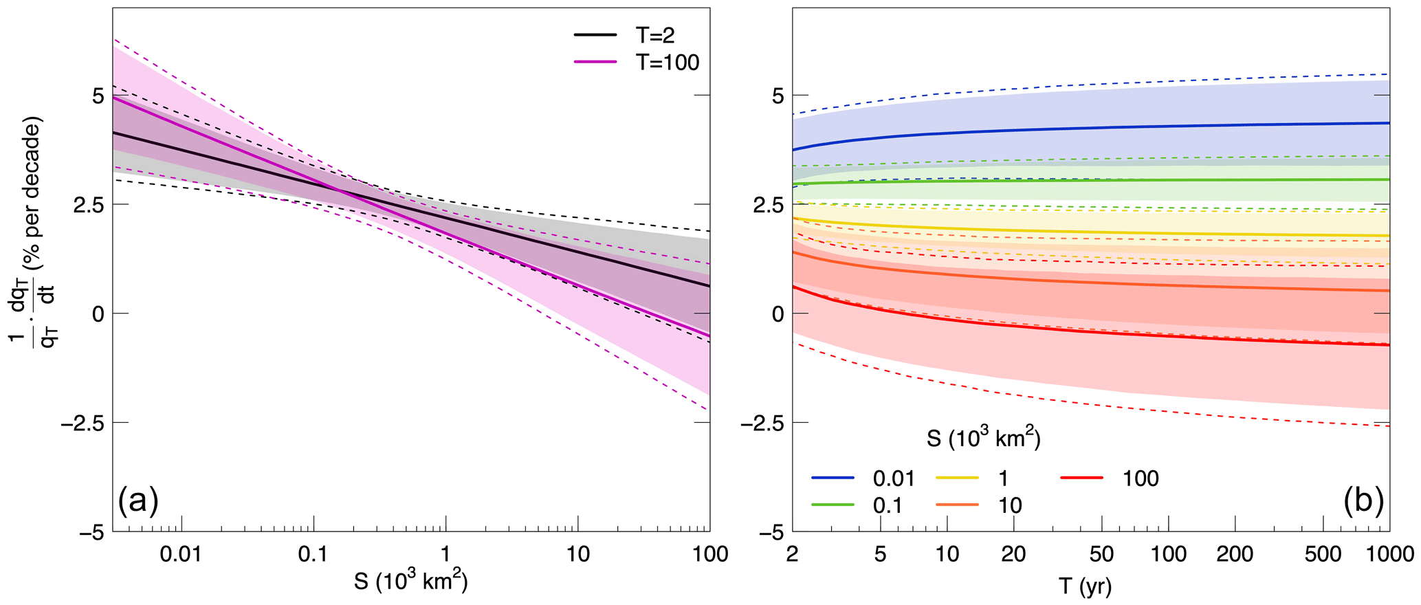
Figure 3 Estimates of the regional relative trend of q_T in per cent per decade as a function of catchment area and return period in central Europe. The thick solid lines and the shaded areas represent respectively the median and the 90 % credible intervals of the posterior distribution of the regional trends. Panel (a) shows the trend as a function of catchment area for selected values of the return period (T=2 and 100 years). Panel (b) shows the trend as a function of return period for five hypothetical catchment areas (S=10, 100, 1000, 10 000 and 100 000 km²). The curves are shown for the median year of the period analysed (i.e. 1985). The credible bounds obtained with the magnitude adjustment to the likelihood are shown with dashed lines.

Figure 4 Local and regional relative trend in per cent per decade in large (q₁₀₀) vs. small floods (q₂) in central Europe. Panel (a) shows the median of the posterior distribution of the local trends in q₁₀₀ vs. q₂ (light transparent dots in the background), with the respective 90 % credible intervals (error bars). On top of them, the estimated regional trends (dark solid dots) are shown. Panel (b) shows the median of the posterior distribution of the regional trends in q₁₀₀ vs. q₂ (dark solid dots), with the respective 90 % credible intervals (error bars with solid lines). Colours refer to catchment area in both panels and for both the local and regional estimates. The figure is obtained for 1985, i.e. the median year of the analysis period. The credible bounds obtained with the magnitude adjustment to the likelihood are shown with dashed lines.

Figure 4 summarizes the relative flood trends in the considered region for big (q₁₀₀) vs. small floods (q₂) and for small (10 km²) to large catchment areas (100 000 km²). Figure 4a shows a scatter plot (light transparent dots) of the local relative trends in q₁₀₀ vs. q₂, as defined in Eq. (4), with the respective 90 % credible intervals (error bars) for 1985. On top of the local trend estimates, the regional relative trends, calculated with Eq. (5), are plotted (dark solid dots). Again colours refer to catchment area for both the local and regional estimates. Regional flood trends are generally positive in the considered region (Fig. 4b), with the exception of big floods (T=100) in the hypothesized very large catchments (S=100 000 km²). For both big and small events, the trend is generally larger in smaller catchments, and it diminishes with increasing catchment area, approaching zero for small floods (q₂) and moving towards negative values for big floods (q₁₀₀; according to the credible intervals, we cannot determine if its trend for big catchments is different from zero). The credible bounds obtained with the likelihood adjustment (dashed lines in Fig. 4b) are slightly wider (about 20 %) compared to the case where spatial cross-correlation is not accounted for.

Figure 5 Flood trends in Europe: small vs. big floods. The panels show the median of the posterior distribution of the regional relative trends of flood quantiles in time (i.e. the percentage change in per cent per decade). Positive trends in the magnitude of flood quantiles are shown in blue, and negative trends in red. Circle size is proportional to the width of the 90 % credible intervals. Results are shown for the median flood (i.e. T=2 years), in panels (a, b), and for the 100-year flood, in panels (c, d). Flood trends refer to a small catchment area (i.e. 100 km²) in (a, c) and to a large catchment area (i.e. 10 000 km²) in panels (b, d).

3.2 Regional flood regime changes across Europe

Figure 5 shows the results of the regional trend analysis with moving windows across Europe. It is obtained by fitting the regional model to overlapping 600 km × 600 km windows and by plotting the estimated trend values in the respective central 200 km × 200 km cell. Figure 5a and b show the percentage change of the median flood (i.e. T=2 years), and Fig. 5c and d that of the 100-year flood. Figure 5a and c refer to a small catchment area (i.e. 100 km²), and Fig. 5b and d to a big catchment area (i.e. 10 000 km²). The white circles represent a measure of the uncertainty in the estimation of the regional relative trend, with their dimension being proportional to the width of the respective 90 % credible intervals. The larger the circle, the larger the uncertainty associated with the value of flood trend provided in the map.

When analysing the panels of Fig. 5, regional patterns of flood change appear: flood magnitudes increase in general in the British–Irish Isles and in central Europe, whereas they decrease in the Iberian Peninsula, in the Balkans, in eastern Europe and in most of the Scandinavian countries. The larger uncertainties associated with the regional trends are evident in eastern Europe, Turkey, Iceland and the countries surrounding the Mediterranean, where the density of the hydrometric stations in the flood database is low. In the British–Irish Isles, the positive trends in small catchments (up to 10–12 % per decade, Fig. 5a and c) appear to be larger for bigger return periods (Fig. 5c), whereas for larger catchments the trends are smaller in absolute value (up to 5 % per decade) and, in some cases, they disappear or even tend to become negative. In central Europe, the magnitude of positive trends (2–5 % per decade) tends to decrease for large catchments and large return periods where, in most cases, the regional trends are between 0 % per decade and 2 % per decade (Fig. 5b and d). Positive flood trends are also observed in northern Russia, especially in large catchments (Fig. 5b and d). These positive trends are however accompanied by strong uncertainties in the case of small catchments (Fig. 5a and c). In the Iberian Peninsula, southwestern France, Italy and the Balkans, negative trends appear and are particularly consistent for the median floods (i.e. return period T=2 years), where the regional flood trends are mostly between −5 % per decade and −12 % per decade (Fig. 5a and b). Trends in the magnitude of the big flood events (T=100 years) are less negative, and some isolated positive trends appear. The lower number of large catchments in these areas is generally reflected in larger uncertainties (Fig. 5b and d). In eastern Europe strong negative trends in flood peak magnitude are detected for small and big floods and small and large catchments. In eastern Europe, contrary to the Mediterranean countries, the dataset contains mostly big catchments, and hence the uncertainties are larger for small catchments (Fig. 5a and c). In Scandinavia the regional trends are, in general, neither clearly positive nor negative, with spatial patterns changing with return period and catchment area. However, in Finland negative trends are prevalent (mostly between −5 % per decade and −12 % per decade), and they become less negative (0–5 % per decade) for big catchments and small return periods (Fig. 5b). Overall, in more than half of the cases the 90 % credible bounds do not include 0 (i.e. 68.9 %, 59.2 %, 58.5 % and 50.2 % respectively in Fig. 5a–d). Positive (negative) trends occur in 26.3 % to 34.95 % (65 % to 76 %) of the cases, and their credible bounds do not include zero in 4.9 % to 20.8 % (39.5 % to 48.1 %) of the total cells. These percentages depend on the assumptions made, such as regional homogeneity and no spatial cross-correlation, and may, therefore, be overestimated.

For further comparison, we estimate the differences between the regional relative trends in the panels of Fig. 5. In particular, Fig. 6a and b show the difference between the trend in q₁₀₀ and the trend in q₂ for hypothetically big (i.e. 10 000 km²) and small catchment areas (i.e. 100 km²), respectively. Figure 6c and d show the difference between the trend in large catchments and the trend in small catchments for small (T=2 years) and big (T=100 years) return periods, respectively. Positive differences are shown in blue, and negative ones in red. The circle size is proportional to the width of their 90 % credible intervals.

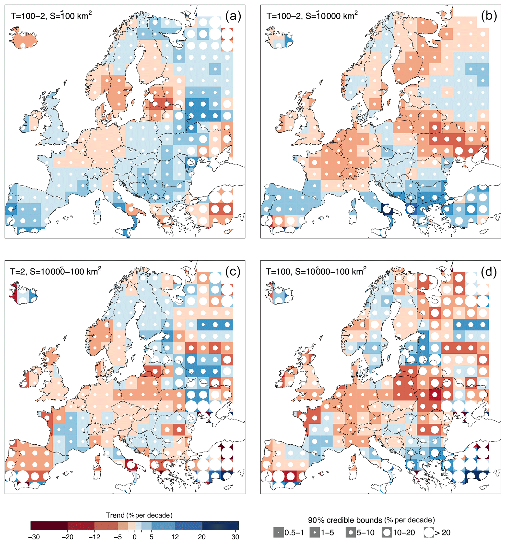
Figure 6 Differences between flood trends of big vs. small floods (i.e. T=100 and 2 years, respectively) and in large vs. small catchments (i.e. S=10 000 and 100 km², respectively). The panels show the differences (in per cent per decade) between the trends of Fig. 5. Positive differences are shown in blue, and negative ones in red. Circle size is proportional to the width of the 90 % credible intervals. The panels in the first row show the difference between the trend in q₁₀₀ and the trend in q₂ for small (a) and big catchment area (b). The panels in the second row show the difference between the trend in large catchments and the trend in small catchments for small (c) and big (d) return periods.

In small catchments (Fig. 6a) positive differences between the trend in q₁₀₀ and in q₂ prevail in the British–Irish Isles, the Iberian Peninsula and southern France, the Balkans, eastern Europe and northern Russia. This indicates that, in the small catchments of these regions, the trend of the extreme flooding events is more positive (or less negative) than the median flood. Negative differences appear in central Europe, the Baltic countries, southern Scandinavia and Turkey. The magnitude of this difference varies in a narrow range (−2 % per decade to +2 % per decade) in most parts of Europe, and it gets larger (up to −12 % per decade to +12 % per decade) in several regions in southern and eastern Europe.

In the case of big catchments (Fig. 6b), negative differences between the trend in q₁₀₀ and in q₂ are more widespread across Europe, compared to those in smaller catchments. In the British–Irish Isles, southern France, northwestern Italy, eastern Europe and northern Russia the difference becomes in fact negative. This suggests that, in the big catchments of these regions, the trend of the extreme flooding events is less positive (or more negative) than the median flood. Positive values of this difference appear mostly in southern Europe and Russia. The magnitude of these differences, in the case of big catchments, varies in a wider range (generally from −5 % per decade to +5 % per decade) with larger differences in few regions in southern and eastern Europe.

The patterns appear more fragmented when analysing the differences between trends in catchments with big and small catchment areas (Fig. 6c and d), and their magnitude is generally larger (mostly from −12 % per decade to +12 % per decade). Negative differences between trends in large catchments and trends in small catchments prevail in western and central Europe (with the exception of France) for both the median and the 100-year flood, and they extend towards eastern countries in the case of the 100-year flood (Fig. 6d). This indicates that trends in large catchments are more negative (or less positive) than those in small catchments. Positive differences appear in central and southern France, the Balkans, the Baltic countries and northern Russia for both T=2 and 100 years (Fig. 6c and d), and in Finland and eastern Europe for T=100 years (Fig. 6d).

3.3 Regional flood regime changes in northwestern, southern and eastern Europe

The regional trends shown in Sect. 3.2 highlight the presence of predominantly positive trends in northwestern Europe and negative trends in southern and eastern Europe. In this section we fit the regional model of Sect. 2.1 by pooling flood data over each of these three regions, and we estimate the regional relative trends for five hypothetical catchment areas (S=10, 100, 1000, 10 000 and 100 000 km²) and for two selected return period values (T=2 and 100 years). The resulting trends are shown together with their 90 % credible intervals in Fig. 7.

Figure 7 Regional relative trend in large (q₁₀₀) vs. small floods (q₂) in (a) northwestern Europe, (b) southern Europe and (c) eastern Europe for five hypothetical catchment areas (S). The figure shows the median (solid dots) and the 90 % credible intervals (error bars) of the posterior distribution of the regional trends. Catchment area is shown with different colours. The figure is obtained for 1985, i.e. the median year of the period analysed.

In northwestern Europe (Fig. 7a) the trends in flood magnitudes are predominantly positive, with the exception of very large catchments for the 100-year flood. The magnitude of the positive trend tends to decrease with increasing catchment area for the 2-year flood, whereas for the 100-year flood the positive trend decreases: it goes to zero for catchment sizes of about 10 000 km² and then becomes negative and increases in absolute value for increasing catchment area. Generally, trends are bigger for the 2-year flood compared to the 100-year flood, with the exception of very small catchments (S=10 km²). Overall there is large variability of the trend in q₁₀₀, which ranges from about −2.5 % per decade to 5 % per decade with catchment area, while the trend in q₂ is around 2–3 % per decade for all areas considered.

In southern Europe the trends are negative in all the considered cases and larger in absolute value for the 2-year flood. This means that the more frequent flood events tend to decrease more than the rare, more extreme events. However, there is small variability of the trends (especially in q₁₀₀) with catchment size. In the smaller catchments the regional relative trends in q₂ and q₁₀₀ are both about −5 % per decade. As catchment area increases, the trend in q₂ decreases from −5.2 % per decade to −7.1 % per decade, while the trend in q₁₀₀ increases from −4.4 % per decade to −3.1 % per decade.

In eastern Europe the regional relative trends are all negative. The estimates lay close to the 1:1 line, which means that the trends are similar for big and small events and that there is little variability with the return period. Catchment area seems to play a more important role in determining flood trends, as the magnitude of the negative trend appears to be very sensitive to the catchment size and ranges from about −13.8 % per decade for the big catchments to −1.9 % per decade for smaller ones.

In all regions analysed, it is also evident that the uncertainties in the trend estimates vary with catchment area: the credible bounds are narrower for mid-sized catchments that are represented by more hydrometric stations in the database.

4 Discussion and conclusions

In this study we assess and compare the changes that have occurred over 5 decades (i.e. 1960–2010) in small vs. big flood events, for catchments of different hypothetical sizes across Europe. We propose a regional flood change model that is more robust than local (at-site) trend analysis, in particular regarding trends associated with large quantiles of the flood frequency curve (e.g. the 100-year flood). Flood peaks are assumed to follow a regional Gumbel distribution, accounting for time dependency of two parameters alternative to the location and scale parameters: the 2-year flood q₂ and the 100-year flood growth factor $x_{\mathrm{100}}^{\prime }$. The two parameters are modelled as varying in time according to log–linear relationships. Other relationships with time could be investigated as well as the use of physical covariates. In flood frequency analysis, the generalized extreme-value distribution (GEV) is commonly used to estimate flood quantiles. The suitability of the GEV distribution in the European context is discussed in detail in Salinas et al. (2014a, b). The estimate of the shape parameter of the GEV distribution is extremely sensitive to record length (Papalexiou and Koutsoyiannis, 2013), with strong bias and uncertainty for short records (Martins and Stedinger, 2000), and, when corrected for the effect of record length, it varies in a narrow range (Papalexiou and Koutsoyiannis, 2013). For these reasons, in regional frequency analyses the GEV shape parameter is commonly assumed to be identical for all sites within a region (see e.g. Renard et al., 2006a; Lima et al., 2016). Here, we fix the shape parameter equal to 0 (i.e. we assume a Gumbel distribution), which leads to more robust relationships without compromising the general validity of the study (i.e. the analysis can be repeated with a more complex GEV distribution if longer flood records are available). A Bayesian Markov chain Monte Carlo (MCMC) approach is used for parameter estimation, allowing information about their associated uncertainties to be obtained directly.

Spatial cross-correlation between flood time series at different sites is not accounted for in this model and may affect the estimation of sampling uncertainty (see e.g. Stedinger, 1983; Castellarin et al., 2008; Sun et al., 2014). Because of this, the sampling uncertainties estimated in this paper should be considered as a lower boundary. We expect that the effect of spatial correlation on the identified spatial patterns is negligible, since the cross-correlation length is about 50 km (calculated from flood time series and distances between catchment outlets, using a non-linear regression model proposed by Tasker and Stedinger, 1989), which is much shorter than the size of the spatial patterns. A possible way of taking into account spatial cross-correlation between sites is a magnitude adjustment to the likelihood, which reflects the overall effect of spatial dependence and results in increased width of uncertainty intervals of the estimated quantiles (see Ribatet et al., 2012). The application of this approach to the specific example region in central Europe shows that the 90 % credible bounds of the regional trends in q₂ and q₁₀₀ are, on average, 20 % wider compared to the case where the likelihood is not adjusted. However, further research is needed to properly characterize the effect of spatial dependence between flood peaks in regional trend analyses.

We analyse 2370 flood records, selected from a newly available pan-European flood database (Hall et al., 2015). We estimate regional trends (and the related uncertainties) in the magnitude of floods of selected return periods (T=2 and 100 years) and for selected catchment areas (S=10 to 100 000 km²), by fitting the proposed regional flood change model to flood data pooled within defined regions. The trend patterns are investigated at the continental scale, by fitting the model to 600 km × 600 km overlapping windows, with a spatial moving-window approach. Flood trends are then analysed in three macro-regions (i.e. northwestern, southern and eastern Europe), based on previously published change patterns of the mean annual flood magnitude and seasonality. When fitting the model to these regions, we allow for local spatial variations in the median but assume homogeneity with regards to the growth curve of flood peaks to changes in time and the dependency of the trends on catchment area and on the return period. The assumption is that these regions are characterized by comparatively homogeneous climatic conditions (and hence flood generation processes) and processes driving flood changes. We have not assessed the statistical homogeneity of the regions in terms of the flood change model used here. One reason is that formal procedures to assess the regional homogeneity, such as those used in regional flood frequency analysis (e.g. Hosking and Wallis, 1993; Viglione et al., 2007), are not available at the moment. Also, while deviation from regional homogeneity would probably invalidate estimates of local flood change statistics from the regional information (e.g. in the prediction in ungauged basins; see Blöschl et al., 2013b), we expect its effect on the average regional behaviour to be less relevant. This is because we have not observed significant differences in the spatial change pattern when changing the size of the moving windows (not shown here). As a limiting case, the results obtained using the three macro-regions (Sect. 3.3) are consistent with those obtained by the moving-window analysis across Europe (Sect. 3.2).

The results of this study show that the trends in flood magnitude are generally positive in northwestern Europe, where floods occur predominantly in winter (Mediero et al., 2015; Blöschl et al., 2017; Hall and Blöschl, 2018). The increasing winter runoff in the UK is typically explained in the literature by increasing winter precipitation and soil moisture (Wilby et al., 2008). Recent studies show that extreme winter precipitation and flooding events in northwestern Europe are positively correlated with the North Atlantic Oscillation and the east Atlantic pattern (Hannaford and Marsh, 2008; Steirou et al., 2019; Zanardo et al., 2019; Brady et al., 2019). Furthermore the largest winter floods in Britain occur simultaneously with atmospheric rivers (Lavers et al., 2011), which are expected to become more frequent in a warmer climate (Lavers and Villarini, 2013). When comparing trends in flood events associated with different return periods, we observe two opposite behaviours depending on catchment area. In small catchments (up to 100 km²) the 100-year flood increases more than the median flood, while the opposite is observed in medium and large catchments, where even some negative trends appear, especially in northwestern France. Furthermore, in medium and large catchments the magnitude of the trends is in general smaller compared to the small catchments. This could be explained by different types of weather events and their changes affecting the flood trends in catchments of different sizes in different ways; for example, long-duration synoptic weather events are probably more influential in producing floods in medium and large catchments, in contrast to small catchments in western Europe, where the largest peaks are often caused by summer convective events with high local intensities (Wilby et al., 2008), which are expected to increase in a warmer climate (IPCC, 2013).

In southern Europe flood trends are negative, possibly due to decreasing precipitation and soil moisture, caused by increasing evapotranspiration and temperature (Mediero et al., 2014; Blöschl et al., 2019). The big flood events (i.e. T=100 years) decrease less in time compared to more frequent events (i.e. T=2 years), leading to higher flood variability and steeper flood frequency curves. The reason for this may be (decreasing) soil moisture driving flood changes in southern Europe, causing drier catchments and consequently negative trends in flood magnitudes that are particularly strong for small floods (q₂), where the influence of soil moisture is stronger (as shown e.g. by Grillakis et al., 2016). The magnitude of big flood events is also decreasing (probably as an effect of decreasing precipitation), but in this case soil moisture is less influential, resulting in less strong negative trends compared to q₂. The flood trends do not vary significantly with catchment area. In smaller catchments we observe similar negative trends in q₂ and q₁₀₀ (about 5 % per decade). With increasing catchment area the trends in q₂ become more negative, while the opposite is observed for q₁₀₀. Notice, however, that the small catchments analysed in southern Europe have sizes of the order of 10 km² and are, therefore, larger than catchments where flash floods are the dominant flood type and infiltration excess runoff is the main generation mechanism (Amponsah et al., 2018). For these very small catchments (< 10 km²), floods may become larger due to more frequent thunderstorms (Ban et al., 2015) and land management changes, e.g. deforestation and urbanization (Rogger et al., 2017).

In eastern Europe trends in flood peak magnitude are strongly negative for both small and big floods in small to large catchments. These negative flood trends have been linked in past studies with increasing spring air temperature, earlier snowmelt and reduced spring snow-cover extents (Estilow et al., 2015), producing increased infiltration and consequently earlier and decreasing spring floods (Madsen et al., 2014; Blöschl et al., 2017, 2019). The resulting trends in eastern Europe do not seem to depend on the return period (i.e. for a given catchment area, the trend in q₂ and the trend in q₁₀₀ are almost identical), whereas catchment area plays a substantial role: the larger the catchment area, the more negative the trend. These results suggest that, in this region, snowmelt affects flood events of different magnitude in the same way and represents a relevant processes for flood (trend) generation especially in large catchments. The explanation for the importance of these processes in large catchments could be found in the characteristics of snowmelt flooding, which originates from large-scale gradual processes, i.e. snowfall and temperature changes, that may be more influential for large-scale events compared to smaller-scale catchments, where other local conditions may prevail.

The uncertainty associated with the regional trend estimates is here assessed through their 90 % credible bounds. The results show that the uncertainties in the trend estimates vary with catchment area: the credible bounds are generally narrower for mid-sized catchments, which are represented by more samples in the database, and the bounds become wider for very small and very large values of catchment area, where fewer samples are available. Spatial patterns in trend uncertainties are also observed. As expected, the uncertainty is lower in the regions where the density of stations is very high (i.e. central Europe and UK), while the estimated trend is very uncertain in the data-scarce regions (i.e. southern and eastern Europe).

This study provides a continental-scale analysis of the changes in flood quantiles that have occurred across Europe over 5 decades; however further research is needed to formally attribute the resulting regional change patterns to potential driving processes. According to flood hazard projections, the past flood regime changes found in this study are likely to further occur in the next decades, led by increasing precipitation over northwestern Europe, decreasing precipitation over southern Europe and increasing temperature in eastern Europe (see e.g. Alfieri et al., 2015; Kundzewicz et al., 2016; Thober et al., 2018). This has relevant implications since flood risk management has to adapt to these new realities.

Appendix A

Figure A1 Number of stations in each 600 km × 600 km region, stratified by catchment size: (a) 10 to 100 km², (b) 100 to 1000 km², (c) 1000 to 10 000 km² and (d) 10 000 to 100 000 km². The value representative for the region is plotted in the respective central 200 km × 200 km cell.