the Creative Commons Attribution 4.0 License.
the Creative Commons Attribution 4.0 License.
 | 11 Mar 2020
Hydrograph separation: an impartial parametrisation for an imperfect method
Antoine Pelletier
Vazken Andréassian
This paper presents a new method for hydrograph separation. It is well-known that all hydrological methods aiming at separating streamflow into baseflow – its slow or delayed component – and quickflow – its non-delayed component – present large imperfections, and we do not claim to provide here a perfect solution. However, the method described here is at least (i) impartial in the determination of its two parameters (a quadratic reservoir capacity and a response time), (ii) coherent in time (as assessed by a split-sample test) and (iii) geologically coherent (an exhaustive validation on 1664 French catchments shows a good match with what we know of France's hydrogeology). With these characteristics, the method can be used to perform a general assessment of hydroclimatic memory of catchments. Last, an R package is provided to ensure reproducibility of the results presented.
- Article
(3716 KB) - Full-text XML
-
Supplement
(189 KB) - BibTeX
- EndNote


Hydrograph separation and the identification of the baseflow contribution to streamflow is definitely not a new subject in hydrology. This age-old topic (Boussinesq, 1904; Horton, 1933; Maillet, 1905) is almost as universally decried as it is universally used. Indeed, two adjectives appear repeatedly in hydrology textbooks: artificial and arbitrary (see e.g. Linsley et al., 1975; Réméniéras, 1965; Roche, 1963; Chow, 1964). Hewlett and Hibbert (1967) – the famous forest hydrology precursors – even added desperate, where Klemeš (1986) compared the hydrograph separation procedures with the astronomical epicycles (i.e. the absurd trajectories that had been invented to maintain the geocentric theory before the time of Copernicus and Galilei).
To assess baseflow, direct measurement is generally impossible, since it is a conceptual quantity, not a physical one. Proxy approaches involving chemical tracer-based procedures are efficient but need chemical data and involve their load of assumptions. Most approaches rely on solving an inverse problem, i.e. reckoning the quantitative causes (here baseflow and quickflow) of an observed physical phenomenon – total runoff. This procedure is very common in hydrology; it is reasonably feasible when the variable can be measured and a calibration procedure can be implemented. But here again, the non-measurable character of baseflow renders the question difficult.
It is perhaps impossible to propose a physically based baseflow separation procedure (just because of the multiplicity of flow paths that makes the procedure fundamentally equifinal), and we will not argue about this point. But we believe that even the imperfect conceptual–mathematical–empirical methods in use could receive a non-arbitrary, impartial, repeatable parametrisation that could be used as a general-purpose study tool over large catchment sets.
This paper focuses on a hydrograph separation method that is based only on quantitative streamflow data and climate descriptors and does not require a priori physical parametrisation, presented in Sect. 2. The originality of this method lies in its parametrisation strategy, which we discuss in detail in Sect. 2.2. The application of this procedure to a set of 1664 catchments, its geological coherence and its stability in time are presented in Sect. 3.
1.1 The principle of hydrograph separation
Hydrograph separation is based on the following assumption: streamflow can be divided into two components, baseflow and quickflow, whose response to hydroclimatic events is different. Baseflow is the slow component of streamflow, while quickflow in the remaining part, i.e. the quick part of streamflow. This separation in two components is obviously artificial: there is generally a wider range of hydrological processes at stake that respond diversely to hydroclimatic events. Having said that, it is still possible and interesting to set up an arbitrary barrier between the not-too-delayed components of streamflow – quickflow – and the delayed-enough components – baseflow.
A commonly found definition of hydrograph separation is splitting streamflow between surface runoff and groundwater contribution. This may be an acceptable interpretation of chemicophysical methods that are based on the difference – of composition or temperature, for instance – between different sources of water. However, process interpretation of hydrograph separation is a generally hazardous practice (Beven, 1991). If surface runoff is definitely one of the quicker hydrological processes, a quick response to a rainfall event is not necessarily composed of recent water; it can even be made of mostly old water (Kirchner, 2003). At the scale of a single event, defining baseflow as groundwater contribution results from confusion between celerity and velocity of the hydrograph response (McDonnell and Beven, 2014): baseflow is composed of perturbations propagated with a low celerity and much dispersion, which can be composed of old and recent water coming from various stores, such as subsurface flow, aquifers or bank storage. Therefore, baseflow is the component of the hydrograph bearing the catchment's memory.
Existing procedures for hydrograph separation and baseflow assessment can be sorted into three categories (Gonzales et al., 2009), according to their level of physicalness: (i) physical and chemical methods are based on chemicophysical differences between quick water and slow water, assuming that they come from different sources; (ii) numerical and empirical methods which do not attempt any kind of hydrological representation or modelling and use signal processing tools to alter streamflow hydrographs; and (iii) conceptual methods which conceive of baseflow as the outflow of a reservoir that represents the catchment's memory. The following sections provide an overview of these three categories, before concluding about their shortages and drawbacks that led to the development of a new method.
1.2 Chemicophysical methods
Chemicophysical methods are based on the fact that total flow is a mix of various sources of water, with different characteristics (Pinder and Jones, 1969). By accounting for the latter, it is possible to revert mixing equations to get the relative contribution of each flow source, using a simple mass-balance approach. Chemicophysical methods are powerful; they provide a lot of information where water quality data are available and where the hydrochemical configuration allows for rather strong hypotheses: consistency in space and time of water characteristics and the assumption that the hydrological system is conservative – to avoid any unknown water inflow.
The most common methods of this family are tracer-based baseflow separations. A passive tracer whose concentration is different in groundwater, subsurface, bank and surface runoff water – for instance, isotopes (Cartwright and Morgenstern, 2018) such as deuterium, tritium or 18O, ions (carbonates, calcium, magnesium or sulfates) from dissolved minerals, or silica – is used as a proxy for mass balance assessment; at each time step of available data, it allows for a dynamic real-time baseflow decomposition. Other methods rely on conductivity, pH or temperature, which can be easier to measure in situ.
There are three main drawbacks in chemicophysical methods. First, the inherent uncertainties: there are measurement errors; concentrations can have spatial and temporal heterogeneity, even within the same rainstorm; and the passiveness of tracers may not be a valid hypothesis even in short events. Kirchner (2019) proposed a statistical tracer-based separation to replace this mass balance hypothesis, using a regression between baseflow and tracer concentrations in streamflow and rainfall. Second, the implementation of these methods on catchments is limited by the large amount of required data. Continuous groundwater and surface water quality data are seldom available except for specially instrumented catchments (Gonzales et al., 2009). Finally, they imply a process-based definition of baseflow and quickflow, which is difficult to build without knowing the particular context of each catchment; that is why tracer-based methods generally give different results with respect to conceptual and numerical methods (Cartwright et al., 2014; Costelloe et al., 2015). Even though tracer-based methods can provide useful and valuable information on dominant processes occurring inside a catchment, their application for routine analysis is not conceivable on a large number of gauging stations.
1.3 Empirical and numerical methods
Several classic baseflow separation methods are not based on hydrological considerations, but they rely on processing the hydrograph as a signal. Most of these methods are based on the hypothesis that the transfer time of surface runoff is much shorter than that of groundwater, and that this time is relatively constant between rainfall events. The first methods of this type were graphical. After identifying peaks along the hydrograph and estimating the surface runoff time constant – let us say N d – peaks are cut by drawing a straight line between the beginning of each peak and the point N d after (Linsley et al., 1975; Gonzales et al., 2009). This simple approach has been enhanced to take into account consecutive precipitation events or aquifer recharge during rainfall, but it remains quite subjective, as the graphical processing is supposed to be done by hand and is difficult to automatise. Streamflow under the constructed dividing line is assumed to be baseflow, while the remaining peaks are surface flow.
Within the same set of hypotheses, low-pass numerical filtering of the hydrograph has been used as a baseflow separation method. As in electronic signal filtering, the highest frequencies of the signal are dropped; and the low ones are kept. Fourier-transform-based filters implement this framework, but they are intended for data with stationary periodic processes, whereas hydrological signals operate on a very large range of timescales. Even quick components of streamflow have low-frequency Fourier terms (Duvert et al., 2015; Labat, 2005; Su et al., 2016). Classical electronic low-pass filters are therefore not adapted to hydrograph separation. In line with graphical methods, a local minimum filter on a sliding window – whose length is basically the timescale of baseflow – has been developed, as well as recursive digital filters with low-pass properties. Transformations can be applied on the streamflow time series before numerical filtering, in order to improve the filter's efficiency (Romanowicz, 2010). Finally, artificial neural networks have been employed as data-driven models for hydrograph separation (Taormina et al., 2015; Jain et al., 2004).
Numerical methods all need one or several parameters, with or without hydrological meaning, which have to be valued before processing: time interval width, coefficients of a linear filter, formula of the transformation function, etc. Even though authors generally give advice about the possible values of these parameters, determining them involves adding new hypotheses for each catchment examined (Eckhardt, 2005, 2008; Mei and Anagnostou, 2015). In particular, quantitative results of the filtering change with the value of the parameters. Although the shape of the hydrograph separation can be visually consistent with the conceptualisation of a hydrograph separation, it is basically impossible to draw any conclusion from it.
1.4 Conceptual methods
In addition to chemicophysical and numerical methods, another way of separating hydrographs has been developed, starting from the idea that the slow parts of catchments can be represented as conceptual reservoirs, whose outflow is baseflow. Such an approach comes from the analysis of long recession curves and the inference of depletion laws, which rule streamflow during long, dry periods of low flows. By knowing the outflow law of the conceptual reservoir, assuming that its input is zero, it is possible to get the full recession curve by the next significant rainfall event (Coutagne, 1948; Wittenberg, 1994). In practice, various types of reservoirs are implemented in this type of model: linear, quadratic and exponential are the most common (Bentura and Michel, 1997; Michel et al., 2003).
It is possible to calibrate such a model by fitting it on long recession curves, but the latter have to be defined, for instance, through a threshold on streamflow – considering that only low flows correspond to recessions – or on its derivative, possibly with a smoothing filter – such as a moving average or sliding window minimum – in order to eliminate noise in the signal. Such a sampling of the hydrograph can be difficult to make without arbitrariness, either in the value of thresholds or in smoothing filters. Existing studies generally focus on a particular recession, for instance, along a drought in which streamflow is known to have been measured well (Wittenberg and Sivapalan, 1999; Wittenberg, 1994; Coutagne, 1948). It may be impossible to find such a drought to respect the zero-input hypothesis: in western Europe, for instance, rainstorms at the end of summer often disrupt the low-flow signal.
To filter the whole hydrograph with this conceptual idea of baseflow, a backward filter was developed by Wittenberg (1999). The hydrograph is traced back with reservoir recession curves; the level of the reservoir increases as depletion is followed backward and reinitialised when the peak is reached. Some arbitrariness remains in the value of the reservoir parameter. Moreover, whereas this method yields visually consistent hydrograph separations with wide time steps, baseflow may not be smooth enough under flood peaks: a further smoothing is thus needed and constitutes, here again, a source of partiality.
1.5 Elements of comparison and coupling between methods
Although it is impossible to perform an absolute evaluation of a hydrograph separation method, since baseflow cannot be measured and compared with a simulated value, several comparative studies have challenged results from various methods. Chemicophysical and non-calibrated graphical and empirical algorithms – i.e. without parameters or whose parameters are determined a priori and do not vary between catchments – have given very different results (Kronholm and Capel, 2015; Miller et al., 2015; Lott and Stewart, 2016; Cartwright et al., 2014). It is therefore difficult to use non-calibrated empirical or graphical hydrograph separation methods as general-purpose analysis tools.
To overcome this issue, several studies use parametric graphical and empirical methods and calibrate them with chemicophysical data (Saraiva Okello et al., 2018; Miller et al., 2015; Chapman, 1999). It allows one to extend the hydrograph separation on time periods where chemicophysical data are not available, or to perform temporal downscaling – when, for instance, daily streamflow data or monthly tracer concentrations are available. Such calibrated parametric algorithms have given satisfying results. Chapman (1999) highlighted that adding parameters to a hydrograph separation algorithm does not necessarily improve performance, since the algorithm becomes harder to calibrate.
When performing a large-scale baseflow analysis over a territory, it is possible to extend calibrated parameters at gauged catchments to ungauged ones through regionalisation models. Singh et al. (2019) performed such a study over the entire territory of New Zealand. We decided to limit ourselves to gauged catchments for this work.
1.6 Synthesis and guidance for this work
Most of the methods above rely on one or several parameters whose value has a strong influence on hydrograph separation; as it is impossible to calibrate this – or these – parameter(s) on the basis of a measurement, some physical hypotheses must be made on the desirable properties of baseflow, in relation to the memory of the catchment. Non-calibrated algorithms are not usable as general-purpose analysis tools and existing calibration procedures rely on the availability of chemicophysical data. In this work, we propose a calibration procedure of a conceptual hydrograph separation method that relies only on hydroclimatic data: streamflow, rainfall and temperature.
Frugality and objectivity do not only result in a small number of parameters. The choice of modelling options can also be a source of arbitrariness and useless complication. A modelling alternative can, moreover, be solved only through a personal choice of the modeller; one way to create a trustworthy framework is to build it upon well-known and well-validated elements that have proven themselves relevant in lumped conceptual hydrology. Beyond the complexity of elements, there is the complexity of the modelling chain itself. The simpler the model is, the more readable and thus the less questionable it is; in this work, it was considered that a baseflow separation process should be much simpler than, for instance, a lumped conceptual model designed for flow simulation.
2.1 Digital filtering based on conceptual storage
In this paper, we postulate that the memory and smoothing effect of a catchment – which underpins the concept of baseflow – can be represented by a conceptual reservoir, whose outflow will depict the delayed contribution to streamflow, which we will assimilate into baseflow. To be applied in practice, this postulate must be complemented by an answer to the two following questions: what should the input to the reservoir be? What should the relationship between the level of the reservoir and its outflow be?
2.1.1 Discharge as a proxy of recharge
The first question asks what should refill the conceptual reservoir (i.e. what recharges the catchment with water that will be baseflow afterwards). The part of rainfall that does not contribute to surface runoff or to evaporation is generally named recharge, as it is thought to feed groundwater storage. It is common to estimate the recharge function through a surface water budget model, which computes it from climatic information (rainfall, evapotranspiration, temperature, etc.), as it is done more or less complexly in common rainfall–runoff models or in soil–vegetation–atmosphere schemes. A physical separation between hydrological processes would need such production modules, but it is not the scope of our conceptual method; we do not try to estimate the groundwater recharge but instead the fraction of water that will contribute to the delayed component of streamflow.
The general contribution of this conceptual memory recharge is supposed to be an increasing function of streamflow: a flood event will lead to a more humid behaviour of the catchment months after, while a drought will decrease baseflow for several years. That is why we make the hypothesis that the best candidate for a proxy of this conceptual recharge is a linear fraction of total flow itself. It is available without a further model or hypothesis. But using a linear fraction of total flow raises an issue: if x % of total flow is poured into the reservoir and baseflow, which represents on average y % of total flow, and is taken out of the reservoir, then the water budget of the filtering process will only be balanced if x=y. The parametrisation strategy takes this problem into account; it is presented in Sect. 2.2.
2.1.2 Reservoir filtering
The filtering part of the method is a conceptual reservoir, whose inflow is a fraction of the total observed flow at the gauging station, and the outflow is regarded as baseflow. The content of this reservoir is managed by an outflow function and a continuous differential equation: since data are obviously available as discrete time series with a time step Δt, it is necessary to discretise this equation to set the numerical filtering algorithm.
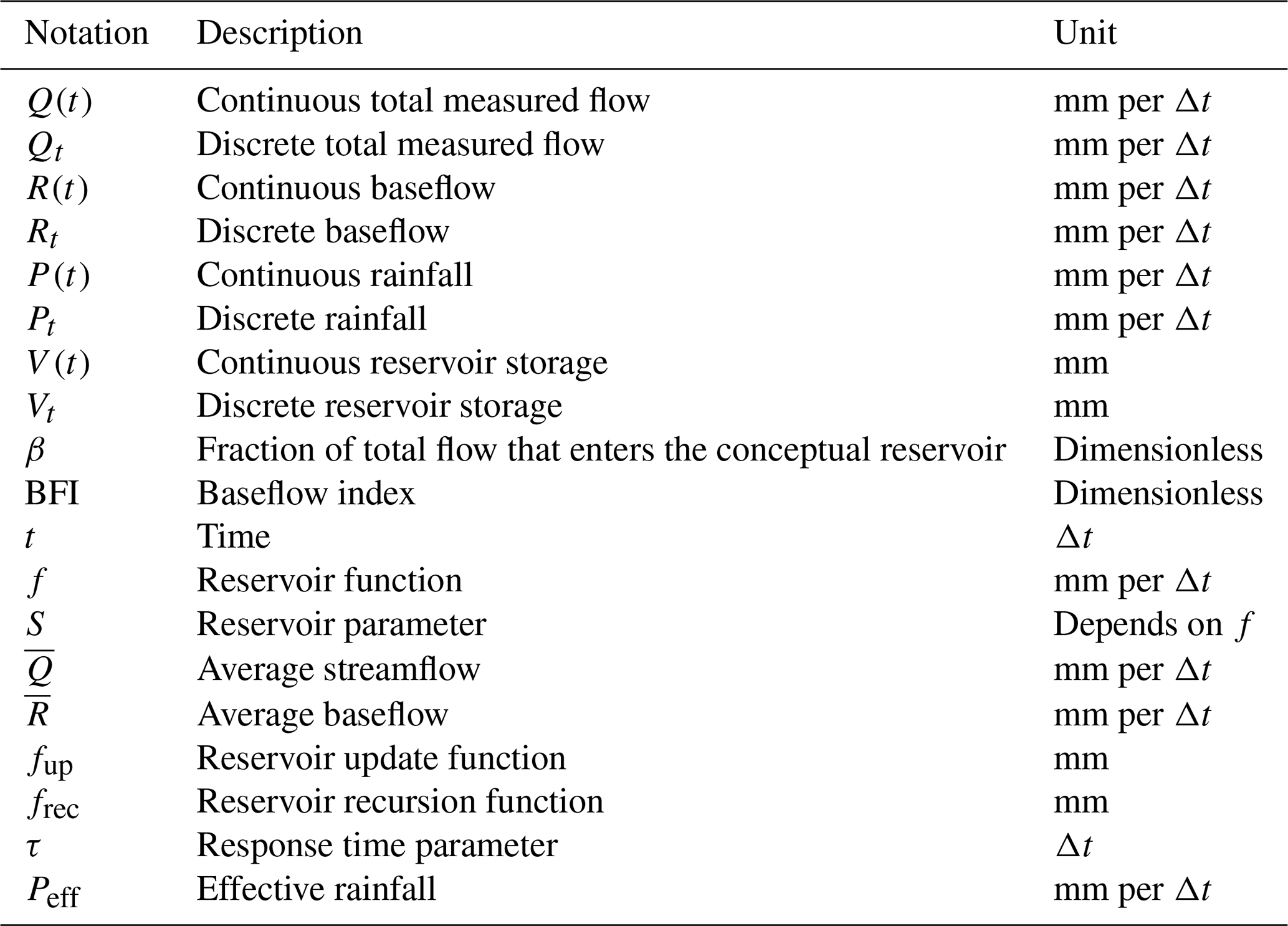
The notations listed in Table 1 will be used henceforth. All variables are expressed as intensive values – i.e. as depths in millimetres for precipitation, flows and reservoir storage – in order to avoid conversions with the basin area.
According to the definition of a reservoir, V(t) is governed by the following system of equations:
where f is the outflow function of the reservoir, with a parameter S, whose dimension depends on the formula of f. Many functions can be imagined, but the most common ones are the following (Brodie and Hosteletler, 2005):
-
linear reservoir: ;
-
quadratic reservoir: ;
-
exponential reservoir: .
Linear reservoir has been widely used because of computation ease and direct analogy with linear filtering systems: the reservoir can be, for instance, assimilated into a low-pass electronic filter; the comparison with a capacitor and a resistor is quite straightforward. On the contrary, computations with the two other functions involve solving a non-linear differential equation, which removes the analogy with classical linear filters. Notwithstanding these practical considerations, groundwater discharge is fundamentally a non-linear phenomenon. Several authors (Coutagne, 1948; Wittenberg, 1994, 1999; Bentura and Michel, 1997) have argued that from a general-purpose point of view, a quadratic reservoir is the most adapted function. It has been derived from statistical studies of various catchments, together with theoretical studies of springs and unconfined aquifers. Therefore, a quadratic reservoir is chosen for this work.
In order to discretise the filter, we define discrete versions of continuous variables cited above. If X(t) is continuous, for a discrete time step t, we define Xt=X(t). To integrate Eq. (1), a direct integration scheme is performed: at each time step t, βQt is added to the reservoir at the beginning of the time interval , and the differential equation is solved on this time interval.
Although it is done in most conceptual hydrological models, integrating differential equations using this method in a discrete hydrological model could be criticised (Fenicia et al., 2011; Ficchì, 2017) because the explicit Euler integration scheme is not stable in solving many ordinary differential equations. For instance, it can lead to diverging numerical solutions, while analytical ones are supposed to be bounded. We find it acceptable to use this explicit integration scheme for the sake of simplicity, given that divergence of the result is controlled by the reservoir update detailed in Sect. 2.1.3.
Thus, just before , and just after . With a quadratic reservoir function, Eq. (1) can now be written on the time interval .
After integration, the discrete recursive equation is
where Rt is the total outflow during the time interval []. From another integration of Eq. (1), a balance equation is obtained: . Therefore, using Eq. (4), the following formula for Rt is obtained.
Note that these equations have a conceptually coherent behaviour: Vt and Rt are always positive; without inflow, Eq. (4) becomes a depletion equation, which converges to zero; the reservoir empties itself all the faster as its level is high; and S acts as a capacity; i.e. at the end of a time step, the level of the reservoir is always lower than S.
2.1.3 Reservoir update
The filtering process detailed above raises an issue: baseflow is by definition a fraction of total flow; yet, Eq. (5) does not guarantee that Rt is lower than Qt. Conceptual rainfall–runoff models classically rely on evaporation or on a leakage function to empty their reservoirs. Here, in order to avoid adding unnecessary complexity, it was decided to perform a simple update of the reservoir level when the outflow is greater than the measured flow. Although it may seem quite brutal, it must be seen as a readjustment of the model after a flood peak, in order to fit the observed flood recession. Since part of streamflow is only used as a proxy of recharge, and is therefore not the recharge itself, it can only be an imperfect input data for the model, and thus a correction process within the latter is not a surprise.
If Rt is computed as greater than Qt, the level of the reservoir Vt needs to be updated so that Rt=Qt, which leads, through a simple balance of the reservoir, to . Equation (6) then gives the update function, by solving a quadratic polynomial equation.
Here again, Vt is always non-negative and strictly lower than S. The formula above artificially creates a numerical exception when Qt=0, which must be taken into account in the implementation of the algorithm, with Vt=0.
This update process takes water out of the reservoir when computed baseflow is too high; but do we not need to correct baseflow when it is too low? Indeed, quickflow is supposed to be zero during long, rainless, dry periods. For the sake of simplicity, a straightforward hypothesis is added: baseflow must be equal to total flow at least once in a hydrological year, when measured streamflow reaches its yearly minimum. The value of the latter can be affected by measurement errors, but it is hard to take it into account in a general-purpose analysis tool: the structure of the error is determined by the idiosyncrasies of each catchment. Moreover, the two ways of updating the reservoir helps the model to forget about previous errors; therefore, we prefer not to add another hypothesis about the low-flow measurement uncertainty.
A test study is performed on a set of catchments in continental France: thus, the low-flow hydrological year is taken from 1 April to 1 March, as streamflow minima do not generally occur during spring. The Qt time series is then divided into hydrological years, and for each of them, a minimum value and its index are computed. If the series is n – hydrological – years long, it creates a set of n points where the reservoir level is updated through Eq. (6) so that Rt=Qt.
This second update process adds water to the reservoir; it is thus possible to balance the updates of the reservoir and, thereby, to balance the total water budget of the filtering process. If and are the means of time variables Qt and Rt, the water budget is given by Eq. (7).
where BFI is the baseflow index, namely, the long-term ratio of the computed baseflow to total measured streamflow, i.e. BFI = . Equation (7) gives a simple parametrisation constraint to ensure a balanced water budget: β = BFI.
The yearly minimum update may look too strong and arbitrary, but tests have shown that it is necessary to avoid issues in the parametrisation strategy: removing it adds a third degree of freedom in calibrating the model – the value of β, which is not constrained to be equal to BFI – which leads to optimisation problems while calibrating the algorithm.
2.1.4 Initialisation
Our algorithm does not need a long warm-up period, as required by rainfall–runoff models. Since the algorithm presented above contains only one state and involves a regular update with observed data, this update erases the memory of the past states of the model. Therefore, a simple initialisation approach is possible. Several methods were tested, and the best compromise between simplicity and robustness was adopted. The reservoir level is initialised through Eq. (6), using mean flow over a small time period – five time steps – at the beginning of the flow time series. To avoid any overestimation of baseflow at the beginning of the hydrograph, computations were started far from any flood events: 1 August is a convenient date for continental mainland France, since no French river has major high-flow episodes in mid-summer.
2.1.5 Synthesis of the algorithm
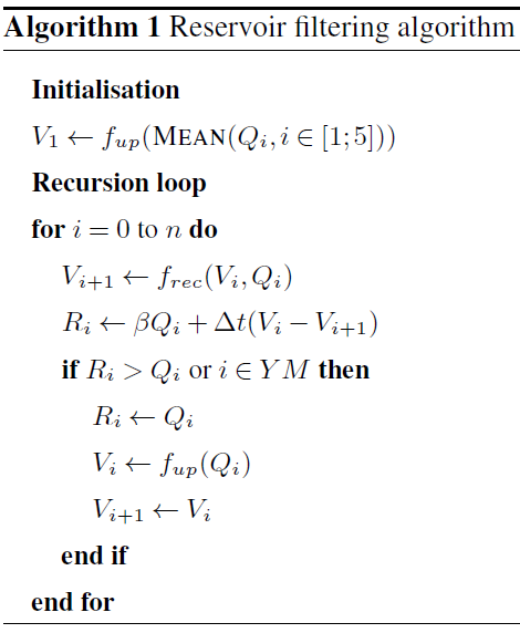
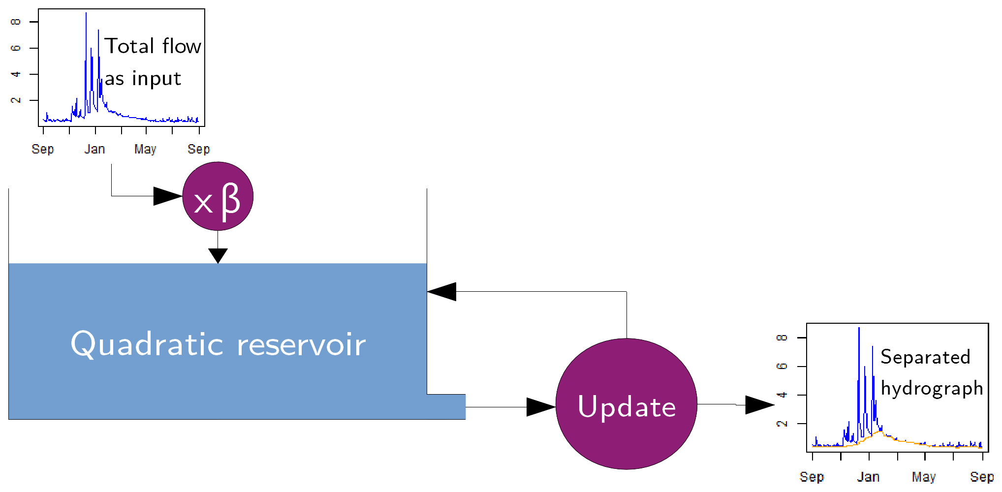
Finally, the filtering algorithm can be summarised with the pseudo-code detailed in Algorithm 1, where fup(Qt) is the update function of Eq. (6), frec(Vt,Qt) is the recursion function of Eq. (4), n is the number of time steps and YM is the set of indexes of yearly minima. Figure 1 synthesises the principle of the algorithm.
2.2 Parametrisation strategy
As stated above, the difficulty of parametrisation comes from the fact that baseflow cannot be measured. In the absence of measurement, we need to make a hypothesis concerning a desirable property of the computed baseflow, in order to be able to look for the parameter set that will best respect this property. Since baseflow accounts for the slow component of total flow, coming out of the storage parts of a river basin, we make the following hypothesis: baseflow should be correlated with past climatic events that have filled or emptied this storage; and since it is supposed to be slow, it should be correlated with events that happened quite a long time ago. The calibration criterion has to be a simple quantification of this idea, which corresponds to the concept of recharge stated earlier: a proxy of past recharge must be found.
The filtering algorithm detailed above depends on two parameters: capacity S of the reservoir and scaling factor β. Yet, with the water balance condition given by Eq. (7), it is possible to remove 1 degree of freedom: for a given value of S, function is injective; therefore, there is a unique value of β that fulfils BFI, and the β(S) function can be identified.
After eliminating 1 degree of freedom, the correlation hypothesis stated above can be converted into a criterion: it computes Pearson's correlation between the computed baseflow time series – which depends on the reservoir's parameter S – and cumulated effective rainfall on the τ days before each time step. The first τ−1 values of the baseflow time series thus do not influence the criterion, since the first τ−1 values of the cumulated effective rainfall time series are missing values, and, therefore, they are eliminated when computing Pearson's correlation; this limits the effect of model initialisation. If Peff,t is the daily effective rainfall value on day t, the criterion is written as:
This correlation must be maximised to yield two pieces of information: the optimal value Sopt of the capacity of the reservoir, which gives a hydrograph separation, and a conceptual response time τopt of the catchment to hydroclimatic events, which can be compared with other pieces of knowledge about its behaviour, in order to assess the separation method's relevance.
As far as the optimisation process is concerned, it is necessary to define search intervals for S and τ. For S, values lower than 1 mm were not observed during tests and led to computation issues; thus the lower bound can be set at 1 mm. On the other side of the search interval, values around 106 mm – i.e. 1 km – were found during tests, without leading to incongruities in baseflow separation. Therefore, it is suggested to set the upper bound to 2×106 mm. For τ, typical values are between 3 months and 1 year: the search range is then set to [5; 1825] d. Note that during tests, τ optimal values were easier to find than S values.
Effective rainfall was computed with the Turc–Mezentsev formula (Turc, 1953; Mezentsev, 1955), with a quadratic harmonic mean between potential evaporation (PET) and rainfall, i.e.
where Ptot is daily total rainfall and PET is daily potential evapotranspiration, computed with Oudin's formula (Oudin, 2004; Oudin et al., 2005). Effective rainfall is thus computed at a daily time step and aggregated to get the criterion defined by Eq. (8). By way of comparison, alternative ways of computation were tried: the Penman–Monteith formula for PET (Monteith, 1965) and simple screening of rain by PET for effective rainfall, i.e. . No major difference was found in the results.
Therefore, we found an effective parametrisation strategy for choosing the three parameters β, S and τ. β is first linked to S through the budget condition given by Eq. (7), which removes 1 degree of freedom; then, the two remaining parameters S and τ are chosen by optimising the correlation criterion given by Eq. (8).
2.3 Catchment dataset
Several hydrographic regions of mainland France are influenced by large aquifers, which bear the memory of past climatic events and have a significant contribution to river flow. In the Paris basin, the chalk aquifer – composed of late Cretaceous formations – has a significant connection with many rivers in the Seine and the Somme basins, which notably led to major groundwater-induced floods after the extremely wet years of 1999 and 2000 (Pinault et al., 2005; Habets et al., 2010). The Loire basin is linked to the Beauce aquifer, mostly made of tertiary layers, whose situation under a large agricultural plain induces water management issues that affect Loire low flows. The international Rhineland aquifer, part of which extends to Alsace, also plays a major role in the hydrology of the Rhine.
Tests were performed on a set of 1664 catchments that were selected on the basis of diversity of area, climate, hydrological regime and completeness of the time series in the period 1967–2018. Streamflow data are from the national database Banque Hydro (SCHAPI, 2015; Leleu et al., 2014), where measurements regarded as unreliable were converted into missing values. Climatic data are from the SAFRAN (Système d'Analyse Fournissant des Renseignements Adaptés à la Nivologie; Analysis System for Providing Atmospheric Information Relevant to Snow) reanalysis (Vidal et al., 2010), developed by Météo France and aggregated for each catchment, to get a lumped climatic series of rainfall and PET. The combination of the SAFRAN and Banque Hydro data is stored in the HydroSafran database, maintained and hosted by INRAE (French National Research Institute for Agriculture, Food and the Environment; Delaigue et al., 2020).
Gaps in the streamflow time series were filled using simulated flows from the daily lumped rainfall–runoff model GR4J (modèle du Génie Rural à 4 paramètres Journalier; daily four-parameter model from the rural engineering service) (Perrin, 2002; Perrin et al., 2003), calibrated on the whole period 1968–2018, we make the hypothesis that hydrological characteristics of catchments are stationary all along this period. The chosen catchments have more than 20 complete years – a hydrological year is regarded as complete when there is no gap longer than a week and the total proportion of missing values is lower than 5 %. The filling simulation model GR4J has a good performance, with a Nash–Sutcliffe criterion higher than 0.7. All computations were performed with R and the airGR package for specific hydrological processing (Coron et al., 2017, 2020).
Tables 2 and 3 show some characteristics of the catchment dataset: it is representative of the climatic and landscape diversity in mainland France. We chose basins with a large range in size, from very small (less than 2 km2) to very large (117 000 km2). A quick geological analysis of the 1664 catchments was also performed based on the national hydrogeological map by Margat (1980). It highlighted that 1310 catchments are not very likely to be influenced by aquifers, since they are on impermeable formations, such as igneous or metamorphic rocks or clay; 122 catchments have more than 90 % of their surface on sedimentary formations that are likely to carry large aquifers; and 232 catchments have a mixed configuration. Figure 2 shows the geographic repartition of the catchment set.
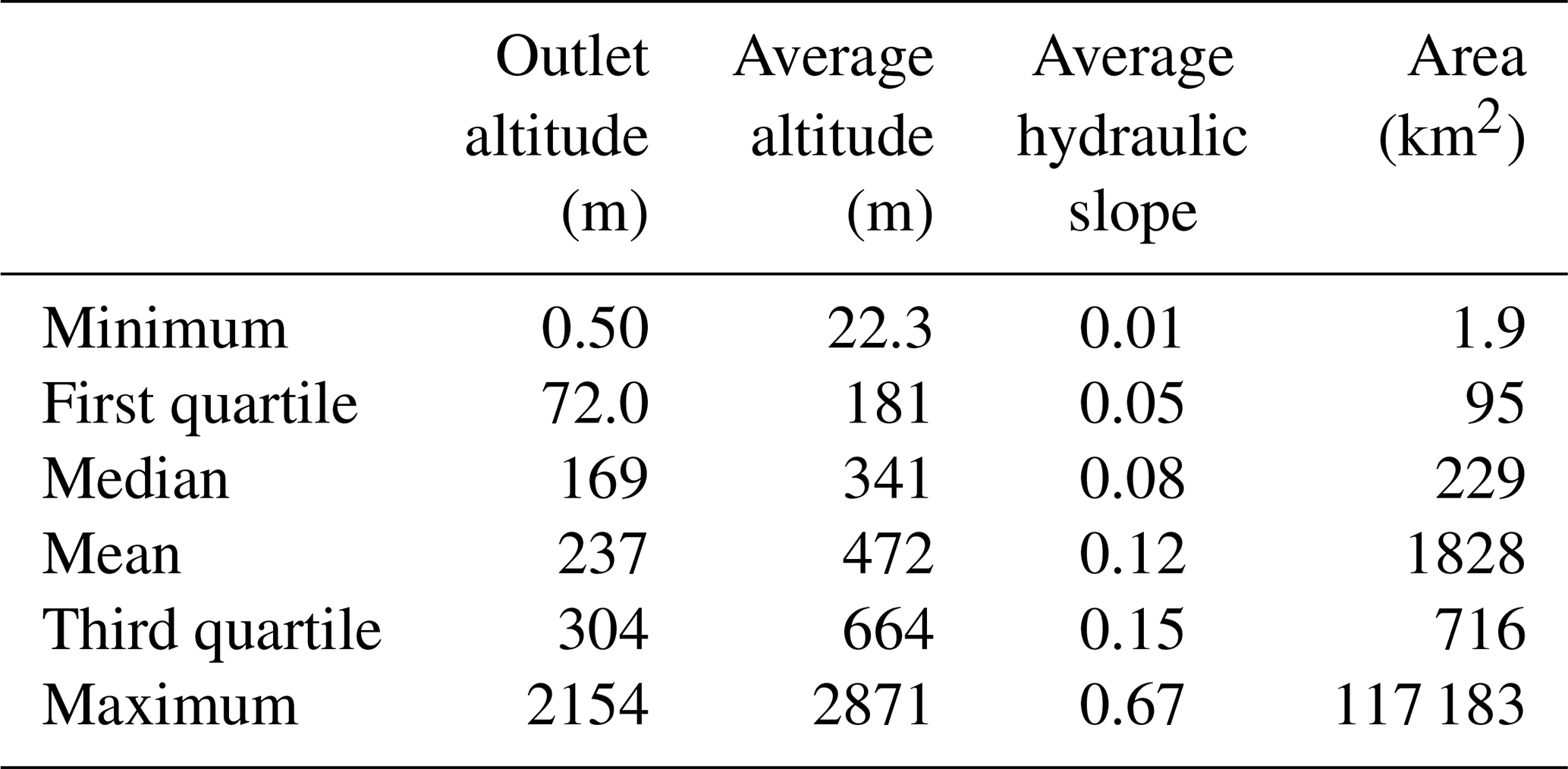
Table 3Hydrological characteristics of the catchment dataset. The aridity index is defined as the quotient of average rainfall by average PET. NB: precipitation yield greater than 100 % was encountered in a small karstic catchment where supplementary water is brought by a major resurgence.
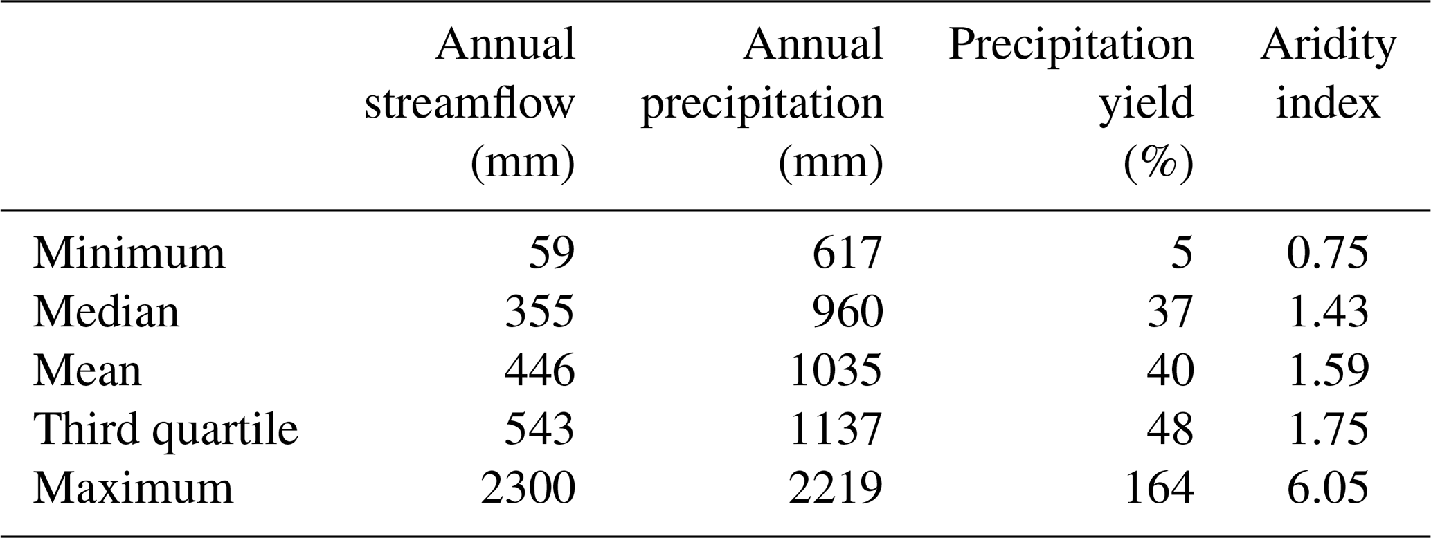
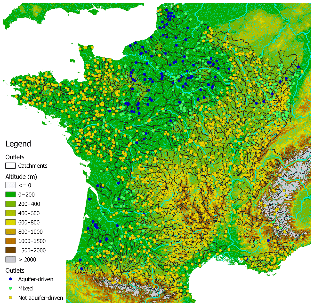
Figure 2Map of the catchments in the dataset. Dots represent the outlet of each catchment, with different colours according to the type of aquifer influence used in Fig. 8.
For each catchment of the dataset, a two-variable grid search was performed to find the optimum of the criterion. Hydrograph separation was then computed with the obtained parameters.
3.1 Criterion surface plots
As already mentioned in Sect. 2.2, for each catchment, there is a perfect bijection between values of the reservoir parameter S and values of the BFI: the BFI is a decreasing function of S. The BFI values are limited: in fact, when S tends toward infinity, the filter behaves like a minimum finder, and baseflow is constant, equal to the minimum flow; thus the BFI is always greater than Qmin∕Qavg, the ratio of minimum flow over mean flow. The BFI also has an upper bound, due to the numerical impossibility of getting a baseflow equal to total flow with the filter. Therefore, a range of possible BFIs was computed for each catchment, and the optimisation criterion can be seen as a function of the BFI and τ, defined for BFI values within this range. This function was then plotted on a contour plot to ensure a reasonable optimisation configuration.
Two examples of surface plots are presented in Figs. 3 and 4. The Vair River in Soulosse-sous-Saint-Élophe is a medium-sized basin dominated by impervious sedimentary formations. It is thus likely to have a low BFI value and response time. The criterion optimisation is unequivocal: the optimal point – which gives a correlation of 0.86 – has a difference greater than 0.15 with other local maxima. In agreement with geologic and climatic configurations, the optimised BFI (0.11) and τ (170 d) are low; the optimal value of S is 4.42 m. The Petit Thérain River in Saint-Omer-en-Chaussée is heavily influenced by the large chalk aquifer in the Paris basin: its BFI and response time should be high. The criterion optimisation is more equivocal here: there is a large plateau in the middle of the criterion map, around a correlation of 0.8, which gives significantly different values of BFI from 0.78 to 0.86 and τ from 700 to 1400 d. However, a hill in the middle of the shelf indicates the optimal point, where the correlation is 0.86, is at BFI = 0.783 and τ=1015 d. Pseudo-periodical oscillations can be seen in parallel to the τ axis; they are consequences of the annual hydroclimatic cycle.
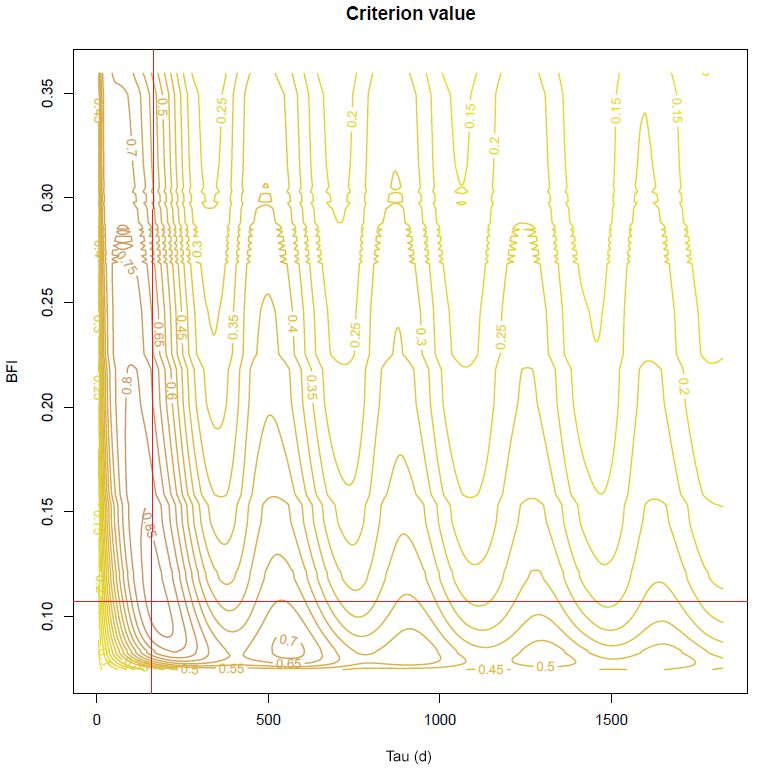
Figure 3Surface plot of the optimisation criterion for the Vair River in Soulosse-sous-Saint-Élophe. The red cross indicates the numerical optimum.
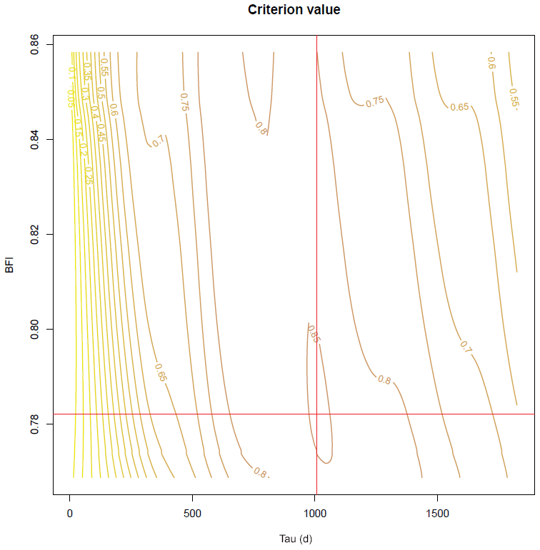
Figure 4Surface plot of the optimisation criterion for the Petit Thérain River in Saint-Omer-en-Chaussée. The red cross indicates the numerical optimum.
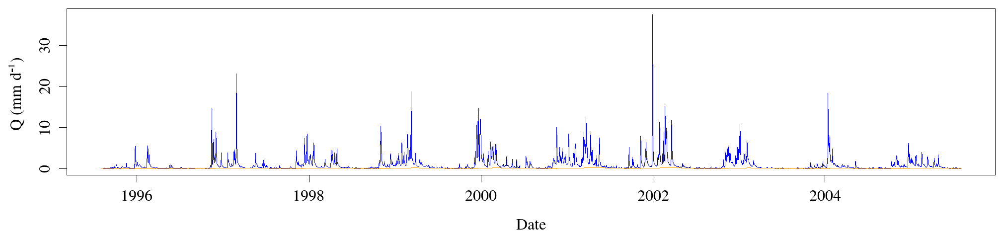
Figure 5Hydrograph separation of the Vair River in Soulosse-sous-Saint-Élophe for 1995–2005.
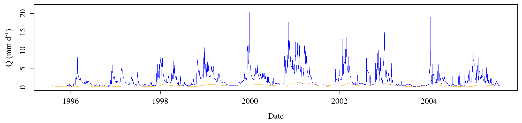
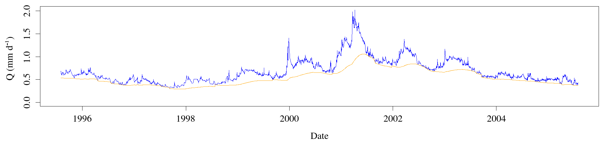
Figure 7Hydrograph separation of the Petit Thérain River in Saint-Omer-en-Chaussée for 1995–2005.
3.2 Hydrograph separations obtained
Figures 5–7 show three examples of hydrograph separations obtained among the test set of catchments, with the respective BFI values of 0.11, 0.30 and 0.78. Figure 5 shows the example for the Vair River in Soulosse-sous-Saint-Élophe, a small catchment in the Meuse basin, with a small BFI. It lies on poorly permeable sandstone, marl and clay, with no connection to a large aquifer. During dry periods, baseflow is almost determined by a local minimum on a sliding window with a length of 1 year, whereas it rises a little during wet periods, as seen during the 2000–2001 winter period.
Figure 6 displays a medium BFI case: the Virène River in Vire-Normandie is a granodioritic catchment located in the north-eastern part of the Armorican Massif, with a moderate aquifer influence. Baseflow fits the total flow during low-flow periods and rises during high flows, with a jagged shape made of asymmetric peaks: decreasing slopes fit the total flow, as a result of the update procedure, whereas increasing slopes are milder, driven by the smoothing effect of the reservoir. This creates a delay of baseflow with respect to total flow that resembles an aquifer's behaviour, with an outflow much higher just after a flood event than before. This baseflow recession resembles what would be obtained with a graphical separation method.
Figure 7 corresponds to a high-BFI case: the majority of flow is identified as baseflow by the model. The Petit Thérain River in Saint-Omer-en-Chaussée is a small catchment supplied by the well-known chalk aquifer of the Paris basin. Therefore, it is not surprising to find a BFI close to one. An ensemble view of the hydrograph shows that long oscillations seem to influence total flow, with a period greater than 1 decade; it is well taken into account by baseflow separation.
Among the dataset of 1664 catchments, optimisation of parameter S failed for three catchments only; there, the correlation criterion kept increasing with the value of S, without the possibility of reaching an optimal value. The failing catchments are small basins where most of the water comes from glaciers in the Alps: effective rainfall – as computed by the Turc–Mezentsev formula – is thus not really correlated with baseflow, and the quadratic reservoir fails to reproduce the particular memory effect of a glacier.
3.3 Synthesis and geological interpretation
Table 4 presents a summary of the parameters identified by calibrating the separation algorithm on the 1664 catchments. First, the obtained criterion values are quite high for Pearson correlations, with all values greater than 0.66 and half of the catchments above 0.80; baseflow is quite well-correlated with cumulated effective rainfall. Values of the reservoir parameter S are high compared with annual rainfall or with usual reservoir capacities for commonly used hydrological models; it is thus difficult to give them a physical meaning. The range of BFI obtained is large, between 0.01 and 0.90, with a median of 0.16. The chosen catchments represent a wide variety of situations that can be taken into account by the separation algorithm. Finally, τ also covers a wide range of values, between 5 and 1790 d, with half of the catchments between 165 and 200 d.
Table 4Summary of the results from the set of 1664 catchments.

We found that no clear relationship can be highlighted regarding the correlations between these results and hydroclimatic values given in Table 3. Therefore, no solution was found to reduce the number of parameters by inferring one from the other. However, a positive Pearson correlation of 0.42 between BFI and τ was found: catchments with higher baseflow have a larger response time, which is consistent with the conceptual definition of baseflow; the more important the slow component of streamflow is, the slower the average response of the system is.
Figure 8 shows the distribution of BFI and τ values for each hydrogeological class of basin. The mean BFI is significantly larger for aquifer-driven basins than for other classes, but the ranges of BFI are not significantly separated: even aquifer-driven catchments can have low BFIs. However, those that are not aquifer-driven are limited to BFI values under 0.4. This agrees with the fact that baseflow is highly connected to the outflow of aquifers, whose contribution to total flow is much higher in catchments connected to large underground reservoirs. There are also catchments whose geological configuration suggests an aquifer-driven regime, whereas the BFI found is low; most of them are located above the Vosges sandstone aquifer which, although a crucial resource for water supply in this region, is not directly connected to piedmont rivers. As far as τ is concerned, most catchments are around 200 d, with a larger mean value for aquifer-driven catchments. It is notable that mixed or not aquifer-driven basins are limited to values of τ less than 300 d, whereas the range of aquifer-driven catchments' values extends to more than 1000 d: this confirms the hypothesis that long memory is caused by the influence of an aquifer – even if the presence of the latter does not guarantee long-memory behaviour.
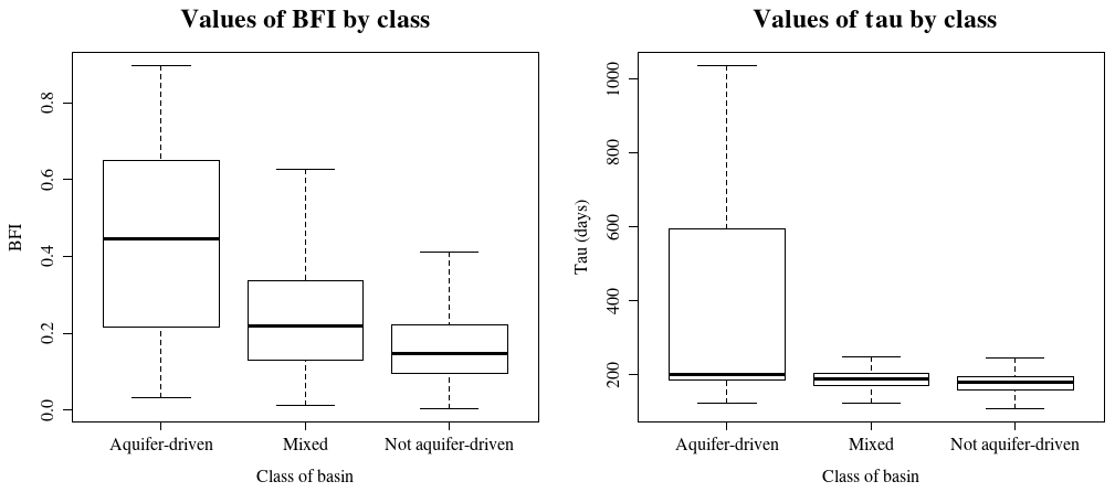
Figure 8Boxplots of BFI values and τ according to the hydrogeological class of basins, i.e. whether they are likely to be under the influence of a significant aquifer. Central box accounts for the interval between first and third quartile; the segment in the middle is the median; whiskers represent the 95 % confidence interval.
Figure 9 shows geographic variations of the obtained values of τ and BFI. BFI values are coherent with the geological context: granitic regions like the Armorican massif or Massif Central have low values of BFI; high values are observed in the Alsace plain, in the sandy Landes of Gascony, and particularly in the chalky zones of the Paris basin and the Somme basin. The rivers of these regions are known to be particularly under the influence of major aquifers that bear the memory of climatic events. The south-east area of France has medium BFI values, which is surprising, since most of this region is composed of mountainous areas without any large aquifers. However, particularly smooth hydrographs can be explained by the presence of many hydroelectric dams and natural lakes – the first of which is the Leman Lake on the Rhône River – in this region, which have a significant influence on streamflow. Values of τ are more difficult to interpret: even though the chalk aquifer is clearly visible around the Paris region, high values of τ can be observed in the Alps too, and medium values are found in the Massif Central. Here again, it can be explained by the presence of natural and artificial lakes that bear memory of past hydroclimatic events.
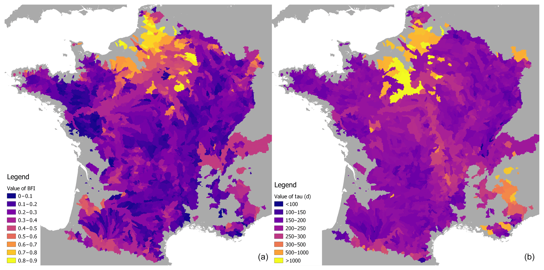
Figure 9Maps of resulting values of parameters on the catchment dataset. (a) BFI; (b) τ.
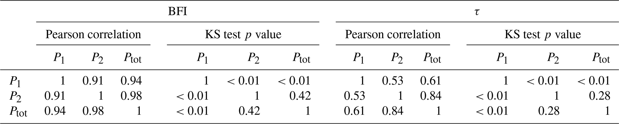
Table 5Statistical assessment of the split-sample test through Pearson correlation and the Kolmogorov–Smirnov (KS) non-parametric test.
3.4 Split-sample test as a stability assessment
In order to evaluate the stability of the proposed algorithm and of its calibration procedure, a split-sample test was performed. The time extent of the time series of the dataset – 1 August 1958 to 31 July 2018 – was divided into two equal periods P1 (1 August 1958 to 31 July 1988) and P2 (1 August 1988 to 31 July 2018). The algorithm was then calibrated separately for each basin on these two periods, and the values obtained for BFI and τ were then compared.
Figure 10 shows the graphical comparison of obtained BFI and τ values. Table 5 displays two statistical assessments that were performed after the split-sample test: correlation between values of BFI and τ and the non-parametric Kolmogorov–Smirnov test (Smirnov, 1939), in order to check the equality of distributions, i.e. the bias between series of values. The BFI shows a good graphical consistency, with high Pearson correlation values, higher than 0.91, but the p values of the Kolmogorov–Smirnov test are under 0.05 for P1; there is a constant bias between the BFI values computed for P1 and those computed for the whole period. The scatterplot shows a good correlation between the BFI values computed for P1 and P2. As for τ, it is less consistent than BFI: the scatterplot shows some outliers that are far from the diagonal, which explains the lower Pearson correlation values, between 0.53 and 0.84. Here again, values computed for P1 are further away from those computed for the whole period than those computed for P2. Despite these imperfections, this split-sample test can be regarded as successful, especially for a general-purpose analysis tool on a large set of catchments.
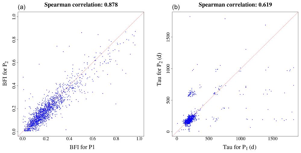
Figure 10Results of the split-sample test for BFI (a) and τ (b). Values obtained for P1 and P2 are compared.
3.5 Comparison with a reference method
The BFI obtained was compared with the one resulting from a simple graphical method, based on local minima on a sliding interval of 5 d. It is detailed in Gustard and Demuth (2008). Figure 11 shows the scatterplot of the two computed BFIs. Gustard's method gives higher indexes than the conceptual filtering algorithm, but the trend remains, which is confirmed by the high Spearman correlation: 0.819. A high-BFI catchment according to Gustard's method will also get a high BFI value from the conceptual filtering; low values follow the same pattern. The difference between the results of the two methods can be explained by the timescales: the width of the sliding minimum window in Gustard's method is 5 d, whereas we obtain much larger values of τ. Graphical quickflow is much quicker than the one resulting from the conceptual algorithm.
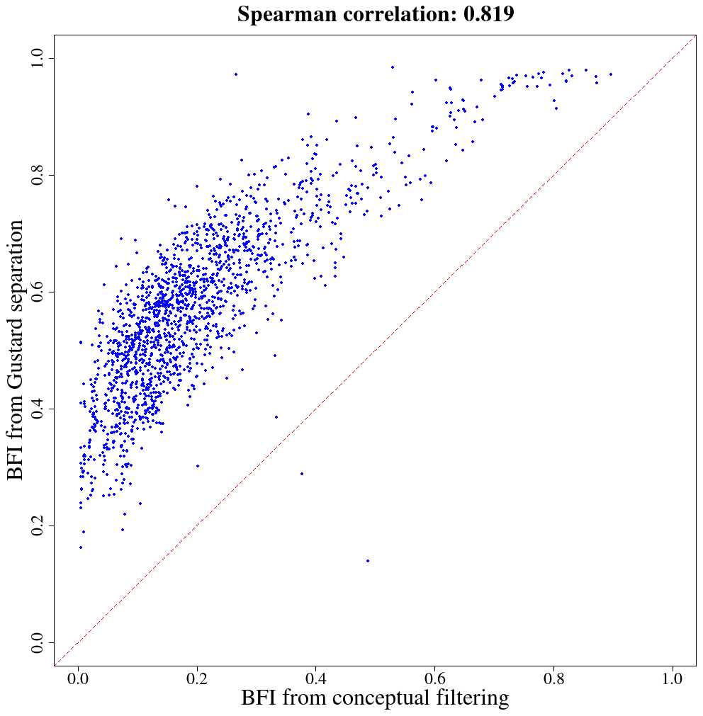
Figure 11Comparison between BFI obtained with the conceptual algorithm and a reference graphical method.
4.1 Synthesis
The hydrograph separation algorithm and its calibration procedure presented in this work have yielded credible results for a large set of test catchments. The algorithm has suitable characteristics for such a model: (i) frugality – only two parameters to calibrate; (ii) objectivity – the procedure is not supposed to require any intervention or interpretation from the user; (iii) generalisation ability – the procedure succeeded on the whole dataset, with a unique value found for the reservoir parameter; and (iv) repeatability – as assessed by the split-sample test performed on the test dataset. The analysis of the results in the light of the geological characteristics of catchments shows that the model is able to acknowledge the importance of groundwater flow in total flow generation without prior knowledge about the studied catchment, which is a significant step forward with respect to other non-tracer-based baseflow separation methods.
A conceptual and empirical baseflow separation method is neither intended to replace precise estimation of the elements of water balance at the scale of a given catchment, especially when in-field physical data are available nor can it precisely highlight particular hydrological processes occurring at the catchment or under-catchment scale, such as karstic non-linear transfers or human regulation of rivers. Yet, in the absence of in-field data, i.e. outside of specially instrumented catchments, conceptual baseflow separation is a useful tool for obtaining meaningful insights into the role of groundwater and aquifers inside a catchment. Even if the present method has limitations – which we summarise below – it could be applied as an objective, general-purpose, automated analysis tool for information on a large set of flow series. Beyond the inherent characteristics of the presented method, the results show that the hydrogeological processes of a catchment are deeply engraved in streamflow.
4.2 Limitations
We used an optimisation procedure set which searches for values of τ less than 5 years. It showed great convergence ability, i.e. an optimal point was found for every catchment of the test dataset. Yet, a mere glance at the Petit Thérain River hydrograph (Fig. 7) shows that its response time may be greater than 5 years, with long dynamics at the scale of climatic cycles. All this highlights the fact that the simplistic distinction between baseflow and quickflow hides the diversity of timescales and travel times among processes that influence the total flow of a river. Anyhow, the optimisation criterion is not indisputably univocal for a significant number of catchments; therefore, more work is needed to conceive a better optimisation criterion for the parametrisation strategy of the algorithm.
The split-sample test is a way to check temporal consistency of the baseflow separation method; the one performed on the test dataset can be considered as successful, at least concerning BFI results. Nevertheless, the spatial coherence of the method was not checked; it could be tested, for instance, with the propagation of baseflow sub-basins of a larger catchment, in order to test whether the sum of tributary baseflows makes up total baseflow. Our optimisation procedure does not take into account regional aspects while calibrating the model, although it could be a way of introducing objective prior knowledge into the method. On a sample of catchments where chemicophysical data are available, a comparison with tracer-based separation procedures would be a reliable way to validate the presented method.
Our algorithm is only intended for catchments that are not affected by human activity – pumping, regulation by dams or the use of canals – which excludes most large rivers in Europe. Finally, the generalisation capacity of the method has only been demonstrated for the hydroclimatic conditions of mainland France: even if the spatial extent of the present work has a substantial diversity of climates, a further study with a wider range of climates and geologies is needed to validate the method.
4.3 Implementation
An R package named baseflow (Pelletier et al., 2020) is provided to ensure the reproducibility of our results. It implements the algorithm presented in this paper with a high-performance computing core written in Rust. The example data taken from airGR are linked in the examples. The package is being released on CRAN (Comprehensive R Archive Network), and its documentation is available as supplementary material.
Data for this work were provided by Météo France (climatic data) and the hydrometric services of the French government (flow data). Flow data is publicly available on the Banque Hydro website http://hydro.eaufrance.fr/ (SCHAPI, 2015). Climatic data is not publicly available, since it is a commercial product; it can be freely provided – for research and non-profit purposes – upon request to Météo France.
The supplement related to this article is available online at: https://doi.org/10.5194/hess-24-1171-2020-supplement.
VA and AP conceptualised the method. AP performed the tests on the catchment dataset and developed the computing code. The paper was written by both authors.
The authors declare that they have no conflict of interest.
Data for this work were provided by Météo France (climatic data) and the hydrometric services of the French government (flow data). We would like to thank Pierre Nicolle (Université Gustave Eiffel) and Benoît Génot (INRAE Antony) for the database creation and maintenance and José Tunqui Neira (Sorbonne Université) for his help in the literature review. We would also like to extend our warmest thanks to Charles Perrin (INRAE Antony), Lionel Berthet (DGPR) and Paul Astagneau (INRAE Antony) for their remarks and suggestions during the writing process. Last but not least, computing codes could not have been developed without the precious expertise and availability of Olivier Delaigue (INRAE Antony) and Denis Merigoux (INRIA Paris).
This paper was edited by Markus Hrachowitz and reviewed by Renata Romanowicz and Ian Cartwright.
Bentura, P. L. F. and Michel, C.: Flood routing in a wide channel with a quadratic lag-and-route method, Hydrolog. Sci. J., 42, 169–189, https://doi.org/10.1080/02626669709492018, 1997. a, b
Beven, K.: Hydrograph separation?, in: Proc. BHS Third National Hydrology Symposium, Institute of hydrology, Southampton, UK, 3.2–3.8, 1991. a
Boussinesq, J.: Recherches théoriques sur l'écoulement des nappes d'eau infiltrées dans le sol et sur le débit des sources, Journal de Mathématiques Pures et Appliquées, 10, 5–78, 1904. a
Brodie, R. and Hosteletler, S.: A review of techniques for analysing baseflow from stream hydrographs, in: vol. 28, Proceedings of the NZHS-IAH-NZSSS 2005 conference, November 2005, Auckland, NZ, 2005. a
Cartwright, I. and Morgenstern, U.: Using tritium and other geochemical tracers to address the “old water paradox” in headwater catchments, J. Hydrol., 563, 13–21, https://doi.org/10.1016/j.jhydrol.2018.05.060, 2018. a
Cartwright, I., Gilfedder, B., and Hofmann, H.: Contrasts between estimates of baseflow help discern multiple sources of water contributing to rivers, Hydrol. Earth Syst. Sci., 18, 15–30, https://doi.org/10.5194/hess-18-15-2014, 2014. a, b
Chapman, T.: A comparison of algorithms for stream flow recession and baseflow separation, Hydrol. Process., 13, 701–714, https://doi.org/10.1002/(SICI)1099-1085(19990415)13:5<701::AID-HYP774>3.0.CO;2-2, 1999. a, b
Chow, V. T.: Runoff, in: Handbook of applied hydrology, McGraw-Hill, New York, USA, 1–54, 1964. a
Coron, L., Thirel, G., Delaigue, O., Perrin, C., and Andréassian, V.: The suite of lumped GR hydrological models in an R package, Environ. Model. Softw., 94, 166–171, https://doi.org/10.1016/j.envsoft.2017.05.002, 2017. a
Coron, L., Delaigue, O., Thirel, G., Perrin, C., and Michel, C.: airGR: Suite of GR Hydrological Models for Precipitation-Runoff Modelling, r package version 1.4.3.60, INRAE, Antony, France, https://doi.org/10.15454/EX11NA, 2020. a
Costelloe, J. F., Peterson, T. J., Halbert, K., Western, A. W., and McDonnell, J. J.: Groundwater surface mapping informs sources of catchment baseflow, Hydrol. Earth Syst. Sci., 19, 1599–1613, https://doi.org/10.5194/hess-19-1599-2015, 2015. a
Coutagne, A.: Les variations de débit en période non influencée par les précipitations – Le débit d'infiltration (corrélations fluviales internes) – 2e partie, La Houille Blanche, 5, 416–436, https://doi.org/10.1051/lhb/1948053, 1948. a, b, c
Delaigue, O., Génot, B., Bourgin, P.-Y., Brigode, P., and Lebecherel, L.: Base de données hydroclimatiqueà l'échelle de la France, Tech. rep., INRAE, UR HYCAR, Equipe Hydrologie des bassins versants, Antony, available at: https://webgr.inrae.fr/activites/base-de-donnees/ (last access: 9 March 2020), 2020. a
Duvert, C., Jourde, H., Raiber, M., and Cox, M. E.: Correlation and spectral analyses to assess the response of a shallow aquifer to low and high frequency rainfall fluctuations, J. Hydrol., 527, 894–907, https://doi.org/10.1016/j.jhydrol.2015.05.054, 2015. a
Eckhardt, K.: How to construct recursive digital filters for baseflow separation, Hydrol. Process., 19, 507–515, https://doi.org/10.1002/hyp.5675, 2005. a
Eckhardt, K.: A comparison of baseflow indices, which were calculated with seven different baseflow separation methods, J. Hydrol., 352, 168–173, https://doi.org/10.1016/j.jhydrol.2008.01.005, 2008. a
Fenicia, F., Kavetski, D., and Savenije, H. H. G.: Elements of a flexible approach for conceptual hydrological modeling: 1. Motivation and theoretical development, Water Resour. Res., 47, W11510, https://doi.org/10.1029/2010WR010174, 2011. a
Ficchì, A.: An adaptative hydrological model for multiple time-steps: diagnostics and improvements based of luxes consistency, PhD thesis, Université Pierre et Marie Curie, Paris, France, 2017. a
Gonzales, A. L., Nonner, J., Heijkers, J., and Uhlenbrook, S.: Comparison of different base flow separation methods in a lowland catchment, Hydrol. Earth Syst. Sci., 13, 2055–2068, https://doi.org/10.5194/hess-13-2055-2009, 2009. a, b, c
Gustard, A. and Demuth, S.: Manual on Low-Flow Estimation and Prediction, Tech. Rep. 50, World Meteorological Organization, Geneva, Switzerland, 2008. a
Habets, F., Gascoin, S., Korkmaz, S., Thiéry, D., Zribi, M., Amraoui, N., Carli, M., Ducharne, A., Leblois, E., Ledoux, E., Martin, E., Noilhan, J., Ottlé, C., and Viennot, P.: Multi-model comparison of a major flood in the groundwater-fed basin of the Somme River (France), Hydrol. Earth Syst. Sci., 14, 99–117, https://doi.org/10.5194/hess-14-99-2010, 2010. a
Hewlett, J. D. and Hibbert, A. R.: Factors affecting the response of small watersheds to precipitation in humid areas, Forest Hydrol., 1, 275–290, https://doi.org/10.1177/0309133309338118, 1967. a
Horton, R. E.: The Rôle of infiltration in the hydrologic cycle, Eos Trans. Am. Geophys. Union, 14, 446–460, https://doi.org/10.1029/TR014i001p00446, 1933. a
Jain, A., Sudheer, K. P., and Srinivasulu, S.: Identification of physical processes inherent in artificial neural network rainfall runoff models, Hydrol. Process., 18, 571–581, https://doi.org/10.1002/hyp.5502, 2004. a
Kirchner, J. W.: A double paradox in catchment hydrology and geochemistry, Hydrol. Process., 17, 871–874, https://doi.org/10.1002/hyp.5108, 2003. a
Kirchner, J. W.: Quantifying new water fractions and transit time distributions using ensemble hydrograph separation: theory and benchmark tests, Hydrol. Earth Syst. Sci., 23, 303–349, https://doi.org/10.5194/hess-23-303-2019, 2019. a
Klemeš, V.: Dilettantism in hydrology: Transition or destiny?, Water Resour. Res., 22, 177S–188S, https://doi.org/10.1029/WR022i09Sp0177S, 1986. a
Kronholm, S. C. and Capel, P. D.: A comparison of high-resolution specific conductance-based end-member mixing analysis and a graphical method for baseflow separation of four streams in hydrologically challenging agricultural watersheds, Hydrol. Process., 29, 2521–2533, https://doi.org/10.1002/hyp.10378, 2015. a
Labat, D.: Recent advances in wavelet analyses: Part 1. A review of concepts, J. Hydrol., 314, 275–288, https://doi.org/10.1016/j.jhydrol.2005.04.003, 2005. a
Leleu, I., Tonnelier, I., Puechberty, R., Gouin, P., Viquendi, I., Cobos, L., Foray, A., Baillon, M., and Ndima, P.-O.: La refonte du système d'information national pour la gestion et la miseà disposition des données hydrométriques, La Houille Blanche, 1, 25–32, https://doi.org/10.1051/lhb/2014004, 2014. a
Linsley, R. K., Kohler, M. A., and Paulhus, J. L. H.: Hydrology for engineers, 2nd Edn., McGraw-Hill, New York, available at: https://trove.nla.gov.au/work/13510461 (last access: 9 March 2020), 1975. a, b
Lott, D. A. and Stewart, M. T.: Base flow separation: A comparison of analytical and mass balance methods, J. Hydrol., 535, 525–533, https://doi.org/10.1016/j.jhydrol.2016.01.063, 2016. a
Maillet: Essais d'hydraulique souterraine & fluviale, A. Hermann, available at: http://archive.org/details/essaisdhydrauli00mailgoog (last access: 9 March 2020), 1905. a
Margat, J.: Carte hydrogéologique de la France: systèmes aquifères, Orléans, France, 1980. a
McDonnell, J.J. and Beven, K.: Debates – The future of hydrological sciences: A (common) path forward? A call to action aimed at understanding velocities, celerities and residence time distributions of the headwater hydrograph, Water Resour. Res., 50, 5342–5350, https://doi.org/10.1002/2013WR015141, 2014. a
Mei, Y. and Anagnostou, E. N.: A hydrograph separation method based on information from rainfall and runoff records, J. Hydrol., 523, 636–649, https://doi.org/10.1016/j.jhydrol.2015.01.083, 2015. a
Mezentsev, V.: Back to the computation of total evaporation, Meteorologia i Gidrologia, 5, 24–26, 1955. a
Michel, C., Perrin, C., and Andreassian, V.: The exponential store: a correct formulation for rainfall—runoff modelling, Hydrolog. Sci. J., 48, 109–124, https://doi.org/10.1623/hysj.48.1.109.43484, 2003. a
Miller, M. P., Johnson, H. M., Susong, D. D., and Wolock, D. M.: A new approach for continuous estimation of baseflow using discrete water quality data: Method description and comparison with baseflow estimates from two existing approaches, J. Hydrol., 522, 203–210, https://doi.org/10.1016/j.jhydrol.2014.12.039, 2015. a, b
Monteith, J. L.: Evaporation and environment, Symp. Soc. Exp. Biol., 19, 205–34, 1965. a
Oudin, L.: Recherche d'un modèle d'évapotranspiration potentielle pertinent comme entrée d'un modèle pluie-débit global, PhD Thesis, ENGREF (AgroParisTech), available at: https://pastel.archives-ouvertes.fr/pastel-00000931/document (last access: 9 March 2020), 2004. a
Oudin, L., Hervieu, F., Michel, C., Perrin, C., Andréassian, V., Anctil, F., and Loumagne, C.: Which potential evapotranspiration input for a lumped rainfall–runoff model: Part 2 – Towards a simple and efficient potential evapotranspiration model for rainfall–runoff modelling, J. Hydrol., 303, 290–306, https://doi.org/10.1016/j.jhydrol.2004.08.026, 2005. a
Pelletier, A., Andréassian, V., and Delaigue, O.: baseflow: Computes Hydrograph Separation, r package version 0.11.4, Antony, France, https://doi.org/10.15454/Z9IK5N, 2020. a
Perrin, C.: Vers une amélioration d'un modèle global pluie-débit au travers d'une approche comparative, La Houille Blanche, 6–7, 84–91, https://doi.org/10.1051/lhb/2002089, 2002. a
Perrin, C., Michel, C., and Andréassian, V.: Improvement of a parsimonious model for streamflow simulation, J. Hydrol., 279, 275–289, https://doi.org/10.1016/S0022-1694(03)00225-7, 2003. a
Pinault, J.-L., Amraoui, N., and Golaz, C.: Groundwater-induced flooding in macropore-dominated hydrological system in the context of climate changes, Water Resour. Res., 41, W05001, https://doi.org/10.1029/2004WR003169, 2005. a
Pinder, G. F. and Jones, J. F.: Determination of the ground-water component of peak discharge from the chemistry of total runoff, Water Resour. Res., 5, 438–445, https://doi.org/10.1029/WR005i002p00438, 1969. a
Réméniéras, G.: L'Hydrologie de l'ingénieur, Eyrolles, Paris, France, 1965. a
Roche, M.: Hydrologie de surface, Office de la recherche scientifique et technique outre-mer, Paris, France, 1963. a
Romanowicz, R.: An application of a log-transformed low-flow (LTLF) model to baseflow separation, Hydrolog. Sci. J., 55, 952–964, https://doi.org/10.1080/02626667.2010.505172, 2010. a
Saraiva Okello, A. M. L., Uhlenbrook, S., Jewitt, G. P., Masih, I., Riddell, E. S., and Van der Zaag, P.: Hydrograph separation using tracers and digital filters to quantify runoff components in a semi-arid mesoscale catchment, Hydrol. Process., 32, 1334–1350, https://doi.org/10.1002/hyp.11491, 2018. a
SCHAPI: Banque Hydro, available at: http://hydro.eaufrance.fr/ (last access: 9 March 2020), 2015. a, b
Singh, S. K., Pahlow, M., Booker, D. J., Shankar, U., and Chamorro, A.: Towards baseflow index characterisation at national scale in New Zealand, J. Hydrol., 568, 646–657, https://doi.org/10.1016/j.jhydrol.2018.11.025, 2019. a
Smirnov, N.: Estimate of deviation between empirical distribution functions in two independent samples, Bull. Moscow Univ., Moscow, Russia, 3–14, 1939. a
Su, C.-H., Costelloe, J. F., Peterson, T. J., and Western, A. W.: On the structural limitations of recursive digital filters for base flow estimation, Water Resour. Res., 52, 4745–4764, https://doi.org/10.1002/2015WR018067, 2016. a
Taormina, R., Chau, K.-W., and Sivakumar, B.: Neural network river forecasting through baseflow separation and binary-coded swarm optimization, J. Hydrol., 529, 1788–1797, https://doi.org/10.1016/j.jhydrol.2015.08.008, 2015. a
Turc, L.: Le Bilan d'eau des sols: relations entre les précipitations, l'évaporation et l'écoulement, PhD Thesis, Institut national de la recherche agronomique, Paris, 1953. a
Vidal, J.-P., Martin, E., Franchistéguy, L., Baillon, M., and Soubeyroux, J.-M.: A 50-year high-resolution atmospheric reanalysis over France with the Safran system, Int. J. Climatol., 30, 1627–1644, https://doi.org/10.1002/joc.2003, 2010. a
Wittenberg, H.: Nonlinear analysis of flow recession curves, in: FRIEND: flow regimes from international experimental and network data, vol. 221, IAHS Publications, Brunswick, 61–67, 1994. a, b, c
Wittenberg, H.: Baseflow recession and recharge as nonlinear storage processes, Hydrol. Process., 13, 715–726, https://doi.org/10.1002/(SICI)1099-1085(19990415)13:5<715::AID-HYP775>3.0.CO;2-N, 1999. a, b
Wittenberg, H. and Sivapalan, M.: Watershed groundwater balance estimation using streamflow recession analysis and baseflow separation, J. Hydrol., 219, 20–33, https://doi.org/10.1016/S0022-1694(99)00040-2, 1999. a