the Creative Commons Attribution 4.0 License.
the Creative Commons Attribution 4.0 License.
 | 07 Feb 2019
A conceptual model of organochlorine fate from a combined analysis of spatial and mid- to long-term trends of surface and ground water contamination in tropical areas (FWI)
Philippe Cattan
Jean-Baptiste Charlier
Florence Clostre
Philippe Letourmy
Luc Arnaud
Julie Gresser
Magalie Jannoyer
In this study, we investigated the management of long-term environmental pollution by organic pollutants such as organochlorine pesticides. We set out to identify conditions that are conducive to reducing pollution levels for these persistent molecules and then propose a conceptual model of organochlorine fate in water. Our approach looked at spatio-temporal changes in pollutant contents in surface water (SW) and groundwater (GW) on a large scale, in order to decipher the respective roles of soil, geology, hydrology and past treatment practices. The case of chlordecone (CLD) on the island of Martinique (1100 km2) was selected given the sampling campaigns carried out since 2007 over more than 150 sites. CLD, its metabolite chlordecone-5b-hydro (5bCLD) and the metabolite-to-parent-compound ratio were compared. As regards the spatial variability of water contamination, our results showed that banana cropping areas explained the location of contaminated SW and GW, whereas the combination of soil and geology factors explained the main spatial variability in the 5bCLD∕CLD ratio. For temporal variability, these conditions defined a high diversity of situations in terms of the duration of pollution, highlighting two groups: water draining old geological formations and ferralsols or vertisols vs. recent geology and andosols. A conceptual leaching model provided some key information to help interpret downward trends in CLD and 5bCLD observed in water. Lastly, a conceptual model of organochlorine fate is proposed to explain the diversity of the 5bCLD∕CLD ratio in water. Our conclusions highlight the combined role of soil and groundwater residence time for differentiating between conditions that are more conducive, or not, to the disappearance of CLD from the environment. This paper presents a model that provides an overall perception of organochlorine pesticide fate in the environment.
- Article
(5962 KB) - Full-text XML
- BibTeX
- EndNote


The pollution of rivers and aquifers by persistent organic pollutants (POPs) and organochlorine pesticides is a global issue (Gonzalez et al., 2012; Masih et al., 2014; Montuori et al., 2014; Zhang et al., 2004). Their long-term persistence after application (i.e. several decades to several centuries) raises the question of what is polluted and to what level, and how to manage and live with pollution. Moreover, the environment is not uniformly contaminated. Interactions between human pesticide application practices and environmental conditions lead to high variability in the contamination level of environmental compartments. This variability can be perceived by observing surface water (SW) and groundwater (GW) contamination.
Globally, changes in pesticide applications over several decades have resulted in downward and upward trends for pesticide concentrations in SW (Ryberg and Gilliom, 2015; Stone et al., 2014). This is also the case for GW, for which contamination trends have illustrated the leaching of pesticides from soils towards aquifers on a regional scale (Bexfield, 2008; Kolpin et al., 2004; Lapworth et al., 2006). Quality in SW is highly correlated to that in GW, due to strong interactions between aquifers and rivers on a watershed scale. Surprisingly, there is a lack of studies combining both SW and GW observations in order to characterise pollution in all the compartments (shallow and deep) of the hydrological cycle. Thus, this article addresses the issue of the conditions and processes that determine the spatial distribution of a persistent pollutant in water on a regional scale, investigating the case of chlordecone contamination in the French West Indies (FWI).
Chlordecone (CLD, C10Cl10O; CAS number 143-50-0; 491 g mol−1) is an organochlorine classified as a POP (US Environmental Protection Agency, 2012; UNEP, 2007). Numerous issues stem from CLD use in the French West Indies (islands of Martinique and Guadeloupe) (Lesueur Jannoyer et al., 2017). CLD was used from 1970 to 1993 to control the black weevil (Cosmopolites sordidus) in banana plantations. Application intensity greatly depended on the farmers (Cabidoche et al., 2009; Della Rossa et al., 2017; Levillain et al., 2012) and introduced high spatial variability in soil contamination. Despite its worldwide ban in 1992 (there was an exemption in FWI until 1993), CLD continues to contaminate aquatic ecosystems in different parts of the world (Coat et al., 2011; Luellen et al., 2006). As a consequence, CLD-polluted soils in FWI go on to contaminate GW (Arnaud et al., 2017; Gourcy et al., 2009) and rivers (Bocquene and Franco, 2005; Coat et al., 2011; Crabit et al., 2016; Mottes et al., 2015; Observatoire de l'Eau de la Martinique et al., 2012). This pollution raises concerns, as CLD causes adverse effects on health, from both acute and chronic exposure (Cannon et al., 1978; Cordier et al., 2017; Multigner et al., 2015).
The persistence of pesticides in soils and their transfer to percolation water depend on various processes, such as degradation and sorption, influenced by molecule properties, as well as the soil and climate context (Arias-Estévez et al., 2008). For CLD, adsorption on soil aggregates, and hence the risk of water pollution, greatly depends on soil type, as indicated by the soil organic carbon–water partitioning coefficient (Koc), which varies from 2.5 to 20 m3 kg−1 (Cabidoche et al., 2009; Woignier et al., 2012). Moreover, at depth, contrasting residence times (the water age in aquifers is defined as the mean transit time; Małoszewski and Zuber, 1982) in aquifers, ranging from several years to several decades, partly account for the variability in GW contamination by CLD (Gourcy et al., 2009).
Recent studies highlighted the fact that degradation can occur for this molecule (Fernández-Bayo et al., 2013; Mouvet et al., 2017). CLD-5b-hydro (5bCLD, C10Cl9HO; CAS number 53308-47-7; 456 g mol−1) is a mono-hydrochlordecone, which can be produced as an impurity during CLD manufacturing (Cabidoche et al., 2009; Fernández-Bayo et al., 2013). It has also been obtained experimentally by degradation of CLD through photolysis and microbial degradation (Orndorff and Colwell, 1980; Wilson and Zehr, 1979). Orndorff and Colwell (1980) interpreted the in situ value of 5bCLD content as an indicator of the degradation process. Studying the fate of both the parent and metabolite compounds, or their ratio, provides a more complete understanding of the transportation of the molecule (Farlin et al., 2017; Gassmann et al., 2013; Kolpin et al., 2004). 5bCLD has been found in soils, water and food webs, along with CLD, but at much lower levels (Borsetti and Roach, 1978; Clostre et al., 2015; Coat et al., 2011; Devault et al., 2016; Observatoire de l'Eau de la Martinique et al., 2012).
To sum up, in FWI human practices and the physical environment lead to high variability conditions for CLD and 5bCLD that may impact the environment. Our aim was to identify the conditions that are conducive to a decrease in pollution levels, in order to propose a conceptual model of organochlorine fate in water. We focus here on river contamination, which is driven by all the environmental compartments, thus being an integrative survey site for land use, soil variability and aquifer contributions. Based on the sampling campaigns in Martinique (FWI) since 2007, we explored river contamination trends over time and the relationships between surface and underground CLD rates in water. Spatial and temporal distributions of contamination were interpreted according to soil and geology mapping, hydrology, and past CLD treatment practices. This work will lead on to identifying areas with a low or high impact on water pollution, in order to manage polluted areas more effectively.

Figure 1Location (a) and relief (b) of the island of Martinique (FWI) in the Caribbean showing the banana cultivated areas.
2.1 Study site
2.1.1 Location and climate
The study area covered the volcanic island of Martinique (1100 km2) in the French West Indies in the Caribbean (Fig. 1). The climate is tropical, hot and humid. Annual rainfall is almost a linear function of altitude (0 to 1500 m a.s.l.) and ranges from 2500 to 10 000 mm on the east coast, and 1000 to 10 000 mm on the west coast.
2.1.2 Geology
Eight volcanic units (grouped into three simplified types according to the age of the volcanic arcs) have been identified (Germa et al., 2010, 2011) – see Fig. 3 for an overview of the geological map: (1) Basal Complex and Sainte Anne Series (24.8±0.4–20.8±0.4 Ma) for the older arc; (2) Vauclin–Pitault Chain (16.1±0.2–8.44±0.12 Ma) and (3) South-western Volcanism (9.18±0.16–7.10±0.10 Ma) for the intermediate arc; (4) Morne Jacob volcano (5.14±0.07–1.54±0.03 Ma), (5) Trois Ilets Volcanism (2.358±0.034 Ma and 346±27 ka), (6) Carbet Complex (998±14 to 322±6 ka), (7) Mount Conil (543±8 to 127±2 ka) and (8) Mount Pelée (126±2 ka to present) for the recent arc. The volcanism is andesitic with predominantly explosive volcanoes. Geological formations are thus composed by ash flows, lava flows and reworked formations (e.g. lahars and debris flows) channelled in peripheral valleys, and atmospheric fallout on a larger scale. Such geology generates a high spatial variability of lithology strata and contrasting weathering levels between geological units.
2.1.3 Soils
Two climate sequences of soils (IUSS Working Group WRB, 2014) are found in Martinique according to Colmet-Daage et al. (1965) – see Fig. 3 for an overview of the soil map: (1) ferralsols → nitisols → vertisols and (2) andosols → nitisols. All primary minerals of andesitic rocks are weathered, so that soils have a high content of secondary minerals: halloysite for nitisols, halloysite and Fe-oxihydroxides for ferralsols, and allophane for andosols. In addition, Martinique has skeletic andosols and young raw soil containing pumice gravels, deriving from recent pyroclasts. All these soil types are acidic. Carbon contents are unusually high for tropical soils, in particular for untilled andosols, and range from 10 to 140 g kg−1 according to Cabidoche et al. (2009) and Brunet et al. (2009). These features may induce large differences in pesticide fate in soils. Since the soil types “poorly developed soil on ash and pumice” and “andosol” are similar and rich in allophanes, in this study they were grouped under the designation “andosol”. Likewise, fersiallitic soils and ferralsols were grouped under the designation “ferralsol” (very dominant among the two soil types), as they are both rich in kaolinites (Colmet-Daage et al., 1965; Quantin et al., 1991).
2.1.4 Hydrology, hydrogeology and contamination
High rainfall intensities during tropical storms generate flash floods with a torrential regime in the rivers of Martinique. Permeable soils in the Lesser Antilles favour infiltration and aquifer recharge (Charlier et al., 2008). As a consequence, hydrological studies on a watershed scale showed that the water budget on an annual scale is mainly controlled by underground processes, limiting surface runoff contributions (Charlier et al., 2008, 2011). Stream flows are greatly influenced by SW–GW interactions, suggesting that GW drainage is a major process of river contamination (Arnaud et al., 2017; Charlier et al., 2009; Morgenstern et al., 2015; Mottes et al., 2015). At depth, most of the volcanic aquifers are small, a few square kilometres at most, as a result of the complex geological structure, which has undergone several phases of volcanism, erosion and weathering (Lachassagne et al., 2014; Vittecoq et al., 2015). As shown by Charlier et al. (2015), who compared the hydrogeological functioning of aquifers with contrasting lithologies and age formations, the groundwater residence time is highly variable, between a few years for recent unweathered formations (0.5–1 My) and several decades for old weathered formations (> 1 My). Given that the weathering of geological formations increases with their age, it is the main cause of a global decrease in aquifer permeability, notably in volcanic regions (Lachassagne et al., 2014). Indeed, clayey alteration products by weathering constrain the soil's physical and hydrodynamic properties by reducing porosity, and consequently permeability (Adelinet et al., 2008). It may result in various levels of river contamination by CLD linked to the hydrogeological context of the watershed.
2.2 Building up the database
2.2.1 CLD and 5bCLD sampling in water
The study period ran from the end of 2009–early 2010 to 2014. Since 2009–2010, 5bCLD has been analysed on a routine basis with CLD. For SW, we used data from a programme monitoring water quality carried out by the Martinique Water Office throughout Martinique and from a research programme implemented by CIRAD (CIRAD, 97285 Le Lamentin, Martinique, France) in the Galion watershed in Martinique. Sampling was carried out manually according to standard NF EN ISO 5667-3 and the FD T 90-523-1 guideline. For GW, we used data from a programme monitoring groundwater quality carried out by BRGM throughout Martinique. The sampling methodology was based on standard NF EN ISO 5667-3, and the FD T 90-523-3 and FD X31-615 guidelines. Before sampling in wells, at least three purge volumes were pumped with a submersible pump until stabilisation of the chemical groundwater parameters. Samples were stored at 5 ∘C and shipped in ice coolers to the BRGM analytical laboratory in Orléans, France.
2.2.2 CLD and 5bCLD analysis
5bCLD is the main alteration product of CLD (the term “alteration” here means that 5b is both a co-product and a degradation product) for which a commercial analytical standard is available. Reference standards for CLD and 5bCLD were purchased from Dr. Ehrenstorfer GmbH (Augsburg, Germany) for both laboratories with a purity degree of 96.7 %.
For SW, samples were analysed at the LDA26 laboratory. Analyses were carried out on raw sampling water. Thus, the water CLD and 5bCLD contents corresponded to dissolved and particulate fractions. It should be noted that the particulate fraction of the samples was low (< 250 mg L−1) due to sampling conducted mainly during periods of low flow. CLD and 5bCLD sample analyses were carried out by liquid ∕ liquid extraction (Dichloromethane and ethyl acetate 80∕20) followed by ultra-high-performance liquid chromatographic separation and mass spectrometric identification. An ultra-high-performance liquid chromatography tandem mass spectrometry analysis was performed with a Thermo electron system (TSQ Quantum Ultra) or ABSciex system (API4000 or API4000 Q-Trap). The compounds were separated on an Alltima C18 (5 µm; 150×2.1 mm. Two transitions were monitored 506.7 > 426.5 and 506.7 > 424.5 for CLD and 472.6 > 392 and 472.6 > 454.5 for 5bCLD. A 2.4D d3 was used as the internal standard for calibration. The key parameters of the method (linearity, repeatability, inter-day precision, specificity, extraction efficiency and limit of quantification) were validated in accordance with the NF T 90-210 standard method (AFNOR, 2009). The CLD and 5bCLD limits of quantification were determined by spiking natural surface water samples.
For GW, samples were analysed at the BRGM laboratory in Orléans, France. A gas chromatography tandem mass spectrometry analysis was carried out with a Bruker system (Marne la Vallée, France) composed of a GC450 gas chromatography apparatus equipped with a 1177 injector, a Combi Pal (CTC) autosampler and a 300MS triple quadrupole mass spectrometer. The injector was equipped with a 4 mm × 6.3 mm × 78.5 mm liner with fibreglass and Sky™ deactivation. The compounds were separated on an Rxi-1MS (30 m, 0.25 mm ID, 0.25 µm) column from Restek (Lisses, France). CLD and 5bCLD analyses of water samples were carried out by liquid/liquid extraction followed by gas chromatographic separation and mass spectrometric identification. The key parameters of the method (linearity, repeatability, inter-day precision, specificity, extraction efficiency and limit of quantification) were validated in accordance with the NF T 90-210 standard method (AFNOR, 2009). The CLD and 5bCLD limit of quantification were determined by spiking natural water samples.
Both the LDA26 and BRGM laboratories are accredited for pesticide analysis and are involved in proficiency testing schemes organised by ANSES (French Agency for Food, Environmental and Occupational Health, and Safety), thereby ensuring the quality and coherence of the results. The limits of CLD and 5bCLD quantification in water were different for LDA26 and BRGM: 0.01 and 0.03 µg L−1, respectively. By convention, the limits of detection were set at one-third of the limits of quantification, i.e. 0.003 and 0.01 µg L−1 for LDA26 and BRGM, respectively.
2.2.3 Value assessment and factors
Value assessment
For calculation, a value of 10 % of the quantification limit was assigned when the compound was not detected (i.e. 0.001 for LDA26 or 0.003 µg L−1 for BRGM), and an intermediate value of 0.006 µg L−1 was assigned when the compound was detected but not quantifiable at LDA26.
Factors
The statistical analysis set out to assess the effect of various environmental factors – soils, geology, hydrological sectors, historical banana cultivation areas and time – on CLD and 5bCLD concentrations and on the 5bCLD∕CLD ratio, determined at each sampling point. For the soil factor, as the water at one sampling site originated from a watershed possibly draining various soil types, we associated each sampling point with the main soil type of the watershed drained by the sampling point according to the soil map of Colmet-Daage et al. (1965). For the other factors, each sampling point was associated with the factor value at the sampling point.
2.3 Selection of data and statistical analysis
2.3.1 Range of contamination values
The relevance of contamination was assessed according to the EU “Water Framework” and “Quality of drinking water” Directives (European Union, 1998, 2000) and their transposition into French law (French government, 2001). Three thresholds of water contamination classes stemmed from these directives: 0.1, 0.5 and 2.0 µg L−1. The first two regulatory thresholds apply to the mean annual content in tap water intended for human consumption: 0.1 µg L−1 is the threshold for each pesticide (threshold applying to CLD), and 0.5 µg L−1 is the threshold for the sum of all pesticides. Raw water exceeding these thresholds needs to be treated for human consumption. The third value, 2.0 µg L−1, is the threshold beyond which, according to the regulation, water can no longer be termed drinkable even after treatment. The threshold values of 0.1 and 0.5 µg L−1 are also chosen to define good environmental status.
2.3.2 Data selection
Global data set
For SW, the data set consisted of 1866 analyses from 136 sampling points and 76 rivers. The analyses were not evenly distributed. Most of the sampling points had a low measurement frequency (105 had fewer than 5 analyses) and only 18 sampling points had more than 50 analyses covering the entire 2009–2014 period. However, the number of analyses per complete year varied between 188 and 352. For GW, the data set consisted of 282 analyses from 21 sampling points and 6 water bodies. Basically, sampling occurred twice a year at each sampling point. At three sampling points, sampling occurred monthly in some years.
Data selection for statistical models
For statistical analysis, we discarded data where CLD concentrations were below detection limits (and consequently 5bCLD concentrations too, as 5bCLD concentrations are always lower than CLD), as they would have led to an inappropriate ratio value (ratio of 1 according to the value assessment rule described below). Additionally, although we gathered data from contaminated areas, some of the water samples were contaminated with CLD, but no 5bCLD was detectable. For the statistical analysis, we kept all the data (with and without quantifiable 5bCLD) from sampling points for which at least half the samples had quantifiable 5bCLD contents (≥0.03 or 0.01 µg L−1). This avoided overestimating the concentration for the sampling point, which would have been the case if we had discarded all the data with no quantifiable 5bCLD. For SW, we selected 963 data items (i.e. water samples analysed for CLD and 5bCLD). This SW data set covered 38 sampling points out of a total of 136. For GW, we selected 123 data items. This GW data set came from 7 sampling points.
Data selection for temporal analysis on specific rivers
In order to highlight differences between pesticide trends depending on the sampling point, we chose rivers for which the analysis covered the entire 2009–2014 period. This led to the selection of 14 sampling points, all with more than 50 analyses. As stated above, we discarded analyses where CLD and 5bCLD contents were below detection limits.
2.3.3 Statistical analysis
Models
To ensure that the residue distribution of the analysis of variance (ANOVA) model followed the assumptions of equal variance and normality, we used log transformed (natural log) data. We analysed our SW and GW data sets by a multi-way analysis of variance using the MIXED procedure in SAS software (SAS Institute Inc, 2002). The effects to be taken into account in the models were chosen by comparison with the AIC (Akaike Information Criterion).
Model 1 was used on the SW data set to test different effects on the CLD content, the 5bCLD content and the ratio of the 5bCLD content to the CLD content in SW. The soil and geology factors were dependent on each other. For this reason, only combinations of these two factors were considered in the model.
where Yijklm is the observation (i.e. ln(5bCLD), ln(CLD) or ln(5bCLD∕CLD)), μ is the general mean, αi is the (soil × geology) type effect, βij the hydrological sector effect for each (soil × geology) type, γt is the date effect, Dijk the random effect of the sampling point for each (soil × geology) type and εijtkl is the residual error. Indices i, j, t, k, l represent the factors for soil × geology, hydrological sector, date, sampling point and sample replication, respectively.
Model 2 was used on the GW data set. Soil and geological factors were closely linked for the GW data set (andosols were always associated with recent geological formations and ferralsols with old geological formations), making it impossible to distinguish the soil effect from geology; likewise for groundwater basins and hydrographic sectors. Consequently, only soil and hydrographic sectors were tested for model 2:
where is the observation (i.e. ln(5bCLD), ln(CLD) or ln(5bCLD∕CLD)), μ′ is the general mean, α'i is the soil type effect, β'ij the hydrological sector effect for each soil, the date effect, the random effect of the sampling point for each soil and is the residual error. Indices i, j, t, k, l represent the factors for soil, hydrological sector, date, sampling point and sample replication, respectively.
The significance of the sampling point effect was assessed by comparison of −2 log likelihood from the models with and without the sampling point as the random effect, as this difference followed a chi-square distribution under the null hypothesis.
Trend analysis
For SW, to study temporal trends, we selected estimated means of the time series for each date. Autocorrelations were assessed with the Durbin–Watson test and monotonic trends were assessed with the Mann–Kendall (MK) test. We calculated Sen trends (Sen's slope estimator, Gilbert, 1987) for each variable (CLD, 5bCLD and ratio) in order to compare dynamics for the two compounds. The Sen trend of a set of two-dimensional points (xi,yi) and (xj,yj) is the median of the slopes () determined by all pairs of sample points. The Sen trend is more robust than the least-squares estimator, because it is much less sensitive to outliers.
2.3.4 Conceptual model of CLD fate
A simple iterative leaching model was developed to assess the evolution of
CLD, 5bCLD and the 5bCLD∕CLD ratio over time. This model expressed that
the 5bCLD∕CLD ratio in water depended equally on degradation and transfer
rates as well as the remaining storage of CLD and 5bCLD in soils. The
governing equations are given below:
CLD storage in soil:
5bCLD storage in soil:
Ratio in water:
TCLD and T5bCLD are the rates of lixiviation for CLD and 5bCLD (i.e. the ratio of lixiviated mass of CLD or 5bCLD to their respective mass in soil), respectively; Cdegrad is the rate of CLD degradation into 5bCLD; C5bdegrad is the rate of 5bCLD degradation; and t is the time. CLD and 5bCLD are expressed in units of mass. According to data reported by Cabidoche et al. (2009), considering an area of 1 m2 and that pollutants are distributed within the first 3 dm of soil, TCLD is expressed as follows:
where Koc (L kg−1) is the partitioning coefficient between the sorbed part on soil organic matter and the dissolved part in water, D (kg dm−3) is the bulk density, C (g kg−1) is the soil carbon content, R (dm) is the annual amount of rainfall, S is the soil surface area (dm2) and d is the soil depth (dm).
The calculation steps are given below:
-
the setting of the initial CLD and 5bCLD stocks to 100 and 0 units of mass respectively;
-
calculation of leached CLD quantities (Eq. 3);
-
calculation of degraded CLD quantities, i.e. transformed in 5bCLD (Eq. 3);
-
calculation of remaining CLD quantities (Eq. 3);
-
calculation of leached 5bCLD quantities (Eq. 4);
-
calculation of degraded 5bCLD quantities (Eq. 4);
-
calculation of remaining 5bCLD quantities (Eq. 4);
-
calculation of mass ratio in water (Eq. 5), which accounts for the concentration ratio since the two compounds are leached with the same water quantities.
3.1 Variability of CLD contamination and its relationships with 5bCLD
Figure 2 shows the relationship between the means of 5bCLD and CLD in rivers at each sampling point. We found that the water 5bCLD content was at least 10 times lower than the water CLD content. However, there was not a unique relationship between 5bCLD and CLD. The frequency distribution of the means of the 5bCLD to CLD ratio in SW and GW clearly showed that a threshold of 0.07 divided the data set into two groups: a low and a high ratio around 0.02 and 0.1, respectively. According to Devault et al. (2016), these differences cannot stem from the use of different commercial products or different batches of the same product. Indeed, these authors found no significant statistical difference between the ratio of the commercial products Kepone® and Curlone® used in FWI, no more than they did between samples from different batches of Curlone®. They found a mean ratio in commercial products of 0.00077±0.00027, i.e. 10 times lower than our observations in river.
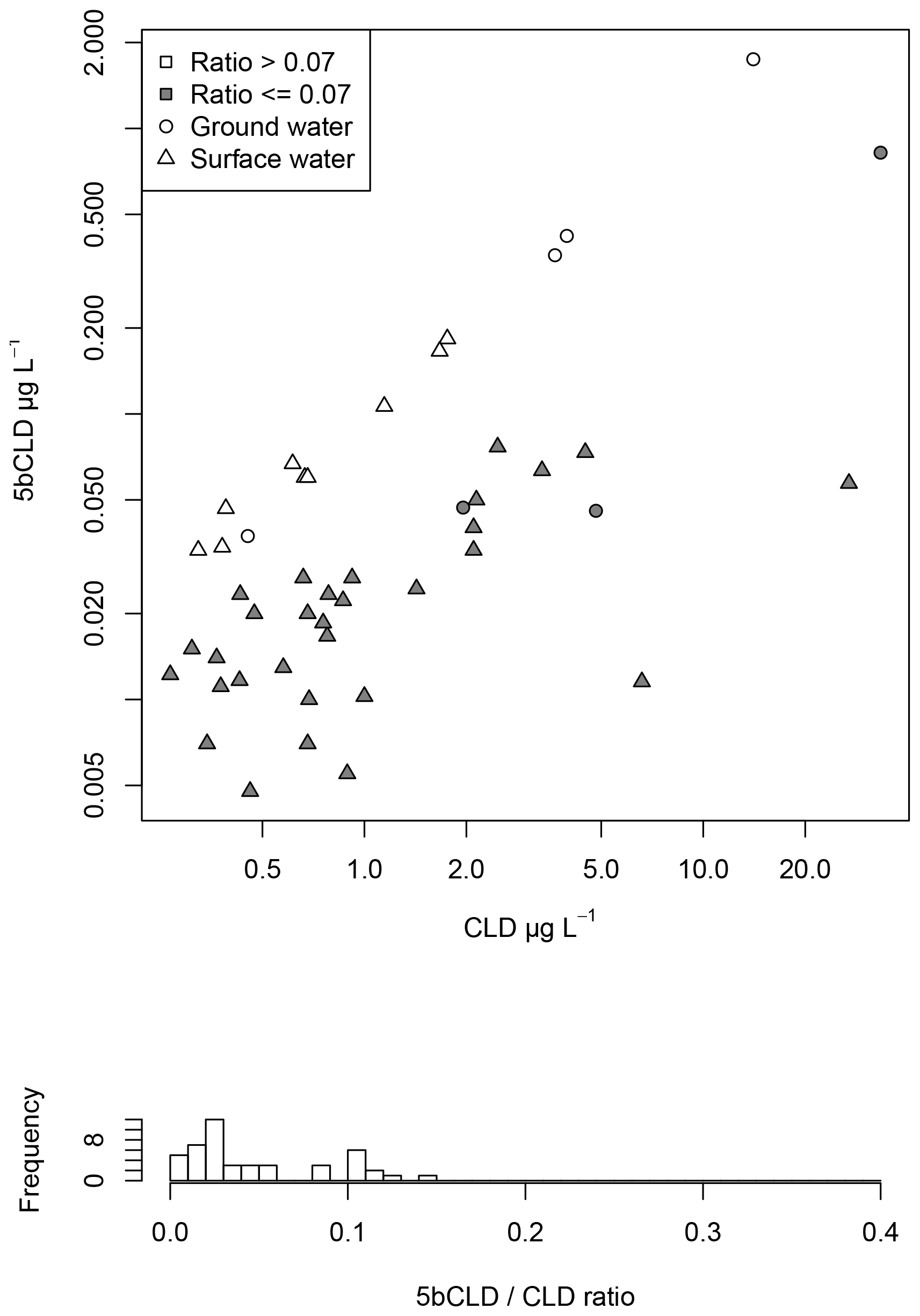
Figure 2Relation between CLD and 5bCLD means at each sampling point for surface water and groundwater; distributions of the mean of the 5bCLD∕CLD ratio are given below the 2-D plot.
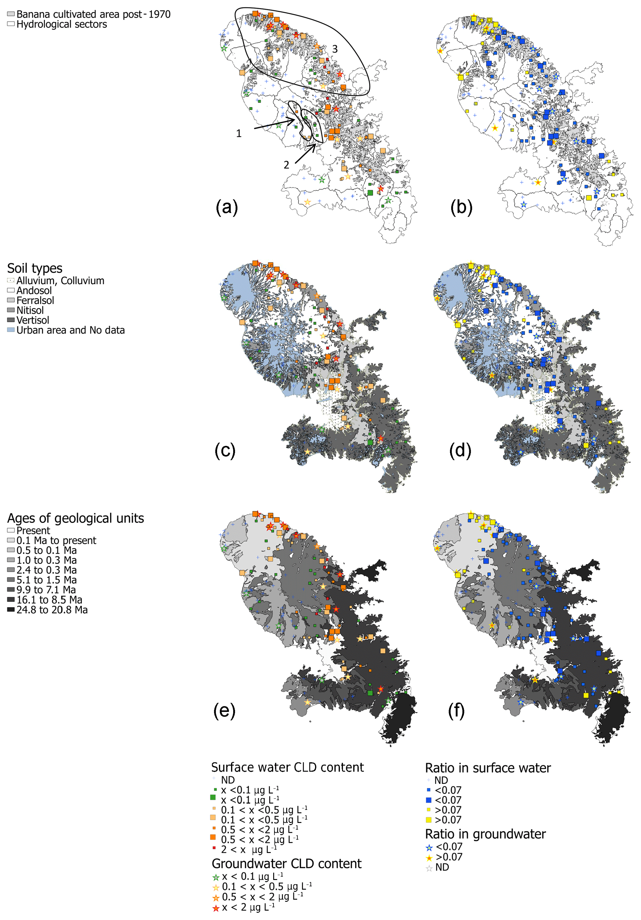
Figure 3Distribution of water CLD content (a, c, e) and the 5bCLD∕CLD ratio (b, d, f) for surface water (square) and groundwater (star), according to banana cultivated areas and hydrological sectors (a, b), soils (c, d) adapted from Colmet Daage (1965), and geology (e, f) adapted from Germa et al. (2011). Large squares are relative to sample points with more than 10 sampling dates and small squares to those with fewer than 10 sampling dates.
3.2 Spatial analysis
3.2.1 General distribution
Figure 3 presents the CLD concentrations (top) and the 5bCLD∕CLD ratio (bottom) for SW (square/triangle) and GW (star) throughout Martinique, according to hydrological sectors (left), soil (middle) and geology. The top of Fig. 3 shows that the most challenging areas relative to CLD contamination were mainly situated in the northern Atlantic and central part of Martinique. The distribution for the 5bCLD∕CLD ratio was different. The bottom of Fig. 3 shows that the group with the high ratio (> 0.07) was mainly located either in the highly contaminated northern areas, or in some parts of the low-contamination areas in southern and western Martinique.
We observed overall consistency between the distribution of SW and GW contamination: the higher the CLD content or 5bCLD∕CLD ratio for SW, the higher the CLD content or 5bCLD∕CLD ratio for GW. However, the west coast displayed some exceptions, since we observed contaminated GW (primarily low contamination) while CLD was not detected in the rivers in the neighbourhood. Similarly, the 5bCLD∕CLD ratio for GW belonged to the high value group (> 0.07 µg L−1), while the 5bCLD∕CLD ratio for SW belonged to the low value group, or was not available because of the lack of contamination.
3.2.2 Impact of physical conditions
Land-use practices: high level of contamination in historical banana cultivation areas
Globally, for the water CLD content, the SW and GW contamination sites matched with the historical banana cultivation areas since 1970, i.e. during CLD application. Surprisingly, SW and GW contamination occurred outside these banana cultivation areas. This was mostly with low concentrations under 0.1 µg L−1 and rarely with the higher levels (one point in the south-west for GW, far from the banana cultivation area). Most of these isolated points had a high 5bCLD∕CLD ratio, leading the 5bCLD∕CLD ratio not to match banana field distribution, suggesting past CLD misuse.
Table 1Effects of physical conditions on the contamination level of surface water (model 1) and groundwater (model 2), showing probability levels of tested factors. Bold: statistically significant at the 0.05 probability level. Italics: statistically significant at the 0.10 probability level.

Hydrographic sector: a functional relationship between measurement points
Introducing hydrographic subsectors made it possible to establish a functional relationship between measurement point data. Notably, this helped to explain why some points close to each other did not have the same contamination level. For example, although sample points of subsector 1 and 2 were very close (see Fig. 3a), they did not have the same contamination level. In contrast, all the sample points of subsector 1 had the same contamination level (same for subsector 2). This suggests that the hydrographic sector, i.e. the water flows within the same hydrological unit, mainly determined the contamination level of the sample points, rather than the geographical closeness of those points. However, some differences were found on the north-east coast. This was encountered in zone 3, where the contamination levels seemed to be linked to the altitudinal gradient. Contamination increased downwards in coherence with banana field distribution along the coast at the lowest altitudes. The statistical results summarised in Table 1 confirm this interaction between hydrographic sectors and soil/geology for CLD and GW. However, no effect was found for the 5bCLD content and the 5bCLD∕CLD ratio.
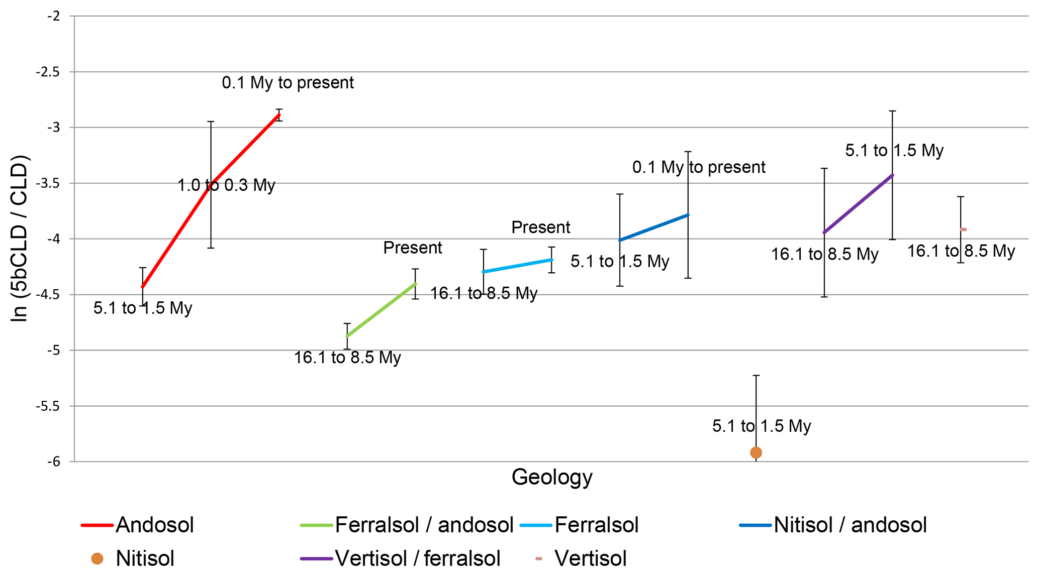
Figure 4Mean 5bCLD∕CLD ratio (natural logarithm) according to soil types and to the age of the geological formations. Ferr_And, Nit_And and Vert_Ferr account for watersheds with two main types of soil, namely ferralsols and andosols, nitisols and andosols, and vertisols and ferralsols. The y values of −6, −4 and −2 correspond to ratio values of 0.002, 0.018 and 0.135, respectively.
Soil type: a factor explaining some ratio variations in SW
Table 1 shows significant differences in GW CLD contamination according to the soil/geology pair: GW on nitisols, which are associated with old formations (older than 1 My), was more contaminated than on andosols associated with recent formations (1 My to present). This did not result in any significant difference for SW. However, for SW, we observed significant differences for the 5bCLD∕CLD ratio, opposing a low ratio for nitisols to a higher ratio for andosols (Fig. 4). We also noted a higher ratio for vertisols. This is statistical confirmation of the result mapped in Fig. 3, showing high 5bCLD∕CLD ratios on vertisols in southern Martinique.
Geology: a factor explaining ratio variations in SW and GW
The age of the main geological units was used as an indicator of hydrogeology, and notably residence time in the aquifers, which is linked to pesticide transfer kinetics in GW, as well as in SW fed by it. Therefore, shorter residence times were observed for aquifers located in more recent and unweathered geological formations. It can be seen in Fig. 3 that the highest CLD contents in water matched with recent geological formations in the banana cropping area (northern half of the island). Medium and low CLD contents were observed in other older geological units, or outside banana cropping areas. As regards the 5bCLD∕CLD ratio, the highest values were only observed in the most recent units (0.5 My to present), for the most contaminated water bodies in the North Atlantic area (not shown).
It is interesting to note that the soil effect depended on geology. Figure 4 illustrates this, presenting the mean ratio for each soil type according to the age of the geological formations. For andosols and ferralsols/andosols, the ratio appeared to be significantly higher for recent geology.
To sum up, banana cropping areas explained the location of contaminated SW and GW, whereas the combination of soil and geology factors explained the main spatial variability of the 5bCLD∕CLD ratio, with the highest values in the north associated with recent geological units and the highest values in the south associated with vertisols.
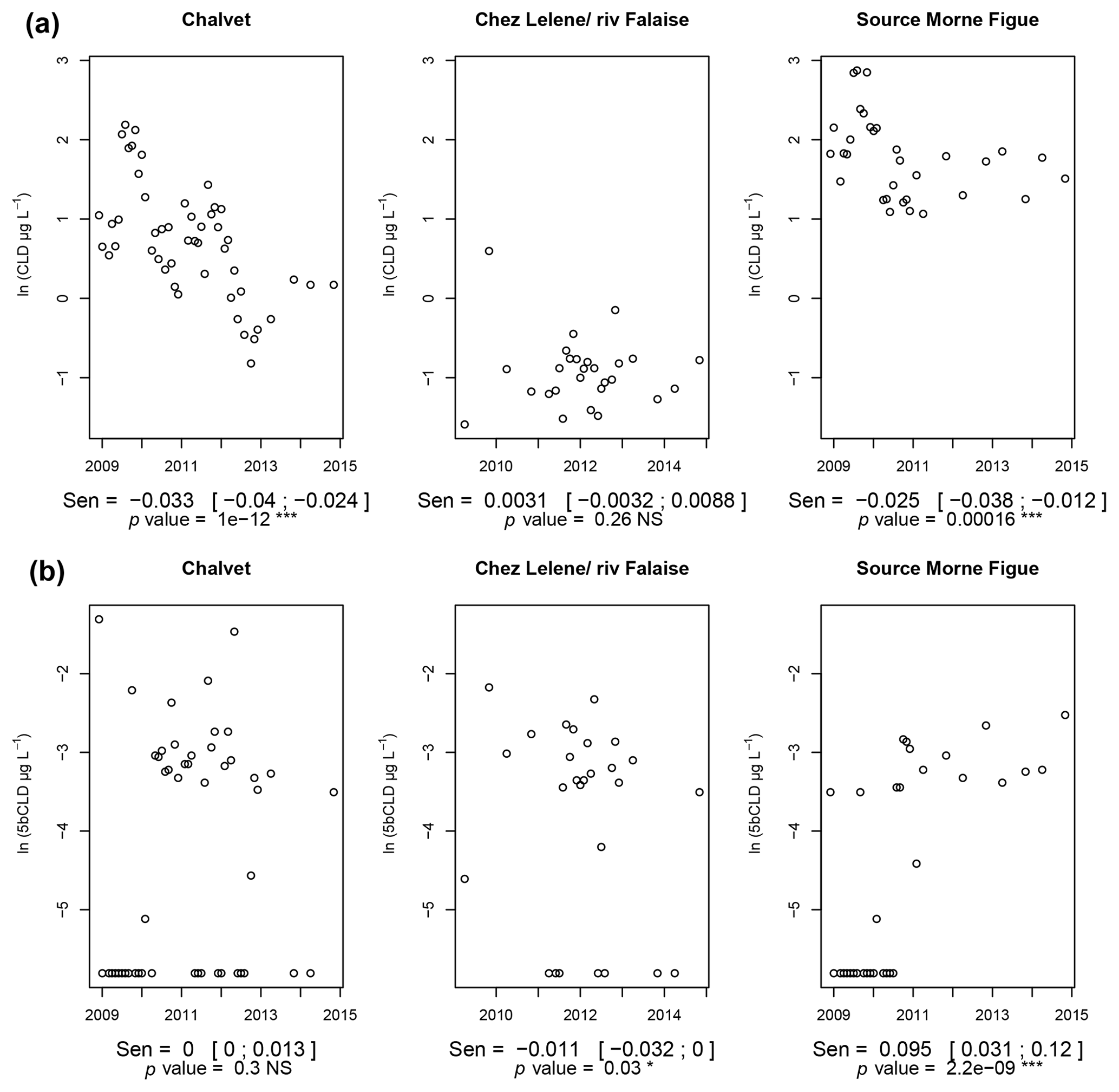
Figure 5CLD (a) and 5bCLD (b) trends in GW for the three longest time series (the y scale is in natural logarithm). Soil and geology are andosol and 0.1 My to present for the Chalvet and Chez Lelene sites and nitisol and 16.1 to 8.5 My for the Source Morne Figue site. Sen trends and p values show a significant CLD decrease for Chalvet and Source Morne Figue. We found 5bCLD decreased at Chez Lelene while it increased at Source Morne Figue.
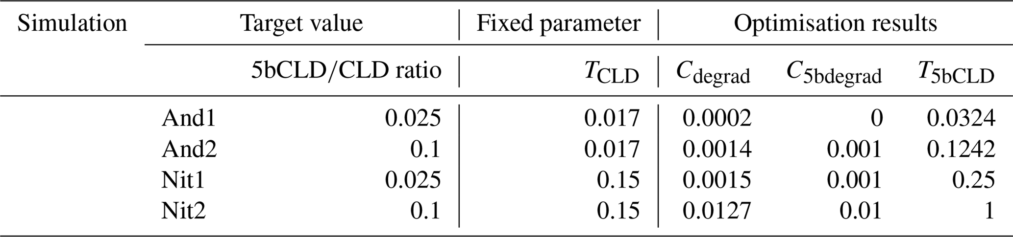
Table 2Parameters of four simulation scenarios for CLD and 5b CLD fate. CLD and 5bCLD degradation rate (Cdegrad C5bdegrad) and 5bCLD lixiviation rate (T5bCLD) stemmed from optimisation processes based on two target values of the 5bCLD∕CLD ratio in leaching water (cases 1 and 2), as well as two hypotheses for the CLD (TCLD) lixiviation rate (fixed parameter) corresponding to andosol type (And) and nitisol type (Nit).
3.3 Temporal analysis
3.3.1 Pesticides evolve differently in GW
Figure 5 illustrates pesticide trends in GW for the three longest available time series. The mean CLD content decreased globally for two sites (Chalvet and Source Morne Figue) and remained stable for Lelene, while the 5bCLD content had a more erratic evolution, probably due to the greater influence of hydrological conditions (climatic seasonality). As pointed out by Arnaud et al. (2016), these contamination periods correspond to rising and falling groundwater levels, and therefore to periods of aquifer recharge. For the two sites showing a decrease in water CLD content, the number of samples with 5bCLD contents below the detection limit decreased over time, and equalled zero in the case of the Source Morne Figue site after 2011. This was consistent with an increase in 5bCLD content, or at least with a more regular occurrence of positive values. Lastly, despite the impossibility of generalising behaviour with the limited sampling sites and available period series, the groundwater data sets showed an interesting evolution pattern with, in some cases, a decrease in CLD content associated with an increase in water 5bCLD content.
3.3.2 In SW: the pesticide concentration and ratio globally decreased
From all the available data, we observed a highly significant downward trend in mean river concentrations for the CLD content, 5bCLD content and the 5bCLD∕CLD ratio in water (a slope of −0.008, −0.028 and −0.018, respectively). It is interesting to note that the decreasing trend for the 5bCLD content was about three times higher than for the water CLD content.

Figure 6CLD (natural logarithm) trends in SW according to geology and soil type. Sen trend and confidence interval; p value of the modified Mann–Kendall test for serially correlated data using the Yue and Wang variance correction approach. CLD content significantly decreased (p value < 0.05) for 10 out of 14 rivers. Thick lines (Pont RN1 and AEP-Vive-Capot) indicate a large decrease (lower than percentile 0.1 of Sen trends); thin lines (Camping Macouba and Saint Pierre) indicate a small decrease (higher than percentile 0.9).
More specifically, Fig. 6 shows the evolution of water CLD content for the 14 rivers with the highest measurement frequency. Globally, the mean Sen trend was −0.008 for the log, meaning that the CLD content was halved after 7.5 years. Although most of the rivers showed a significant decrease in water CLD content, some of them were characterised by a constant level of contamination (Saint Pierre, Pont RN Rouge) and one even showed a slight increase (Camping Macouba). Independently, we noted a high variation in the level of contamination.
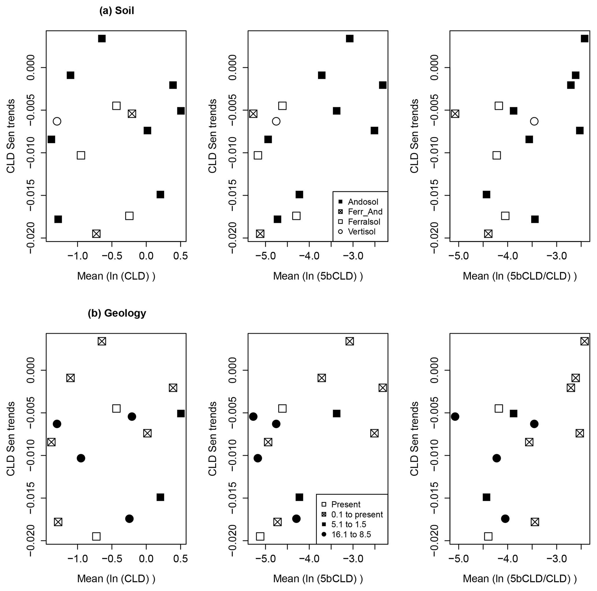
Figure 7Sen trends of CLD vs. mean log content of CLD, 5bCLD and 5bCLD∕CLD ratio (from left to right – natural logarithm) in SW, according to (a) soil and (b) geology (for soil and geology, see legend in the middle figure).
A further analysis of temporal evolution (Fig. 7) highlighted a relationship between Sen trends for CLD and the mean water 5bCLD contents (regression p value =0.06): the lower the water 5bCLD content, the greater the decrease in water CLD content. A similar trend was observed for the 5bCLD∕CLD ratio (regression p value =0.05), while the relationship was not significant for mean water CLD content. This indicated that the decrease intensity did not depend on water CLD content. Figure 7a and b (left: Sen CLD vs. mean CLD) shows favourable situations at the bottom left, where strong decreases in water CLD content were associated with a low water CLD content in SW, which gives hope for pollution mitigation. Adversely, in the situations at the top right of the figure, the pollution level is likely to last for a long time.
Additionally, Fig. 7b shows that the smallest decreases in water CLD content were partly associated with recent (0.1 My to present) geological formations and that the largest decreases were associated with older ones. Lastly, regarding soils, Fig. 7a shows that while andosols were distributed over the entire range of Sen trends, ferralsols and vertisols characterised large decreases in water CLD content.
To sum up, high water CLD contents decreased with low water 5bCLD contents and low 5bCLD∕CLD ratios were encountered for basins situated on old geological formations and mostly ferralsols or vertisols. On andosols and recent geological formations, the water CLD content did not vary over the study period, and the water 5bCLD content and 5bCLD∕CLD ratio were high. These conditions define a high diversity of situations with regard to the persistence of pollution.
3.4 Model simulation
In order to grasp the complex fate of CLD and 5bCLD, we used the simple model presented in Sect. 2.3.4. It is an iterative leaching model investigating the theoretical fate of CLD and 5bCLD in water, accounting for CLD and 5bCLD lixiviation rates (TCLD and T5bCLD), as well as the rate of CLD degradation into 5bCLD (Cdegrad). Table 2 gives the results of the optimisation processes in order to assess T5bCLD, Cdegrad and C5bdegrad from realistic values of TCLD and the 5bCLD∕CLD ratios. Thus, according to Eq. (6) (see Sect. 2.3.4), TCLD may vary from 0.017 for an andosol (And model) to 0.15 for a nitisol (Nit model), considering the respective values given by Cabidoche et al. (2009) of 20 000 and 2000 L kg−1 for Koc, 0.55 and 1.1 kg dm−3 for bulk density D, 70 and 20 g kg−1 for soil carbon content C, and 4000 and 2000 mm for annual rainfall R. We targeted the 5bCLD∕CLD ratios of 0.1 and 0.025 in water (cases And1, Nit1 and And2, Nit2, respectively), which corresponded to the median 5bCLD∕CLD ratios of SW for the two groups identified in Sect. 3.1. We applied a constraint on the 5bCLD∕CLD ratios in soil, considering that the ratios should lie between 0.01 and 0.017, referring to the median value encountered for andosols and nitisols, respectively (Clostre et al., 2015).
It should be noted that the degradation values remained uncertain as we did not have any references for comparison. In our case, the optimisation process yielded a far lower degradation rate compared to the lixiviation rate (Table 2). Consequently, the model will be less sensitive to changes in the degradation rate than in the lixiviation rate, which is the key parameter for determining the ratio in water. Additionally, there was uncertainty when comparing degradation rates for 5bCLD and CLD. The optimisation process yielded degradation rates for 5bCLD and CLD of the same order of magnitude. Additional simulations showed that setting C5bdegrad 10 times higher than Cdegrad instead of zero reduced the 5bCLD∕CLD ratio by 10 % without changing the dynamic of the ratio and of 5bCLD lixiviation (not shown). Given that CLD transformation products are likely to be more mobile in the environment than their parent compound (Dolfing et al., 2012), we assumed that our model gave sufficient bases for interpreting our results.
Figure 8 shows the results of two simulations: simulation And2 corresponds to an andosol situation with high soil retention, and simulation Nit1 to a nitisol situation with low soil retention (Table 2). It should be noted that, according to Eqs. (3) and (4), Fig. 8 shows the leached quantities of CLD and 5bCLD, not the concentration. However, as the two compounds were lixiviated with the same quantities of water, the shape of the concentration curve and quantity curve did not differ.
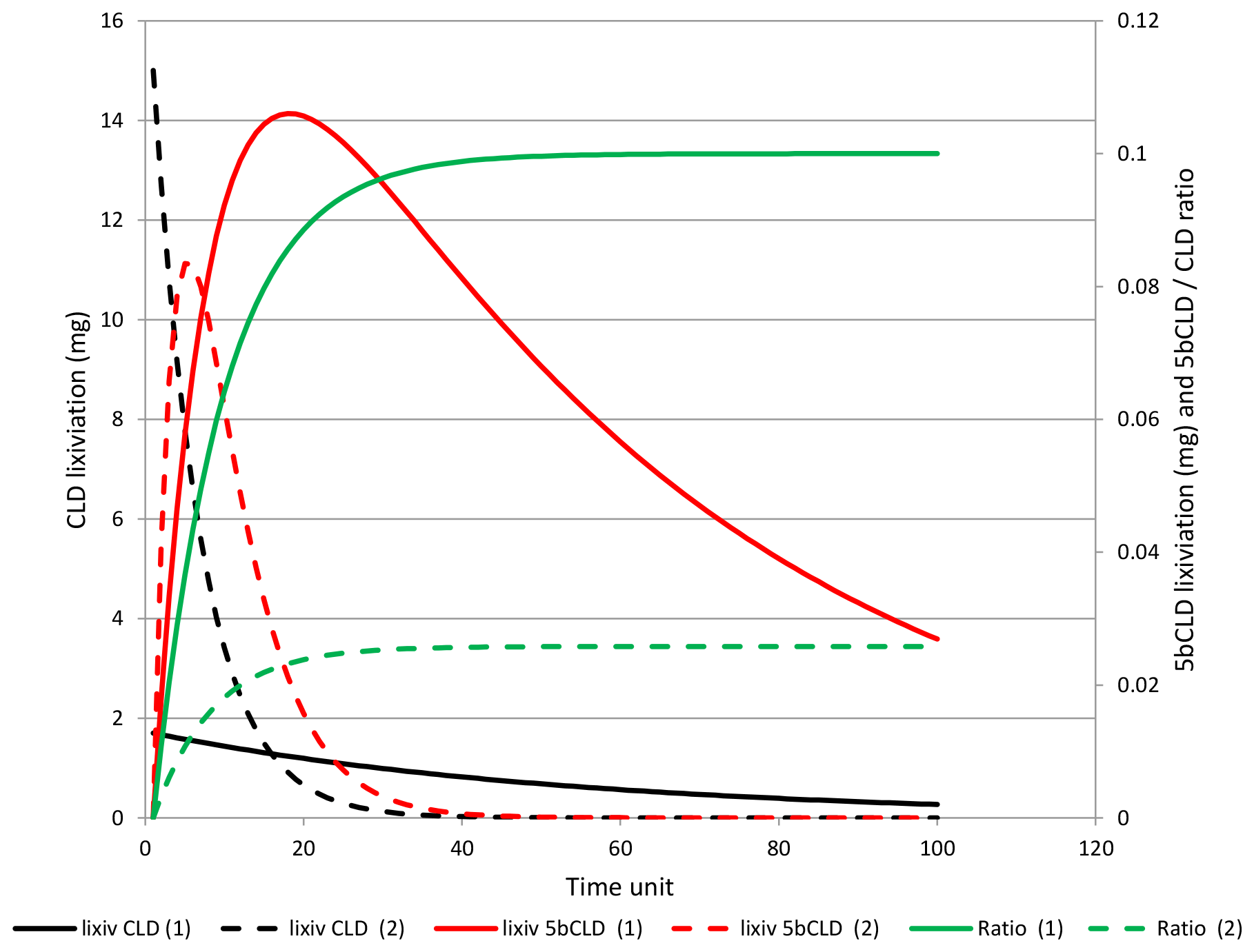
Figure 8Theoretical evolution of CLD and 5bCLD lixiviation, as well as the 5bCLD∕CLD ratio for the two models illustrating (1) conditions for andosols with high soil retention (model And2 in Table 2 – continuous lines) and (2) conditions for nitisols with low soil retention (model Nit1 in Table 2 – dashed line).
The simulation results showed that the ratio increased with time over the entire period up to a plateau (see Fig. 8). A decrease in the ratio was not simulated, although a global trend was noted for our observed data on the whole. At one sampling point, such a decrease could occur with an increase in lixiviation conditions (not shown), which may have been linked to land use changes. More likely, it could have been an artefact due the difficulty in determining low values near the quantification threshold.
CLD decreased exponentially in the modelling approach. The current decrease mainly observed in SW marched these dynamics (linear decrease in log scale, Fig. 6). Interestingly, we found that the decrease rate for andosols (simulation And2 – Fig. 8) was far lower than for nitisols (simulation Nit1). This matched the andosol situation, where no significant decrease in the river was observed.
5bCLD first increased and then decreased at the same time as CLD. This may explain why we found a 5bCLD∕CLD ratio increase, whereas a 5bCLD decrease was observed. Our simulations also showed that T5bCLD must be higher than TCLD otherwise the ratio increased continuously without a plateau. This result was consistent with Devault et al. (2016) who concluded on higher mobility of 5bCLD compared to CLD, and more generally with the results of Dolfing et al. (2012), who showed that transformation products had higher mobility than CLD. Optimisation processes also gave a higher value for T5bCLD (Table 2), given that high ratios are unlikely when TCLD is high (0.15) since it yields a T5bCLD of 1 (meaning that all 5bCLD is leached).
Lastly, despite difficulties in predicting what would happen for each location, our simulations gave interesting insights for a better understanding of the global dynamics of the 5bCLD∕CLD ratio and explained some of the observations in water.
Our results showed high spatial and temporal variability for water CLD content in SW and GW contamination. By relating water CLD content to its metabolite compound, 5bCLD, we highlighted physical conditions relative to soils and geology that may explain its variability in water, but also in the dynamics of pollution trends. We summarised our conclusions in a conceptual scheme presented below. But first, let us specify the interpretation framework.
4.1 Main assumptions about CLD transfer
In our study, we focused on long-term trends for CLD and 5bCLD concentration in water, along with their ratio. We considered that the main process determining pollutant concentrations in water was relative to CLD desorption by water infiltrating the soil. We assumed this hypothesis for different reasons.
Firstly, rain water mainly infiltrates the soil. In fact, given the high soil infiltration rate (saturated hydraulic conductivity over 60 mm h−1; Cattan et al., 2006; Crabit et al., 2016), most rainfall infiltrates the soil (about 95 % on a plot scale according to Cabidoche et al., 2009; more than 90 % on a watershed scale according to Charlier et al., 2008, 2011), generating either subsurface or deep flows. Consequently, transportation by surface runoff is low. Cabidoche et al. (2009) found that CLD concentration in surface runoff was more than 3 times lower than in drainage, while the runoff volume was 10 times lower than the drainage volume. They consequently discarded loads in surface runoff that amounted to less than 1∕30 of those in drainage on a plot scale.
Secondly, soils have little erodibility: Cabidoche et al. (2009) found that “All the soil types in FWI are acidic, which prevents clay dispersion and sheet erosion. Hydric erosion appears to be due only to bad soil management practices, which concentrate runoff that then forms streams that are able to carry aggregates”. Thus, erosion from cultivated soils is probably not a major method of CLD transportation. Moreover, given the high contribution of erosion from river beds and from non-contaminated areas in the upstream zone (due mostly to torrential type flow of rivers in FWI), the impact of surface water contamination by sediments was considered as a minor process.
Lastly, by neglecting transport via surface runoff (since sampling mainly occurred outside storm event periods), we probably underestimated pollutant exportation. Thus, we expected that it should not have a great impact on the long-term dynamics of concentrations and ratios in rivers, which is one of the main topics of our paper.
4.2 CLD is degraded and contamination decreases
First of all, the CLD content in SW tallied with the areas where CLD had been applied, i.e. in banana cropping areas, irrespective of geology and soils. This was consistent with a global link between the location of contaminated soil areas and the location of contaminated rivers, as shown on a watershed scale by Della Rossa (2017). Surprisingly, we found that, overall, the soil type had no significant effect on water CLD content in SW, although large differences in CLD content were usually encountered in soils (Clostre et al., 2015; Devault et al., 2016). This paradoxical result was consistent with previous work showing that the most contaminated soils are not the most contaminant for water, owing to their different capacity to retain the molecule (Cabidoche et al., 2009; Levillain et al., 2012; Woignier et al., 2012). In other words, two types of soils with different CLD contents may release the same quantity of CLD into water. However, our simulations showed (see Fig. 8) that over a long timescale, CLD contents in a river will quickly decrease for basins draining soils such as nitisols, due to their low capacity to retain CLD.
In this environment, our results were in line with CLD degradation, being visible over a decadal time period despite its strong persistence in the environment. This was hypothesised by observing the distribution of 5bCLD∕CLD ratios in water (median of 0.03; first centile of 0.006) with a far higher median and first centile value than in the commercial products Kepone® and Curlone® used in FWI (mean ratio of 0.00077±0.00027; Devault et al., 2016). This was consistent with the result obtained by Devault et al. (2016), who found high 5bCLD∕CLD ratios in soils and, in particular, larger amounts of 5bCLD than should have been applied using commercial formulations.
The water CLD content in SW decreased as well as the water 5bCLD content and the 5bCLD∕CLD ratio. Given the mean Sen trends of about −0.008 for CLD (see Sect. 3.3.2), it takes about 40 years to yield the threshold of 0.1 µg L−1 during baseflow periods (flood flow periods being rarely sampled) given a current concentration of 0.5 µg L−1 on average. This trend was higher than that expected by Cabidoche et al. (2009), maybe because the authors underestimated the degradation process, which is still not greatly documented. However, it was consistent with the results obtained by Crabit (2016) based on a storage approach that assessed the duration of CLD pollution of a river of a watershed at 60 years. These results on the island of Martinique could indeed be extrapolated to other CLD-contaminated areas, such as in the Guadeloupe archipelago (FWI) where CLD was also intensively applied in banana plantations.
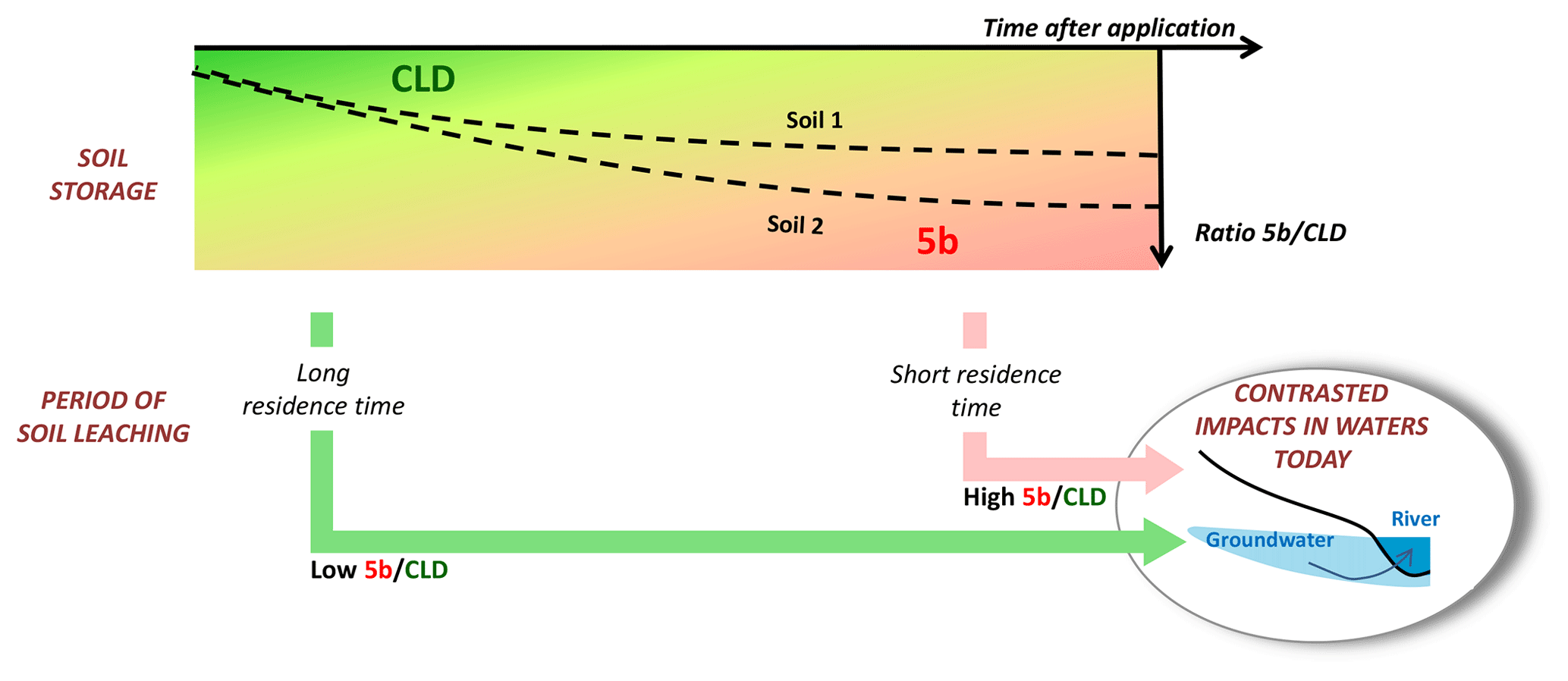
Figure 9CLD fate in soils and residence time combined to explain 5bCLD∕CLD ratio levels in SW. For SW draining GW with a long residence time, leaching occurred during the application period with a low 5bCLD∕CLD ratio whatever the soil type. For SW water draining GW with a short residence time, leaching occurs nowadays from soil with a higher 5bCLD∕CLD ratio depending on soils and reflecting CLD fate in soils.
4.3 Hypothesis relative to leaching processes
One of the main questions in this paper was what the 5bCLD∕CLD ratio represents. To answer this sensitive issue, we differentiated between three dimensions: a temporal dimension, because the 5bCLD∕CLD ratio is assumed to increase over time as degradation progresses; a spatial dimension, since the 5bCLD∕CLD ratio may depend on local degradation conditions; a dynamic dimension, since the 5bCLD∕CLD ratio may depend on the mobility properties of both molecules, CLD and 5bCLD.
The temporal dimension was firstly related to the long application period (from 1970 to 1993 for CLD), given that land-use changes led to different application phases in the 70s and 80s and that land-use changes are correlated with soil contamination levels (Desprats et al., 2004). Secondly, comparing simulation results to measurement time series, the temporal dimension could also be grasped by observing GW, if we consider that the residence time within the aquifer gives a temporal window on the water infiltration conditions (Gourcy et al., 2009; Tesoriero et al., 2007). The residence time – estimated by the water apparent age – depends on hydrogeological properties, and thus to the geological context (type of lithology and its weathering level, geometry of the geological deposits, etc.). For example, we observed that high 5bCLD∕CLD ratios were mainly located in the waters of northern Martinique, where rivers drain recent geological formations. In that area, unweathered formations favour rapid transfers and thus low GW residence times of several years (Arnaud et al., 2017; Gourcy et al., 2009). Thus, in that area, GW is young and probably today mainly composed of waters that percolated in the last decade with a 5bCLD∕CLD ratio close to the current 5bCLD∕CLD ratio in soil leaching waters. Conversely, the higher groundwater residence times in more weathered geological formations probably characterise older GW (residence time of several decades) where the 5bCLD∕CLD ratio may reflect an earlier 5bCLD∕CLD ratio in soil leaching waters – closer to the ratio in the commercial product – during periods of application or just several years after, leading to lower 5bCLD∕CLD ratios in water.
The spatial dimension is hard to grasp since some of the variability can be attributed to the spatio-temporal variability of land-use changes over the application period. Considering that soil might be an important factor, the results from Clostre et al. (2015) show that the distribution of the 5bCLD∕CLD ratio differs little from one soil to another, with a median value of around 0.011 [0.002, 0.077] in andosols and 0.017 [0.007, 0.081] in nitisols. This does not mean that degradation does not depend on soil, but it does mean that we cannot assess the effect of soil on degradation. It is interesting to note that the simulations accounting for nitisols and andosols in Table 2 give close values of 0.14 % and 0.16 % for the degradation rate, respectively. The soil factor could therefore not be considered decisive in explaining spatial degradation intensity.
For the dynamic dimension, our theoretical leaching model helped to represent how contamination evolved. On the whole, the simulations accounting roughly for andosol and nitisol conditions tallied well with our observations or with results from the literature: (i) a large decrease in CLD was associated with a low 5bCLD∕CLD ratio, and (ii) nitisol situations were more conducive to a contamination decrease than andosol situations, considering pollution duration as noted by Cabidoche et al. (2009).
Lastly, this discussion shows that the combined role of geology and soils together may explain 5bCLD∕CLD ratio levels. In a comprehensive way, we derived a conceptual scheme of water contamination on a regional scale.
4.4 A conceptual scheme of water contamination on a regional scale
We propose a conceptual scheme in Fig. 9 to explain differences in 5bCLD∕CLD ratios in water. We first assumed that degradation occurs in soils. This process, which is combined with other processes determining CLD and 5bCLD fate in soil, results in a general increase in water 5bCLD content and in the 5bCLD∕CLD ratio, which is more or less pronounced depending on the soil. Hydrogeology teaches us that SW today could either be a signal of ancient infiltrations and transfers underground, several decades ago, when 5bCLD∕CLD ratios in soils were low (long residence time), or a signal of recent percolations, several years ago, when 5bCLD∕CLD ratios in soils were high (short residence time). Thus, soil properties and residence times both contribute to explaining the current impact on water quality in SW. This explanation is consistent with high 5bCLD∕CLD ratios in northern Martinique on recent geological formations, and low 5bCLD∕CLD ratios elsewhere. For high 5bCLD∕CLD ratios in the south on vertisols, we can speculate that the degradation process was greater in this soil type (like soil 2 in Fig. 9) because lixiviation is lower in the southern area with a lower rainfall rate. This may explain the higher 5bCLD∕CLD ratios in SW, as simulated by a previous model, despite a longer residence time in the aquifers.
All of these results identify a set of conditions that favour the disappearance of CLD from the environment, namely ferralsols with low retention properties on older geological formations, while others – notably andosols with high retention rates on recent formations – are more risky.
The aim of this paper was to identify conditions that are conducive to a decrease in organochlorine pollution levels in Martinique (FWI). We adopted an unusual approach that accounted, on the one hand, for the interactions between aquifers and rivers on a watershed scale and, on the other hand, for the fate of CLD and its compound 5bCLD. This approach was fruitful and led to the proposal of a global scheme of water contamination on a regional scale, accounting for physical conditions relative to soils and geology. This scheme coherently links the various amounts of chlordecone (CLD) and its metabolite 5bCLD in SW and GW. It explains their variability in water, but also in the dynamics of pollution trends.
Our results have several implications for evaluating diffuse pollution of agricultural origin. The spatial analysis of metabolite–parent compounds provided some interesting information for identifying risky areas, or areas where persistent pollutants are more likely decreasing. This also provided some insights into key parameters that control these conditions and environmental vulnerability to agricultural pollution. It led to implications regarding where and how to act to reduce impacts (e.g. choice of crops according to pollution levels, since some plants are less sensitive to contamination than others – see Clostre et al., 2015; constraints on water management, such as drinking water and irrigation; choice of priority areas to test decontamination processes; setting up compensation plans according to the risk). Another implication is to promote continuous long-term observations as opposed to one-off sampling, completing modelling approaches: in our case, long CLD time series revealed a faster decrease than that expected by previous model predictions. Lastly, such a spatial and temporal overview is required on a large scale to help stakeholders manage pollution on a territory scale, accounting for the main characteristics of the landscape. This is the main challenge for the OPA-C Observatory in FWI (Cattan et al., 2017).
The datasets used in this article can be obtained by contacting Philippe Cattan (philippe.cattan@cirad.fr) and Jean-Baptiste Charlier (j.charlier@brgm.fr).
LA and JG were involved in data collection and first interpretation. FC and MJ merged the data, performed the first data analysis and gathered the contributing authors. PL provided statistical processing. PC and JBC were involved in data interpretation, conceptual modelling, and manuscript preparation with contributions from all co-authors.
The authors declare that they have no conflict of interest.
We are grateful to the Water Office, the general council, and the
environment, planning and housing agency in Martinique for the data they
provided on surface waters. Data sets on groundwater were provided by BRGM.
We would like to thank the LDA26 and BRGM laboratories for pesticide
analyses.
Edited by: Marnik
Vanclooster
Reviewed by: Stefan Reichenberger and one
anonymous referee
Adelinet, M., Fortin, J., d'Ozouville, N., and Violette, S.: The relationship between hydrodynamic properties and weathering of soils derived from volcanic rocks, Galapagos Islands (Ecuador), Environ. Geol., 56, 45–58, https://doi.org/10.1007/s00254-007-1138-3, 2008.
AFNOR: Water quality – Protocol for the initial method performance assessment in a laboratory, La Plaine Saint-Denis, France, AFNOR, 2009.
Arias-Estévez, M., López-Periago, E., Martínez-Carballo, E., Simal-Gándara, J., Mejuto, J.-C., and García-Río, L.: The mobility and degradation of pesticides in soils and the pollution of groundwater resources, Agric. Ecosyst. Environ., 123, 247–260, https://doi.org/10.1016/j.agee.2007.07.011, 2008.
Arnaud, L., Charlier, J.-B., Ducreux, L., and Taïlamé, A.-L.: Groundwater quality assessment, Crisis Management of Chronic Pollution: Contaminated Soil and Human Health, CRC Press, Boca Raton, Florida, USA, 2017.
Bexfield, L. M.: Decadal-Scale Changes of Pesticides in Ground Water of the United States, 1993–2003, J. Environ. Qual., 37, Supplement S-226–S-239, https://doi.org/10.2134/jeq2007.0054, 2008.
Bocquene, G. and Franco, A.: Pesticide contamination of the coastline of Martinique, Mar. Pollut. Bull., 51, 612–619, 2005.
Borsetti, A. P. and Roach, J. A. G.: Identification of kepone alteration products in soil and mullet, Bull. Environ. Contam. Toxicol., 20, 241–247, 1978.
Brunet, D., Woignier, T., Lesueur-Jannoyer, M., Achard, R., Rangon, L., and Barthès, B. G.: Determination of soil content in chlordecone (organochlorine pesticide) using near infrared reflectance spectroscopy (NIRS), Environ. Pollut., 157, 3120–3125, https://doi.org/10.1016/j.envpol.2009.05.026, 2009.
Cabidoche, Y.-M., Achard, R., Cattan, P., Clermont-Dauphin, C., Massat, F., and Sansoulet, J.: Long-term pollution by chlordecone of tropical volcanic soils in the French West Indies: A simple leaching model accounts for current residue, Environ. Pollut. Spec. Issue Sect. Ozone Mediterr. Ecol. Plants People Probl., 157, 1697–1705, 2009.
Cannon, S. B., Veazey, J. M., Jackson, R. S., Burse, V. W., Hayes, C., Straub, W. E., Landrigan, P. J., and Liddle, J. A.: Epidemic kepone poisoning in chemical workers, Am. J. Epidemiol., 107, 529–537, 1978.
Cattan, P., Cabidoche, Y.-M., Lacas, J.-G., and Voltz, M.: Effects of Tillage and mulching on runoff under banana (Musa spp.) on a tropical Andosol, Soil Tillage Res., 86, 38–51, 2006.
Cattan, P., Tonneau, J. P., Charlier, J.-B., Ducreux, L., Voltz, M., Bricquet, J.-P., Andrieux, P., Arnaud, L., and Jannoyer, M.: The challenge of knowledge representation to better understand environmental pollution, in Crisis Management of Chronic Pollution: Contaminated Soil and Human Health, CRC Press, Boca Raton, Florida, USA, 2017.
Charlier, J.-B., Cattan, P., Moussa, R., and Voltz, M.: Hydrological behaviour and modelling of a volcanic tropical cultivated catchment, Hydrol. Process., 22, 4355–4370, 2008.
Charlier, J.-B., Cattan, P., Voltz, M., and Moussa, R.: Transport of a Nematicide in Surface and Groundwaters in a Tropical Volcanic Catchment, J. Environ. Qual., 38, 1031–1041, https://doi.org/10.2134/jeq2008.0355, 2009.
Charlier, J.-B., Lachassagne, P., Ladouche, B., Cattan, P., Moussa, R., and Voltz, M.: Structure and hydrogeological functioning of an insular tropical humid andesitic volcanic watershed: A multi-disciplinary experimental approach, J. Hydrol., 398, 155–170, https://doi.org/10.1016/j.jhydrol.2010.10.006, 2011.
Charlier, J.-B., Arnaud, L., Ducreux, L., Ladouche, B., Dewandel, B., Plet, J., Lesueur-Jannoyer, M., and Cattan, P.: Caractérisation de la contamination par la chlordécone des eaux et des sols des bassins versants pilotes guadeloupéen et martiniquais, rapport du projet CHLOR-EAU-SOL, ONEMA, BRGM, CIRAD, Petit-Bourg, Guadeloupe, 2015.
Clostre, F., Cattan, P., Gaude, J.-M., Carles, C., Letourmy, P., and Lesueur-Jannoyer, M.: Comparative fate of an organochlorine, chlordecone, and a related compound, chlordecone-5b-hydro, in soils and plants, Sci. Total Environ., 532, 292–300, https://doi.org/10.1016/j.scitotenv.2015.06.026, 2015.
Coat, S., Monti, D., Legendre, P., Bouchon, C., Massat, F., and Lepoint, G.: Organochlorine pollution in tropical rivers (Guadeloupe): Role of ecological factors in food web bioaccumulation, Environ. Pollut., 159, 1692–1701, https://doi.org/10.1016/j.envpol.2011.02.036, 2011.
Colmet-Daage, F., Lagache, P., de Crécy, J., Gautheyrou, J., Gautheyrou, M., and de Lannoy, M.: Caractéristiques de quelques groupes de sols dérivés de roches volcaniques aux Antilles françaises, Cah. ORSTOMSérie Pédologie III, 3, 91–121, 1965.
Cordier, S., Muckle, G., Kadhel, P., Rouget, F., Costet, N., Dallaire, R., Boucher, O., and Multigner, L.: Chlordecone Impact on Pregnancy and Child Development in French West Indies, Crisis Management of Chronic Pollution: Contaminated Soil and Human Health, CRC Press, Boca Raton, Florida, USA, 2017.
Crabit, A., Cattan, P., Colin, F., and Voltz, M.: Soil and river contamination patterns of chlordecone in a tropical volcanic catchment in the French West Indies (Guadeloupe), Environ. Pollut., 212, 615–626, https://doi.org/10.1016/j.envpol.2016.02.055, 2016.
Della Rossa, P., Jannoyer, M., Mottes, C., Plet, J., Bazizi, A., Arnaud, L., Jestin, A., Woignier, T., Gaude, J.-M., and Cattan, P.: Linking current river pollution to historical pesticide use: Insights for territorial management?, Sci. Total Environ., 574, 1232–1242, https://doi.org/10.1016/j.scitotenv.2016.07.065, 2017.
Desprats, J.-F., Comte, J.-P., and Chabrier, C.: Cartographie du risque de pollution des sols de Martinique par les organochlorés, BRGM/RP-53262-FR report, Fort de France, Martinique, 23 pp., 2004.
Devault, D. A., Laplanche, C., Pascaline, H., Bristeau, S., Mouvet, C., and Macarie, H.: Natural transformation of chlordecone into 5b-hydrochlordecone in French West Indies soils: statistical evidence for investigating long-term persistence of organic pollutants, Environ. Sci. Pollut. Res., 23, 81–97, https://doi.org/10.1007/s11356-015-4865-0, 2016.
Dolfing, J., Novak, I., Archelas, A., and Macarie, H.: Gibbs Free Energy of Formation of Chlordecone and Potential Degradation Products: Implications for Remediation Strategies and Environmental Fate, Environ. Sci. Technol., 46, 8131–8139, https://doi.org/10.1021/es301165p, 2012.
European Union: Council Directive 98/83/EC of 3 November 1998 on the quality of water intended for human consumption, Brussels, 1998.
European Union: Directive 2000/60/EC of the European Parliament and of the Council of 23 October 2000 establishing a framework for Community action in the field of water policy, Luxembourg, 2000.
Farlin, J., Bayerle, M., Pittois, D., and Gallé, T.: Estimating Pesticide Attenuation From Water Dating and the Ratio of Metabolite to Parent Compound, Groundwater, 55, 550–557, https://doi.org/10.1111/gwat.12499, 2017.
Fernández-Bayo, J. D., Saison, C., Voltz, M., Disko, U., Hofmann, D., and Berns, A. E.: Chlordecone fate and mineralisation in a tropical soil (andosol) microcosm under aerobic conditions, Sci. Total Environ., 463–464, 395–403, https://doi.org/10.1016/j.scitotenv.2013.06.044, 2013.
French government: Décret no. 2001–1220 du 20 décembre 2001 relatif aux eaux destinées à la consommation humaine, à l'exclusion des eaux minérales naturelles, 2001.
Gassmann, M., Stamm, C., Olsson, O., Lange, J., Kümmerer, K., and Weiler, M.: Model-based estimation of pesticides and transformation products and their export pathways in a headwater catchment, Hydrol. Earth Syst. Sci., 17, 5213–5228, https://doi.org/10.5194/hess-17-5213-2013, 2013.
Germa, A., Quidelleur, X., Labanieh, S., Lahitte, P., and Chauvel, C.: The eruptive history of Morne Jacob volcano (Martinique Island, French West Indies): Geochronology, geomorphology and geochemistry of the earliest volcanism in the recent Lesser Antilles arc, J. Volcanol. Geotherm. Res., 198, 297–310, https://doi.org/10.1016/j.jvolgeores.2010.09.013, 2010.
Germa, A., Quidelleur, X., Labanieh, S., Chauvel, C., and Lahitte, P.: The volcanic evolution of Martinique Island: Insights from K–Ar dating into the Lesser Antilles arc migration since the Oligocene, J. Volcanol. Geotherm. Res., 208, 122–135, https://doi.org/10.1016/j.jvolgeores.2011.09.007, 2011.
Gilbert, R. O.: Statistical methods for environmental pollution monitoring, Wiley, New York, 1987.
Gonzalez, M., Miglioranza, K. B., Shimabukuro, V., Quiroz Londoño, O., Martinez, D., Aizpún, J., and Moreno, V.: Surface and groundwater pollution by organochlorine compounds in a typical soybean system from the south Pampa, Argentina, Environ. Earth Sci., 65, 481–491, https://doi.org/10.1007/s12665-011-1328-x, 2012.
Gourcy, L., Baran, N., and Vittecoq, B.: Improving the knowledge of pesticide and nitrate transfer processes using age-dating tools (CFC, SF6, 3H) in a volcanic island (Martinique, French West Indies), J. Contam. Hydrol., 108, 107–117, https://doi.org/10.1016/j.jconhyd.2009.06.004, 2009.
IUSS Working Group WRB: World reference base for soil resources 2014 – International soil classification system for naming soils and creating legends for soil maps, FAO, Rome, 2014.
Kolpin, D. W., Schnoebelen, D. J., and Thurman, E. M.: Degradates provide insight to spatial and temporal trends of herbicides in ground water, Ground Water, 42, 601–608, 2004.
Lachassagne, P., Aunay, B., Frissant, N., Guilbert, M., and Malard, A.: High-resolution conceptual hydrogeological model of complex basaltic volcanic islands: a Mayotte, Comoros, case study, Terra Nova, 26, 307–321, https://doi.org/10.1111/ter.12102, 2014.
Lapworth, D. J., Gooddy, D. C., Stuart, M. E., Chilton, P. J., Cachandt, G., Knapp, M., and Bishop, S.: Pesticides in groundwater: some observations on temporal and spatial trends, Water Environ. J., 20, 55–64, https://doi.org/10.1111/j.1747-6593.2005.00007.x, 2006.
Lesueur Jannoyer, M., Cattan, P., Woignier, T., and Clostre, F. (Eds.): Crisis management of chronic pollution: contaminated soil and human health, CRC Press, Boca Raton, 2017.
Levillain, J., Cattan, P., Colin, F., Voltz, M., and Cabidoche, Y.-M.: Analysis of environmental and farming factors of soil contamination by a persistent organic pollutant, chlordecone, in a banana production area of French West Indies, Agric. Ecosyst. Environ., 159, 123–132, https://doi.org/10.1016/j.agee.2012.07.005, 2012.
Luellen, D. R., Vadas, G. G., and Unger, M. A.: Kepone in James River fish: 1976–2002, Sci. Total Environ., 358, 286–297, https://doi.org/10.1016/j.scitotenv.2005.08.046, 2006.
Małoszewski, P. and Zuber, A.: Determining the turnover time of groundwater systems with the aid of environmental tracers, J. Hydrol., 57, 207–231, https://doi.org/10.1016/0022-1694(82)90147-0, 1982.
Masih, A., Lal, J. K., and Patel, D.: Contamination and Exposure Profiles of Persistent Organic Pollutants (PAHs and OCPs) in Groundwater at a Terai Belt of North India, Water Qual. Expo. Health, 6, 187–198, https://doi.org/10.1007/s12403-014-0126-6, 2014.
Montuori, P., Cirillo, T., Fasano, E., Nardone, A., Esposito, F., and Triassi, M.: Spatial distribution and partitioning of polychlorinated biphenyl and organochlorine pesticide in water and sediment from Sarno River and Estuary, Southern Italy, Env. Sci. Pollut. Res., 21, 5023–5035, https://doi.org/10.1007/s11356-013-2419-x, 2014.
Morgenstern, U., Daughney, C. J., Leonard, G., Gordon, D., Donath, F. M., and Reeves, R.: Using groundwater age and hydrochemistry to understand sources and dynamics of nutrient contamination through the catchment into Lake Rotorua, New Zealand, Hydrol. Earth Syst. Sci., 19, 803–822, https://doi.org/10.5194/hess-19-803-2015, 2015.
Mottes, C., Lesueur-Jannoyer, M., Charlier, J.-B., Carles, C., Guéné, M., Le Bail, M., and Malézieux, E.: Hydrological and pesticide transfer modeling in a tropical volcanic watershed with the WATPPASS model, J. Hydrol., 529, 909–927, https://doi.org/10.1016/j.jhydrol.2015.09.007, 2015.
Mouvet, C., Dictor, M.-C., Bristeau, S., Breeze, D., and Mercier, A.: Remediation by chemical reduction in laboratory mesocosms of three chlordecone-contaminated tropical soils, Environ. Sci. Pollut. Res., 24, 25500–25512, https://doi.org/10.1007/s11356-016-7582-4, 2017.
Multigner, L., Kadhel, P., Rouget, F., Blanchet, P. and Cordier, S.: Chlordecone exposure and adverse effects in French West Indies populations, Environ. Sci. Pollut. R., 23, 3–8, https://doi.org/10.1007/s11356-015-4621-5, 2016.
Observatoire de l'Eau de la Martinique, Office de L'Eau de la Martinique and Asconit Consultants: Détermination de la contamination des milieux aquatiques par le chlordécone – VOLET 4?: Investigations complémentaires – Renforcement du maillage géographique sur les cours d'eau d'intérêt piscicole, 2012.
Orndorff, S. A. and Colwell, R. R.: Microbial transformation of Kepone, Appl. Environ. Microbiol., 39, 398–406, 1980.
Quantin, P., Balesdent, J., Bouleau, A., Delaune, M., and Feller, C.: Premiers stades d'altération de ponces volcaniques en climat tropical humide (montagne pelée, martinique), Geoderma, 50, 125–148, https://doi.org/10.1016/0016-7061(91)90030-w, 1991.
Ryberg, K. R. and Gilliom, R. J.: Trends in pesticide concentrations and use for major rivers of the United States, Sci. Total Environ., 538, 431–444, https://doi.org/10.1016/j.scitotenv.2015.06.095, 2015.
SAS Institute Inc: SAS/STAT Software: Release 9.3, SAS Institute Inc., Cary, North Carolina, 2002.
Stone, W. W., Gilliom, R. J., and Ryberg, K. R.: Pesticides in U.S. Streams and Rivers: Occurrence and Trends during 1992–2011, Environ. Sci. Technol., 48, 11025–11030, https://doi.org/10.1021/es5025367, 2014.
Tesoriero, A. J., Saad, D. A., Burow, K. R., Frick, E. A., Puckett, L. J., and Barbash, J. E.: Linking ground-water age and chemistry data along flow paths: Implications for trends and transformations of nitrate and pesticides, J. Contam. Hydrol., 94, 139–155, https://doi.org/10.1016/j.jconhyd.2007.05.007, 2007.
UNEP: Report of the Persistent Organic Pollutants Review Committee on the work of its third meeting, Addendum, Risk management evaluation on chlordecone, Geneva, Switzerland, 2007.
US Environmental Protection Agency: Estimation Programs Interface Suite™ for Microsoft® Windows, Washington, DC, USA, 2012.
Vittecoq, B., Reninger, P. A., Violette, S., Martelet, G., Dewandel, B., and Audru, J. C.: Heterogeneity of hydrodynamic properties and groundwater circulation of a coastal andesitic volcanic aquifer controlled by tectonic induced faults and rock fracturing – Martinique island (Lesser Antilles – FWI), J. Hydrol., 529, 1041–1059, https://doi.org/10.1016/j.jhydrol.2015.09.022, 2015.
Wilson, N. K. and Zehr, R. D.: Structures of some Kepone photoproducts and related chlorinated pentacyclodecanes by carbon-13 and proton nuclear magnetic resonance, J. Org. Chem., 44, 1278–1282, https://doi.org/10.1021/jo01322a020, 1979.
Woignier, T., Clostre, F., Macarie, H., and Jannoyer, M.: Chlordecone retention in the fractal structure of volcanic clay, J. Hazard. Mater., 241–242, 224–230, https://doi.org/10.1016/j.jhazmat.2012.09.034, 2012.
Zhang, Z., Huang, J., Yu, G., and Hong, H.: Occurrence of PAHs, PCBs and organochlorine pesticides in the Tonghui River of Beijing, China, Environ. Pollut., 130, 249–261, https://doi.org/10.1016/j.envpol.2003.12.002, 2004.