Modelling Lake Titicaca's daily and monthly evaporation

Lake Titicaca is a crucial water resource in the central part of the Andean mountain range, and it is one of the lakes most affected by climate warming. Since surface evaporation explains most of the lake's water losses, reliable estimates are paramount to the prediction of global warming impacts on Lake Titicaca and to the region's water resource planning and adaptation to climate change. Evaporation estimates were done in the past at monthly time steps and using the four methods as follows: water balance, heat balance, and the mass transfer and Penman's equations. The obtained annual evaporation values showed significant dispersion. This study used new, daily frequency hydro-meteorological measurements. Evaporation losses were calculated following the mentioned methods using both daily records and their monthly averages to assess the impact of higher temporal resolution data in the evaporation estimates. Changes in the lake heat storage needed for the heat balance method were estimated based on the morning water surface temperature, because convection during nights results in a well-mixed top layer every morning over a constant temperature depth. We found that the most reliable method for determining the annual lake evaporation was the heat balance approach, although the Penman equation allows for an easier implementation based on generally available meteorological parameters. The mean annual lake evaporation was found to be 1700 mm year⁻¹. This value is considered an upper limit of the annual evaporation, since the main study period was abnormally warm. The obtained upper limit lowers by 200 mm year⁻¹, the highest evaporation estimation obtained previously, thus reducing the uncertainty in the actual value. Regarding the evaporation estimates using daily and monthly averages, these resulted in minor differences for all methodologies.

1 Introduction

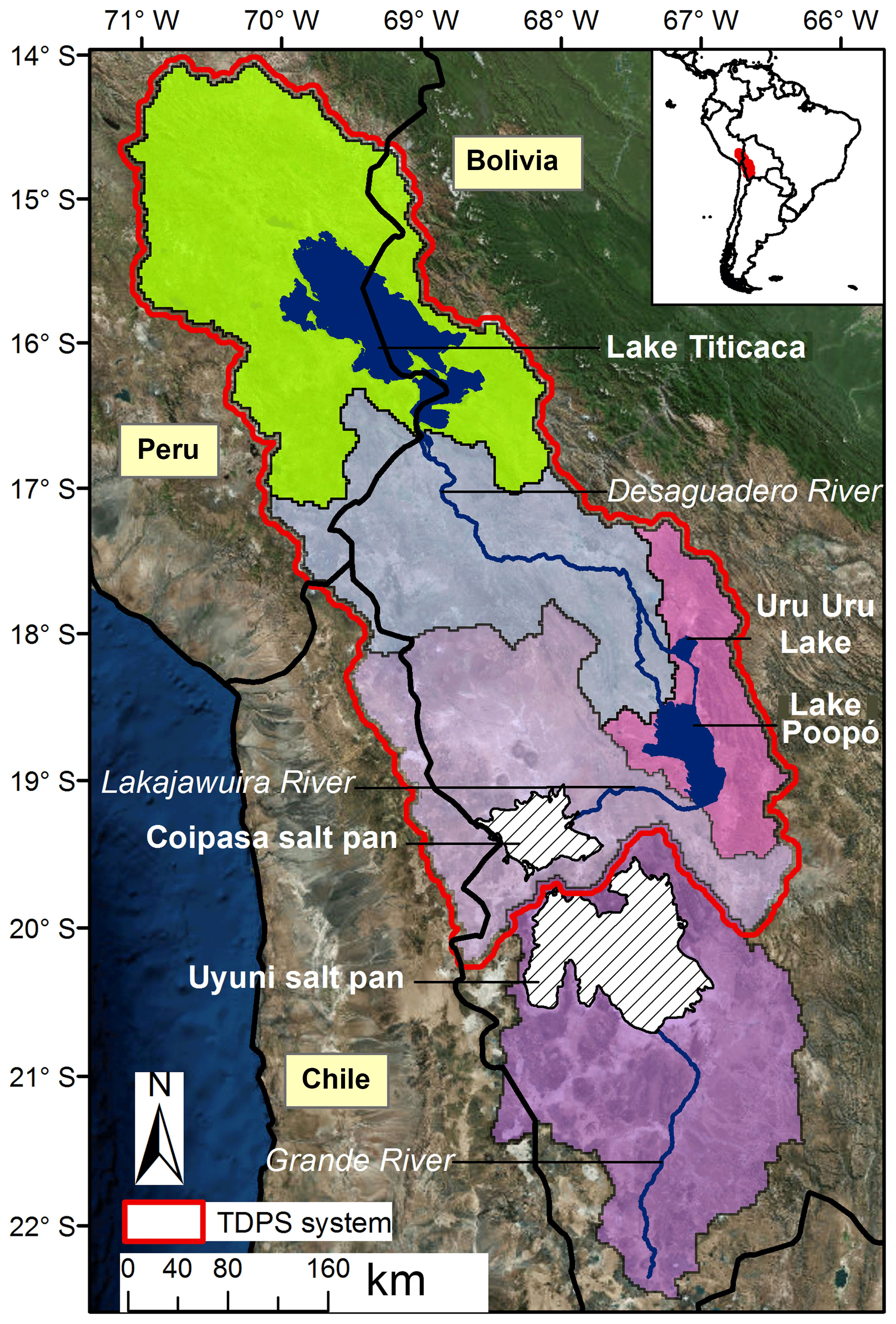
Lake Titicaca, the largest freshwater lake in South America, is located in the endorheic Andean mountain range plateau Altiplano, straddling the border between Peru and Bolivia (Fig. 1). The lake plays an essential role in shaping the semiarid Altiplano climate; feeding the downstream Desaguadero River and Lake Poopó (Pillco and Bengtsson, 2006; Abarca-del-Río et al., 2012); and supplying the inhabitants with water resources for domestic, agricultural, and industrial use (Revollo, 2001). Anthropogenic pressure on the Altiplano water resources has increased during the last decades due to population growth and increased evapotranspiration losses (FAO, 2011; Canedo et al., 2016; Satgé et al., 2017) as well as to industrial pollution (UNEP, 1996; CMLT, 2014). The challenge of managing water resources in the Altiplano Basin is further exacerbated by climate conditions; annual rainfall is highly variable (Garreaud et al., 2003), while warming in this region exceeds the average global trend (López-Moreno et al., 2015), which is expected to intensify the evaporation from the lake surface and the evapotranspiration losses from the whole basin. The combined impact of these pressures becomes evident at the downstream end of the system, where Lake Poopó is situated. In recent years this lake suffered extreme water shortages, including its complete drying out in December 2015 (Satgé et al., 2017).

Figure 1 Lake Titicaca and the TDPS system within the Altiplano.

Lake Titicaca has a large surface area of about 8500 km² on average. Over a certain water surface level, the lake spills out at the south-eastern end and feeds the Desaguadero River. However, the major water output from Lake Titicaca is due to evaporation, which accounts for approximately 90 % of the losses (Roche et al., 1992; Pouyaud, 1993; Talbi et al., 1999; Delclaux et al., 2007). In recent years, Lake Titicaca's level dropped below the outlet threshold for some periods. Thus, a small increase in evaporation or decrease in precipitation may turn the lake into a closed system with no outflow.

Since evaporation dominates the water balance in Lake Titicaca, it is essential to improve the knowledge of the lake's evaporation. This is especially important in light of anthropogenic pressure and due to the evident strong global warming that this region experiences. Previous studies of Lake Titicaca's evaporation have all been based on monthly meteorological observations. Due to the importance of lake evaporation, detailed calculations using daily as well as monthly observations may be necessary. Consequently, this paper investigates different methods for calculating evaporation using both daily and monthly data; in addition we discussed the possibility for the appropriate evaporation models at both timescales to be used on the study the climatic functioning and sensitivity. The main problem with Lake Titicaca's evaporation estimation is the lack of high-resolution temporal data. Taking into account only the mass transfer models for different timescale, Singh and Xu (1997) calculated monthly evaporation. However, doing the same calculations on a daily basis could give radically different results. For both timescales, the evaporation estimation could be more sensitive to vapour pressure. On the other hand, random errors in input data could have a significant effect on evaporation estimation at a monthly scale rather than at a daily scale (Singh et al., 1997).

Lake Titicaca's surface water is cold, with a temperature that remains 12–17 ^∘C throughout the year, and below 40 m depth the temperature is almost constant (Richerson et al., 1977). The water is usually warmer than the air during the daytime, which means that the air immediately above the lake is unstable. The air temperature shows large diurnal variations, often exceeding 15 ^∘C in summer. At an average terrain elevation above 4000 m a.s.l. the solar radiation is strong and the atmospheric pressure is low, which means that the ratio between sensible and latent heat flux (Bowen ratio) is lower than at sea level. To determine the evaporation rate using the aerodynamic mass transfer approach, the atmospheric vapour pressure and surface temperature must be known. Furthermore, a wind function must be used, because the atmosphere over Lake Titicaca is unstable most of the time. This means that the wind function may be different from the function used for most other lakes.

It can generally be assumed that during a year the lake water temperature returns to the value at the beginning of the year. Thus, for the heat balance, it is sufficient to know the annual net radiation, provided that the sensible heat flux can be estimated from the constant Bowen ratio. When using the method for shorter time periods, the time variation of the lake water temperature profile must be known. The heat balance approach and the aerodynamic method can be combined. The Penman method is such a combined approach. A wind function must also be included in this approach.

Previous investigations

One of the first evaporation studies for Lake Titicaca applied the water balance method using measurements for the period 1956–1973 (Carmouze et al., 1977) and estimated a mean annual lake evaporation of 1550 mm year⁻¹. Taylor and Aquize (1984) applied a bulk transfer approach for a shorter period and determined the lake evaporation to be 1350 mm year⁻¹. The largest reported annual evaporation is from using the energy balance approach. Richerson et al. (1977) found the lake evaporation to be equal to 1900 mm year⁻¹. Later, Carmouze (1992) used the same approach and found the lake evaporation to be 1720 mm year⁻¹. Using observations for the period 1965–1983 and the water balance method, Pouyaud et al. (1993) found the mean annual evaporation to be equal to about 1600 mm year⁻¹. Thus, the mean annual evaporation has been estimated in the range 1350–1900 mm year⁻¹. While the precipitation can vary much from year to year, the large range of calculated annual evaporation, 1350 to 1900 mm year⁻¹, is likely to be the result of uncertainties in the evaporation estimations and in the temporal resolution of the measurements. Recently, Delclaux et al. (2007) studied the evaporation from Lake Titicaca using in situ pan-evaporation measurements, energy balance, mass transfer and the Penman methods. They concluded that the mean annual evaporation may be about 1650 mm year⁻¹, with low seasonal variation between 135 mm in July (winter) and 165 mm in November (summer).

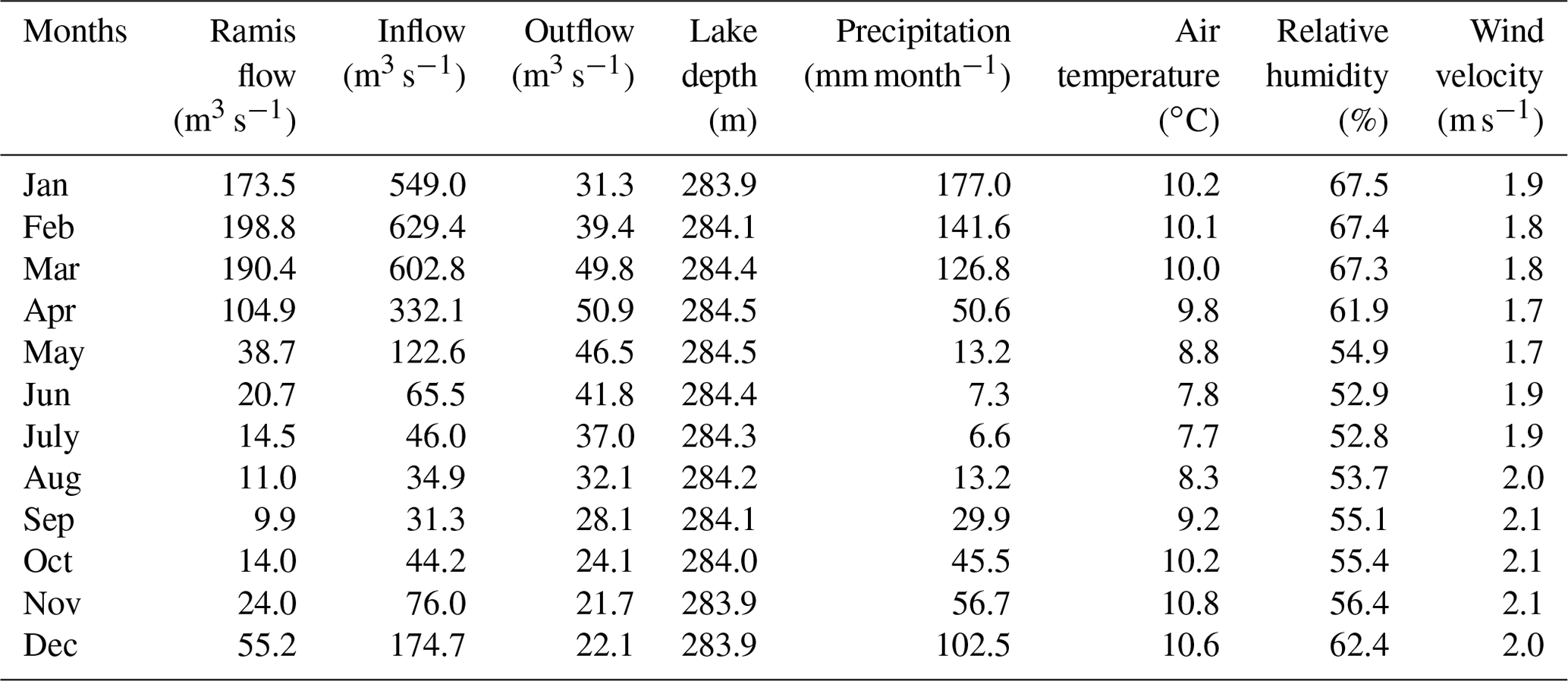
Table 1 Climatological and hydrological components of Lake Titicaca for 1966–2011.

This study applies the methodologies mentioned above using the frequent and accurate hydro-meteorological measurements acquired at Lake Titicaca in 2015 and 2016, with the aim of reducing the uncertainty in evaporation estimates and evaluating the effect of using daily records instead of monthly ones.

2 Study area

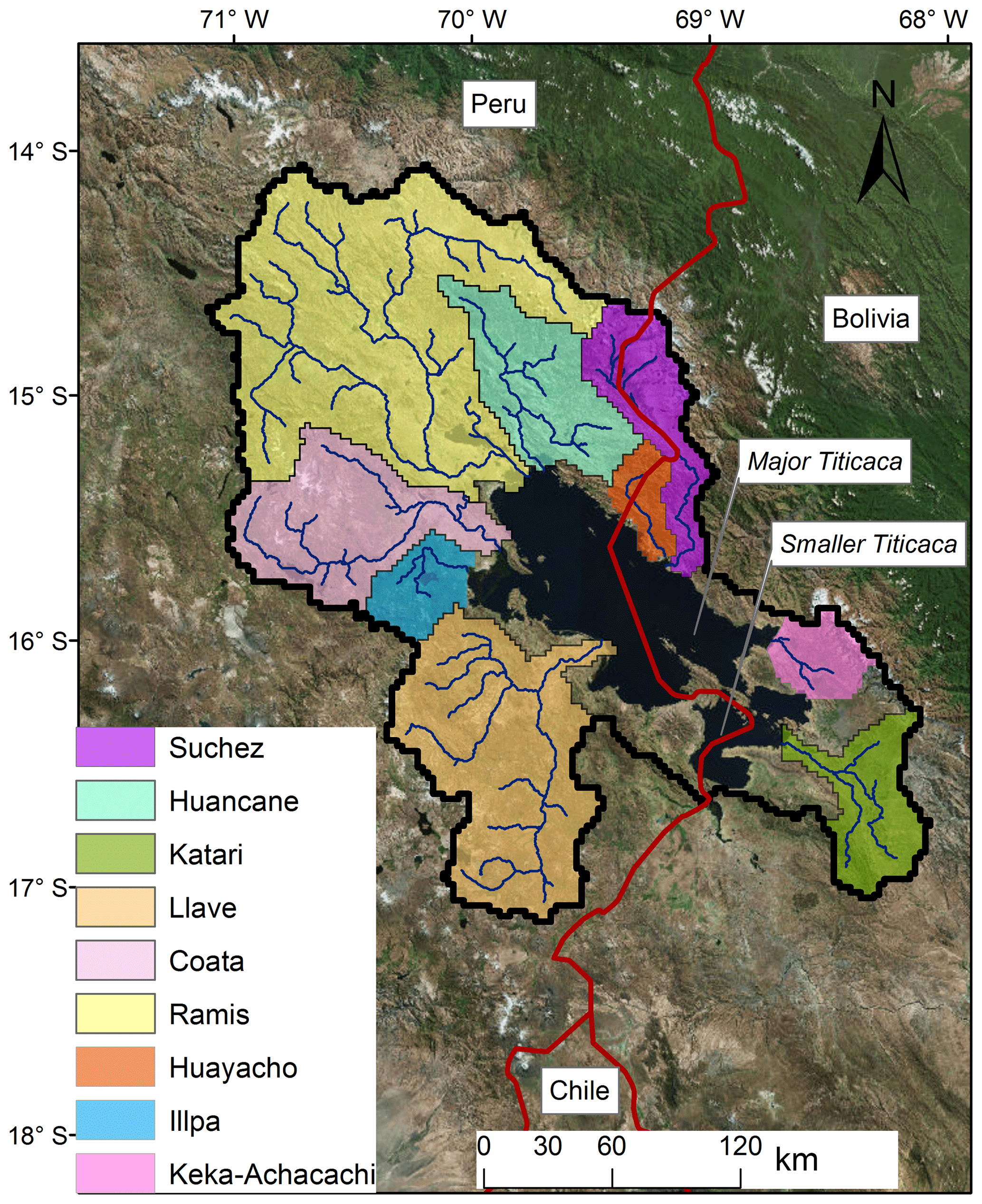
Lake Titicaca is a unique biosphere due to its large depth and volume, high elevation, and tropical latitude. It is located in the northern part of the Peruvian–Bolivian Altiplano, between latitudes of 15^∘45^′ S and 69^∘25^′ W. It is surrounded by the eastern and western Andean Mountains. The total Lake Titicaca basin area, including the lake itself, is close to 57 000 km², with a mean elevation higher than 4000 m a.s.l. The outlet sill is at 3807 m a.s.l. The lake volume is about 903 km³, with a corresponding mean depth of 105 m (Boulange and Aquize, 1981; Wirrmann, 1992). The only outlet is the Desaguadero River, which ends in the shallow Lake Poopó. The modern Lake Titicaca consists of the major Titicaca lake (Lake Chuquito), which is 284 m at the deepest point, and the smaller Titicaca lake (Lake Huiñamarca). The latter lake represents 1200 km², with a maximum depth of 35 m below the spill level. The threshold between the two lake basins is 19 m below the spill level (see Fig. 2). The lake is described by Dejoux and Iltis (1992) and in the Encyclopedia of Lakes and Reservoirs edited by Bengtsson et al. (2012).

Figure 2 Lake Titicaca basin with sub-basins and major and smaller lakes.

2.1 Hydrology

The Lake Titicaca watershed is a part of the TDPS system (Titicaca, Desaguadero, Poopó and Salares) within the Altiplano (Revollo, 2001). Lake Poopó is considered a terminal lake, with only one discharge event into the downstream Coipasa salt pan occurring in the last century (Pillco and Bengtsson, 2006). The basin of Lake Titicaca itself includes the sub-basins Katari, Coata, Huancané, Huaycho, Ilave, Illpa, Keka-Achacachi, Ramis and Suchez. The largest is the Ramis River basin, with an area of 15 000 km², representing 30 % of the total basin (Fig. 2). The mean flow of the Ramis River for the period 1965–2011 was 72 m³ s⁻¹. The mean outflow from Lake Titicaca through the Desaguadero River for the same period was 35 m³ s⁻¹. During those 50 years, Lake Titicaca experienced large changes in water level, with a mean close to 3808.1 m a.s.l., which is about 1 m above the outlet threshold (Pillco and Bengtsson, 2006). From its low to high water level, the Lake Titicaca water surface area might change from a minimum of 7000 to a maximum of 9000 km².

2.2 Climate

The northern part of the Altiplano is semiarid, while the southern part, including the biggest salt pans in the world, is arid (TDPS, 1993). The climate is further characterized by a short wet season (December–March) and a long dry season (April–November; Garreaud et al., 2003). The average precipitation over the Lake Titicaca basin is about 800 mm year⁻¹, out of which more than 70 % fall during the wet season (Garreaud et al., 2003). Over the lake, annual precipitation is assumed to vary from 1200 mm year⁻¹ in the central part to 800 mm year⁻¹ along the shores (TDPS, 1993). January is the wettest (about 180 mm month⁻¹) and July the driest (less than 10 mm) month. In the central and southern parts of the Altiplano, the total annual precipitation is about 350 mm (Roche et al., 1992; Pillco and Bengtsson, 2006) and is less than 200 mm over the Salares in the southernmost areas (Satgé et al., 2016). The seasonal variability of precipitation in the basin is related to changes in the upper troposphere circulation. During the Austral summer, an upper-level cyclone is established to the south-east of the central Andes. The Bolivian high brings easterly winds and allows influx of moisture from the central continent over the plateau during periods, intensifying the precipitation (Garreaud, 1999; Vuille et al., 2000).

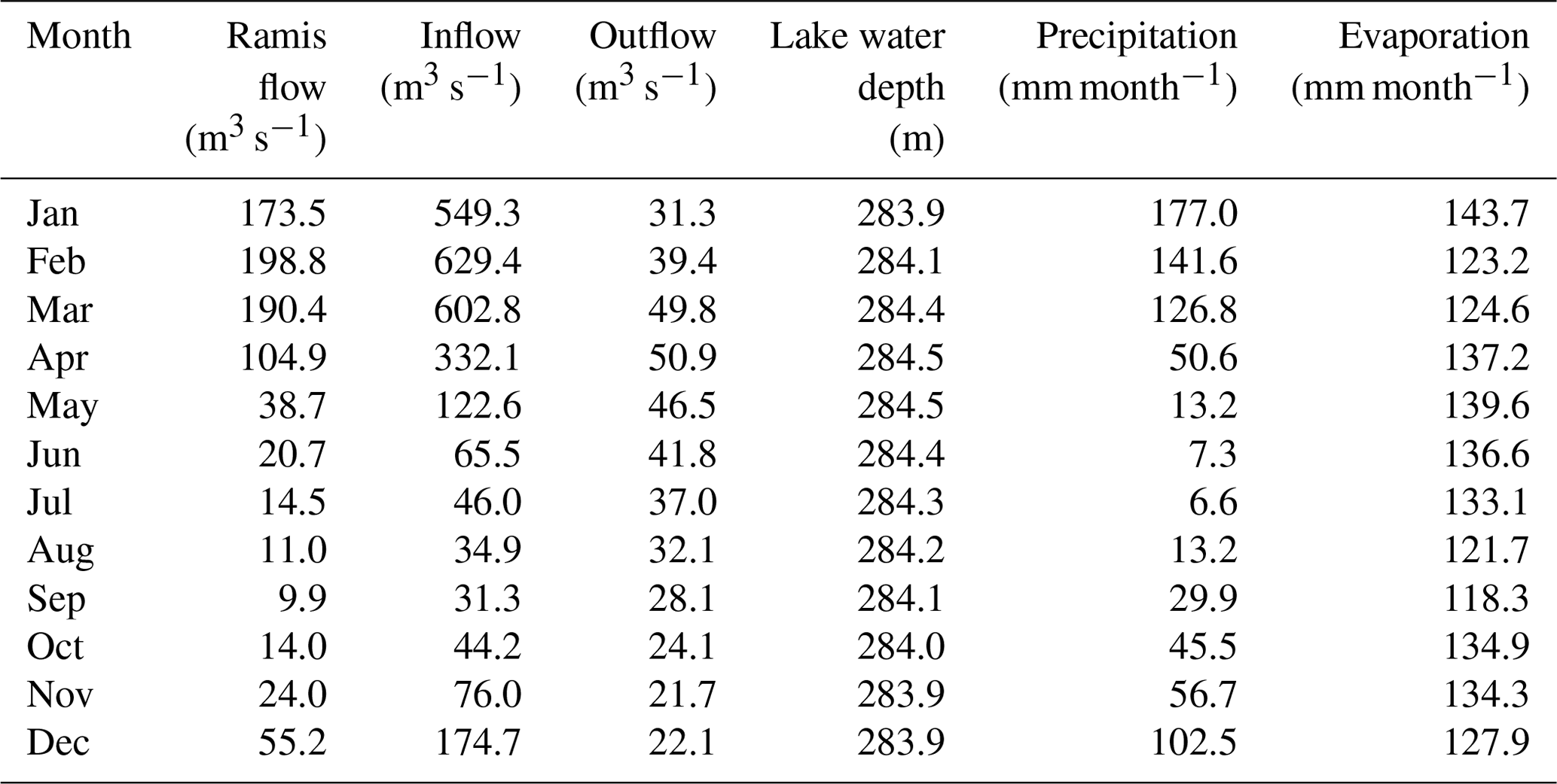
The daily air temperature over Lake Titicaca is rather constant throughout the year, usually varying between 7 and 12 ^∘C but sometimes up to 20 ^∘C in summer. The Titicaca region is more humid than the more southern parts of the Altiplano. The relative humidity varies between 52 % to 68 % as a monthly average, with diurnal variation between 33 % and 80 %. According to Carmouze (1992), the dominant wind on the lake is in the north-west to south-east direction, with mean monthly wind velocity close to 2 m s⁻¹, rarely reaching 5 m s⁻¹ at the daily time step. The general climate and hydrology are summarized in Table 1. The total river inflow was estimated through a representative area approach based on the Ramis River discharge.

3 Methods

Lake evaporation models

Four evaporation estimation conventional methods were applied in this study: water balance, energy balance, mass transfer and the Penman method. These approaches have previously been used by other researchers to estimate Lake Titicaca's evaporation at a monthly time step (Carmouze, 1992; Pouyaud, 1993; Delclaux et al., 2007). The methods are briefly described as follows.

3.1 Energy balance approach

The energy balance approach (Maidment, 1993) which comes from the integral energy balance equation of a reference volume at the air–water interface, the evaporation component in terms of latent heat flux is

$$\begin{array}{}\text{(1)}& {\displaystyle }\mathit{\lambda }E={\displaystyle \frac{R_{\mathrm{n}}-Q_{\mathrm{heat}}}{\mathrm{1}+\mathit{\beta }}},\end{array}$$

where λ is the latent heat vaporization (J kg⁻¹), E is evaporation rate (mm day⁻¹), R_n is net radiation (W m⁻²), Q_heat is heat storage within the water (W m⁻²) and β is the Bowen ratio (Bowen, 1926):

$$\begin{array}{}\text{(2)}& {\displaystyle }& {\displaystyle }\mathit{\beta }=\mathit{\gamma }{\displaystyle \frac{T_{\mathrm{w}}-T_{\mathrm{a}}}{e_{\mathrm{w}}-e_{\mathrm{a}}}},\text{(3)}& {\displaystyle }& {\displaystyle }\mathit{\gamma }={\displaystyle \frac{c_{\mathrm{p}}{p}_{\mathrm{a}}}{\mathrm{0.622}\mathit{\lambda }}},\end{array}$$

where γ is the psychrometric constant (mbar ^∘C⁻¹); T_w and T_a are the surface water and air temperature (^∘C), respectively; e_w and e_a are the water surface and air vapour pressures (Pa), respectively; c_p is the specific heat capacity (J kg^−1 ∘C⁻¹); and Pa is the atmospheric pressure (kg Pa). The psychrometric constant, and thus also the Bowen ratio, are lower at this high altitude than at sea level. The net radiation is the sum of net short-wave and net long-wave radiation. The net short-wave radiation is R_s (1− albedo), where R_s is the solar radiation reaching the lake (W m⁻²). The atmospheric long-wave radiation as well as the back radiation are computed from Stefan's law. The emissivity of the water is well known and was set to 0.98, and the emissivity atmosphere must be known. The emissivity of the atmosphere depends on humidity, temperature and cloudiness. The atmospheric emissivity accounting for clouds was proposed by Crawford and Duchon (1999):

$$\begin{array}{}\text{(4)}& {\displaystyle }& {\displaystyle }{\mathit{\epsilon }}_e=\left(\mathrm{1}-s\right)+s{\mathit{\epsilon }}_o\left(T_{\mathrm{a}},e_{\mathrm{a}}\right),\text{(5)}& {\displaystyle }& {\displaystyle }s={\displaystyle \frac{R_{\mathrm{s}}}{R_{\mathrm{s},o}}},\text{(6)}& {\displaystyle }& {\displaystyle }{R}_{\mathrm{s},o}=R_{\mathrm{a}}{e}^{\left(\frac{-\mathrm{0.0018}{P}_{\mathrm{a}}}{K_{\mathrm{t}}\sin {\mathit{\varphi }}_{\mathrm{24}}}\right)},\text{(7)}& {\displaystyle }& {\displaystyle }{\mathit{\epsilon }}_o=\mathrm{1.18}{\left({\displaystyle \frac{e_{\mathrm{a}}}{T_{\mathrm{a}}}}\right)}^{\frac{\mathrm{1}}{\mathrm{7}}},\end{array}$$

where s is the proxy cloudiness defined as the ratio of measured incoming solar radiation R_s (W m⁻²) to the solar radiation received for the clear-sky conditions R_s,o (W m⁻²), and ε_o is the emissivity in the clear-sky condition, which is determined from the vapour pressure e_a expressed in hPa and T_a temperature in Kelvin. The Φ₂₄ is the mean daily sun angle. The constant 1.18 describes the attenuation defined for the region according to Lhomme et al. (2007). The extraterrestrial solar radiation R_a (W m²) is determined as a function of local latitude and altitude and time of year, using the turbidity coefficient K_t=0.85.

The energy equation is fairly easy to use over a full year, since the lake water usually returns to its initial state when computations were started or when Q_heat equals zero (W m⁻²). When using the approach over shorter periods the variation of the water temperature in the lake must be accounted for. In Eq. (1), the change of heat storage is included. From temperature water profiling observations, it was assumed that the water temperature below 40 m does not change from month to month. The temperature, T_w, above this mixing depth, h_mix (m), changes but remains almost homothermal after convective mixing during the night (Richerson et al., 1977), which also is corroborated by our own field investigations. Thus, the change of heat content can be estimated from measured surface temperature:

$$\begin{array}{}\text{(8)}& {\displaystyle }{Q}_{\mathrm{heat}}=\mathit{\rho }{c}_{\mathrm{p}}{\displaystyle \frac{V_{\mathrm{mix}}}{A_{\mathrm{lake}}}}{\displaystyle \frac{\partial T_{\mathrm{w}}}{\partial t}},\end{array}$$

where ρ is density of water (kg m⁻³), c_p is the specific heat capacity of water and V_mix is the volume above the mixing depth (km⁻³). Carmouze et al. (1992) introduced the concept of the exchange of heat between surface and deep water using the energy balance concept. The results of Carmouze et al. (1992) were compared to the calculation results in the present study.

3.2 Mass transfer approach

The mass transfer aerodynamic approach is used in various models based on Dalton's law (Dalton, 1802). The latent heat transfer is related to the vapour pressure deficit. Most often a linear wind function is used (e.g. Carmouze et al., 1992):

$$\begin{array}{}\text{(9)}& {\displaystyle }E=(a+bU)(e_{\mathrm{w}}-e_{\mathrm{a}}),\end{array}$$

where E is the evaporation rate, U is wind velocity (m s⁻¹) and e_w−e_a is the vapour pressure deficit (mbar). The parameter a accounts for unstable atmospheric conditions. Carmouze et al. (1992) used a=0.17 (mm mbar⁻¹ day⁻¹) and b=0.30 (mm mbar⁻¹ s m⁻¹).

3.3 Penman approach

The Penman equation is a combination of energy balance and mass transfer used for evaluating open water evaporation (Penman, 1948):

$$\begin{array}{}\text{(10)}& {\displaystyle }E={\displaystyle \frac{\mathrm{\Delta }}{\mathrm{\Delta }+\mathit{\gamma }}}{\displaystyle \frac{(R_{\mathrm{n}}-Q_{\mathrm{heat}})}{\mathit{\lambda }\mathit{\rho }}}+{\displaystyle \frac{\mathit{\gamma }}{\mathrm{\Delta }+\mathit{\gamma }}}c(a^{\prime }+b^{\prime }U)(e_{\mathrm{s}}-e_{\mathrm{a}}),\end{array}$$

where E is open water evaporation. The slope of the water pressure–temperature curve is denoted by Δ(K Pa s⁻¹), and e_s−e_a is the saturation deficit of the air (K Pa); here e_a is dependent on the relative humidity (%). Delclaux et al. (2007) applied the Penman equation to Lake Titicaca using $a^{\prime }=\mathrm{0.26}$, $b^{\prime }=\mathrm{0.14}$ and c=1 after optimizing (mm day⁻¹ mbar).

3.4 Lake water balance model

The water balance approach was applied to calculate water levels in Lake Titicaca in a previous study by Pillco and Bengtsson (2007). The water balance is

$$\begin{array}{}\text{(11)}& {\displaystyle }{A}_{\mathrm{lake}}{\displaystyle \frac{\partial h}{\partial t}}=(P-E)A_{\mathrm{lake}}+Q_{\mathrm{in}}-Q_{\mathrm{out}},\end{array}$$

where $\partial h/\partial t$ represents change in water depth; P is precipitation on the lake (mm); E is evaporation from open water (mm day⁻¹); A_lake is water surface of the lake (km⁻²), which is a function of depth; Q_in is inflow to the lake; and Q_out represents the outflow from the lake (m³ s⁻¹). Computations were carried out at a monthly timescale for two periods, one for 1966–2011 and another for 2015–2016. As already pointed out, the most reliable method of computing evaporation over long periods is probably the water balance method. However, the computation only can be general, since the inflow to Lake Titicaca is not measured in all rivers.

3.5 Possible errors when using monthly averages

The evaporation during individual days is not important for the water balance but is only important over longer periods like months. However, since the equations for calculating evaporation are not linear, the monthly evaporation computed from monthly mean meteorological data may differ from what is found when data with a higher time resolution are used. In the aerodynamic approach the wind speed is multiplied by the vapour deficit. The energy balance approach includes the Bowen ratio, which may differ from day to day and can even be negative for certain periods. If high atmospheric vapour pressure is related to strong winds, the aerodynamic equation using monthly means can yield lower evaporation estimates than when daily values are used. This is further discussed below. The Bowen ratio changes during a month. When the net radiation is large, the air temperature is likely to be rather high but is not necessarily related to high vapour pressure. For this situation, the Bowen ratio is relatively high, and the computed evaporation is higher than it would have been using a constant monthly Bowen ratio. This means that when using monthly averages, the computed evaporation will tend to be low.

4 Instrumentation and data

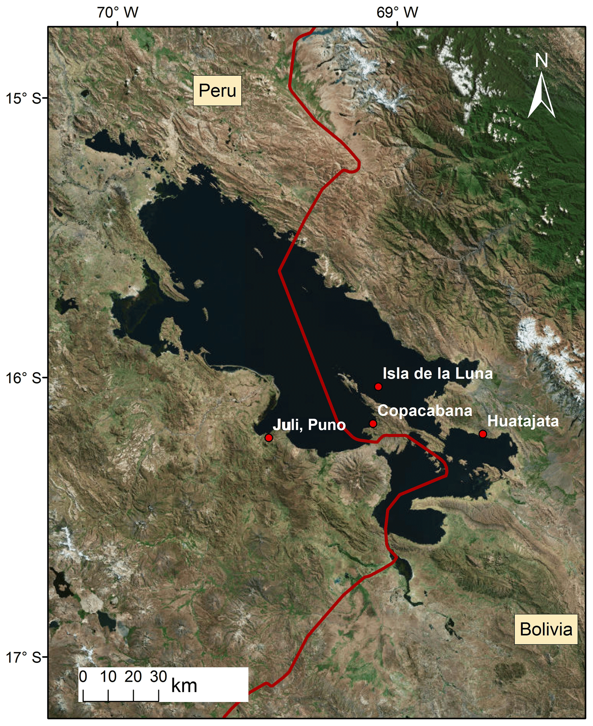
For this study, hydro-meteorological parameters and water surface temperature were measured near Lake Titicaca's bank for 24 consecutive months (2015–2016). Vertical lake temperature profiles were also acquired periodically. Observations were taken at 15 min intervals. These records were averaged to daily and monthly values. A Campbell Scientific research-grade automatic weather station (AWS) was installed at the Isla de la Luna (latitude 16^∘01^′59${}^{\prime \prime }$, longitude 69^∘04^′01${}^{\prime \prime }$), near the shore of Lake Titicaca (Fig. 3). The AWS was equipped with a rain gauge sensor, a CS215 probe for measuring relative humidity and air temperature, an A100R vector anemometer and W200P wind vane to measure wind speed, and a Skye SP1100 pyranometer for solar radiation measurement. The surface water temperature was taken from Juli, Puno (latitude 16^∘12^′58${}^{\prime \prime }$, longitude 69^∘27^′31${}^{\prime \prime }$), at a distance of 42 km from Isla de la Luna. A handheld thermometer was used to measure water surface temperature at 8 h intervals at approximately 60 m from the shoreline. An increased daily surface recorded temperature is representative of heat storage changes.

Hydrological data, such as inflow to the lake, were observed at the outlet of the Ramis River. The outflow through the Desaguadero River was observed at Aguallamaya. This is 40 km downstream of the lake outlet. However, there are only a few tributaries between the lake and this point that may contribute to the data uncertainty. The water level was observed at Huatajata at the daily time step, shown as depth in Table 1. Additional lake water temperature soundings were carried out close to Isla de la Luna (latitude 16^∘30^′00${}^{\prime \prime }$, longitude 69^∘15^′10${}^{\prime \prime }$) for specific days during the summer, spring and winter of the study period, using the Hydrolab DS5 multiparameter data sonde. The sounding reached a maximum lake depth of 95 m, with a water temperature recording for each 5 cm at the surface and each 0.5 m below 1 m depth.

Long-term monthly temperature and wind observations from 1960 onwards were available from the Copacabana weather station mentioned above (Fig. 3; Table 1). The El Alto station observations, 50 km from Copacabana, were used to fill 2.5 % of the missing wind data for the period. The monthly precipitation on the lake was determined using the rain gauge at Copacabana and Puno on the lake shore. The total inflow from all rivers was estimated from a representative area approach assuming the specific run-off to be the same for all rivers entering into Lake Titicaca. The long-term outflow from the lake was measured at the outlet of the lake and treated by Gutiérrez and Molina (2014).

Figure 3 Location of observation points.

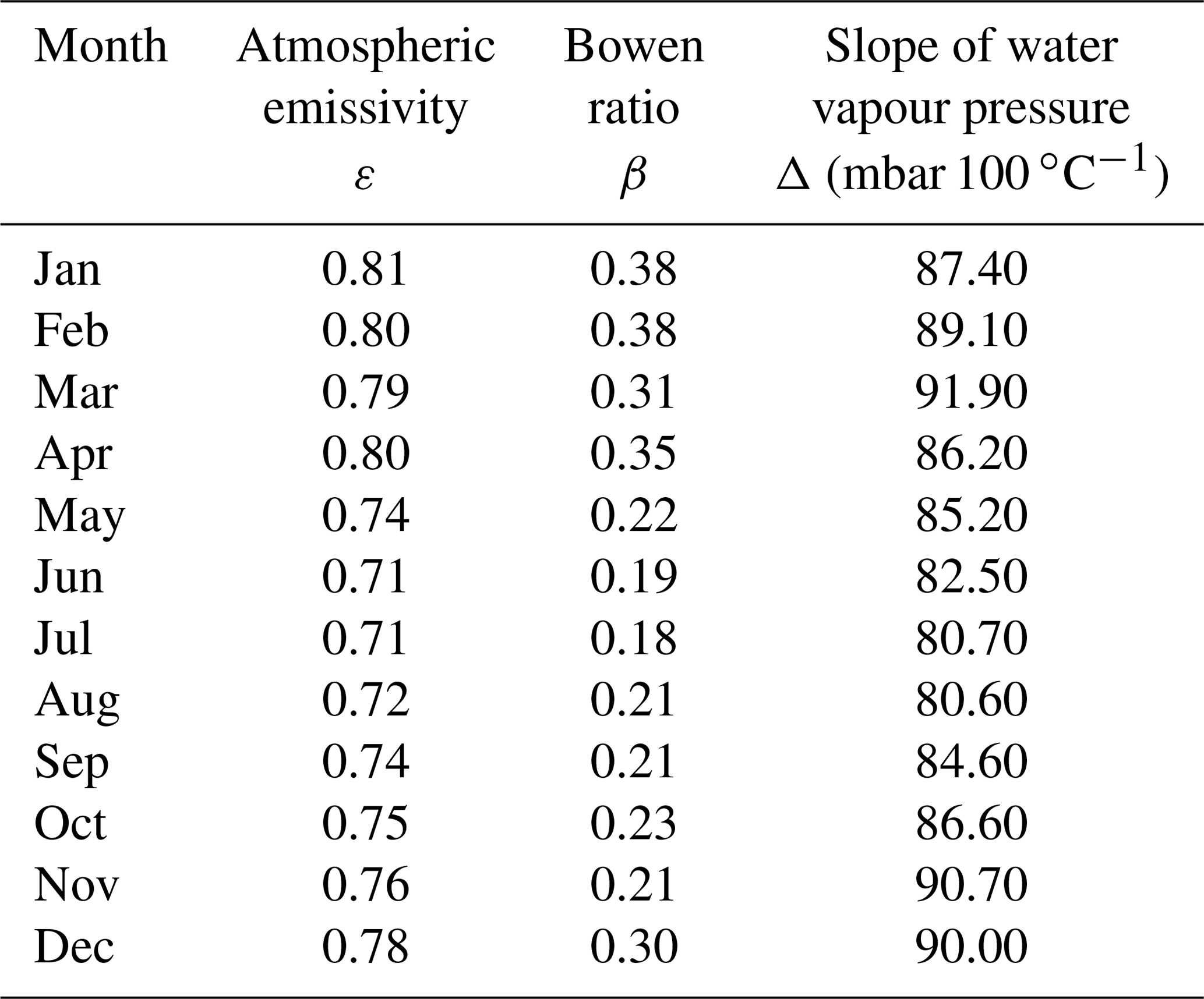
Tables 2 and 3 summarize hydrological and meteorological measurements used in this study. Subscripts for vapour pressure are “w” for water, “s” for saturated air vapour pressure and “a” for actual air vapour pressure. The computed variables required for evaporation calculations are given in Table 4.

Table 2 Monthly mean of hydrological variables observed during the 2015–2016 period.

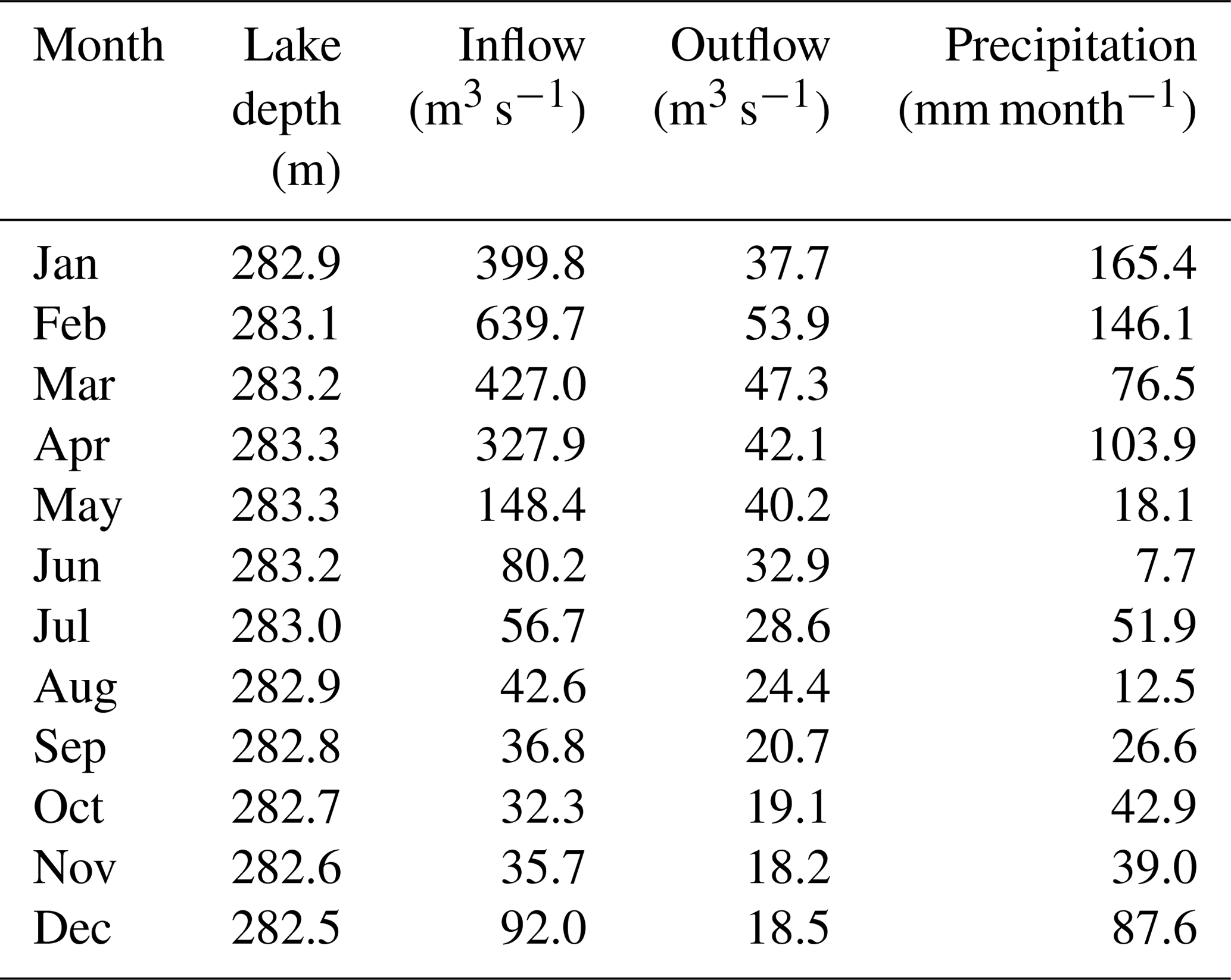
Table 3 Monthly averages of main climatic variables observed during the 2015–2016 period.

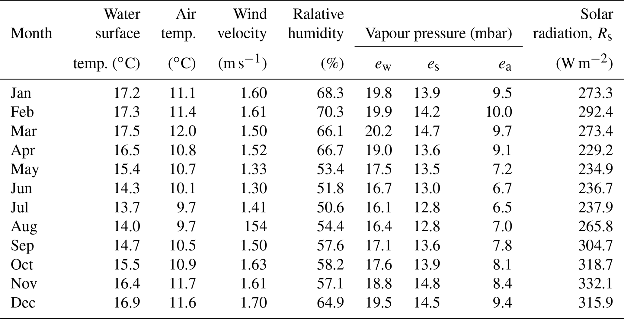
Table 4 Monthly average parameters for evaporation calculations for the 2015–2016 period.

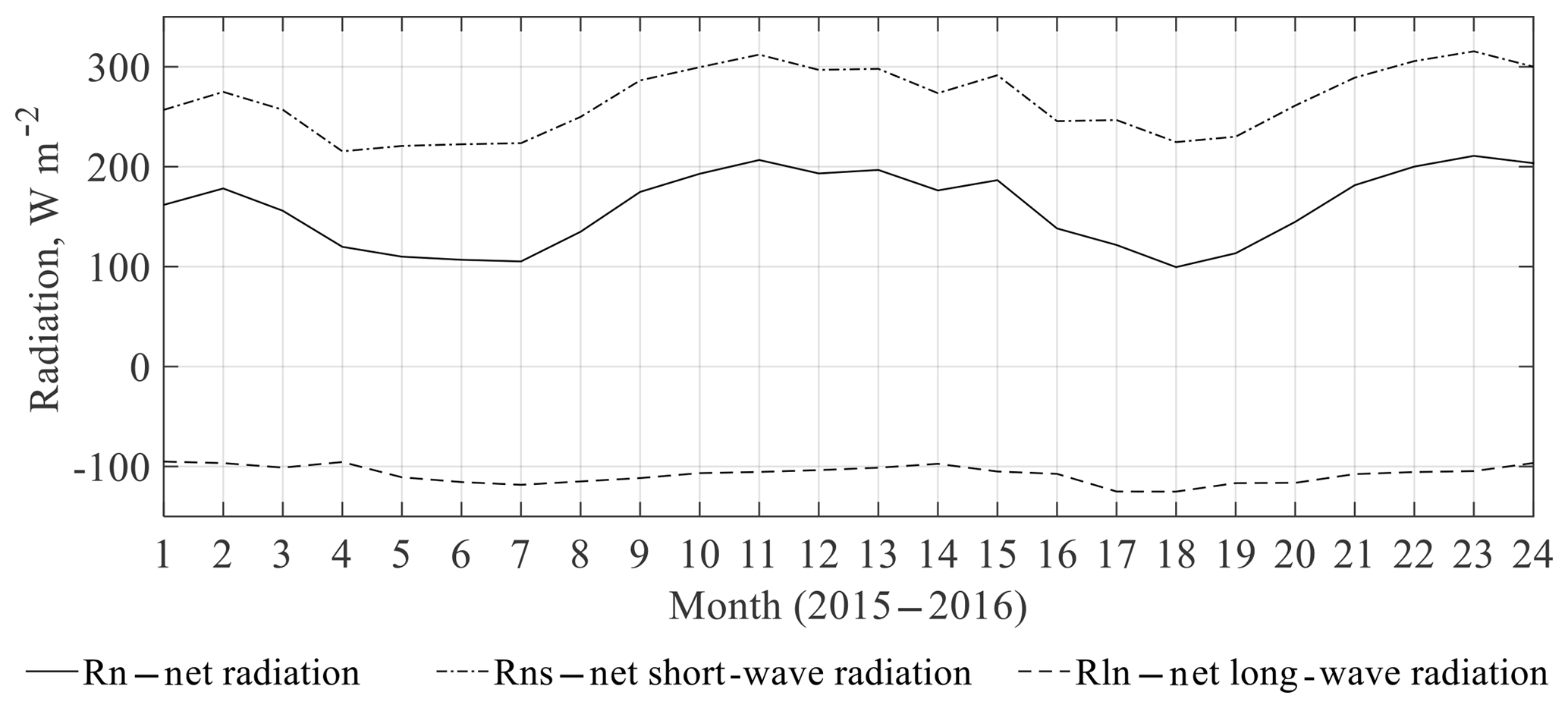
Short-wave radiation was measured, while long-wave radiation was computed as described above. The average for all components is shown in Fig. 4. The radiation budget is positive every day, with a mean of about 150 Wm⁻², varying from 100 in winter to 200 Wm⁻² in summer.

Figure 4 Monthly average radiative budget for Lake Titicaca in 2015–2016.

5 Results and discussion

5.1 Monthly data

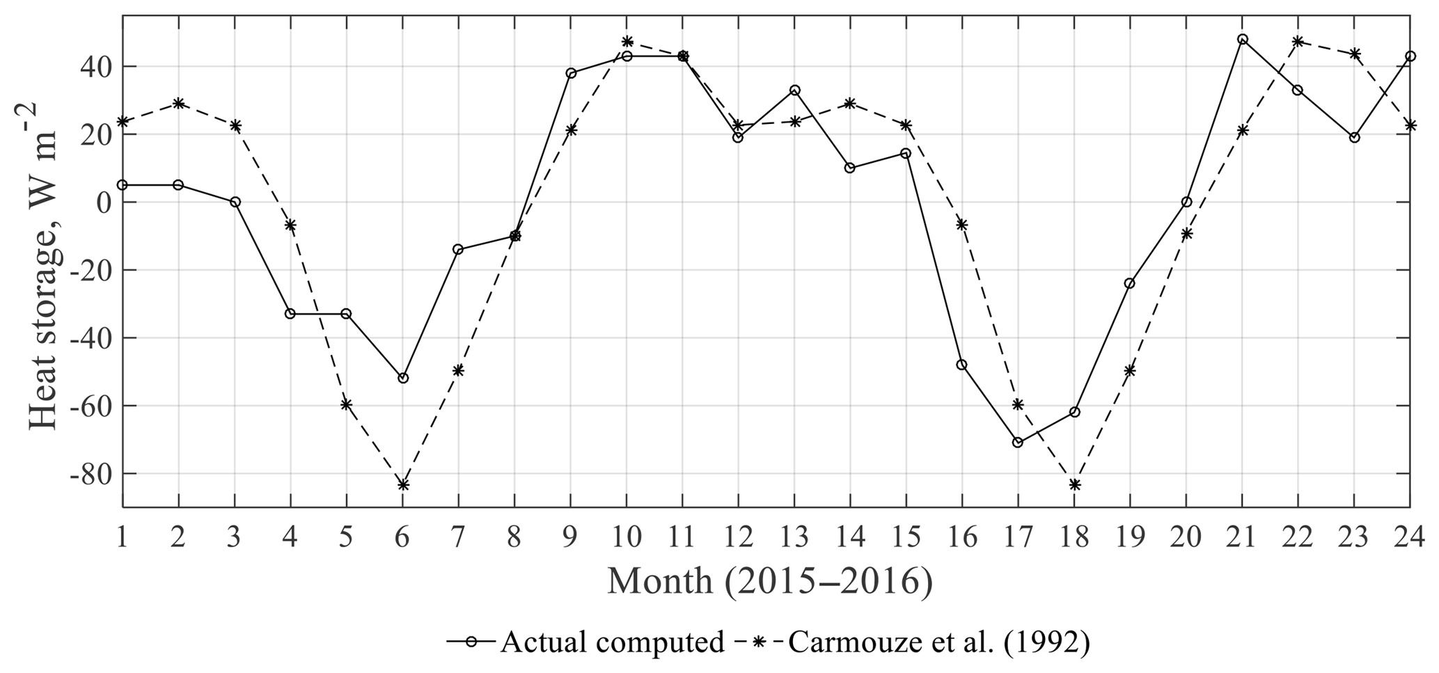
Detailed energy balance computations over the period 2015–2016 should give good estimates of the total lake evaporation for that period. After 24 months the lake surface temperature at Puno more or less returned to the temperature at the beginning of 2015. When applying this method over the 2 years of study the mean annual lake evaporation is 1700 mm year⁻¹. When computing the evaporation month by month, the change of heat storage was considered in the way previously described. The mixing depth was set to 40 m. The change of the heat storage is shown in Fig. 5. The values suggested by Carmouze et al. (1992) are shown for comparison. The calculated monthly heat storage agrees well with the Carmouze estimates.

Figure 5 Change of heat storage in 2015–2016.

The computed monthly evaporation using monthly average data and the energy balance method was somewhat higher in 2016 than in 2015, 1725 mm year⁻¹ as compared to 1680 mm year⁻¹. The small gap of evaporation between 2 consecutive years is mainly explained by the warmer season that occurred in autumn of 2015; otherwise the evaporation was fairly evenly distributed over the year, being about 140 mm month⁻¹, with somewhat lower evaporation rates from July to September (see in Fig. 6).

Figure 6 Monthly evaporation computed using energy balance approach.

From the energy balance and the water balance methods, the annual evaporation from Lake Titicaca was estimated in the range of about 1700 mm year⁻¹. The monthly variation depends on the change of heat storage, therefore the calculated evaporation may be high one month and low the following month. When using the mass transfer approach, similar annual evaporation to that from the energy balance approach may be anticipated when applying the approaches over 2 full years. This may be the case even though there may be differences when comparing monthly calculations. However, when the coefficients suggested by Carmouze et al. (1992) were used, the evaporation was much higher than 1720 mm year⁻¹, which was found from the energy balance method. A good fit for the total evaporation was found using the coefficients a=0.17 mbar and b=0.155 mm mbar⁻¹ s m⁻¹.

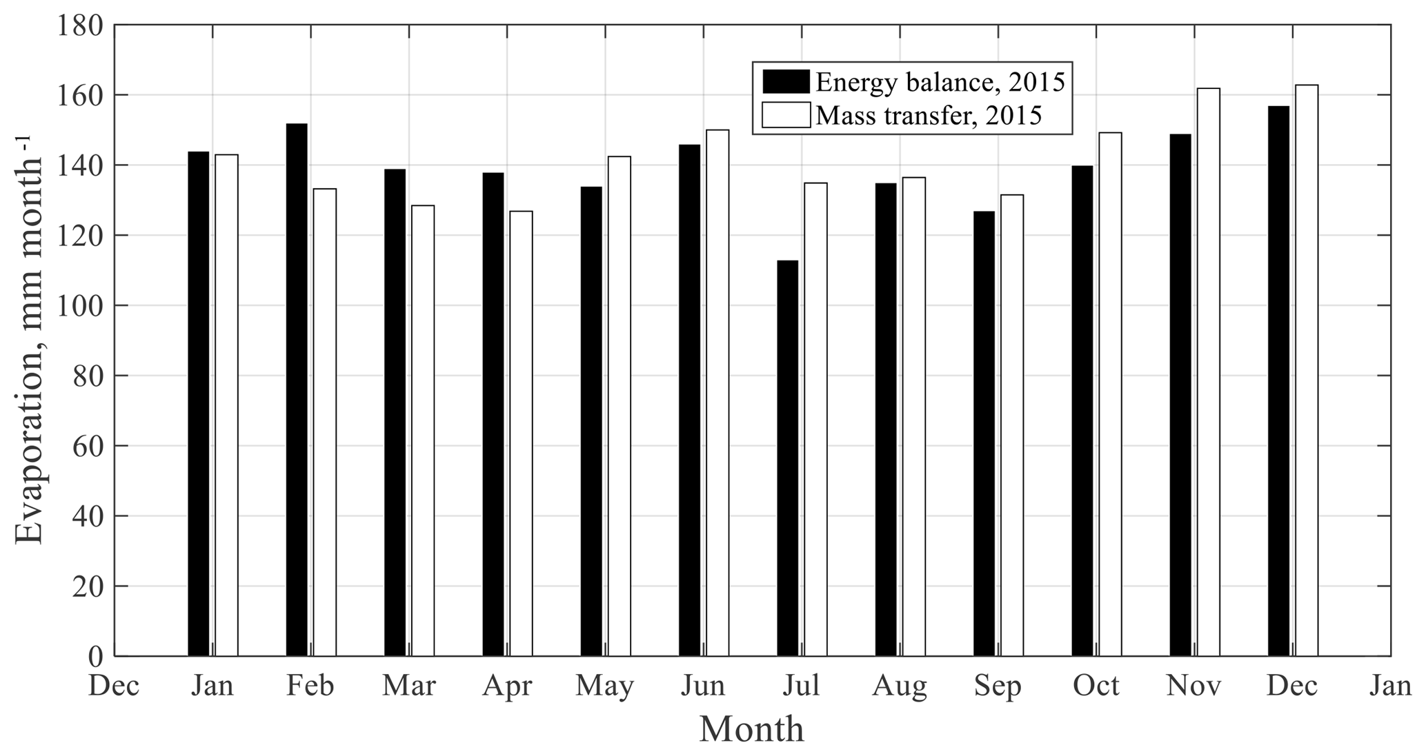
Figure 7 Comparison of monthly evaporation computed by energy balance and mass transfer method for 2015.

The monthly evaporation computed by mass transfer over the 2 years is compared with the energy balance calculations in Fig. 7 for 2015 and in Fig. 8 for 2016. The computed annual evaporation by the last method was 1700 mm year⁻¹ in 2015 and 1675 mm year⁻¹ in 2016. Consequently, for individual years the two methods gave similar results and similar seasonal trends. This is expected, since the coefficients in the mass transfer equation were chosen to fit over the 2-year period. For individual months, there are deviations. However, it is not possible to note any systematic differences related to different seasons of the year. The largest difference between the two methods for an individual month was about 30 mm.

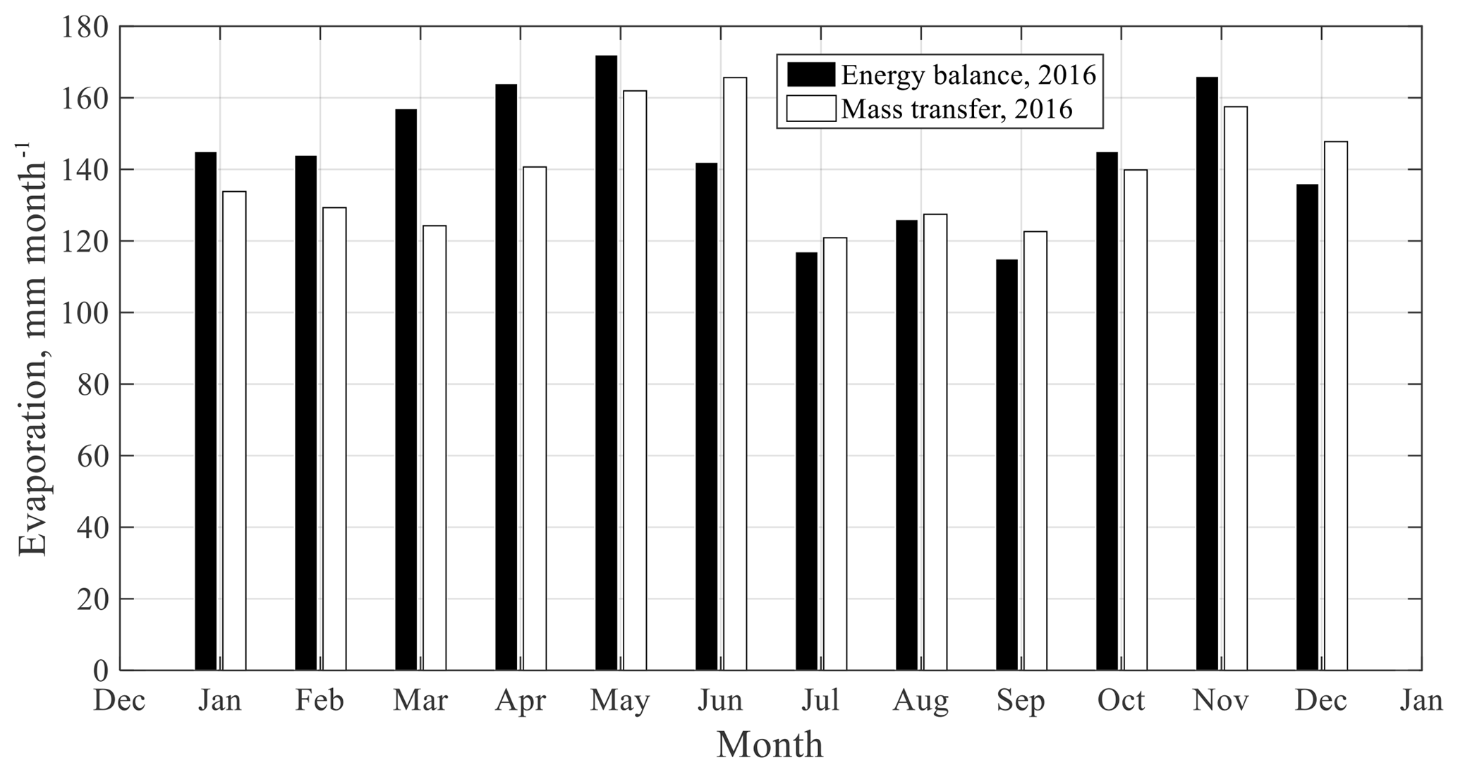
Figure 8 Comparison of monthly evaporation computed by energy balance and mass transfer method for 2016.

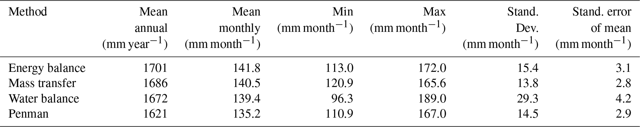
A summary and comparison of all investigated methods for the study period are shown in Fig. 9 and Table 5. As seen from these, the evaporation calculated from water balances differs from the three other methods. The water balance method yielded 1672 mm year⁻¹ as the average for the tow year. As well, the same method gave the largest standard deviation. The variation in mean annual evaporation was 1633–1711 mm year⁻¹. Since the lake water level can be observed at best with a resolution in centimetres, individual monthly evaporation becomes highly uncertain, like in February 2016 and May 2016. Thus, calculated annual evaporation is better performed using the three other methods. In general, the mass transfer, energy balance and Penman methods gave a similar monthly variation as described above; only the evaporation by Penman gave a smaller rate than the rest of models, 1621 mm year⁻¹, while energy balance gave the highest evaporation rate, 1701 mm year⁻¹.

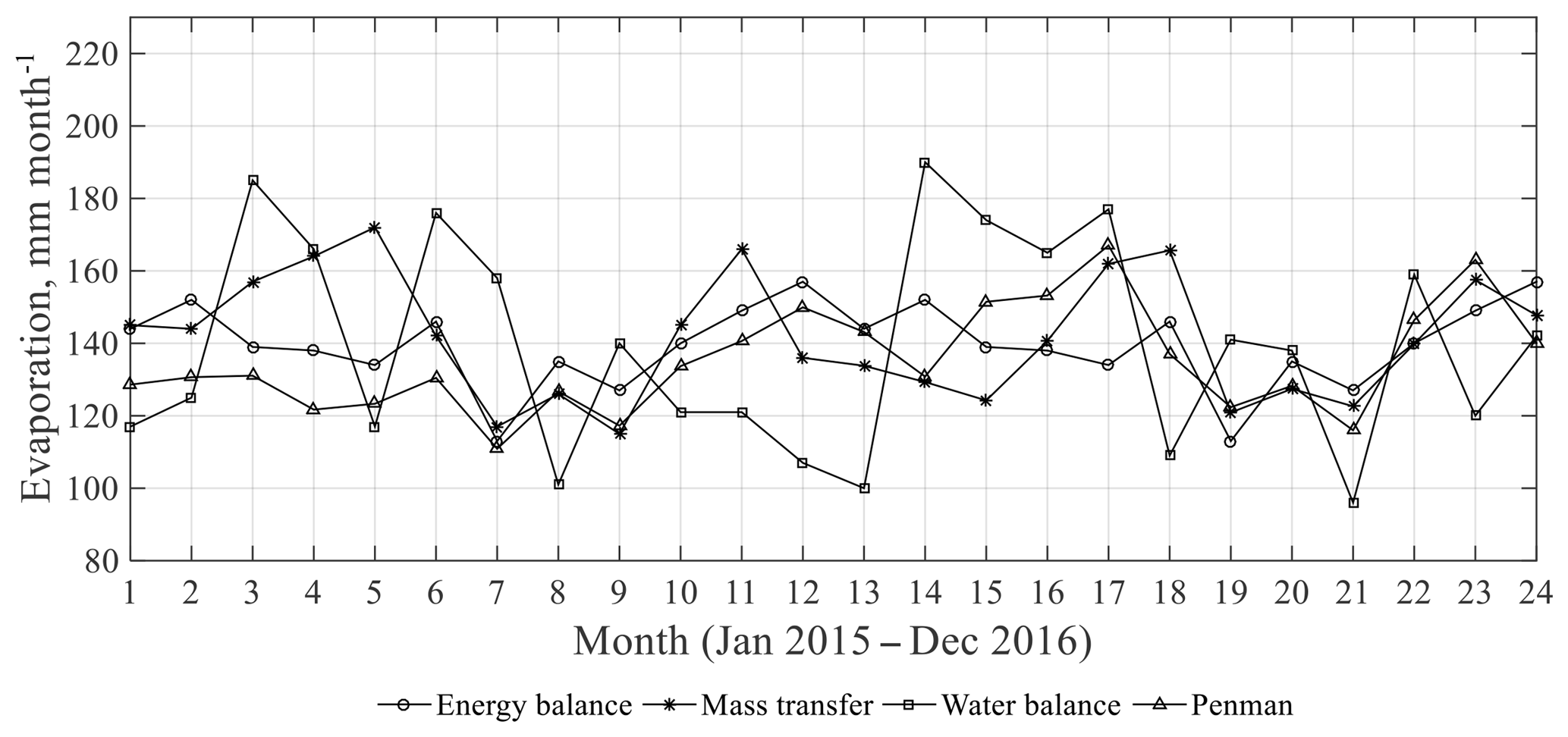
Figure 9 Monthly actual evaporation calculated by the four methods for the period from January 2015 to December 2016.

Table 5 Descriptive statistics of monthly evaporation calculated by the four methods for the period from January 2015 to December 2016.

Water balances were computed for the long-term period and continuous available data in 1966–2011 as well. During the computation the A_lake parameter in the model was assumed to be constantly equal to 8800 km². The resulting annual lake evaporation for the period 1966–2011 was about 1600 mm year⁻¹. The mean water balance components for the last period at monthly mean values are shown in Table 6. When we used the water balance approach the computed evaporation internally varied greatly from month to month and year to year. This is an indication that some hydrological input data are uncertain, like the precipitation, which can be improved from one point observation at lake shore by the satellite observation. In any case, water balance computations over a long-term period should give a reasonable estimate of mean lake evaporation.

Table 6 Monthly mean water balances for Lake Titicaca for the period 1966–2011.

5.2 Using daily data

When calculating evaporation using daily data, it was found that there are large differences between the methods and ignoring the water balance method. The maximum daily evaporation using the mass transfer method was 12 mm day⁻¹. Neither the energy balance nor the Penman method gave a higher evaporation than 8 mm day⁻¹. There was poor agreement between the computed daily evaporation computed by mass transfer and the corresponding results using the other two methods.

When the mass transfer approach is used, it is straight-forward to determine the daily evaporation. Using the energy balance, the change of heat storage in the lake must be determined with high resolution. Detailed water temperature measurements are not available, however. Instead, it was assumed that the temperature changes at a steady rate through individual months. August is an example, since the temperature for the whole month changed very little (0.2 ^∘C). The computed daily evaporation is shown for August 2015 in Fig. 10. There were 2 days with average winds exceeding 6 ms⁻¹. Consequently, the evaporation was high during these days, when the mass transfer approach was used.

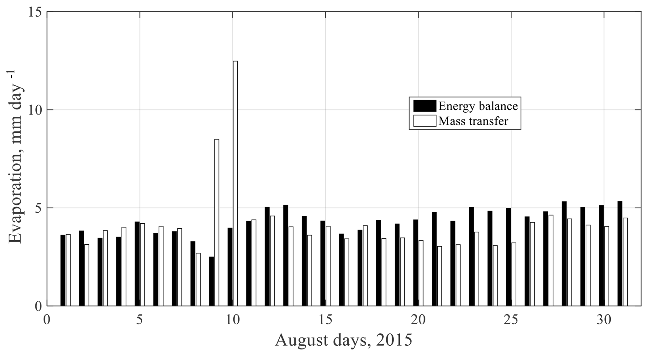
Figure 10 Daily evaporation computed by the mass transfer (shaded staples) and energy balance (filled staples) method.

When annual evaporation was determined using daily data instead of monthly mean data, there was hardly any difference for the mass transfer method. As indicated above it is not possible to use the energy balance method with short time resolution when temperature changes have to be taken in to account from day to day. However, the evaporation can be computed while neglecting the heat change, keeping the Bowen ratio constant throughout a month and changing the Bowen ratio day by day. In this case, it was found that evaporation increased by about 2 %. The conclusion, considering the many uncertainties involved in estimating evaporation, is that it is sufficient to use monthly means when estimating evaporation.

The evaporation computed with the Penman equation falls between what was found by the energy balance and the mass transfer approach, being somewhat closer to the energy balance than to the mass transfer results. Since monthly means are sufficient for computing evaporation with the two above methods, mean values are also sufficient when using the Penman method.

It has to be noted that Lake Titicaca's near-bank surface temperatures have been observed to be warmer than the lake surface's average during daytime using satellite thermal imagery, as reported in other lakes (e.g. Marti-Cardona et al., 2008). According to this observation, the temperatures acquired for this study are likely to be an overestimation.

The spatial distribution of Lake Titicaca's surface temperature and its impact on the evaporation losses is currently under analysis. However, for the energy balance method, daily changes rather than absolute temperatures were used, which are considered to be reasonable approximations of the heat storage changes. Over the larger period of air temperatures observed at the Copacabana weather station (1966–2016), the particular months in 2015–2016 have been characterized by the strongest El Niño dry phenomena during the last 50 years (http://www.ciifen.org, last access: 10 January 2017); in comparison to the rest of the years, the air temperatures recorded were higher than the average of 10 ^∘C and close to 20 ^∘C at the daily time step. Then the rates of evaporation found might express, somehow, the indicated warmer period.

6 Conclusions

Due to uncertainty of most observed data such as river inflow to Lake Titicaca, and mainly the discharge data, it might not be easy to improve the water balance results; thus it is suggested that the most reliable method of determining the lake evaporation is using the heat balance approach. To estimate the lake evaporation using this method, heat storage changes must be known. Since convection from the surface layer is intense during nights, resulting in a well-mixed top layer every morning, it is possible to determine the change of heat storage from the measured morning surface temperature. The lake evaporation is fairly uniformly distributed over the year, with lows between July and September. The mean annual evaporation is about 1700 mm year⁻¹, and the mean monthly evaporation is 141.8 mm month⁻¹. When using the mass transfer approach, the required coefficients in the aerodynamic equation was set so that the mean annual evaporation agreed with that obtained from the heat balance calculations. These coefficients were found to be lower than coefficients used in previous studies. Also, when using the mass transfer approach, the evaporation was found to be lowest in July–September.

However, for the purpose of assessing climate change effects on Lake Titicaca's evaporation, the practical approach, rather than the two empirical models, might be the Penman equation due to available observed data for this lake and the integral behaviour of the equation. Also in comparison with the two models proposed in Delclaux et al. (2007) for modelling the lake evaporation, the first model only depends on the solar radiation data, and, additionally, the second one depends on the air temperature factor; thus both models cannot be applied broadly. In the Penman model based on the adjusted wind coefficient, the mean annual evaporation is 1620 mm year⁻¹, and the mean monthly is 135 mm month⁻¹. So far, monthly evaporation computed using daily data and monthly means resulted in minor differences. The most practical model for use at the daily scale might be the mass transfer and the Penman models in comparison to the energy balance approach, which is of highly demanded observed data. Particularly the Penman equation at the daily temporal scale might correctly be applied for the climate change assessment at this altitude. Nonetheless, according to spatial available data from remote sensing, the evaporation equations used at daily and monthly scales could be applied from now on to improve the spatial pattern of the lake evaporation. Since we had really extreme single warmer days during the period 2015–2016 due to the El Niño phenomenon, higher daily rates of evaporation must be expected; therefore the application of the models at both timescales for the study period we believe that was found the upper limits of yearly evaporation.