the Creative Commons Attribution 4.0 License.
the Creative Commons Attribution 4.0 License.
 | 04 Feb 2019
Capturing soil-water and groundwater interactions with an iterative feedback coupling scheme: new HYDRUS package for MODFLOW
Jicai Zeng
Jinzhong Yang
Yuanyuan Zha
Liangsheng Shi
Accurately capturing the complex soil-water and groundwater interactions is vital for describing the coupling between subsurface–surface–atmospheric systems in regional-scale models. The nonlinearity of Richards' equation (RE) for water flow, however, introduces numerical complexity to large unsaturated–saturated modeling systems. An alternative is to use quasi-3-D methods with a feedback coupling scheme to practically join sub-models with different properties, such as governing equations, numerical scales, and dimensionalities. In this work, to reduce the nonlinearity in the coupling system, two different forms of RE are switched according to the soil-water content at each numerical node. A rigorous multi-scale water balance analysis is carried out at the phreatic interface to link the soil-water and groundwater models at separated spatial and temporal scales. For problems with dynamic groundwater flow, the nontrivial coupling errors introduced by the saturated lateral fluxes are minimized with a moving-boundary approach. It is shown that the developed iterative feedback coupling scheme results in significant error reduction and is numerically efficient for capturing drastic flow interactions at the water table, especially with dynamic local groundwater flow. The coupling scheme is developed into a new HYDRUS package for MODFLOW, which is applicable to regional-scale problems.
- Article
(5044 KB) - Full-text XML
- BibTeX
- EndNote


Numerical modeling of the soil-water and groundwater interactions has to deal with flow components and governing equations at different scales. This adds significant complexity to model development and calibration. Unsaturated soil-water and saturated groundwater flows with similar properties are usually integrated into a whole modeling system. Although physically consistent and numerically rigorous, methods involving the 3-D Richards' equation (RE; Richards, 1931) tend to be computationally expensive and numerically unstable due to the large nonlinearity and the demand for dense discretization (Kumar et al., 2009; Maxwell and Miller, 2005; Panday and Huyakorn, 2004; Thoms et al., 2006; Zha et al., 2013a), especially for problems with multi-scale properties. In this work, parsimonious approaches, which appear in different governing equations and coupling schemes, are developed for modeling the soil-water and groundwater interactions at regional scales.
Simplifying the soil-water flow details into upper flux boundaries has been widely used to simulate large-scale saturated flow dynamics, such as the MODFLOW package and its variants (Langevin et al., 2017; Leake and Claar, 1999; McDonald and Harbaugh, 1988; Niswonger et al., 2011; Panday et al., 2013; Zeng et al., 2017). At the local scale, in contrast, the unsaturated flow processes are usually approximated with reasonable simplifications and assumptions in RE (Bailey et al., 2013; Liu et al., 2016; Paulus et al., 2013; Šimůnek et al., 2009; van Dam et al., 2008; Yakirevich et al., 1998; Zha et al., 2013b).
The original RE, also known as the mixed-form RE, takes the pressure head (h) as the driving force variable, while soil moisture content (θ) is the mass accumulation variable (Krabbenhøft, 2007). To solve the mixed-form RE, either h or θ, or a switching of both, is assigned as the primary variable. The h-form RE is widely employed for unsaturated–saturated flow simulation, especially in heterogeneous soils, such as the HYDRUS package (Šimůnek et al., 2016). Significant improvement in mass conservation has been achieved with Celia's modification (Celia et al., 1990). Then, efforts were made to combine the advantages in the original and the Celia-format h-form REs by switching their storage terms (Hao et al., 2005; Zadeh, 2011). However, these models still suffer from a high computational cost and low numerical robustness when dealing with rapidly changing atmospheric boundary conditions (Crevoisier et al., 2009; Zha et al., 2017). The θ-form RE, addressing the above problems, is inherently mass conservative and less nonlinear in the averaged nodal hydraulic diffusivity when the soil is dry (Warrick, 1991; Zha et al., 2013b). However, the θ-form RE is not applicable to saturated and heterogeneous soils (Crevoisier et al., 2009; Zha et al., 2013b). In this work, to take advantage of both forms of RE, the governing equations, rather than primary variables (Diersch and Perrochet, 1999; Forsyth et al., 1995; Zha et al., 2013a), are switched at each node according to its saturation degree.
For regional problems, the vadose zone is usually conceptualized into paralleled soil columns without lateral connections. The resulting quasi-3-D coupling scheme (Kuznetsov et al., 2012; Seo et al., 2007; Xu et al., 2012; Zhu et al., 2012) significantly reduces the dimensionality and complexity. According to how the messages are transferred across the coupling interface, the quasi-3-D methods are categorized into (1) the fully coupling scheme, which simultaneously builds the nodal hydraulic connections of sub-models at both sides and implicitly solves the assembled matrices; (2) the one-way coupling scheme, which delivers the soil-water model solutions onto the groundwater model without feedback mechanism; and (3) the feedback (or two-way) coupling scheme, which explicitly exchanges the head and/or flux solutions in vicinity of the interface nodes.
The fully coupling scheme (Gunduz and Aral, 2005; Zhu et al., 2012) is numerically rigorous but tends to increase the computational burden under practical conditions. For example, the potentially conditional diagonal dominance causes non-convergence for the iterative solvers (Edwards, 1996). Owing to high nonlinearity in the soil-water sub-models, the assembled matrices can only be solved with unified small time steps, which adds to the computational expense. The one-way coupling scheme, as adopted by the UZF1 package for MODFLOW (Grygoruk et al., 2014; Niswonger et al., 2006) as well as the free drainage mode in SWAP package for MODFLOW (Xu et al., 2012), assumes that the water-table depth has a minor influence on flow interactions at the phreatic interface and is thus problem specific.
The feedback coupling methods, in contrast, are widely used (Kuznetsov et al., 2012; Seo et al., 2007; Shen and Phanikumar, 2010; Stoppelenburg et al., 2005; Xie et al., 2012; Xu et al., 2012) as a compromise of numerical accuracy and computational cost. In a feedback coupling scheme, the soil-water and groundwater sub-models can be built with governing equations and numerical schemes at different scales. For flow processes with multi-scale components, such as boundary geometries, parameter heterogeneities, and hydrologic stresses, the scale-separation strategy can be implemented easily. Although the feedback coupling method is numerically more rigorous than a one-way coupling method, and tends to reduce the inconsistency of head and/or flux interfacial boundaries, some concerns arise.
The first concern is the numerical efficiency of the iterative and non-iterative feedback coupling methods. The non-iterative approach (Twarakavi et al., 2008; Xu et al., 2012) usually leads to significant error accumulation when dealing with a dynamically fluctuating water table, especially with large time-step sizes. The iterative methods, in contrast (Kuznetsov et al., 2012; Stoppelenburg et al., 2005; Xie et al., 2012), by converging the head and/or flux solutions at the coupling interface, are numerically rigorous but computationally expensive, especially when solving the coupled sub-models with a unified time-stepping scheme (Kuznetsov et al., 2012). Good balance between cost and effect is needed to maintain practical utility of the iterative feedback coupling scheme.
The second concern lies in the scale-mismatching problem. For groundwater models (Harbaugh et al., 2005; Langevin et al., 2017; Lin et al., 2010; McDonald and Harbaugh, 1988), the specific yield at the phreatic surface is usually represented by a simple large-scale parameter, while for soil-water models (Niswonger et al., 2006; Šimůnek et al., 2009; Thoms et al., 2006), the small-scale phreatic water release is influenced by the water-table depth and the unsaturated soil moisture profile (Dettmann and Bechtold, 2016; Nachabe, 2002). Delivering small-scale solutions of the soil-water models onto the large-scale interfacial boundary of the groundwater model, as well as maintaining the global mass balance, usually introduces significant nonlinearity to the entire coupling system (Stoppelenburg et al., 2005). Conditioned by this, the mismatch of numerical scales in the coupled sub-models causes significant coupling errors and instability. A multi-scale water balance analysis at the phreatic surface helps to relieve such difficulties.
The third concern is the nontrivial lateral fluxes between the saturated regions controlled by the vertical soil columns, which are usually not considered in previous study (Seo et al., 2007; Xu et al., 2012). Though rigorous water balance analysis is conducted to address such inadequacy (Shen and Phanikumar, 2010), the lateral fluxes solved with a 2-D groundwater model usually require additional efforts to build water budget equations in each subdivision represented by the soil columns. A moving-boundary strategy helps to avoid the saturated lateral flow in the groundwater body.
In this work, the h- and θ-form of the 1-D RE are switched at the equation level to obtain a new HYDRUS package. To handle three of the aforementioned concerns, a multi-scale water balance analysis is carried out at the phreatic surface to conserve head and/or flux consistent at the coupling interface. An iterative feedback coupling scheme is developed for linking the unsaturated and saturated flow models at disparate scales. The saturated lateral fluxes between the soil columns are fully removed from the interfacial water balance equation, making it a moving-interface coupling framework. The head solution of MODFLOW 2005 (Harbaugh et al., 2005; Langevin et al., 2017) and flux solution of HYDRUS-1D (Šimůnek et al., 2009) are relaxed to meet consistency at the phreatic surface.
In this paper, the governing equations at different scales, the multi-scale water balance analysis at the phreatic surface, and the iterative feedback coupling scheme for solving the whole system, are presented in Sect. 2. Synthetic numerical experiments are described in Sect. 3. Numerical performance of the developed model is investigated in Sect. 4. Conclusions are drawn in Sect. 5.
To address the aforementioned first concern, governing equations for subsurface flow are given at different levels of complexity (Sect. 2.1), numerical solutions of these equations are presented (Sect. 2.2), and nonlinearity in the soil-water sub-models is reduced by a generalized switching scheme that chooses appropriate forms of RE according to the hydraulic conditions at each numerical node (Sect. 2.3). Then, an iterative feedback coupling scheme is developed to solve the soil-water and groundwater models at independent scales (Sect. 2.4). As for the second concern, a multi-scale water balance analysis is conducted to deal with the scale-mismatching problem at the phreatic surface (Sect. 2.5). To cope with the third concern, a moving Dirichlet boundary at the groundwater table is assigned to the soil-water sub-models (see Appendix Sect. A1); the Neumann upper boundary for the saturated model is provided in Sect. A2, and the relaxed iterative feedback process is presented in Sect. A3.
2.1 Governing equations
The mass conservation equation for unsaturated–saturated flow is given by
where t is time (T); θ (L3 L−3) is volumetric moisture content; h (L) is the pressure head; β is 1 for the saturated region but zero for the unsaturated region; C (L−1) is the soil-water capacity () for the unsaturated region but zero for saturated region; μs (L−1) is the specific elastic storage; and q (L T−1) is the vector for Darcian flux calculated by the following:
where K (L T−1) is the hydraulic conductivity, K=K(θ), and H (L) is the potentiometric head, , in which z is the vertical location with a coordinate positive upward. Combining Eqs. (1) and (2) results in the governing equation for groundwater flow,
With the assumption that the horizontal unsaturated flows are negligible, the regional vadose zone is usually represented by an assembly of paralleled soil columns. The generalized 1-D RE is represented by a switchable format,
where ψ is the primary variable. For an h-form RE, ψ=h, , and , while for a θ-form RE, ψ=θ, , and ; where D (L2 T−1) is the hydraulic diffusivity, .
2.2 Numerical approximation
The governing equation for the saturated zone (Eq. 3) is spatially and temporally approximated in the same form as the MODFLOW 2005 model (Harbaugh et al., 2005; Langevin et al., 2017). Celia's modification (Celia et al., 1990; Šimůnek et al., 2009) is applied to the h-form 1-D RE for temporal approximation. Both forms of RE are handled with a temporally backward finite difference discretization (Zha et al., 2013b, 2017). Each sub-model is solved by a Picard iteration scheme, which is widely used in some popular codes or software packages (van Dam et al., 2008; Šimůnek et al., 2016).
The spatial discretization of Eq. (4), as well as the water balance analysis for each node, is based on the nodal flux in element (bounded by nodes i and i+1), which is
where the superscripts j and k are the levels of time and inner iteration, the subscript i (or ) is the number of node (or element), and is the length of the element , . When a soil interface exists at node i, for example, the soil moisture contents in elements and are discontinuous at node i, thus dissatisfying the θ-form RE. To address this problem, the correction term , suggested by Zha et al. (2013b), is employed to handle the heterogeneous interface at nodes i and i+1,
where variables (scalar) and are the continuously distributed ψ within element , i.e., between the vertices i and i+1.
When ψ=h, or when ψ=θ, but no heterogeneity occurs, we get and , so . When ψ=θ, with soil interfaces at node i or i+1, and . It is obvious that (or , so .
Hereinafter, represents the soil parameters in element . For example, in a van Genuchten model (van Genuchten, 1980), (θr, θs, n, m, α, ks), where θr (L3 L−3) and θs (L3 L−3) are the residual and saturated soil moisture contents; α (L−1), n, and m are the pore-size distribution parameters, ; and ks (L T−1) is the saturated hydraulic conductivity.
2.3 Switching Richards' equation
Due to lower nonlinearity of hydraulic diffusivity (D) for dry soils (Zha et al., 2013b) and the avoidance of the mass balance error by removing the soil-water capacity in the storage term, the θ-form RE is more robust than the h-form RE, especially when dealing with rapidly changing atmospheric boundary conditions (Zeng et al., 2018). In our work, the h- and θ-form REs are switched at each node according to its effective saturation, Se. The resulting hybrid matrix equation set is solved by the Picard iteration. The empirical effective saturation for doing switching varies with soil type and is suggested to be Secrit=0.4–0.9, the state when both the h- and θ-form REs are stable and efficient. When Se ≥ Secrit, the soil moisture is closer to saturation, so the h-form RE is chosen as the governing equation; otherwise, when it undergoes dry soil condition, the θ-form RE is preferred.
For element , when the governing equations for nodes i and i+1 are identical, the spatial approximation of nodal flux is given by Eq. (5). When the governing equations differ at nodes i and i+1, a switched element is produced. When taking ψi=θi and as an example, the nodal fluxes calculated by Eq. (5) for different forms of RE have to be carefully handled by substituting with , while is replaced by . When ψi=hi and , in contrast, is replaced by , while is replaced by . The resulting equivalent nodal fluxes and are then weighted to obtain an approximation by
where ω is the weighting factor, . In our work, ω=0.5 is applied to implicitly maintain the unknown variables of both and . Specifically, when ω=1, the h-form RE is used at nodes i and i+1; when ω=0, the θ-form RE is employed instead. A detailed study on the switching of RE between two ends of the soil moisture condition, as well as the description of the numerical formation, can be found in Zeng et al. (2018).
Note that the equation switching method takes full advantage of the θ- and h-form REs, which is different from the traditional primary variable switching schemes (Diersch and Perrochet, 1999; Forsyth et al., 1995; Zha et al., 2013a). In our work, the switching-RE approach is incorporated into a new HYDRUS package.
2.4 Iterative feedback coupling scheme
The Dirichlet and Neumann boundaries are iteratively transferred across the phreatic interface. The groundwater head solution serves as the head-specified lower boundary of the soil columns, while the unsaturated solution is converted into the flux-specified upper boundary of the groundwater model. Due to moderate variation of the groundwater flow, the predicted water-table solution is usually adopted in advance as the Dirichlet lower boundary of the fine-scale soil-water flow models (Seo et al., 2007; Shen and Phanikumar, 2010; Xu et al., 2012), which in sequence then provides the Neumann upper boundary for successively solving the coarse-scale groundwater flow model. Section A1 provides the method for a moving Dirichlet lower boundary, while Sect. A2 presents the Neumann upper boundary for the 3-D groundwater model. In Sect. A3, the relaxed iterative feedback coupling scheme is used to solve the unsaturated–saturated sub-models at two sides of the coupling interface.
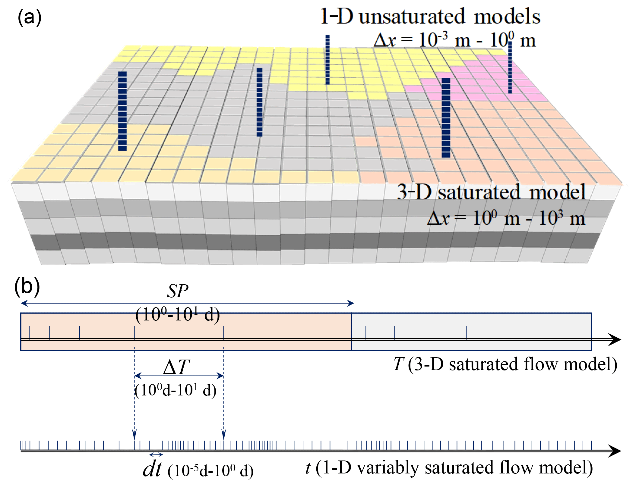
Figure 1Schematic of the space- and time-splitting strategy for coupling models at two independent scales. For a groundwater model, spatial discretization is expected to be large (Δx=100– 103 m), while for soil-water models, it is small (–100 m). Multiple levels of temporal discretization are common for regional problems. For the groundwater model, the stress periods (SP) and macro-time-step sizes (ΔT) appear in months and days (100–101 days). For soil-water models, the time-step sizes are about 10−5–100 days.
2.5 Multi-scale water balance analysis
Coupling models at different scales requires consistency in their spatial and temporal scales at the interface (Downer and Ogden, 2004; Rybak et al., 2015). A space- and time-splitting strategy (see Fig. 1) is adopted to separate sub-models at different scales. That is, the soil-water models are established by –100 m and –100 days, while for the saturated model, the grid sizes are Δx=100–103 m, and time-step sizes are Δt=100–101 days. Water balance at one side of the interface is conserved by scale matching of boundary conditions provided by the sub-model on the other side. For unsaturated flow, Richards' equation requires fine discretization of space and time (Miller et al., 2006; Vogel and Ippisch, 2008), while for saturated flow, coarse spatial and temporal grids produce adequate solutions at a large scale (Mehl and Hill, 2004; Zeng et al., 2017). To approximate the upper boundary flux of the groundwater flow model, a multi-scale water balance analysis is conducted within each step of the large-scale saturated flow model. At small spatial and temporal scales, e.g., within a macro-time step and at a local area of interest (with thickness of , where zs and zs are defined in Sect. A2), the specific storage term in Eq. (1) is vertically integrated into a transient one-dimensional expression (Dettmann and Bechtold, 2016),
where w (L) is the amount of unsaturated water in the moving balancing domain (see Fig. 2b), ; is the total fluctuation of the phreatic surface during , and the subscript t in zt here means the groundwater table; and θs is the saturated soil-water content. Approaching a transient state at time t, the water balance in a moving water balancing domain (see ) in Fig. 2b) during a small-scale time step dt (defined in Fig. 1b) is given by
where qtop(t) and qbot(t) (L T−1) are the nodal fluxes into and out of the moving balancing domain at a fixed top boundary (zs) and a moving bottom boundary (zb= min(, i.e., and (positive into the balancing domain and negative outside); d is the transient fluctuation of the phreatic surface during dt; and l (T−1) is the saturated lateral flux into the balancing domain at time t (see Fig. 2b). Taking Γ as the lateral boundary of a sub-domain, the lateral flux is supposed to be constant during ΔT; Ω is the volume of the saturated domain controlled by a soil column, which is horizontally projected into Π. Temporally integrating Eq. (9) from time TJ to TJ+1 produces
where Rtop (L) is the cumulative water flux at zs, . Note that Rtop equals Ftop in Eq. (A3) (Sect. A2). Rbot (L) is the cumulative water flux out of the moving balancing domain, . εl (L) is the cumulative lateral input water into the moving balancing domain,
where N is the number of time steps for the small-scale soil-water model within a macro-time step ΔT, and is the nontrivial saturated later flux produced by a stationary-boundary method (Seo et al., 2007; Xu et al., 2012). By taking Rtop as the specific recharge at zs, the small-scale specific yield is derived from Eqs. (8) and (10) as
Supposing that zt is linearly fluctuating in time, i.e., b (where a and b are constants), we get the water-table change during a small-scale step (dt) by d; thus, εl=o(dt2), which means that linearly refining the local time-step size (dt) in the soil-water model brings about at least quadratic approximation of εl towards zero. Thus εl can be neglected from the small-scale mass balance analysis. In the developed model, the large-scale specific yield, in Eq. (A3), represents the water release in the phreatic aquifer, while the small-scale in Eq. (12) denotes the dynamically changing water yield caused by the fluctuation of the water table. The upper boundary flux Ftop in the phreatic flow equation (Eq. A3) is therefore corrected to
Differing from previous studies (Seo et al., 2007; Shen and Phanikumar, 2010; Xu et al., 2012), a scale-separation strategy is employed in Eq. (13). The specific yields at two different scales are explicitly linked in Ftop. The large-scale properties in the groundwater model (MODFLOW) are thus fully maintained.
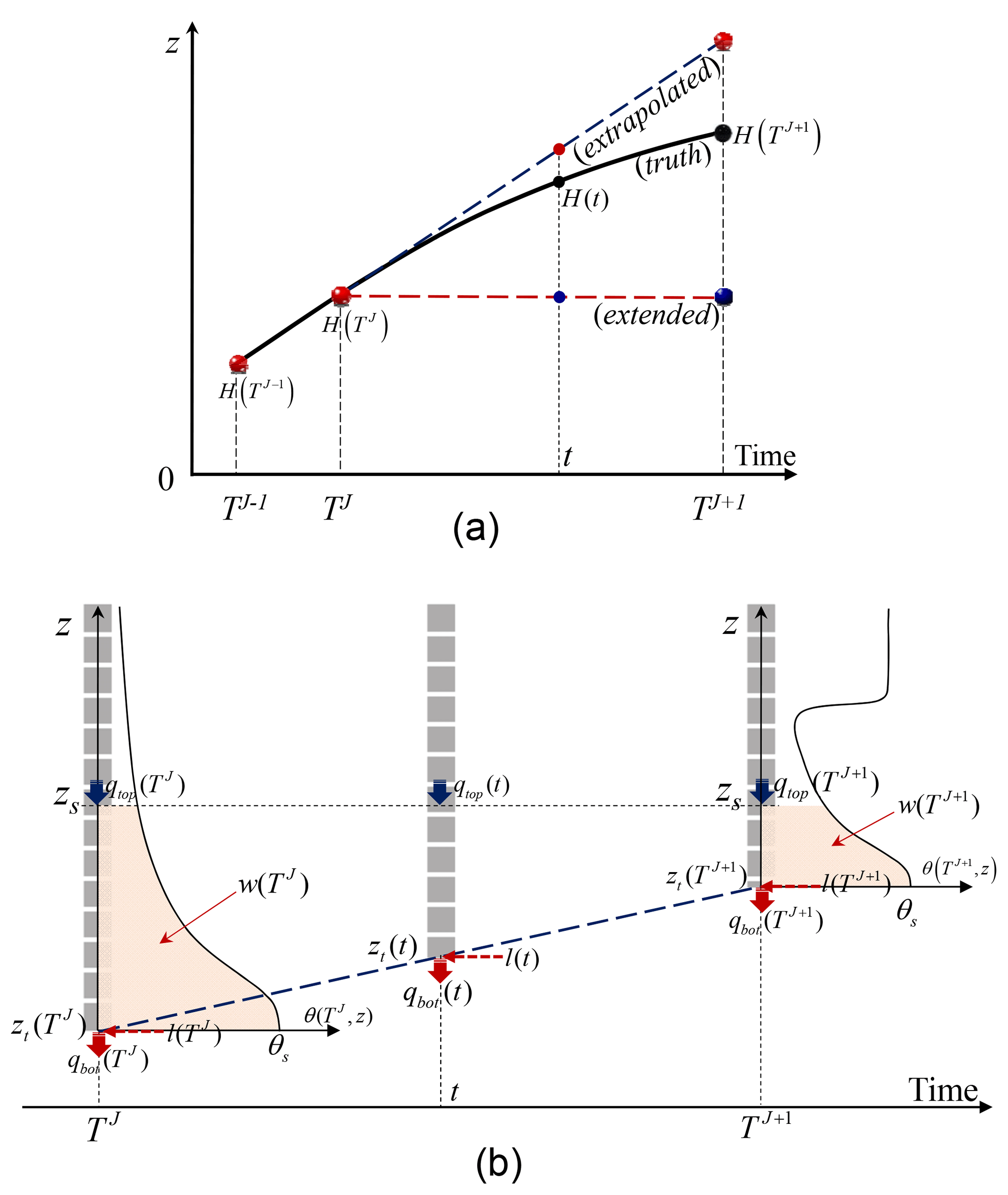
Figure 2The Dirichlet–Neumann coupling of the soil-water and groundwater flow models at different scales. (a) Linear or stepwise prediction of Dirichlet lower boundary for the soil-water flow model. (b) Water balance analysis based on a balancing domain with moving lower boundary. Blue dashed line is the linearly extrapolated groundwater table as an alternative for prediction of Dirichlet lower boundary. J (or j), T (or t), and ΔT (or dt) are the time level, time, and time-step size at coarse (or fine) scale. At any of the transient states (t), the balancing domain is bounded by a user-specified top elevation (zs) and the moving phreatic surface (zt). At a transient time t (or TJ), the total mass volume in the moving balancing domain is indicated by w(t) (or w(TJ)). The saturated lateral flux of the moving domain is indicated by l(t), while the unsaturated lateral flux is neglected as the assumption of quasi-3-D models. The water flux into and out of the balancing domain is indicated by qtop and qbot.
In this section, a range of 1-D, 2-D, 3-D, and regional numerical test cases are presented. The 1-D tests are benchmarked by the globally refined solutions from the HYDRUS-1D code (Šimůnek et al., 2009). The 2-D and 3-D “truth” solutions are obtained from the fully 3-D variably saturated flow (VSF; Thoms et al., 2006) model. At the regional scale, a synthetic case study suggested by Twarakavi et al. (2008) is reproduced. The codes are run on a personal computer with a 16 GB RAM and 3.6 GHz Intel Core (i3-4160). A maximal number of feedback iterations is set at 20. Soil parameters for the van Genuchten model (van Genuchten, 1980) are given in Table 1. The root-mean-square error (RMSE) of the solution ψ at time t is given by
where ψ is the numerical solution of either the pressure head or water content, ψref is the corresponding reference solution, and subscript i is the number of nodes, i=1, 2, …, N.

3.1 Case 1: rapidly changing atmospheric boundaries
The 1-D case is used to investigate the benefit brought by switching Richards' equation in the unsaturated zone. A soil column is initialized with a hydrostatic water-table depth of 800 cm. That is, cm, with z=0 at the bottom and z=1000 cm on the top. The lower boundary is set to non-flux to avoid the extra computational burden caused by variation of the groundwater model. Two scenarios from literature are reproduced with rapidly changing upper boundaries, as well as extreme flow interactions between the unsaturated and saturated zones.
Miller et al.'s problem (Miller et al., 1998) is reproduced in scenario 1. A dry sandy soil column (see soil no. 1 in Table 1) experiences a large constant flux infiltration at the soil surface of qtop=30 cm days−1, which ceases at t=4 days.
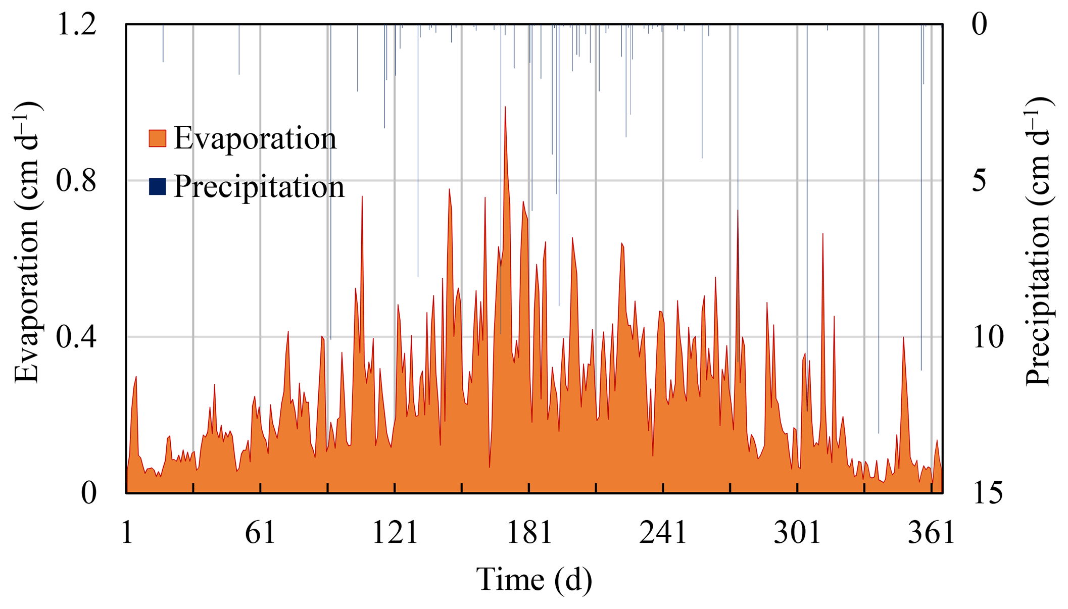
In scenario 2, Hills et al.'s problem (Hills et al., 1989) is considered. The soils no. 2 and no. 3 from Table 1 are alternatively layered with a thickness of 20 cm within the first 80 cm of depth. Below 80 cm (z=0–920 cm) is soil no. 2, with a non-flux bottom boundary. The atmospheric upper boundary conditions, rainfall and evaporation, change rapidly with time (see Fig. 3), over 365 days.
The coupled unsaturated model is discretized into a fine grid with Δz=1 cm, while the saturated model is discretized into two layers with thickness of 500 cm. The impact of different numbers of feedback iteration, closure criteria, and different forms of the 1-D Richards' equation are investigated. Solutions obtained from the HYDRUS-1D model with Δz=1 cm and Δt=0.05 days are taken as the truth.
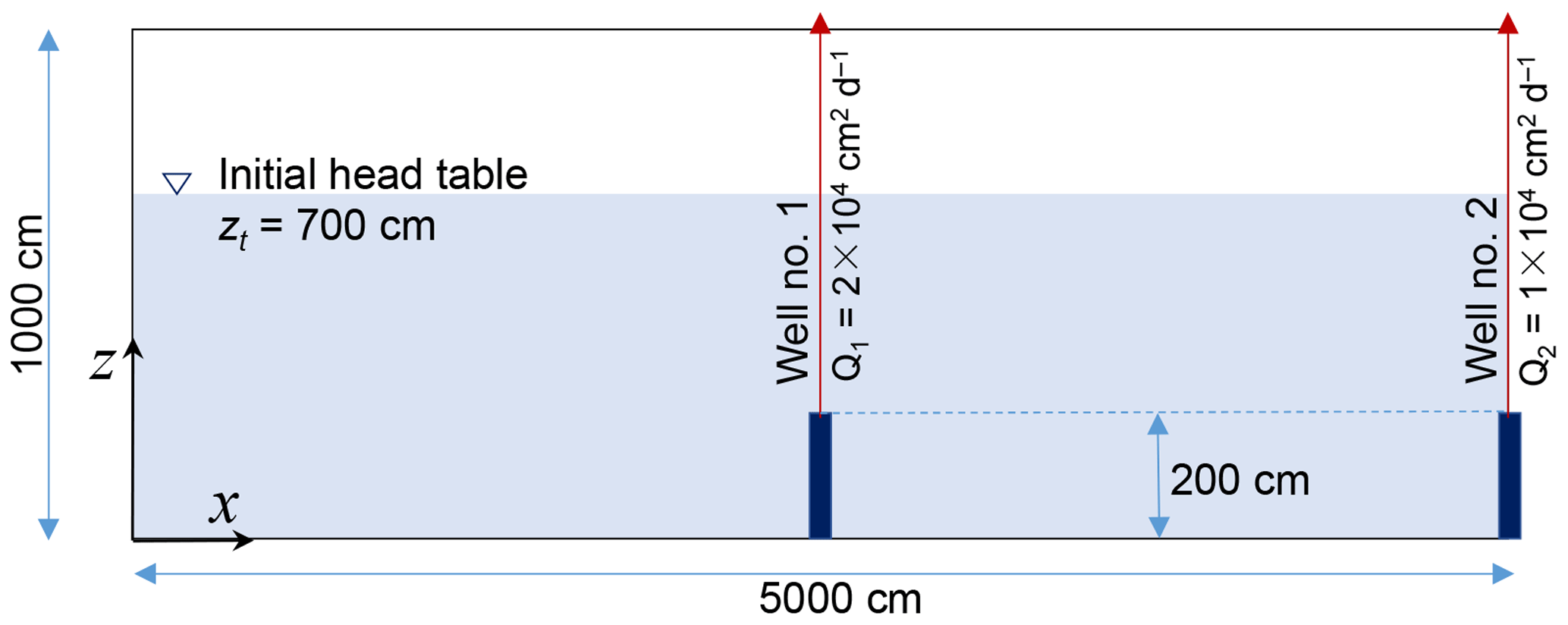
Figure 4Schematic of the cross section for test case 2. Two pumping wells with screens of z=0–200 cm are located at x=2500 and 5000 cm. The pumping rates per unit width at well no. 1 and no. 2 are 2×10⁴ and 1×104 cm2 days−1, respectively.
3.2 Case 2: dynamic groundwater flow
A 2-D case is analyzed with sharp groundwater flow (see Fig. 4). To minimize the unsaturated lateral flow, the soil surface is set with a non-flux boundary. The bottom and lateral boundaries are also non-flux. Two pumping stresses are applied to the cross-sectional field with cm ×1000 cm. Well no. 1 is located at x=2500 cm, with a pumping screen at z=0–200 cm, while well no. 2 is at x=5000 cm, with a pumping screen of z=0–200 cm. Pumping rates for wells no. 1 and no. 2 respectively are 2×10⁴ and 1×104 cm2 days−1 per unit width. The initial hydrostatic head of the cross section is cm. Soil no. 4 in Table 1 fills the entire cross section. The total simulation lasts 50 days. For the coupled saturated sub-model, as well as the reference model (VSF Thoms et al., 2006), the cross section is discretized horizontally into uniform segments with a width Δx=50 cm, while vertically (bottom up) refined into segments with thicknesses Δz=200 cm(×1), 100 cm(×2), 50 cm(×2), 25 cm(×2), 12.5 cm(×4), and 5 cm(×200), where the subscripts hereinafter (×N) are the numbers of discretized segments. The 1-D soil-water models are discretized with a segmental thickness of Δz=1 cm. The fully 2-D unsaturated–saturated solutions from the VSF model are taken as the truth.

Figure 5Different number of subzones partitioned for the quasi-3-D simulations in case 3. The vadose zone is partitioned into 16, 12, 9, 5, and 3 subzones.
3.3 Case 3: pumping and irrigation
Case 3 is used to investigate the efficiency and applicability of a quasi-3-D coupling model in comparison of the fully 3-D approaches. A phreatic aquifer with m ×1000 m ×20 m is stressed by constant irrigation and pumping wells. The infiltration rate is 3 mm days−1 in (x, y) = (0–440 and 560–1000 m), while it is 5 mm days−1 in (x, y) = (560–1000 and 0–440 m). Screens for three of the pumping wells are located at (x, y, and z) = (220, 220, and 5–10 m), (500, 500, and 5–10 m), and (780, 780, and 5–10 m). The pumping rates are constant at 30 m3 days−1. The initial hydrostatic head of the aquifer is 18 m. Around and below the aquifer are non-flux boundaries. The aquifer is horizontally discretized with m for the coupled saturated model as well as for the VSF model to obtain the truth solution. The top-down thicknesses of the fully 3-D grid are Δz=0.10 m(×30), 0.4 m(×5), 1 m(×5), and 2 m(×5). For the 1-D soil columns, they are Δz=0.1 m(×30) and 0.4 m(×5), which means that no soil column reaches the bottom. Different numbers of the subzones represented by soil columns, as well as their different geometries, are given in Fig. 5. The soil parameters for a sandy loam (soil no. 5) are given in Table 1. The total simulation lasts 60 days.
Table 2The precipitation, evaporation, and pumping rates in 12 stress periods.
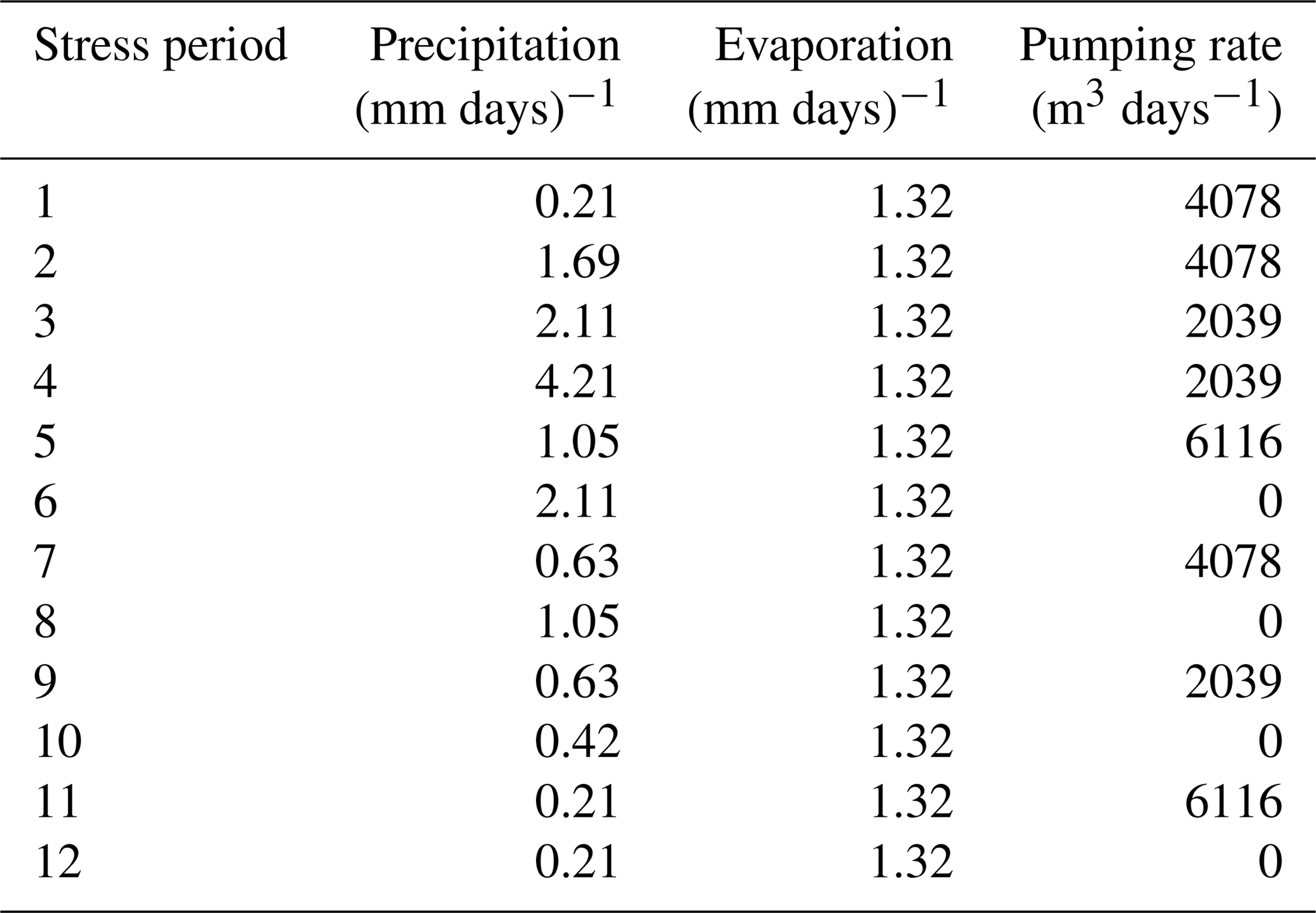
3.4 Case 4: synthetic regional case study
A hypothetical test case from literature (Niswonger et al., 2006; Prudic et al., 2004; Twarakavi et al., 2008) for a large-scale simulation is reproduced here. The overall alluvial basin is divided into uniform grids with m. The coupled saturated model is conceptualized into a single layer. The initial head, as well as the elevations of land surface and bedrock, are presented in Fig. 6a, b, and c. The precipitation, evaporation, and pumping rates for 12 stress periods, each lasting 1∕12 of 365 days, are given in Table 2. The infiltration factors (see Fig. 6d) are used to approximate the spatial variability of precipitation. The initial head in the vadose zone is set with hydrostatic status. Twenty soil columns, coinciding with the subzones in Fig. 6d, are discretized separately with a range of gradually refined segments with a thickness (Δz) from 30.48 to 0.3048 cm (bottom up). A comparative analysis is conducted with the solutions obtained from the original HYDRUS package for MODFLOW (taken as HPM for short; Seo et al., 2007).
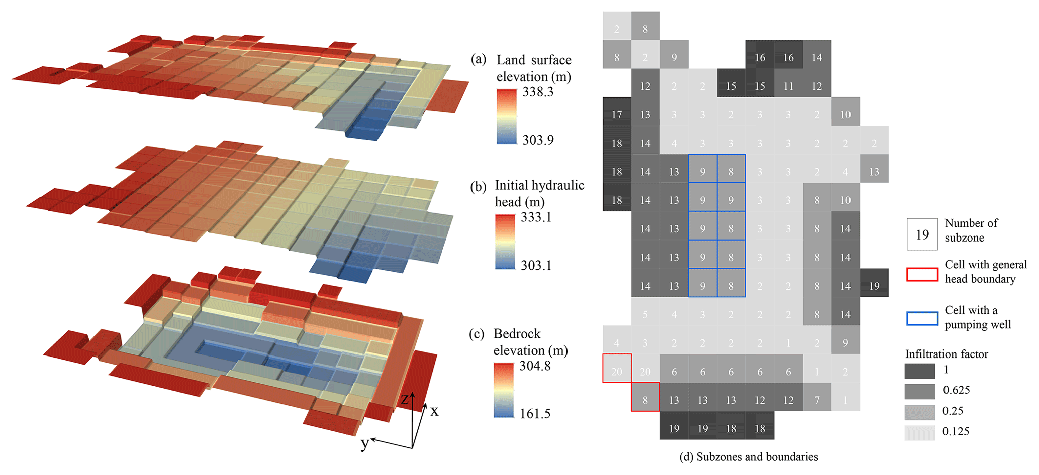
Figure 6Input of the synthetic regional problem including (a) land surface elevation, (b) initial head, (c) bedrock elevation of the aquifer, and (d) the subzones and boundaries.
4.1 Reducing the complexity of a feedback coupling system
The numerical difficulty in a coupled unsaturated–saturated flow system originates from the nonlinearity of the soil-water models, heterogeneity of the parameters, and the variability of the hydrologic stresses (Krabbenhøft, 2007; Zha et al., 2017). In our work, the overall complexity of an iteratively coupled quasi-3-D model could be lowered by (1) taking full advantage of the h- and θ-form REs to reduce the nonlinearity in the soil-water models and (2) smoothing the variability in the exchanged interfacial messages.
Two scenarios in case 1 were selected to address the first point. Sudden infiltration into a dry sandy soil and the rapidly altering atmospheric upper boundaries were tested to illustrate the importance of applying a switching-form RE for lowering the nonlinearity in the soil-water models. To evaluate the benefits brought by a switching-form RE, the numerical stability was first considered, as shown in Fig. 7. The coupled model in our work was tested with h-form and switching-form REs. Compared with the HYDRUS-1D model (also based on an h-form RE), the switching-form method was numerically more robust, i.e., with larger minimal time-step sizes (Δtmin) and a lower computational cost, where a minimal time-step size 10−3 days was stable for convergence. Notably at the beginning of the sudden infiltration into a dry sandy soil, in Fig. 7a, the Δtmin for a switching method was 10−3 days, even at early infiltration times, while for the h-form methods, including HYDRUS-1D and the coupled h-form method, Δtmin was constrained to 10−8 days before reaching a painstaking convergence. In Fig. 8, the soil-water content solution by the coupled switching-form method and the HYDRUS-1D method (taken as the truth) were compared at depths of 0, 50, and 200 cm. The RMSEs of the soil moisture solutions (θ) at three different depths are respectively 0.0189, 0.0032, and 0.0013. To finish the calculation, the coupled switching-form RE method took 17 s, while it took 41 s for the HYDRUS code. When solving the same problem, the matrix equation set was solved 4903 times with the switching scheme, while it was solved 10 925 times for the HYDRUS-1D code. The switched governing equations contribute toward cutting the computational cost by half for problems with rapidly changing upper boundary conditions. Here, the threshold for choosing an appropriate form of RE was non-sensitive to the numerical efficiency. A wide range of Secritϵ [0.3, 0.9] was suggested according to substantial trial-and-error tests.
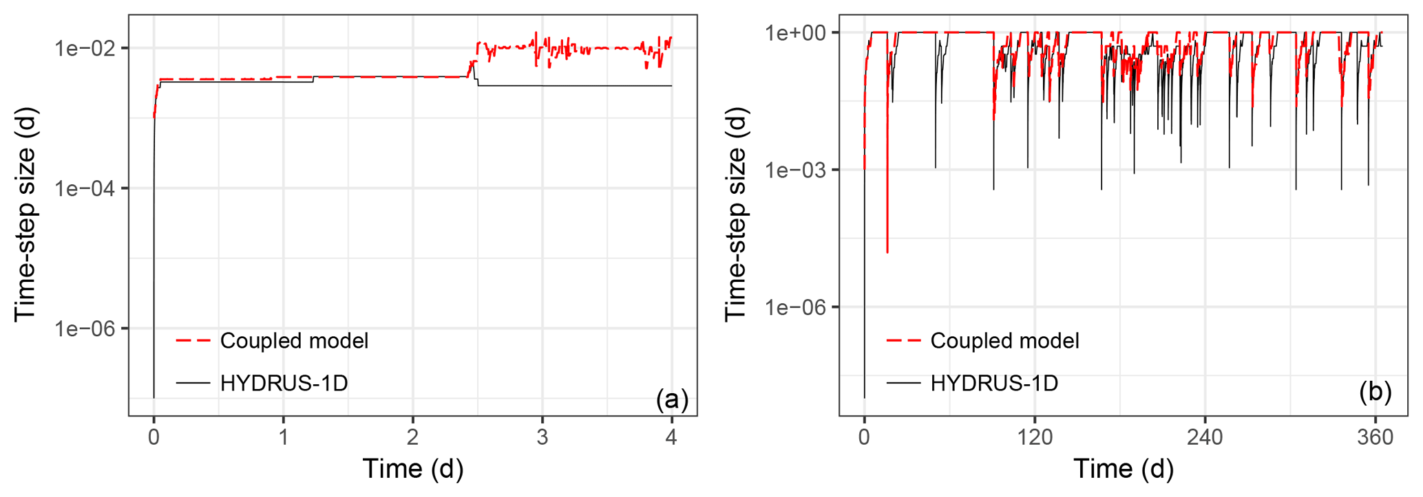
Figure 7The time-step sizes through the simulation of (a) sudden infiltration into a dry sandy soil column and (b) rapidly changing atmospheric upper boundary conditions with a layered soil column.
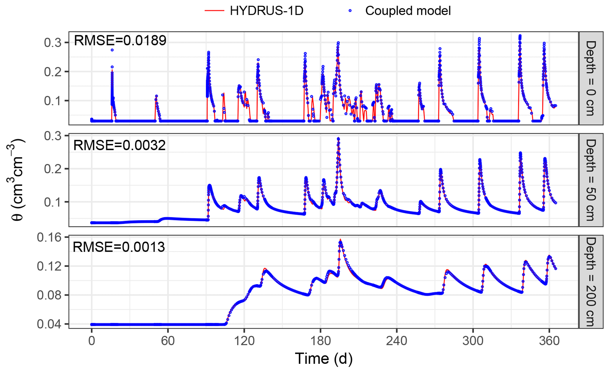
Figure 8Comparison of soil moisture content at z=0, 50, and 200 cm for the layered soil column with rapidly changing upper boundary conditions (scenario 2, case 1). Taking the HYDRUS-1D solution as the truth, RMSEs of solution of the developed model are provided at different soil depths.
Reducing the complexity of a coupling system can also be attained by smoothing the exchanged information in space and time. As suggested by Stoppelenburg et al. (2005), a time-varying specific yield calculated by the small-scale soil-water models, in Eq. (12), introduced significant variability to the large-scale groundwater model, thus caused extra iterations. A large-scale reduced the nonlinearity of the storage term in the groundwater equation. In case 1, using an of 0.1–0.2 in the groundwater model produced best numerical stability for the sandy soil with dramatically uprising water table. With a large-scale , the nonlinearity introduced by the small-scale soil-water models could be quickly smoothed, as shown in Eq. (12).
4.2 Multi-scale water balance analysis
The traditional non-iterative feedback coupling methods cannot maintain sound mass balance near the phreatic surface, especially for problems with drastic flow interactions.
One reason is that, to launch a new step of a sub-model at either side of the phreatic interface, the non-iterative feedback methods usually employed a predicted interfacial boundary without correction, which inevitably introduced coupling errors. In traditional non-iterative methods (Seo et al., 2007; Xu et al., 2012), such shortcomings could be alleviated by refining the macro-time-step size (ΔT). However, the Dirichlet head predicted for the soil columns with a stepwise extension method (see Fig. 2a) was easy to implement but tended to suffer from significant coupling error. In this work, we proposed a linear extrapolation method for the lower boundary head prediction for the soil-water models (see Eq. A2). Here, we used niter to indicate the maximal number of feedback iteration. Compared with a traditional stepwise method, the solution obtained by a linear method, either iteratively (with niter =3) or non-iteratively (niter =0), was easier for approaching the truth (see Fig. 9). Even with refined macro-time-step sizes (ΔT from 0.2 to 0.005 days), the stepwise method made a thorough effort to minimize the coupling errors. Notably, three feedback iterations (niter =3) were sufficient for reducing the coupling error significantly. Such a one-dimensional case with constant upper boundary flux, avoiding interference from lateral fluxes, illustrated the importance of a temporal scale-matching analysis for coupling the soil-water and groundwater models.
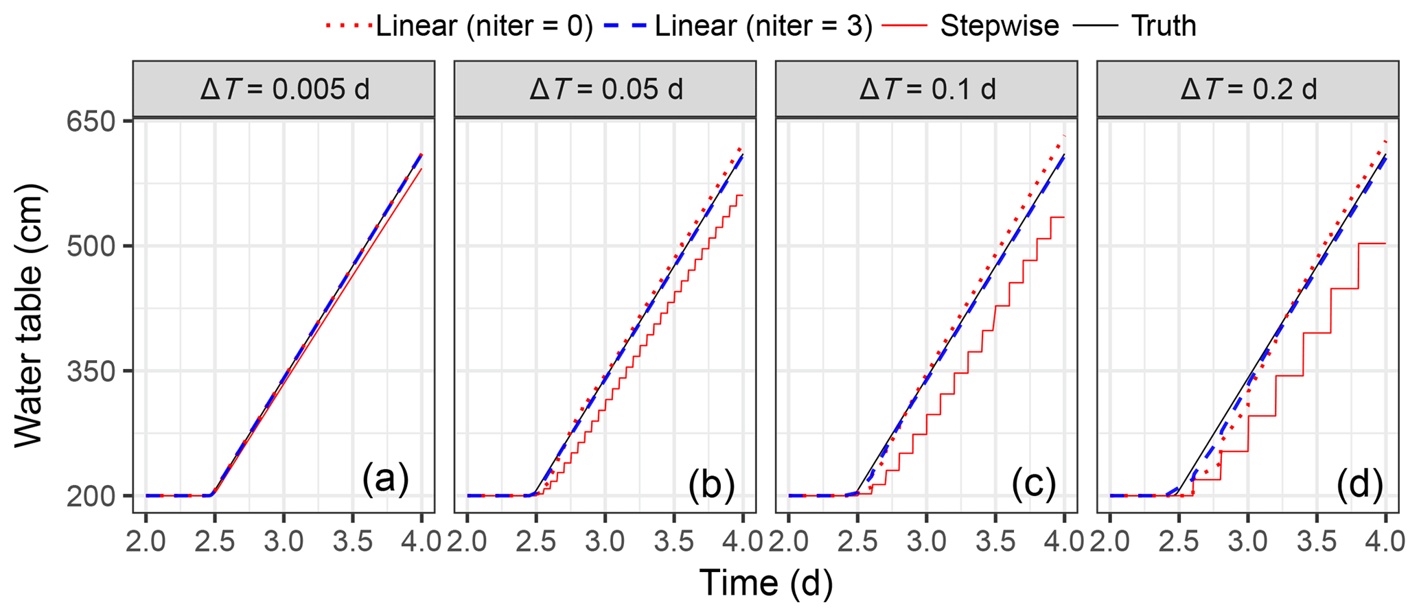
Figure 9Water table changing with time for different macro-time-step sizes (ΔT=0.005, 0.05, 0.1, and 0.2 days), in scenario 1, case 1. The HYDRUS-1D solution is taken as the truth. Compared with the stepwise extended method (Seo et al., 2007), the coupling error is significantly reduced by a linear prediction.
The other factor contributing to the coupling errors in the traditional method lies in neglecting the saturated lateral flux between adjacent soil columns (Seo et al., 2007; Stoppelenburg et al., 2005; Xu et al., 2012). In practical applications, the fluxes in and out of the saturated parts of the soil columns differ, which adds to the complexity of the coupling scheme. Although a strict water balance equation is established (Shen and Phanikumar, 2010), the concern centers on the spatial scale-mismatching problem. That is, when the coarse-grid groundwater flow solutions are converted into the vertically distributed fine-scale source and sink terms for the soil columns, an extra downscaling approach is needed to ensure their accuracy. Here we carried out a multi-scale water balance analysis above the phreatic surface. The fine-scale saturated lateral flows were thus excluded from Eq. (10). The benefits of the moving-boundary approach can be seen in case 2, which produces significant saturated lateral flux. We carried out a comparative analysis against the traditional stationary-boundary methods (Seo et al., 2007; Xu et al., 2012). The 2-D solution of VSF was taken as the truth. Figure 10 presents the effectiveness of the moving-boundary method. Five stationary soil columns with three different lengths (L=1000, 500, and 300 cm) were compared with an adaptively moving soil column within the iterative feedback coupling scheme. The cross-sectional RMSE of the phreatic surface and the head at the bottom layer (z=0) are presented in Fig. 10a and b. The soil columns with bottom nodes fixed deeply into the aquifer, instead of moving with the phreatic surface, introduced large coupling errors. This was caused by the nontrivial saturated lateral fluxes between the adjacent soil columns. With a traditional stationary-boundary method, such problems can be alleviated by avoiding large saturated lateral fluxes between the soil columns. However, for some spatiotemporally varying local events in a regional aquifer (e.g., pumping or flooding irrigation), such problems increased the burden for subzone partitioning. A moving-boundary method, instead, was numerically more efficient in minimizing the size of the matrix equation and reducing the coupling errors.
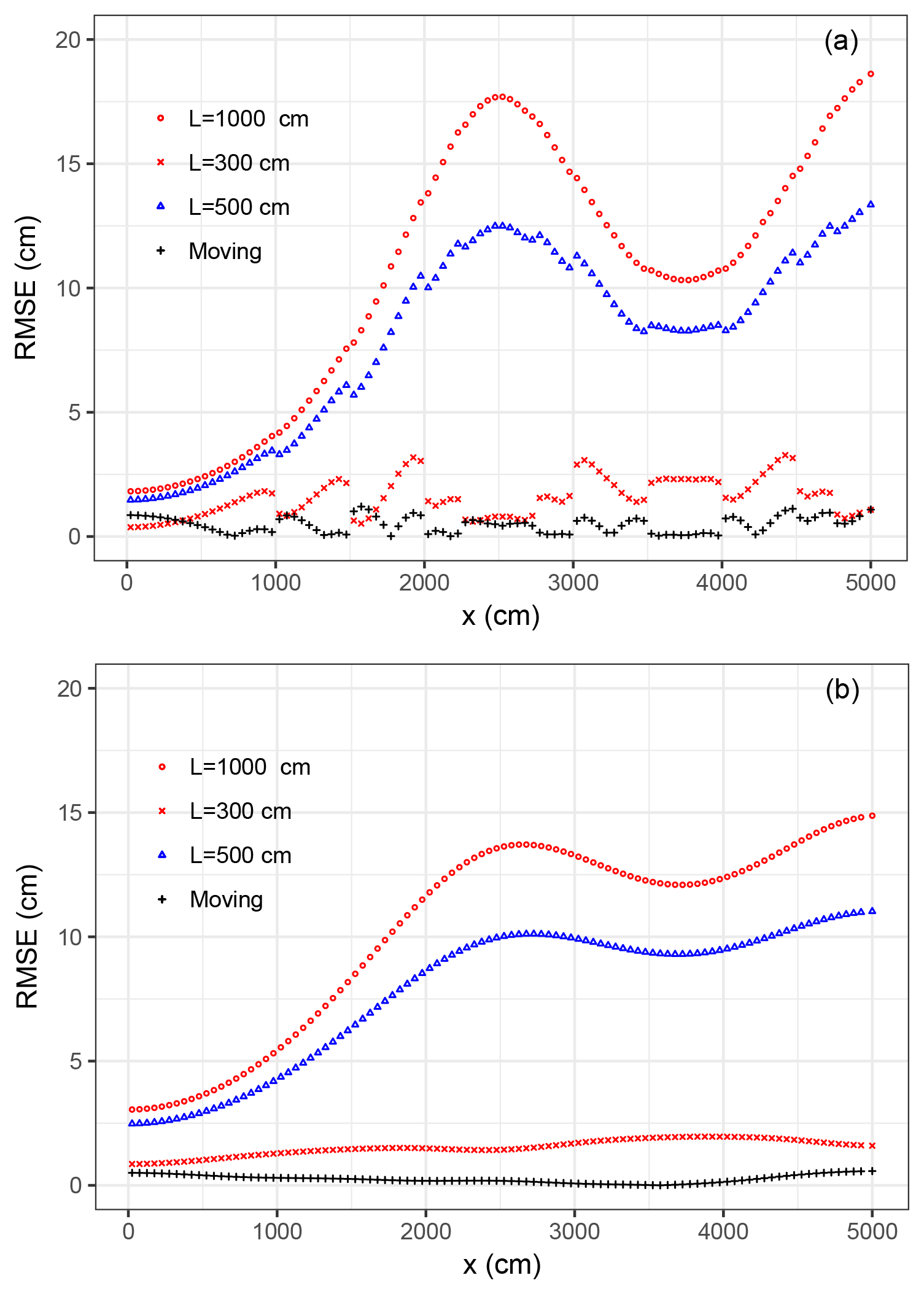
Figure 10Comparison of RMSE of (a) the phreatic surface and (b) the head solution (at z=0) between the moving-boundary and the stationary-boundary methods. Three different lengths of the stationary soil columns, L=1000, 500, and 300 cm, are considered.
4.3 Regulating the feedback iterations
In coupling two complicated modeling systems, a common agreement has been reached that; feedback coupling, either iteratively (Markstrom et al., 2008; Mehl and Hill, 2013; Stoppelenburg et al., 2005; Xie et al., 2012) or non-iteratively (Seo et al., 2007; Shen and Phanikumar, 2010; Xu et al., 2012), is numerically more rigorous than the one-way coupling scheme. The main difference between the above two methods lies in the ability to conserve mass within a single step for back-and-forth information exchange. In an iterative method, the head and/or flux boundaries are iteratively exchanged. There is a cost–benefit tradeoff for obtaining higher numerical efficiency.
During the late stages of the recharge in scenario 1 of case 1, the groundwater table rises quickly, which increases the burden on the coupling scheme. In our work, feedback iteration was conducted to eliminate the coupling error within the back-and-forth boundary exchange. To investigate how the feedback iteration influences the numerical accuracy as well as computational cost, solutions were compared with different closure criteria, instead of different maximal numbers of feedback iterations. For this purpose, scenario 1 in case 1 is tested with a range of closure criteria indicated by closure =0.001, 0.01, 0.1, 1, 5, and 20. Specifically, closure =20 (i.e., εH=20 cm) is too large to regulate any feedback iteration and is thus replaced by “non-iterative”. The εF, indicating the closure of the Neumann boundary feedback iteration, is usually related to the phreatic Darcian flux. To avoid its impact on the discussion below, we assume that , which means no regulation from the flux boundary exchange. Due to less dynamic in the groundwater sub-model, the empirical relaxation factors were both set by 1.0 to have a straightforward update of the interfacial boundaries, i.e., zt and Ftop.
When the wetting front approached the phreatic surface (at t=2.4 days), the number of feedback iterations increased dramatically (see Fig. 11a). This was caused by the intensive rise of the water table within each macro-time step ΔT. The head and/or flux interfacial boundaries were thus not easy to approximate the truth. With several attempts to exchange the head and/or flux boundaries, the head solution was effectively drawn towards the truth, (see Fig. 11b). With closure < 2, i.e., εH < 2 cm, the coupling errors were significantly reduced (see Fig. 11c). The cost–benefit curve, which was quantified by the number of feedback iteration and the RMSE, was indicative of problems at larger scales and higher dimensionalities.
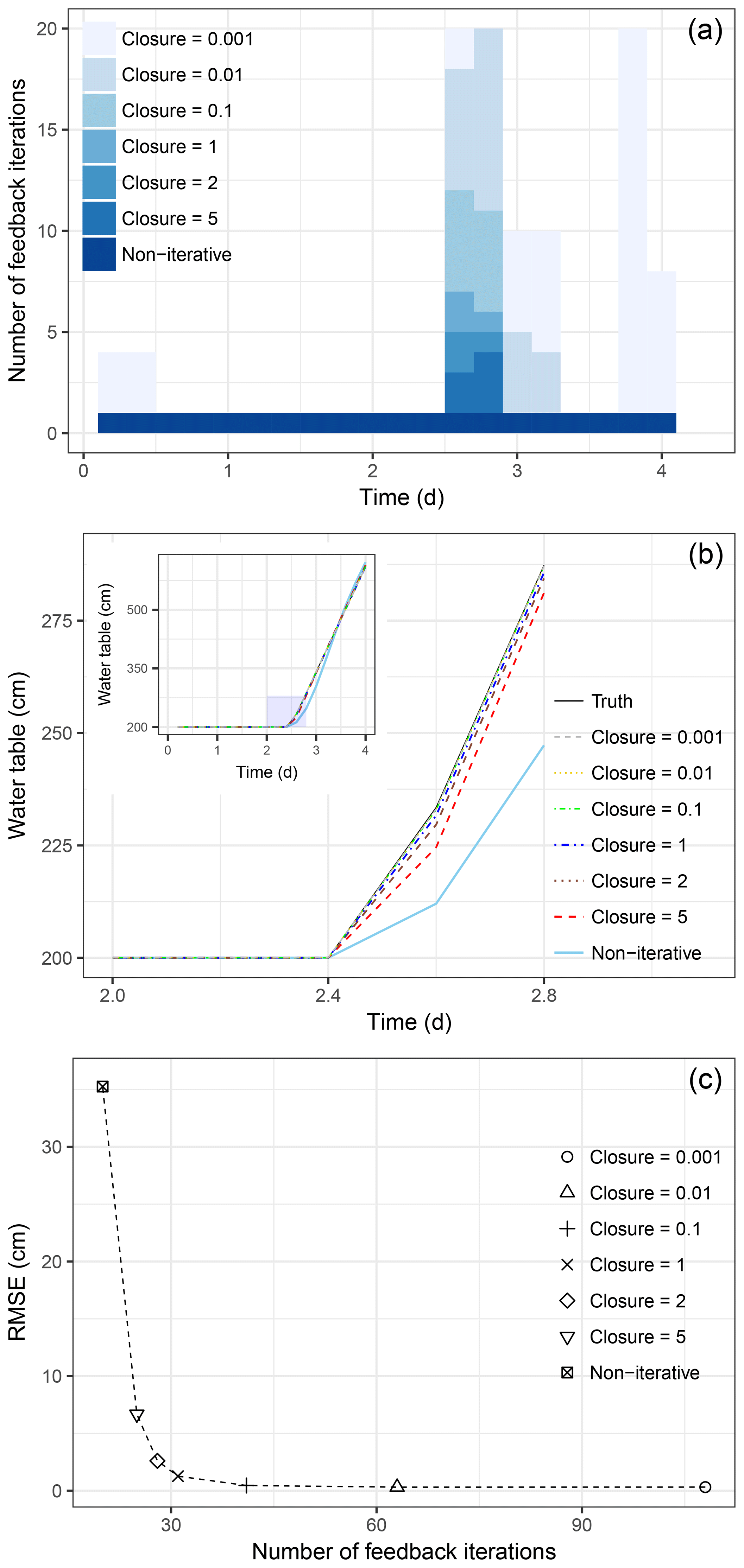
Figure 11(a) The number of feedback iterations and (b) phreatic surface solutions changing with different closure criteria. In the legend, “closure =0.001” means that εH=0.001 cm is used to regulate the feedback iteration. The HYDRUS-1D solution is taken as truth. Tested in scenario 1, case 1.
4.4 Parsimonious decision-making
The feedback coupling schemes, either iteratively or non-iteratively, increase the degree of freedom of the users to manage the sub-models with different governing equations, numerical algorithms, and the heterogeneities in parameters and variabilities in hydrologic stresses. For practical purposes, a significant concern is how to efficiently handle the complicated and scale-disparate systems.
For problems with rapid changes in groundwater flows, as in case 2, the hydraulic gradient at the phreatic surface was large. Using a single soil column for such a complex situation introduced significant coupling errors at the water table, (see Fig. 12a). Although more subzones portioned means higher accuracy for the coupling method, five or more soil columns were adequate enough in approaching the truth. Furthermore, for the saturated nodes deep in the aquifer, such differences in coupling errors were of minor influence (see Fig. 12b).
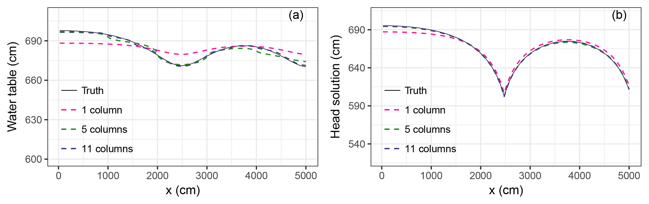
Figure 12Comparison of (a) water table and (b) head solution (at z=0) that are changing by the number of soil columns. Solutions obtained with a moving-boundary method in case 2.
In case 3, a simple pumped and irrigated region was simulated with different numbers of soil columns. A range of tests with total numbers of 16, 12, 9, 5, and 3 soil columns were carried out to obtain a cost–benefit curve, shown in Fig. 13c. When partitioning the vadose zone into more than 12 soil columns, there was a slight reduction in solution errors (RMSE) and a significant increase in the computational cost caused by solving more 1-D soil-water models. Although parallelled computation could further reduce the numerical cost, representing the vadose zone with three sequentially calculated soil-water models achieved acceptable accuracy, as presented in Fig. 13a and b. The computational cost for obtaining the fully 3-D solution with VSF was 15.561 s, which was more than 11 times larger than an iterative feedback coupling method with soil-water models sequentially solved. Problems in more complicated real-world situations can thus be simplified to achieve higher numerical efficiency.
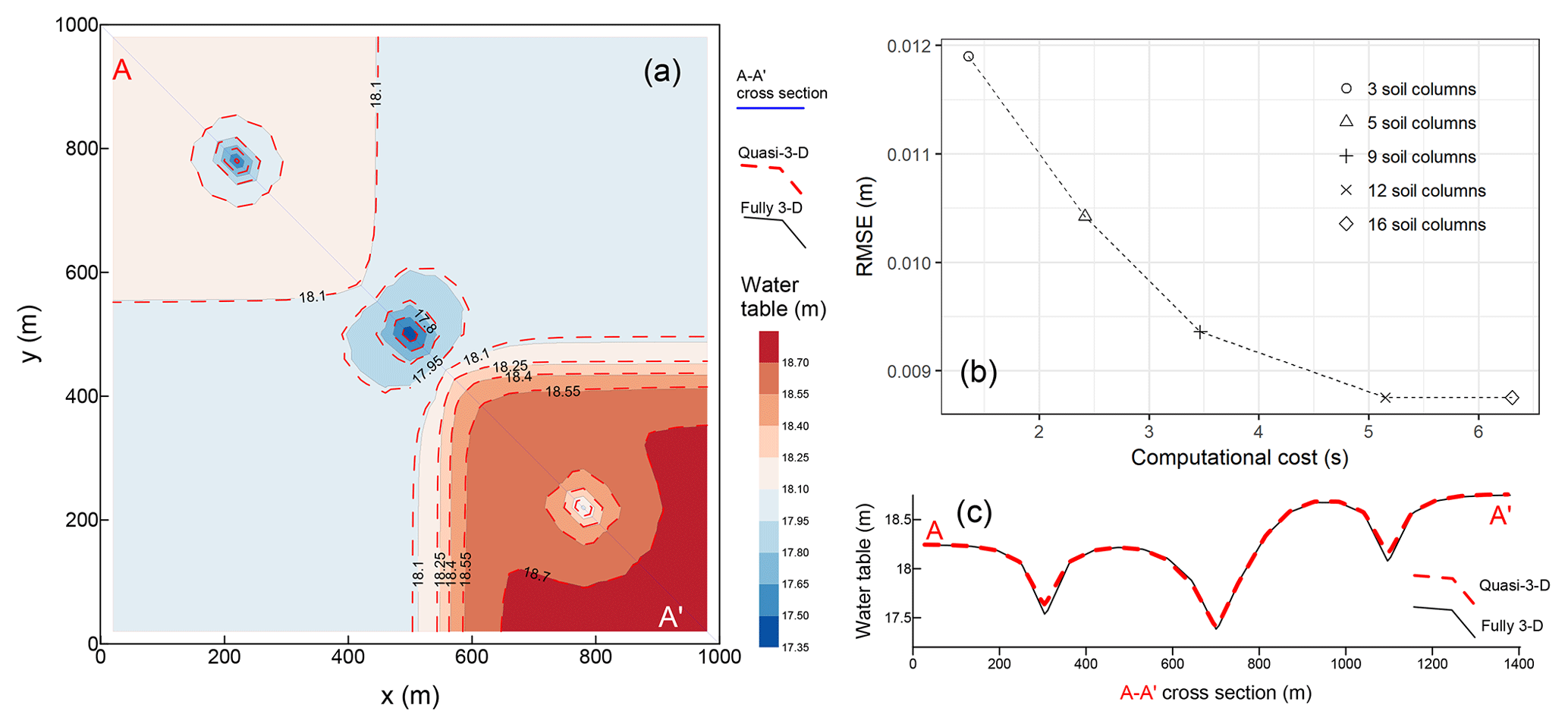
Figure 13(a) Comparison of contours of the phreatic surface solution obtained with the fully 3-D and quasi-3-D methods. (b) Comparison of the phreatic surface at A–A' cross section; (c) computational cost and RMSE changing by the number of total soil columns.
4.5 Regional application
Prudic et al.'s problem was originally designed to validate a streamflow routing package (Prudic et al., 2004). Stressed by soil surface infiltration, pumping wells, and the general head boundary, the synthetic case was used to evaluate several unsaturated flow packages for MODFLOW (Twarakavi et al., 2008). Based on their studies, in case 4, we compared the developed iterative feedback coupling method with HPM. The hydraulic conductivity, as well as its heterogeneity, was forced to be consistent within the saturated and unsaturated zones, which is different from the case in Twarakavi et al. (2008). Figure 14a gives the contours for the final phreatic head solutions, indicating a good match of the phreatic surface with the HYDRUS package. Figure 14b–e present the absolute head difference of the method developed here and the HYDRUS package at the end of stress periods 3, 6, 9, and 12. The dark color blocks indicated the largest difference in the head solution. According to Fig. 6d, the saturated grid cells controlled by the soil columns of no. 3, no. 9, no. 10, no. 15, and no. 19 were suffering from the largest deviation, although with the same horizontal partitioning of the unsaturated zone. The strict iteratively two-way coupling contributes to such an accuracy improvement.
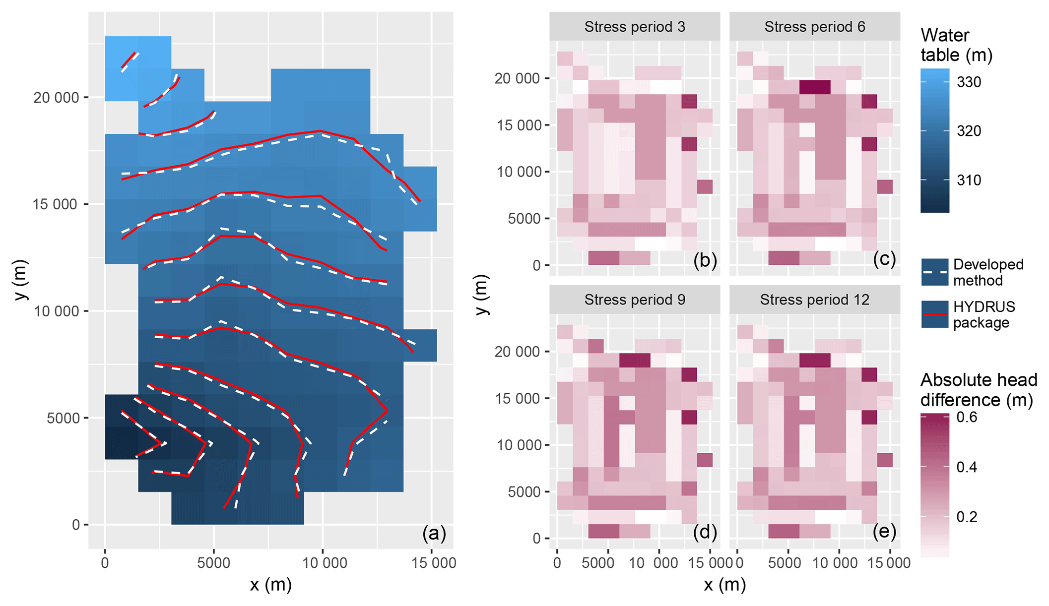
Figure 14(a) Comparison of elevation of the water table calculated by the HYDRUS package for MODFLOW (Seo et al., 2007) and the developed method (t=365 days). (b) The absolute head difference of the phreatic head solution by the method developed here and HYDRUS package at the end of stress periods 3, 6, 9, and 12 (case 4).
For unsaturated–saturated flow situations, the vadose zone flow is important. Figure 15 presents the water content profiles at subzones 1, 3, 5, 7, and 9 as examples. The solution obtained from the developed model matched well with the original HPM solution. For practical purposes, the manually controlled stress periods for the unsaturated sub-models are no longer constrained. In our method, the soil-water models run at disparate numerical scales, which makes it possible to handle daily or hourly observed information rather than a stress period lasting 2 or more days in traditional coupled models.

Figure 15Comparison of water content profiles obtained from the HYDRUS package for MODFLOW (Seo et al., 2007) and the developed iterative feedback coupling method. Subzones 1, 3, 5, 7, and 9 are shown as an example. (t=365 days in case 4).
Fully 3-D numerical models are available but are numerically expensive for simulating the regional unsaturated–saturated flow. The quasi-3-D method presented here, in contrast, with horizontally disconnected adjacent unsaturated nodes, significantly reduces the dimensionality and complexity of the problem. Such a simplification brings about computational cost saving and flexibility for better manipulation of the sub-models. However, the nonlinearity in the soil-water retention curve, as well as the variability in realistic boundary stresses of the vadose and saturated zones, usually results in the scale-mismatching problems when attempting numerical coupling. In this work, the soil-water and groundwater models were coupled with an iterative feedback (two-way) coupling scheme. Three concerns about the multi-scale water balance at the phreatic interface are addressed using a range of numerical cases in multiple dimensionalities. We conclude with the following:
-
A new HYDRUS package for MODFLOW was developed by switching the θ and h forms of Richards' equation (RE) at each numerical node. The switching RE circumvents the disadvantages of the h- and θ-form REs to achieve higher numerical stability and computational efficiency. The one-dimensional switching RE was employed to simulate the rapid infiltration into a dry sandy soil, and the swiftly altering atmospheric upper boundaries in a layered soil column. Compared with the h-form RE, the switching RE used a 105 times larger minimal time-step size (Δtmin) and conserved mass better. Lowering the nonlinearity of soil-water models with this switching scheme was promising for coupling complex flow modeling systems at the regional scale.
-
Stringent multi-scale water balance analysis at the water table was conducted to handle scale-mismatching problems and to smooth the information delivered back and forth across the interface. In our work, the errors originating from inadequate phreatic boundary predictions were reduced firstly by a linear extrapolation method and then by an iterative feedback. Compared with the traditional stepwise extension method, the linear extrapolation significantly reduced the coupling errors caused by scale mismatching. For problems with severe soil-water and groundwater interactions, the coupling errors were significantly reduced by using an iterative feedback coupling scheme. The multi-scale water balance analysis mathematically maintained numerical stabilities in the sub-models at disparate scales.
-
When a moving phreatic boundary was assigned to the soil columns during the phreatic water balance analysis, it avoided the coupling errors originating from the saturated lateral fluxes. In practical applications for regional problems, the fluxes into and out of the saturated parts of the soil columns differed, which added to the complexity and phreatic water balance error of the coupling scheme. With a moving Dirichlet lower boundary, the saturated regions of the soil-water models were removed. The coupling error was significantly reduced for problems with major groundwater flow. Extra cost saving was achieved by minimizing the matrix sizes of the soil-water models.
Future investigation will focus on regional solute transport modeling based on the developed coupling scheme. Surface flow models, as well as the crop models, which appear to be less nonlinear than the subsurface models, will be coupled in an object-oriented modeling system. The RS- and GIS-based data class can then be used to handle more complicated large-scale problems.
All the data and codes used in this study can be requested by email to the corresponding author Yuanyuan Zha at zhayuan87@gmail.com.
A1 The moving Dirichlet lower boundary
The bottom node of a soil column is adaptively located at the phreatic surface, which makes it an area-averaged moving Dirichlet boundary:
where zt(T) (L) is the elevation of the water table; Π is the control domain of a soil column; H(T) (L) is potentiometric head solution, as well as the elevation of the phreatic surface, which is obtained by solving the groundwater model; and s is the horizontal area.
To simulate the multi-scale flow process within a macro-time step , the lower boundary head of a soil column is temporally predicted either by stepwise extension of zt(TJ) (Seo et al., 2007; Shen and Phanikumar, 2010; Xu et al., 2012) or by linear extrapolation from zt(TJ+1) and zt(TJ). In Fig. 2a, the stepwise extension method () potentially causes large deviation from the truth. In our study, the linear extrapolation is resorted to for reducing the coupling errors and accelerating the convergence of the feedback iteration. The small-scale lower boundary head at time t () is given by
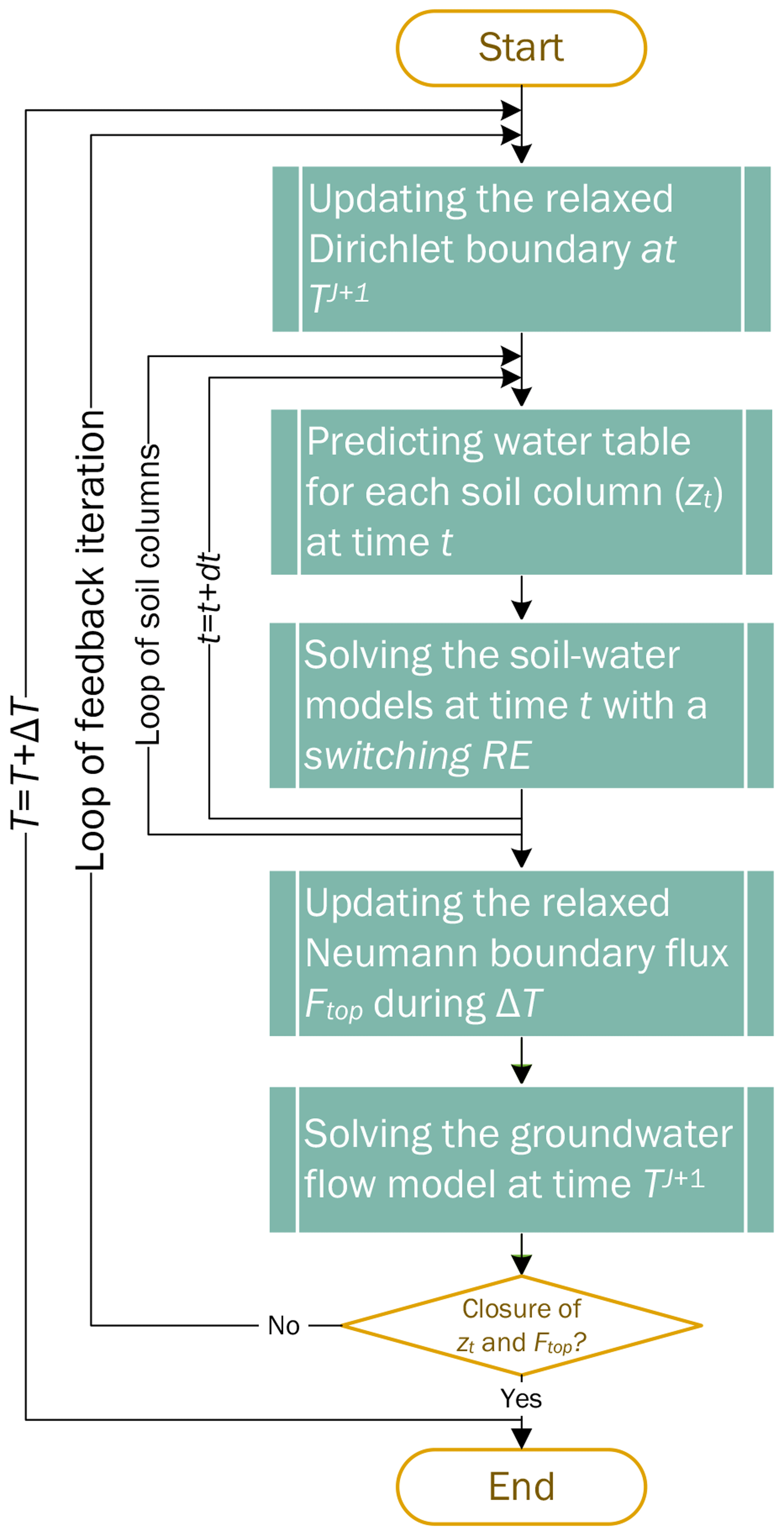
Figure A1Flowchart of the relaxed iterative feedback coupling scheme. The relaxation is conducted at the interfacial Dirichlet–Neumann boundaries during the feedback iterations (except for the time TJ).
A2 The Neumann upper boundary
The moving Dirichlet boundary introduces the need for water balance of a moving balancing domain above the water table (see Fig. 2b), which is bounded by a specific elevation above the phreatic surface, zs (L), and the dynamically changing phreatic surface, zt(t) (L).
Assuming that the activated top layer in a three-dimensional groundwater model is conceptualized into a phreatic aquifer, the governing equation for this layer is given by
where (L) is the thickness of the phreatic layer, which is numerically defined as the layer below the vadose zone, ; z0 is the bottom elevation of the top phreatic layer, z0 ≪zs; Ftop (L T−1) is the groundwater recharge into the activated top layer of the phreatic aquifer, ; and Fbase is the leakage into an underlying numerical layer, (positive downward, like Ftop). The long-term regional-scale parameter indicating the water yield caused by the fluctuation of the water table (Nachabe, 2002), , (–), is calculated by
where Vw (L3) is the amount of water release caused by fluctuation of the phreatic surface (ΔH (L)), and A (L2) is the area of interest.
A3 The relaxed iterative feedback coupling
The relaxed feedback iteration method (Funaro et al., 1988; Mehl and Hill, 2013) is used to improve the convergence of head and/or flux at the phreatic surface (see Fig. A1). The Dirichlet lower boundary head for the soil columns, zt, as well as the Neumann upper boundary flux for the phreatic surface, Ftop, are updated within each iterative step (niter):
where superscripts old (or new) indicate the previous (or newly calculated) head and/or flux boundaries at the coupling interface, and λh and λf are the empirical relaxation factors for head and/or flux boundaries respectively. Their values are suggested to be within . The iteration ends when agreements are reached at
where εH (L) and εF (L T−1) are residuals for the feedback iteration of the interfacial head and flux.
JZ, YZ, and JY developed the new package for soil-water movement based on a switching Richards' equation; JZ and YZ developed the coupling methods for efficiently joining the sub-models. JZ, YZ, JY, and LS made non-negligible efforts in preparing the paper.
The authors declare that they have no conflict of interest.
This work was funded by the Chinese National Natural Science Foundation
(no. 51479143 and 51609173). The authors would thank Ian White and
Wenzhi Zeng for their laborious revisions and helpful suggestions for the
paper as well as the editorial team for the HESS Journal.
Edited by: Bob Su
Reviewed by: two anonymous
referees
Bailey, R. T., Morway, E. D., Niswonger, R. G., and Gates, T. K.: Modeling variably saturated multispecies reactive groundwater solute transport with MODFLOW-UZF and RT3D, Groundwater, 51, 752–761, https://doi.org/10.1111/j.1745-6584.2012.01009.x, 2013.
Celia, M. A., Bouloutas, E. T., and Zarba, R. L.: A general mass-conservative numerical solution for the unsaturated flow equation, Water Resour. Res., 26, 1483–1496, https://doi.org/10.1029/WR026i007p01483, 1990.
Crevoisier, D., Chanzy, A., and Voltz, M.: Evaluation of the Ross fast solution of Richards' equation in unfavourable conditions for standard finite element methods, Adv. Water Resour., 32, 936–947, https://doi.org/10.1016/j.advwatres.2009.03.008, 2009.
Dettmann, U. and Bechtold, M.: One-dimensional expression to calculate specific yield for shallow groundwater systems with microrelief, Hydrol. Process., 30, 334–340, https://doi.org/10.1002/hyp.10637, 2016.
Diersch, H. J. G. and Perrochet, P.: On the primary variable switching technique for simulating unsaturated-saturated flows, Adv. Water Resour., 23, 271–301, https://doi.org/10.1016/S0309-1708(98)00057-8, 1999.
Downer, C. W. and Ogden, F. L.: Appropriate vertical discretization of Richards' equation for two-dimensional watershed-scale modelling, Hydrol. Process., 18, 1–22, https://doi.org/10.1002/hyp.1306, 2004.
Edwards, M. G.: Elimination of Adaptive Grid Interface Errors in the Discrete Cell Centered Pressure Equation, J. Comput. Phys., 126, 356–372, https://doi.org/10.1006/jcph.1996.0143, 1996.
Forsyth, P. A., Wu, Y. S., and Pruess, K.: Robust numerical methods for saturated-unsaturated flow with dry initial conditions in heterogeneous media, Adv. Water Resour., 18, 25–38, https://doi.org/10.1016/0309-1708(95)00020-J, 1995.
Funaro, D., Quarteroni, A., and Zanolli, P.: An iterative procedure with interface relaxation for domain decomposition methods, Siam J. Numer. Anal., 25, 1213–1236, https://doi.org/10.1137/0725069, 1988.
Grygoruk, M., Batelaan, O., Mirosław-Świltek, D., Szatyłowicz, J., and Okruszko, T.: Evapotranspiration of bush encroachments on a temperate mire meadow – A nonlinear function of landscape composition and groundwater flow, Ecol. Eng., 73, 598–609, https://doi.org/10.1016/j.ecoleng.2014.09.041, 2014.
Gunduz, O. and Aral, M. M.: River networks and groundwater flow: A simultaneous solution of a coupled system, J. Hydrol., 301, 216–234, https://doi.org/10.1016/j.jhydrol.2004.06.034, 2005.
Hao, X., Zhang, R., and Kravchenko, A.: A mass-conservative switching method for simulating saturated-unsaturated flow, J. Hydrol., 301, 254–265, https://doi.org/10.1016/j.jhydrol.2005.01.019, 2005.
Harbaugh, A. W.: MODFLOW-2005, the U.S. Geological Survey modular ground-water model: The ground-water flow process, US Department of the Interior, US Geological Survey Reston, VA, USA, 2005.
Hills, R. G., Porro, I., Hudson, D. B., and Wierenga, P. J.: Modeling one-dimensional infiltration into very dry soils: 1. Model development and evaluation, Water Resour. Res., 25, 1259–1269, https://doi.org/10.1029/WR025i006p01259, 1989.
Krabbenhøft, K.: An alternative to primary variable switching in saturated-unsaturated flow computations, Adv. Water Resour., 30, 483–492, https://doi.org/10.1016/j.advwatres.2006.04.009, 2007.
Kumar, M., Duffy, C. J., and Salvage, K. M.: A Second-Order Accurate, Finite Volume-Based, Integrated Hydrologic Modeling (FIHM) Framework for Simulation of Surface and Subsurface Flow, Vadose Zone J., 8, 873–890, https://doi.org/10.2136/vzj2009.0014, 2009.
Kuznetsov, M., Yakirevich, A., Pachepsky, Y. A., Sorek, S., and Weisbrod, N.: Quasi 3D modeling of water flow in vadose zone and groundwater, J. Hydrol., 450–451, 140–149, https://doi.org/10.1016/j.jhydrol.2012.05.025, 2012.
Langevin, C. D., Hughes, J. D., Banta, E. R., Provost, A. M., Niswonger, R. G., and Panday, S.: MODFLOW 6 Groundwater Flow (GWF) Model Beta version 0.9.03, U.S. Geol. Surv. Provisional Softw. Release, https://doi.org/10.5066/F76Q1VQV, 2017.
Leake, S. A. and Claar, D. V: Procedures and computer programs for telescopic mesh refinement using MODFLOW, Citeseer, available at: http://az.water.usgs.gov/MODTMR/tmr.html (last access: 29 January 2019), 1999.
Lin, L., Yang, J.-Z., Zhang, B., and Zhu, Y.: A simplified numerical model of 3-D groundwater and solute transport at large scale area, J. Hydrodyn. Ser. B, 22, 319–328, https://doi.org/10.1016/S1001-6058(09)60061-5, 2010.
Liu, Z., Zha, Y., Yang, W., Kuo, Y., and Yang, J.: Large-Scale Modeling of Unsaturated Flow by a Stochastic Perturbation Approach, Vadose Zone J., 15, https://doi.org/10.2136/vzj2015.07.0103, 2016.
Markstrom, S. L., Niswonger, R. G., Regan, R. S., Prudic, D. E., and Barlow, P. M.: GSFLOW – Coupled Ground-Water and Surface-Water Flow Model Based on the Integration of the Precipitation-Runoff Modeling System (PRMS) and the Modular Ground-Water Flow Model (MODFLOW-2005), Geological Survey (US), available at: https://pubs.usgs.gov/tm/tm6d1/ (last access: 29 January 2019), 2008.
Maxwell, R. M. and Miller, N. L.: Development of a coupled land surface and groundwater model, J. Hydrometeorol., 6, 233–247, https://doi.org/10.1175/JHM422.1, 2005.
McDonald, M. G. and Harbaugh, A. W.: A modular three-dimensional finite-difference ground-water flow model, available at: http://pubs.er.usgs.gov/publication/twri06A1 (last access: 29 January 2019), 1988.
Mehl, S. and Hill, M. C.: Three-dimensional local grid refinement for block-centered finite-difference groundwater models using iteratively coupled shared nodes: a new method of interpolation and analysis of errors, Adv. Water Resour., 27, 899–912, https://doi.org/10.1016/j.advwatres.2004.06.004, 2004.
Mehl, S. and Hill, M. C.: MODFLOW–LGR – Documentation of ghost node local grid refinement (LGR2) for multiple areas and the boundary flow and head (BFH2) package, 2013th ed., available at: https://pubs.usgs.gov/tm/6a44 (last access: 29 January 2019), 2013.
Miller, C. T., Williams, G. A., Kelley, C. T., and Tocci, M. D.: Robust solution of Richards' equation for nonuniform porous media, Water Resour. Res., 34, 2599–2610, https://doi.org/10.1029/98WR01673, 1998.
Miller, C. T., Abhishek, C., and Farthing, M. W.: A spatially and temporally adaptive solution of Richards' equation, Adv. Water Resour., 29, 525–545, https://doi.org/10.1016/j.advwatres.2005.06.008, 2006.
Nachabe, M. H.: Analytical expressions for transient specific yield and shallow water table drainage, Water Resour. Res., 38, 11-1–11-7, https://doi.org/10.1029/2001WR001071, 2002.
Niswonger, R. G., Prudic, D. E., and Regan, S. R.: Documentation of the Unsaturated-Zone Flow (UZF1) Package for Modeling Unsaturated Flow Between the Land Surface and the Water Table with MODFLOW-2005, US Department of the Interior, US Geological Survey, available at: https://pubs.er.usgs.gov/publication/tm6A19 (last access: 29 January 2019), 2006.
Niswonger, R. G., Panday, S., and Ibaraki, M.: MODFLOW-NWT, a Newton formulation for MODFLOW-2005, US Geol. Surv. Tech. Methods, 6, A37, available from: https://pubs.usgs.gov/tm/tm6a37 (last access: 29 January 2019), 2011.
Panday, S. and Huyakorn, P. S.: A fully coupled physically-based spatially-distributed model for evaluating surface/subsurface flow, Adv. Water Resour., 27, 361–382, https://doi.org/10.1016/j.advwatres.2004.02.016, 2004.
Panday, S., Langevin, C. D., Niswonger, R. G., Ibaraki, M., and Hughes, J. D.: MODFLOW–USG version 1: An unstructured grid version of MODFLOW for simulating groundwater flow and tightly coupled processes using a control volume finite-difference formulation, US Geological Survey, https://doi.org/10.3133/tm6A45, 2013.
Paulus, R., Dewals, B. J., Erpicum, S., Pirotton, M., and Archambeau, P.: Innovative modelling of 3D unsaturated flow in porous media by coupling independent models for vertical and lateral flows, J. Comput. Appl. Math., 246, 38–51, https://doi.org/10.1016/j.cam.2012.07.032, 2013.
Prudic, D. E., Konikow, L. F., and Banta, E. R.: A New Streamflow-Routing (SFR1) Package to Simulate Stream-Aquifer Interaction with MODFLOW-2000, available at: http://pubs.er.usgs.gov/publication/ofr20041042 (last access: 29 January 2019), 2004.
Richards, L. A.: Capillary conduction of liquids through porous mediums, J. Appl. Phys., 1, 318–333, https://doi.org/10.1063/1.1745010, 1931.
Rybak, I., Magiera, J., Helmig, R., and Rohde, C.: Multirate time integration for coupled saturated/unsaturated porous medium and free flow systems, Comput. Geosci., 19, 299–309, https://doi.org/10.1007/s10596-015-9469-8, 2015.
Seo, H. S., Šimůnek, J., and Poeter, E. P.: Documentation of the HYDRUS Package for MODFLOW-2000, the U.S. Geological Survey Modular Ground-Water Model, GWMI 2007-01, Int. Ground Water Modeling Center, Colorado School of Mines, Golden, CO, 96 pp., 2007.
Shen, C. and Phanikumar, M. S.: A process-based, distributed hydrologic model based on a large-scale method for surface-subsurface coupling, Adv. Water Resour., 33, 1524–1541, https://doi.org/10.1016/j.advwatres.2010.09.002, 2010.
Šimůnek, J., Sejna, M., Saito, H., Sakai, M., and van Genuchten, M. T.: The HYDRUS-1D software package for simulating the one-dimensional movement of water, heat, and multiple solutes in variably-saturated media, Version 4.08, 2009.
Šimůnek, J., Van Genuchten, M. T., and Šejna, M.: Recent Developments and Applications of the HYDRUS Computer Software Packages, Vadose Zone J., 15, https://doi.org/10.2136/vzj2016.04.0033, 2016.
Stoppelenburg, F. J., Kovar, K., Pastoors, M. J. H., and Tiktak, A.: Modelling the interactions between transient saturated and unsaturated groundwater flow. Off-line coupling of LGM and SWAP, RIVM Rep., 500026001, 70, 2005.
Thoms, R. B., Johnson, R. L., and Healy, R. W.: User's guide to the variably saturated flow (VSF) process to MODFLOW, available at: http://pubs.er.usgs.gov/publication/tm6A18 (last access: 29 January 2019), 2006.
Twarakavi, N. K. C., Šimůnek, J., and Seo, S.: Evaluating Interactions between Groundwater and Vadose Zone Using the HYDRUS-Based Flow Package for MODFLOW, Vadose Zone J., 7, 757–768, https://doi.org/10.2136/vzj2007.0082, 2008.
van Dam, J. C., Groenendijk, P., Hendriks, R. F. A., and Kroes, J. G.: Advances of Modeling Water Flow in Variably Saturated Soils with SWAP, Vadose Zone J., 7, 640–653, https://doi.org/10.2136/vzj2007.0060, 2008.
van Genuchten, M. T.: A Closed-form Equation for Predicting the Hydraulic Conductivity of Unsaturated Soils, Soil Sci. Soc. Am. J., 44, 892–898, https://doi.org/10.2136/sssaj1980.03615995004400050002x, 1980.
Vogel, H.-J. and Ippisch, O.: Estimation of a Critical Spatial Discretization Limit for Solving Richards' Equation at Large Scales, Vadose Zone J., 7, 112–114, https://doi.org/10.2136/vzj2006.0182, 2008.
Warrick, A. W.: Numerical approximations of darcian flow through unsaturated soil, Water Resour. Res., 27, 1215–1222, https://doi.org/10.1029/91WR00093, 1991.
Xie, Z., Di, Z., Luo, Z., and Ma, Q.: A Quasi-Three-Dimensional Variably Saturated Groundwater Flow Model for Climate Modeling, J. Hydrometeorol., 13, 27–46, https://doi.org/10.1175/JHM-D-10-05019.1, 2012.
Xu, X., Huang, G., Zhan, H., Qu, Z., and Huang, Q.: Integration of SWAP and MODFLOW-2000 for modeling groundwater dynamics in shallow water table areas, J. Hydrol., 412–413, 170–181, https://doi.org/10.1016/j.jhydrol.2011.07.002, 2012.
Yakirevich, A., Borisov, V., and Sorek, S.: A quasi three-dimensional model for flow and transport in unsaturated and saturated zones: 1. Implementation of the quasi two-dimensional case, Adv. Water Resour., 21, 679–689, https://doi.org/10.1016/S0309-1708(97)00031-6, 1998.
Zadeh, K. S.: A mass-conservative switching algorithm for modeling fluid flow in variably saturated porous media, J. Comput. Phys, 230, 664–679, https://doi.org/10.1016/j.jcp.2010.10.011, 2011.
Zeng, J., Zha, Y., Zhang, Y., Shi, L., Zhu, Y., and Yang, J.: On the sub-model errors of a generalized one-way coupling scheme for linking models at different scales, Adv. Water Resour., 109, 69–83, https://doi.org/10.1016/j.advwatres.2017.09.005, 2017.
Zeng, J., Zha, Y., and Yang, J.: Switching the Richards' equation for modeling soil water movement under unfavorable conditions, J. Hydrol., 563, 942–949, https://doi.org/10.1016/j.jhydrol.2018.06.069, 2018.
Zha, Y., Shi, L., Ye, M., and Yang, J.: A generalized Ross method for two- and three-dimensional variably saturated flow, Adv. Water Resour., 54, 67–77, https://doi.org/10.1016/j.advwatres.2013.01.002, 2013a.
Zha, Y., Yang, J., Shi, L., and Song, X.: Simulating One-Dimensional Unsaturated Flow in Heterogeneous Soils with Water Content-Based Richards Equation, Vadose Zone J., 12, https://doi.org/10.2136/vzj2012.0109, 2013b.
Zha, Y., Yang, J., Yin, L., Zhang, Y., Zeng, W., and Shi, L.: A modified Picard iteration scheme for overcoming numerical difficulties of simulating infiltration into dry soil, J. Hydrol., 551, 56–69, https://doi.org/10.1016/j.jhydrol.2017.05.053, 2017.
Zhu, Y., Shi, L., Lin, L., Yang, J., and Ye, M.: A fully coupled numerical modeling for regional unsaturated-saturated water flow, J. Hydrol., 475, 188–203, https://doi.org/10.1016/j.jhydrol.2012.09.048, 2012.