the Creative Commons Attribution 4.0 License.
the Creative Commons Attribution 4.0 License.
 | 28 Nov 2019
Spatio-temporal relevance and controls of preferential flow at the landscape scale
Dominic Demand
Theresa Blume
Markus Weiler
The spatial and temporal controls of preferential flow (PF) during infiltration are still not fully understood. As soil moisture sensor networks allow us to capture infiltration responses in high temporal and spatial resolution, our study is based on a large-scale sensor network with 135 soil moisture profiles distributed across a complex catchment. The experimental design covers three major geological regions (slate, marl, sandstone) and two land covers (forest, grassland) in Luxembourg. We analyzed the responses of up to 353 rainfall events for each of the 135 soil moisture profiles. Non-sequential responses (NSRs) within the soil moisture depth profiles were taken as one indication of bypass flow. For sequential responses maximum porewater velocities (vmax) were determined from the observations and compared with velocity estimates of capillary flow. A measured vmax higher than the capillary prediction was taken as a further indication of PF. While PF was identified as a common process during infiltration, it was also temporally and spatially highly variable. We found a strong dependence of PF on the initial soil water content and the maximum rainfall intensity. Whereas a high rainfall intensity increased PF (NSR, vmax) as expected, most geologies and land covers showed the highest PF under dry initial conditions. Hence, we identified a strong seasonality of both NSR and vmax dependent on land cover, revealing a lower occurrence of PF during spring and increased occurrence during summer and early autumn, probably due to water repellency. We observed the highest fraction of NSR in forests on clay-rich soils (slate, marl). vmax ranged from 6 to 80 640 cm d−1 with a median of 120 cm d−1 across all events and soil moisture profiles. The soils in the marl geology had the highest flow velocities, independent of land cover, especially between 30 and 50 cm depth, where the clay content increased. This demonstrates the danger of treating especially clay soils in the vadose zone as a low-conductive substrate, as the development of soil structure can dominate over the matrix property of the texture alone. This confirms that clay content and land cover strongly influence infiltration and reinforce PF, but seasonal dynamics and flow initiation also have an important impact on PF.
- Article
(4156 KB) - Full-text XML
-
Supplement
(792 KB) - BibTeX
- EndNote


Preferential flow (PF) in soils describes different flow processes with higher flow velocities than soil matrix flow and heterogeneous flow patterns (Hendrickx and Flury, 2001). Many studies have shown that PF is ubiquitous (Jarvis, 2007) and that “PF is the norm and not the exception” (Weiler, 2017). PF can affect water distribution in soil (Ritsema et al., 1996), groundwater recharge (Ireson and Butler, 2011), root water uptake (Schwärzel et al., 2009) and solute transport (Larsbo et al., 2014). Since the early work of Beven and Germann (1982), the importance of PF pathways such as macropores (created by roots, earthworms), fissures or cracks has been widely recognized. Most studies focusing on different PF processes, such as fingered flow (Selker et al., 1992), macropore flow (Weiler and Naef, 2003) or funnel flow (Kung, 1990), were carried out at the point or plot scale (spatial scale smaller than a few meters). Since PF increases the range of flow velocities in the vadose zone by orders of magnitudes (Nimmo, 2007), it is essential to include this process when modeling water and solute transport in soil. Given its importance, many models now account for PF processes (see Gerke, 2006; Köhne et al., 2009; Steinbrich et al., 2016), but defining meaningful parameter sets for these models is challenging (Abbaspour et al., 2004; Arora et al., 2011; Cheng et al., 2017). Furthermore, Reck et al. (2018) showed that macropore networks and related parameters such as macropore distance and diameter are not constant over time. The problem of spatial and temporal variability of PF is also reflected in the updated paper about PF research by Beven and Germann (2013). They stated that some fundamental questions are still not solved. One of the central questions raised by Beven and Germann (2013) is “When does water flow through macropores in the soil?”. We know about the importance of PF, but knowledge about the spatial and temporal properties affecting the distribution of PF across the landscape is still lacking (Lin et al., 2006; Wiekenkamp et al., 2016).
Many methods have been developed in the last decades to study and quantify PF in soils (see, e.g., Allaire et al., 2009). These methods include using X-ray tomography at the pore to soil core scale (Larsbo et al., 2014; Naveed et al., 2016), the analysis of (dye) tracers and breakthrough curves at the soil core to hillslope scale (Anderson et al., 2009; Flury et al., 1994; Koestel et al., 2013; Zehe and Flühler, 2001) or using geophysical methods at the plot to hillslope scale (Angermann et al., 2017; Oberdörster et al., 2010). Another way to identify the potential for PF are measurements that can be related to the number and volume of macropores or cracks. Watson and Luxmoore (1986) used a tension infiltrometer to calculate the amount of infiltration that is caused by pores of a specific equivalent pore size, a method that has been frequently used (e.g., Buttle and McDonald, 2000). Stewart et al. (2016a, b) measured soil crack structure and volume and used this information to model soil water infiltration. Nevertheless, most methods lack either spatial or temporal resolution to quantify the frequency and properties of PF simultaneously for larger areas (∼ km2) and longer timescales (∼ years).
An alternative approach to study PF during infiltration are soil moisture measurements at high temporal resolution (∼ minutes). While soil moisture sensors only measure at the point or profile scale, they can be deployed widely throughout the landscape (Zehe et al., 2014). Soil moisture sensors can be installed at different depths and are minimally invasive (Hardie et al., 2013). So far, soil moisture sensors were used to detect PF by either using the measured response velocities after a rainfall event (Blume et al., 2009; Eguchi and Hasegawa, 2008; Germann and Hensel, 2006; Hardie et al., 2013; Kim et al., 2007) or for analyzing the sequence of their response with depth (Graham and Lin, 2011; Lin and Zhou, 2008; Liu and Lin, 2015; Wiekenkamp et al., 2016). Using these methods most studies found a relationship with precipitation characteristics (Liu and Lin, 2015; Wiekenkamp et al., 2016) or initial soil moisture (Blume et al., 2009; Hardie et al., 2013; Liu and Lin, 2015; Wiekenkamp et al., 2016).
Even though some of the studies described above show differences in PF occurrence between soils or landscape properties, most of them do not rigorously compare contrasting landscape units at the larger scale. Zhao et al. (2012) tested out-of-sequence responses of the soil moisture sensors as an indication of PF for two contrasting land covers and found much higher occurrence of PF in the forest sites compared to a cropland. However, since both sites also had different soils, it could not clearly be attributed to land cover. Most field experiments studying the effect of soil texture and land cover on soil water flow measured infiltration characteristics or hydraulic conductivities of soil cores (Bormann and Klaassen, 2008; Gonzalez-Sosa et al., 2010; Jarvis et al., 2013; Zimmermann et al., 2006). In general, higher infiltration rates and hydraulic conductivities were observed at sites with natural vegetation or forests. These higher infiltration rates were often attributed to the presence of macropores, but not connected to the dynamics of PF occurrence under natural field conditions. Studies linking the spatial and temporal PF occurrence in high resolution and comparing contrasting landscapes under natural initial and boundary conditions are still scarce.
A correct estimation of PF occurrence is important for hydrological predictions (e.g., modeling) and can improve water resource management. Therefore, the main aim of this study is to identify and compare the temporal dynamic of PF occurrence by using profiles of soil moisture sensors in different large-scale spatial units that could potentially be used as representative units for catchment modeling. Since it can be expected that rainfall intensity and soil moisture have a strong influence on the initialization of PF (Beven and Germann, 1982), we will mainly focus on the temporal controls of initial soil moisture and rainfall. More specifically, we attempt to answer the following questions. Does PF occurrence increase with rainfall intensity since higher intensity leads more frequently to an exceedance of matrix infiltration capacity? Does PF occur more often under wet conditions since the infiltration capacity is lower? How is the temporal PF dynamic influenced by spatial factors like geology/soil type and land cover?
2.1 Study sites
To test our research question we analyzed a dataset of 405 soil moisture sensors at 45 sites distributed across a complex landscape (varying geology and land cover) but under similar climatic conditions. The monitoring network is located in the Attert catchment in the Grand Duchy of Luxembourg. The climate is temperate semi-oceanic with a mean annual rainfall of 845 mm (Pfister et al., 2006), mean monthly temperatures between 0 ∘C (January) and 17 ∘C (July) and only very few days per year with snow coverage (Wrede et al., 2015). Elevation ranges between 265 and 480 m a.s.l. and the catchment covers three major geologies (Colbach and Maquil, 2003). The northwestern part of the catchment is located at the southern edge of the Ardennes and the geology here is dominated by Devonian Slate bedrock covered by periglacial slope deposits mixed with eolian loess (Juilleret et al., 2011; Moragues-Quiroga et al., 2017). The southern part of the catchment is dominated by sedimentary rocks of the Paris Basin (Wrede et al., 2015) with Jurassic Luxembourg Sandstone at the southern catchment border and Triassic Sandy Marls in the central part of the catchment (Fig. 1). The slate region has agriculturally used plateaus between steep forested slopes (∼15–25∘). The sandstone hillslopes are mostly forested with grasslands only present on the footslopes (Juilleret et al., 2012; Martínez-Carreras et al., 2012). The land cover in the Luxembourgian part of the marl region is mainly characterized by agricultural sites (30 %) and grasslands (41 %, mainly pasture) with gentle slopes (∼3∘).
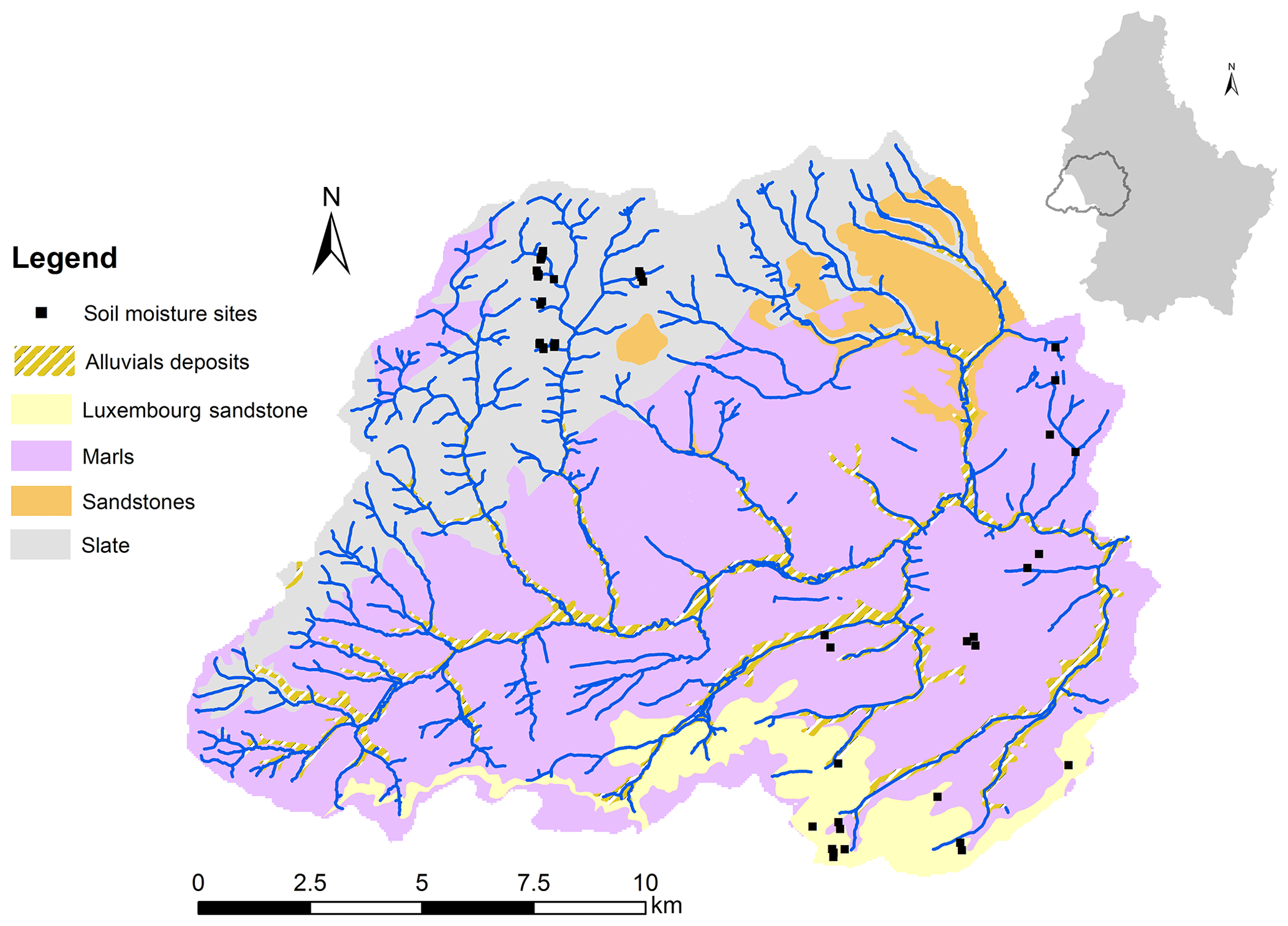
Figure 1Map of the Attert catchment in Luxembourg with the three main geologies and the locations of the 45 soil moisture monitoring sites.
Table 1Site information of the six defined landscape units. Additional textural information can be found in the Supplement (Table S1). Texture denoted with ∗ was estimated with a field test by feel. Date format is mm/yyyy.
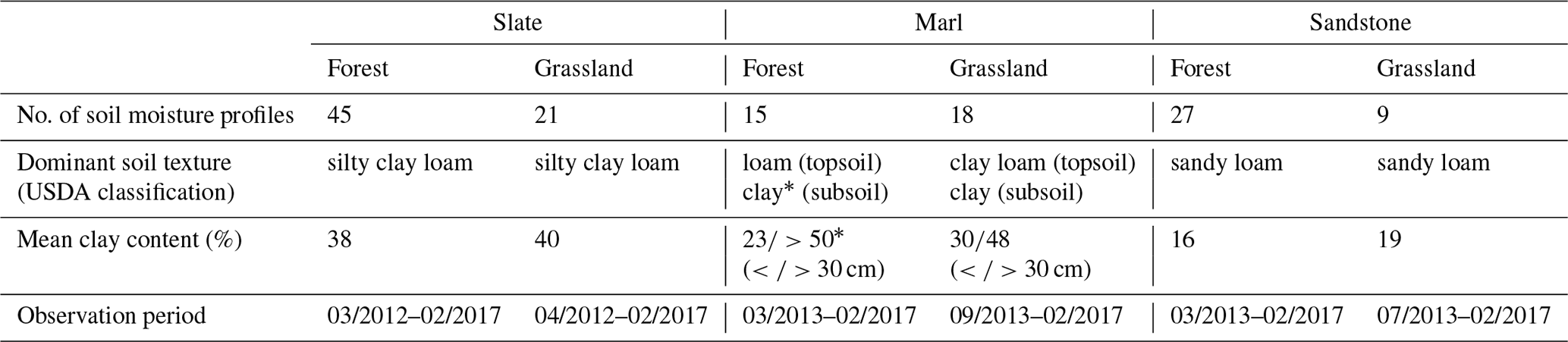
Soil types in the slate geology are Haplic Cambisols (Ruptic, Endosketelic, Siltic) (IUSS Working Group WRB, 2006) with a main texture of silty clay loam (Table 1). Texture was determined by sedimentation analysis following DIN ISO 11277 (2002) from randomly distributed samples taken mostly in the upper 30 cm. Coarse particle fraction (>2 mm) was much higher than in the other geologies and is estimated between 10 % and up to 50 % volume fraction in the Bw horizon and increases with depth. Layers of weathered rock (C horizon) are found usually below 50 cm. Weathered slate rocks are mostly embedded slope parallel due to solifluction of the soil layers during the last ice age (Juilleret et al., 2011). In the Luxembourg Sandstone, Colluvic Arenosols dominate in the valley bottom and Podzols (IUSS Working Group WRB, 2006) with a sandy loam texture on the slopes and plateaus. The depth to the unweathered bedrock is more than 2 m (Sprenger et al., 2015) with banded Bt horizons deeper than 1 m. The soils of the marl geology have a more diverse texture (Wrede et al., 2015) but are often showing a clay rich layer (>50 % clay) starting between 20 and 50 cm depth. Therefore, Stagnosols (IUSS Working Group WRB, 2006) are very common in this region. Sandy horizons can be found as well, whereas topsoils mostly exhibit a loamy texture (Table 1). The soils show high macroporosity documented by the excavation of horizontal soil profiles and counting of pores >2 mm Ø.
The instrumentation at each site includes air temperature, groundwater table elevation and rainfall measurements and three soil moisture profiles separated by 5–20 m. A soil moisture profile consists of three volumetric soil moisture (θ) sensors at 10, 30 and 50 cm depth below the surface. In total 135 soil moisture profiles at 45 different sites were distributed across the catchment (Fig. 1). The time series used in this study start between March 2012 (first installed profiles) and October 2013 (last installed profiles) and end in February 2017 (Table 1). The soil moisture sensors (5TE capacitance sensors, METER Group Inc., USA) measured at 5 min temporal resolution. These sensors measure with a 70 MHz frequency and have a sample volume of around 300–715 mL (Cobos, 2015; Vaz et al., 2013), although other studies found smaller sampling volumes in wetter soils for other sensors of similar type (Blonquist et al., 2005). Due to sensor defects, 43 sensors were replaced with SMT100 (TRUEBNER GmbH, Neustadt, Germany) and 9 sensors with GS3 sensors (METER Environment, USA) in 2016. Sensors were installed horizontally with minimum disturbance from a 30 cm diameter hole drilled with a power auger. Each sensor was installed slightly shifted in the horizontal direction to the one above, to be unaffected by potential flow path changes by the sensor above. Furthermore, sensor cables were laid downwards in the hole first and led up on the opposite wall to prevent artificial PF along the cables leading to the sensors. In each of the three main geologies, the sensor sites were situated in two different land cover classes, forest and grassland. The selected forest sites were dominated by European beech (Fagus sylvatica) with occurrence of oak (Quercus robur, Quercus petraea) and common hornbeam (Carpinus betulus). Furthermore, rainfall was measured with one tipping bucket (Davis Instruments, USA, 0.2 mm resolution, collection area 214 cm2) at each grassland site and five randomly placed tipping buckets at each forest site to account, to at least some degree, for the spatial variability of throughfall. We defined six different landscape units distinguishing the three main geological formations and the two land covers (forest, grassland) to test our research questions. The number of soil moisture profiles for the different land cover and geological classes are summarized in Table 1. Additional information and specific site properties are shown in Appendix A.
2.2 Data analysis
2.2.1 Event classification
Rainfall events
A full workflow of the data analysis is depicted in Fig. 2 showing the number of excluded events due to different quality criteria. Rainfall (P) events were defined using the rainfall data with 5 min resolution individually for each site. For the forest sites the mean of all five tipping buckets for every 5 min time step was calculated to obtain average throughfall for each site. Forest tipping buckets that measured no rainfall over one hour were excluded (assuming they were clogged), when at least three other buckets observed rainfall during the same timeframe. If the rainfall data contained more than one missing value in a 2 h period, it was excluded from further analysis. Following the approach of Graham and Lin (2011) and Wiekenkamp et al. (2016), a rainfall event was defined as rainfall with a minimum amount of 1 mm. The end was defined as the last monitored response of a rain gauge followed by a specific time period without rain (te). The procedure of determining this time period is described below.
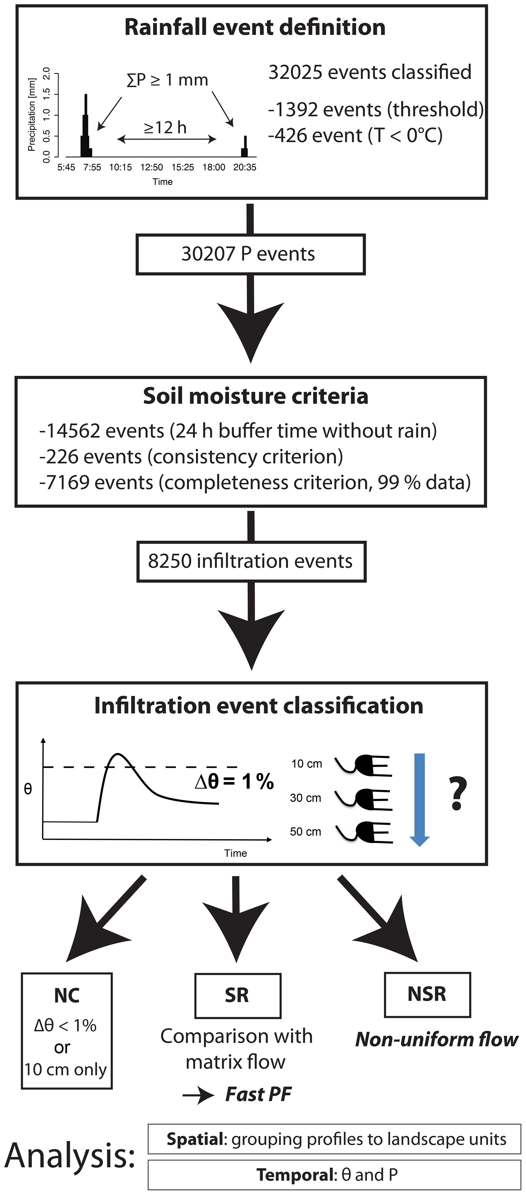
Figure 2Workflow for the estimation of spatial and temporal PF occurrence from soil moisture data with the number of included and excluded events. Event numbers refer to the sum of the events on a profile base (since this number is the resulting number of data points used for each analysis).
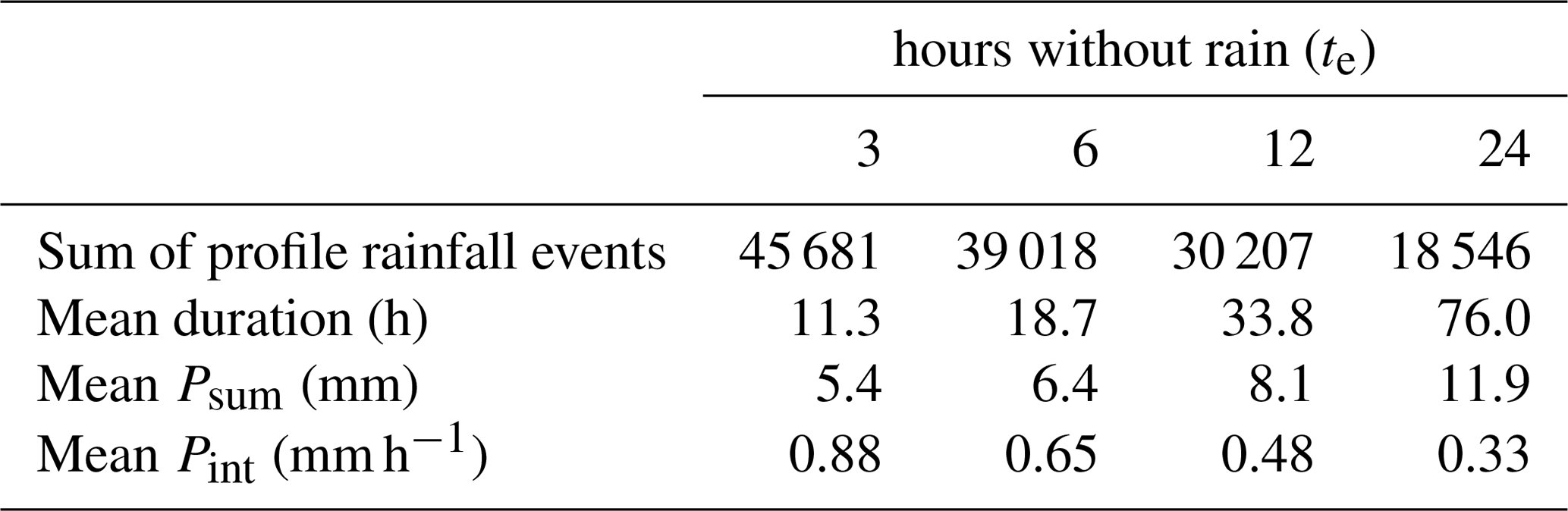
Dividing soil water dynamics into single events based on P input is always a trade-off: on the one hand, short rainfall events do not allow for a clear separation of the infiltration signals from different input pulses. On the other hand, long rainfall that is grouped into one event can result in too much information from several consecutive rain input pulses that are merged into one rainfall event. Hence, different rainfall regimes require different threshold values, i.e., hours without rainfall (te) for the identification of event endings. The sensitivity of te to the number of rainfall events and their characteristics in our case was investigated by testing different values of te: 3, 6, 12 and 24 consecutive hours without rain.
For each P event total rainfall amount (Psum), the maximum P intensity in a 5 min time step (Pmax) and the event average rainfall intensity of the entire event (Pint) was determined. Events that were not plausible were excluded by using a threshold method for event P amount (Psum>100 mm), average event intensity (Pint>15 mm h−1) and maximum P intensity in a 5 min time step ( mm h−1). These implausible events were observed to happen during the reconnecting of the loggers following a logger error (no power etc.) or clogging and release of the clogged water. To exclude snowfall or frozen soil conditions, events with a mean air temperature below 0 ∘C during the event were not included in the analysis. By applying the quality criteria for rainfall events using te=12 h, 1392 of 32 025 rain events (sum of profile rainfall events) were excluded because of the threshold criteria and 426 because the mean temperature was below 0 ∘C during the event.
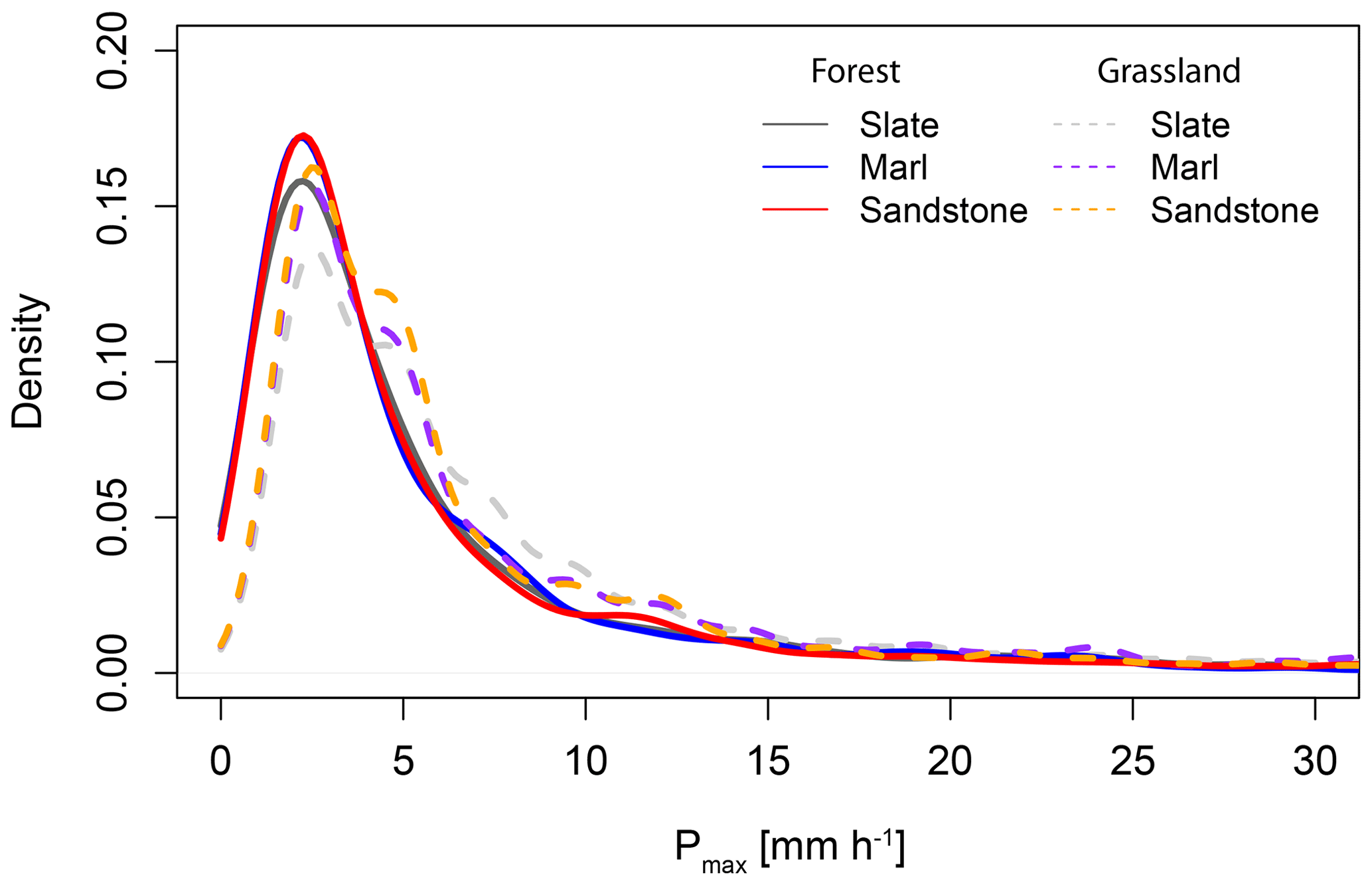
The rainfall event separation method is sensitive to the required number of consecutive hours without rain (te) between the events. Table 2 shows te values with the resulting number of events, mean event duration, rainfall amount (Psum) and event average rainfall intensity (Pint). Shorter te results in more events and decreasing mean event duration. Mean Pint is gradually decreasing with longer te due to longer event durations while mean Psum is increasing. We considered te=12 h to be sufficient to ensure event separation yielding an appropriate event length and to avoid possible superimposition of soil water flow signals from different input pulses. Therefore, the following analyses are performed with the event definition based on te=12 h. This results in total rainfall event numbers between 144 and 353 per profile. 54.2 % of all analyzed rainfall events had sums lower than 5 mm and 77.7 % lower than 10 mm. The distribution of rainfall intensities (Pint) shows that 69.2 % of all events had a Pint<0.4 mm h−1. The density distributions show slightly higher Pmax for grassland sites but no difference among the geologies (Fig. 3).
Table 2Rainfall event characteristics over all 135 profiles depending on minimum hours without rain (te) required between consecutive rainfall events.
Soil moisture and infiltration events
Signal spikes (strong increase in soil moisture within a 5 min time step and a decrease to the initial value) in the measured soil moisture time series were removed and data were visually checked for plausibility and long-term consistency. In addition, sensor readings were validated against those of the other sensors at the same depth for each site. No site-specific calibration of the soil moisture sensors was conducted and soil moisture values were obtained by the sensor-internal θ-permittivity relationship following Topp et al. (1980). For the 5TE sensors the manufacturer gives an absolute sensor accuracy of volumetric water content of ±3 vol % (DecagonDevices, 2016). For a relative change of 1 vol % a maximum sensor-to-sensor difference of ±0.25 vol % can be found in the very dry range (θ∼10 vol %) (Rosenbaum et al., 2010). Since Rosenbaum et al. (2011, 2012) showed that temperature effects on the sensors and on soil dielectric properties can cancel each other out, permittivity was not corrected for soil temperature. Furthermore, electrical conductivity effects of soil water on permittivity were neglected as bulk electrical conductivity was low (<0.1 dS m−1) for most profiles. Although some marl profiles show higher bulk electrical conductivities, results of soil water content change should not be affected since these profiles do not reveal fast bulk electrical conductivity fluctuations on the event scale.
For each defined rainfall event the soil moisture time series of all sensors in a profile was checked for their response. Infiltration events were defined as a θ increase of ≥1 vol % of at least one sensor in the soil profile. This threshold was chosen to avoid diurnal fluctuation, caused by, e.g., soil temperature, being classified as infiltration events (Graham and Lin, 2011; Wiekenkamp et al., 2016). If a soil moisture event was identified, the timing of the first response of every sensor was determined. The first response is defined as the point in time when the θ change is higher than the instrument noise (Lin and Zhou, 2008) that was found to be 0.4 vol % for the 5TE sensors (Rosenbaum et al., 2010; Wiekenkamp et al., 2016). Linear interpolation was used to calculate the time between two 5 min readings to increase the temporal resolution. The soil moisture response was tracked for up to 48 h after the end of a rainfall event or until the time a new rainfall event starts.
The chosen rainfall event separation based on te=12 h already avoids superimposition of consecutive rainfall input signals on the soil water content. However, to have clearly separated soil water flow events that are uninfluenced by a new rainfall event for at least 24 h, both consecutive infiltration events were excluded if the second rainfall event occurred within 24 h after the first rainfall event end. In the case of a response later than 24 h we assumed that the following infiltration event is likely to be triggered by the new rainfall event (Hardie et al., 2013). Only if more than 99 % of the data points for all profile sensors during an infiltration event were usable were they considered for further analysis (termed completeness criterion). Furthermore, infiltration events that showed an increase in soil moisture but were caused by an oscillating signal (not more than four different θ values during one event) were excluded (termed consistency criterion).
From the total of 30 207 rainfall events, 15 645 could be used for the analysis of the soil moisture, since they allowed for a clear separation of soil water flow by more than 24 h without a new rainfall input; 7395 of these events did not meet the quality criteria of completeness and consistency of the soil moisture time series; hence, 8250 infiltration events (the sum of soil moisture event observations at all 135 profiles) could be used for the analysis. Changing the completeness criterion from 99 % usable soil moisture data points during an event to, e.g., 95 % only slightly affects the number of infiltration events (e.g., 8353 events usable in the analysis). This is due to the fact that most exclusions result from long-term failure of one sensor of a profile that leads to a complete exclusion of the entire profile. A diagram showing the portion of active (all quality criteria met) profiles on a daily basis can be found in the Supplement (Fig. S1).
Various soil moisture and rainfall characteristics were determined for each event. Initial volumetric water content (θini) was defined as the water content before the rainfall event starts. Furthermore, change of θini to the peak water content (Δθmax) of every event and sensor response was calculated. We grouped soil moisture into dry and wet initial conditions using θ quartiles of each profile. Additionally, rainfall amounts and intensities were calculated for the time before the first soil moisture sensor response (Δθ=0.4 vol %) of any profile (rPsum, rPint, rPmax). This was done since our infiltration event classification described in the next section is partly based on the first sensor response and later rainfall input is not further influencing the classification.
2.2.2 Soil moisture sensor response by infiltration events
For all soil moisture profiles and rainfall events which met the described quality criteria, the sequence of the first sensor response was classified similarly to Liu and Lin (2015) into
- i.
not classifiable (NC): none of the sensors in the profile showed a response (≥1 vol %) or only a 10 cm sensor response was observed;
- ii.
non-sequential response (NSR): events where the first response did not progress in a sequence starting from the surface (e.g., the 30 cm sensor showed a response before the 10 cm sensor); and
- iii.
sequential response (SR): the sensors in the profile showed a response in the sequence from the uppermost sensor downwards (e.g., 10 to 30 to 50 cm or 10 to 30 cm).
The potential for using these different infiltration responses (SR, NSR) and related parameters as a proxy for PF is described in the following sections. All statistical analysis were performed using Dunn's rank sum test (Dinno, 2017).
Additionally, we estimated how often PF should have to be observed based on the classical assumption that rainfall intensity exceeded matrix infiltration capacity (Beven and Germann, 1982). We used matrix-saturated hydraulic conductivity (Kmat) as the minimum infiltration capacity and tested how often maximum 5 min rainfall intensity exceeded this threshold (; the measurements of Kmat are described at the end of the “Sequential response” section). Furthermore, comparison of maximum water content change during an event (Δθmax) between the infiltration response types can give information on PF processes by showing differing water content depth distributions and can help to estimate the relevance of the different flow processes in terms of transported water quantity.
Non-sequential response (NSR)
The NSR classification indicates non-uniform flow that can be a result of various PF processes (e.g., bypass flow); hence, it is taken as a proxy for PF. NSR could also be a result of subsurface lateral flow or groundwater rise before the vertically downward progressing wetting front reaches that depth (Lin and Zhou, 2008). But even in these cases, such responses describe water flow that shows either non-uniform flow or surroundings that infiltrate water faster than the profile. Both can be seen as an indication of PF. None of the profiles showed a permanent water table smaller than 50 cm below ground level; nevertheless, some profiles are influenced by groundwater fluctuations and are temporarily waterlogged at 50 cm, especially during winter. The length of the time series is adequate for detecting patterns of NSR, as Liu and Lin (2015) showed in their analysis that overall sensor response patterns show stable results using >3 years of soil moisture data. The occurrence frequency of NSR was analyzed with respect to initial soil moisture and rainfall characteristics for the landscape units. All NSR analyses were done with pre-response rainfall characteristics (rPsum, rPint, rPmax). Calculated portions of NSR for the landscape units, geologies or land covers for different rPmax, θini or months are always calculated as the sum of NSR responses of the indicated class divided by the total number of infiltration events in the same class.
Sequential response (SR)
A sequential response of the sensors in the profile does not necessarily mean that no PF occurred. To get an estimate for the frequency of SR events showing PF, one method is to compare soil matrix (capillary) flow velocities to measured in situ flow velocities (Germann and Hensel, 2006; Wiekenkamp et al., 2016). A measured flow velocity that is faster than the soil matrix flow velocity can be expected to be influenced by PF. Matrix flow velocity can either be obtained by modeling or with measurements. To determine the in situ flow velocities, we used the approach of Germann and Hensel (2006), where the maximum porewater velocity (vmax) is determined from the first responses of two sensors (often called the wetting front velocity). The upper sensor allows for the definition of a clear starting time of the water flow. Hence, vertical maximum porewater velocities were calculated from the SR for two distinct flow depths: 10 to 30 and 30 to 50 cm. It is important to note that vmax represents only the fastest flow components in the sphere of influence around the soil moisture sensor (Hardie et al., 2011).
To model matrix flow velocity (vmat), the 1-D steady-state flow equation according to Darcy's law for unsaturated conditions was used (Hillel, 1998):
with q being the vertical volume flux (cm d−1), K the hydraulic conductivity (cm d−1), ψm the matric potential (cm), H the hydraulic potential (–) and z the depth (cm). For the vertical 1-D case, matrix flow velocity (or piston flow velocity) can be calculated by dividing the volume flux by the volumetric water content θ (–) (Gerke, 2006):
The hydraulic gradient was calculated between two sensors using the matric and gravitation potential (). The maximum gradient between the θ peak of the upper sensor and θini of the lower sensor is calculated to obtain maximum vmat. This is a conservative approach since steady-state assumptions are used to calculate flow velocity. To obtain the matric potential, the van Genuchten retention curves (van Genuchten, 1980) were parameterized using the parameter sets of Sprenger et al. (2016) (Supplement Table S2). The van Genuchten parameters of Sprenger et al. (2016) do not need further corrections to match θ with absolute values of, e.g., soil core data since these parameters were calibrated for a shorter period of the same dataset. For those 10 sites where no parameters were determined by Sprenger et al. (2016), we simply used the mean for the respective geology. Although these retention parameters were inversely fitted and should therefore account for fast flow components, they more closely represent matrix flow due to the single-domain Richards equation and the unimodal nature of the van Genuchten retention function that was used (Durner, 1994). In addition, the fit on a daily basis does not allow for fast processes other than matrix flow. A geometric mean hydraulic conductivity was calculated between two sensors located at different depths (Zhu, 2008) to obtain the effective unsaturated hydraulic conductivity of the vertical layered soil profile. To again provide a conservative estimation of PF and rather overestimate vmat, the moisture content used to calculate this unsaturated hydraulic conductivity was the maximum event water content, determined for both sensor depths individually. The mean of these two maximum event water contents was also used to calculate the matrix flow velocity (vmat) from the volume flux (q) (Eq. 2). Events that showed an upward hydraulic gradient based on this calculation were excluded from further comparisons.
To directly measure matrix flow velocity we assumed that saturated matrix hydraulic conductivity at the surface is an appropriate threshold for dividing flow into matrix flow and PF (Wiekenkamp et al., 2016). Tension infiltrometer measurements were used to obtain saturated matrix hydraulic conductivity in the field. The tension infiltrometer used in this study is a special type called a “hood infiltrometer”. The advantage of the hood infiltrometer is that it can be placed directly on the soil surface without need for any contact material (Schwärzel and Punzel, 2007). The derivation of matrix-saturated hydraulic conductivity (Kmat) from measured infiltration rates accounts for the 3-D nature of flow using the solution of Wooding (1968) (steady-state infiltration from a circular source). Measurements were carried out either in the direct vicinity of our sensor sites or within the same geology and land cover class (Appendix A). All values of matrix surface hydraulic conductivity consist of at least three measurement locations (median), except for two sites where the infiltration rate was too high and the hood could not be filled. Hood infiltrometer measurements were not available for grassland sites in the sandstone, and hence observed flow velocities of this landscape unit were not compared with measured matrix flow velocities. In total measurements from 66 locations were used to determine Kmat for the different landscape units. For every measurement location infiltration rates with at least three tensions between 0.4 and 5.9 hPa were recorded to be able to fit an exponential function to calculate surface hydraulic conductivity at a tension of 6 hPa (Gardner, 1958). At this tension, pores with a diameter ≥0.5 mm are excluded from flow and measured hydraulic conductivities represent matrix infiltration capacities (Jarvis, 2007; Schwärzel and Punzel, 2007). Due to the high macroporosity at many forest locations pressure in the hood was difficult to adjust and measurements could only be conducted for maximum tensions of 1–3 hPa. Hence, for some sites matrix-saturated hydraulic conductivity is just an extrapolation of the Gardner fit to a tension of 6 hPa.
3.1 Infiltration events
The number and proportions of classified infiltration event responses (NC, SR, NSR) of the six defined landscape units are shown in Table 3. The absolute number of events in a certain landscape unit and response class, which were included in the different analysis, can be found in the Supplement (Table S3). Between 63.2 % and 79.5 % of the infiltration events per landscape units were not classifiable (NC) in their infiltration response, with the marl forest sites having the lowest amount of NC. 49.6 % of all NC events resulted from events with a Psum of 3 mm or less. Approximately a third of all infiltration events showed a change in soil moisture deeper than 10 cm. Most classifiable infiltration events were of type SR. Under sandstone forest sites they accounted for 24.6 %, whereas under marl grassland sites they accounted for only 13.6 % of all events. Within the group of SR, 47.4 % were observed at a depth of 30 cm, whereas sequential flow to sensors at 50 cm depth was found for 52.6 % of the SR. NSR events occurred in 5.3 % to 16.1 % of all events depending on the landscape unit. The slate and marl forest regions showed the highest proportion (13.3 % and 16.1 %, respectively). In total 48.7 % of the NSR events showed a response in 30 cm first and 23.9 % in 50 cm; 27.4 % of the NSR events reacted in 10 cm first and then in 50 cm without a 30 cm reaction in between. The NSR variability between the single profiles within a landscape unit was found to be high (Table 3). The site-internal variability of NSR (profiles within the same sites) measured as the median standard deviation was highest in marl (forest: 7.5 %, grassland 6.4 %), followed by slate (forest: 4.2 %, grassland 6.1 %) and sandstone (forest: 1.9 %, grassland 3.0 %).
Table 3Number of events, infiltration responses and standard deviation (SD) of the six landscape units, showing a not classifiable response (NC), sequential response (SR) and non-sequential response (NSR).
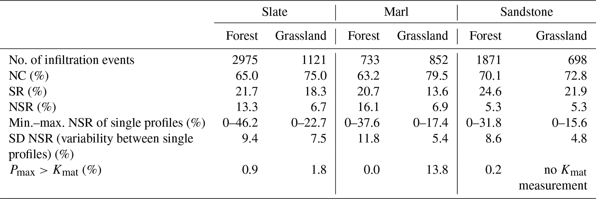
To estimate how often PF should have to be observed based on the classical assumption that rainfall intensity exceeded matrix infiltration capacity in the different landscape units, we calculated the portion of rainfall events with a Pmax exceeding Kmat. With the exception of marl grassland (13.8 % ), all other landscape units only showed an exceedance rate lower than 2 % (Table 3).
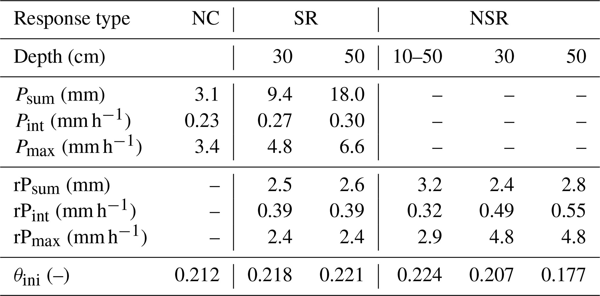
To test how much P characteristics and θini influence the different response behaviors, we calculated the median of each parameter for all infiltration events of a certain response type and their corresponding depth (Table 4). We included pre-response P characteristics (rP) to show their differences between NSR and SR events. High Psum mainly affect the depth of the soil moisture front during SR. In addition, Pmax also increases with depth of response, which could partly be due to a correlation of Pmax and Psum (Spearman R=0.54). SR events show similar median θini values for both infiltration depths, which suggests no effect of θini on the flow depth. The rPsum is similar for SR and NSR 30 and 50 cm events, while rPmax is higher for NSR events. NSR10–50, with a response in 10 cm first followed by a 50 cm reaction, shows a different pattern than the other NSR reactions with the lowest rP intensities, but the highest θini and rPsum. In contrast to SR the median θini of the NSR events is lower and also decreases with increasing depth of the first response (30, 50 cm), which indicates that this infiltration response type is sensitive to dry soil moisture conditions.
Table 4Rainfall characteristics of the different infiltration types and their corresponding depths (median values of all profiles and events). Sequential response (SR) with maximum response depth (cm) and non-sequential response (NSR) with depth of first out-of-sequence response (cm). Rainfall variables were calculated for the entire event (P) and also for the time prior the first (out-of-sequence) sensor response (rP).
Water content change
To estimate the relevance of the different response types in terms of the transported water quantity through the soil, the maximum change in water content for every event (Δθmax) has been taken as a proxy which can further indicate differences in response properties. The patterns of Δθmax in each geology were compared among response type and depth. Figure 4 shows violin plots with Δθmax at the two individual depths during SR. For SR the plots include all events that show a response at the respective depth, independent of the maximum response depth. For NSR 30 and 50 cm events only Δθmax of the first response depth was considered at the respective depth. For NSR10–50 only the water content change in 50 cm (first out-of-sequence reaction) was taken into account. Observed median Δθmax values range between 1.8 vol % and 4.3 vol %. For the SR events, a significant decrease in Δθmax with depth was observed for slate and sandstone sites. Marl sites did not show this damping of the water content signal with depth and exhibited a significant increase in Δθmax at 50 cm depth (SR). For the NSR events no damping of Δθmax with depth was observed. In contrast, NSR in sandstone and marls both had higher Δθmax at 50 cm depth compared to 30 cm. Furthermore, for all geologies Δθmax at NSR 50 cm was similar or even stronger than for NC∕SR 10 cm or SR 30 cm responses.
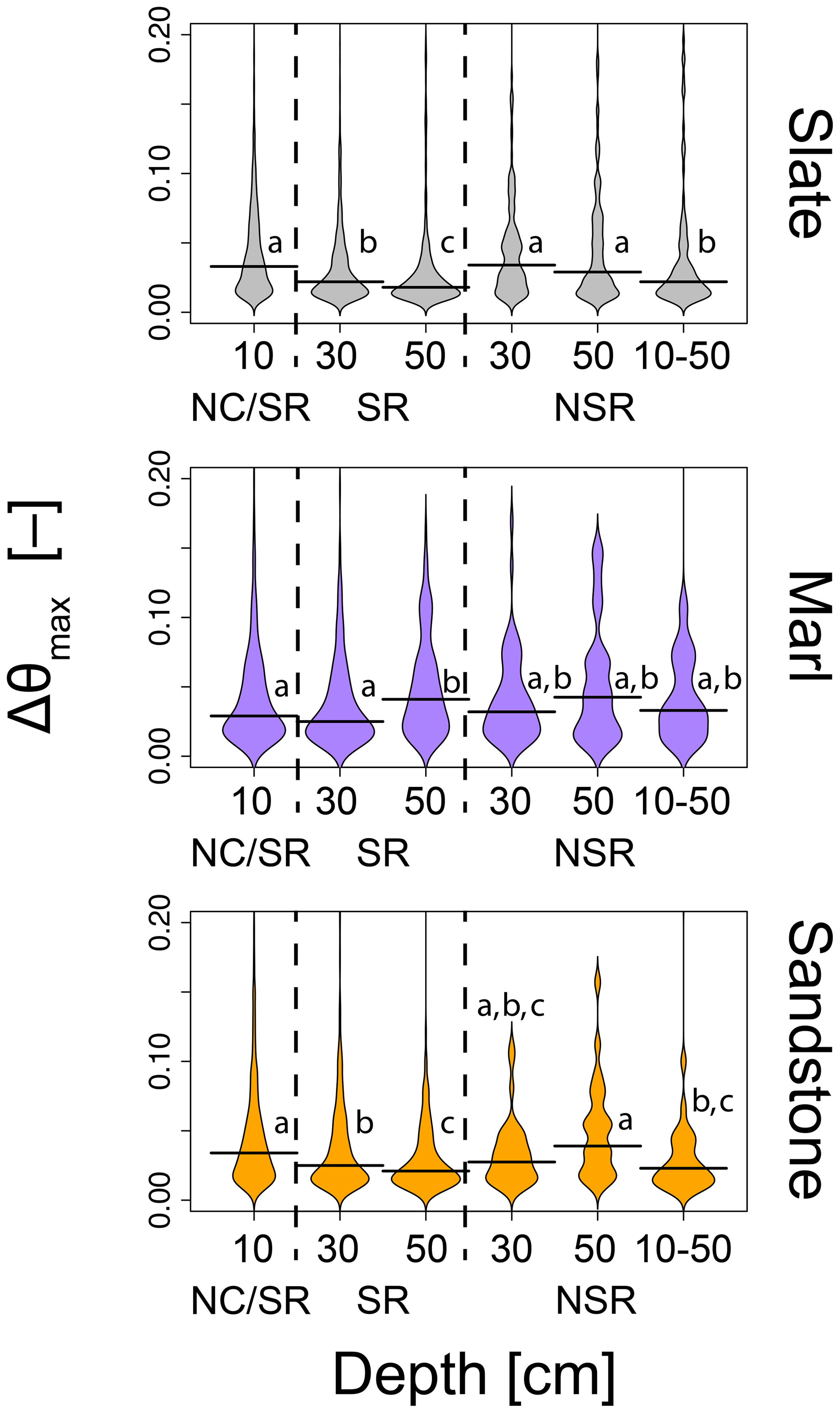
Figure 4Violin plots of maximum volumetric soil moisture change (Δθmax) per depth for the three geologies and differentiated by infiltration response. Δθmax at 10 cm could result from a NC response (10 cm only) or a SR that ends at a deeper sensor (30 or 50 cm). Horizontal lines in the plot indicate the median Δθmax. Same letters symbolize no significant difference between the response classes of the same geology (Dunn test, two-sided, Benjamini–Hochberg correction, p>0.025).
3.2 Non-sequential response (NSR)
The fraction of NSR events in dependence of θini and P characteristics was analyzed to reveal the spatial and temporal patterns and possible controls of PF. Pmax and θini of each profile are only weakly correlated (median profile Spearman R: −0.19). An increase in NSR with increasing rPmax was observed (Fig. 5). Especially forested sites in the slate and marl region showed a strong increase in NSR above a threshold of rP mm h−1. This pattern was only weakly pronounced for the grassland sites. More NSR with higher rPmax in the forests was also found when using maximum rainfall intensity for the whole event (P) instead of the pre-response characteristics (rP).
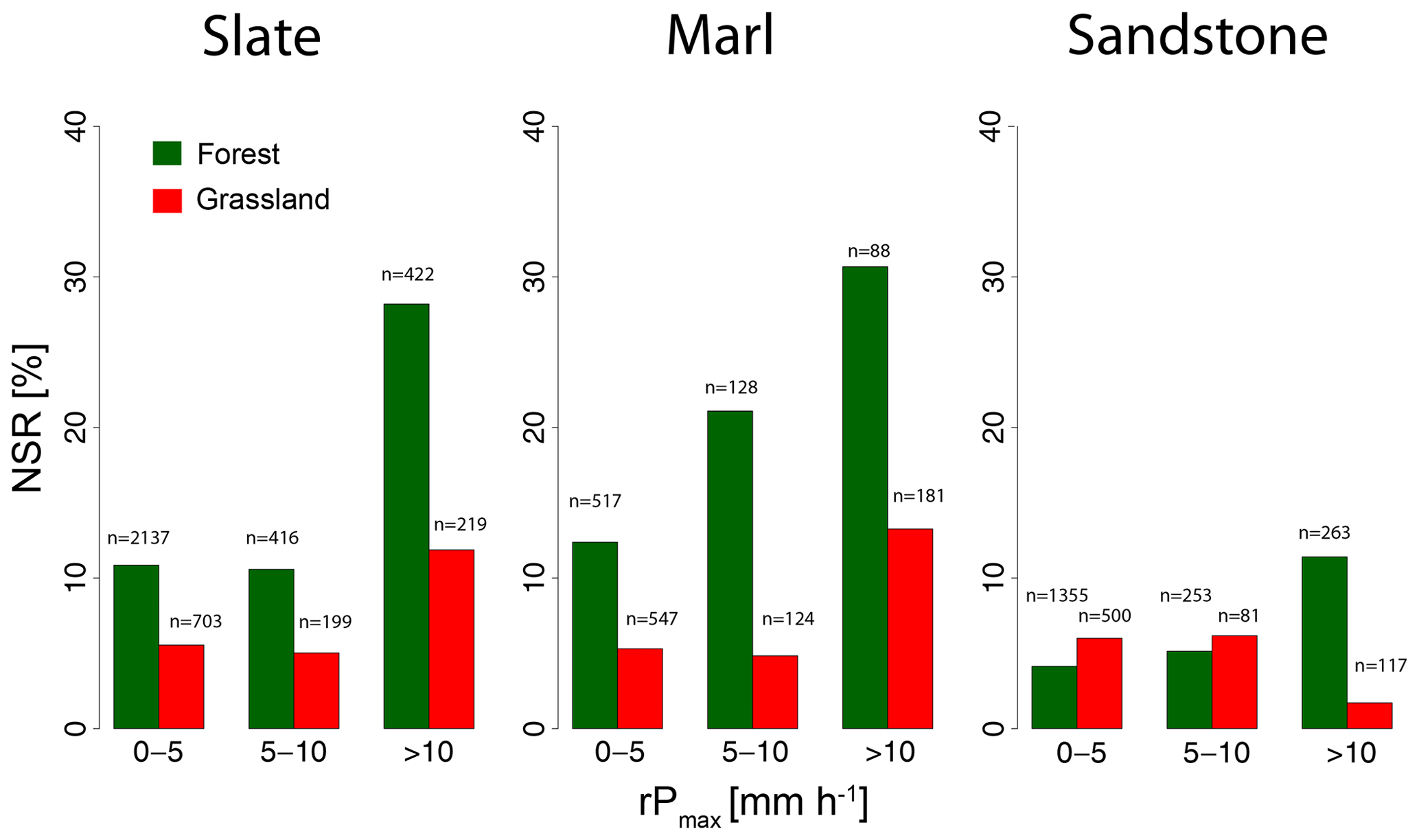
Figure 5NSR vs. rPmax. The numbers above the bars (n) indicate the number of events per class.
Figure 6 shows the portion of NSR response for the six different landscape depending on individual θini quartiles for every profile to account for the differences in absolute θini values among landscape units. We observed that the drier the forested sites were, the higher the measured NSR occurrence was. Especially slate and marl sites showed a strong increase in NSR occurrence (up to ∼25 % of events) for the driest θini quartile. At slate grassland sites observed NSR occurrence was not responding to drier conditions in the same way as for the forested sites. The fraction of NSR events at the marl grassland sites did not change with initial conditions and at sandstone grassland sites NSR occurrence increased only under wetter conditions.

Figure 6Relationship of NSR with θini for each landscape unit. Every point represents % NSR for all events which fall in the four different quartiles of initial soil moisture (the plotting position of θini value represents a quartile median). Number of events observed in the different classes can be found in the Supplement (Table S4).
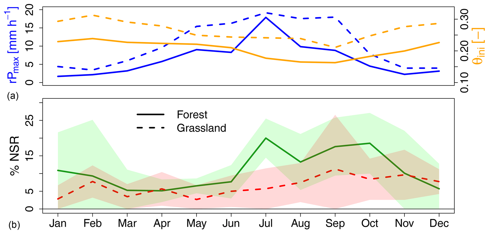
Figure 7Monthly mean rPmax and θini (a) and fraction of NSR events for the two land covers (b). The solid lines represent the forest and the dotted lines the grassland response. The shaded areas in the lower diagram show the standard deviation between the single years for each month. For the number of events observed in the individual month over the total time period and for individual years, see the Supplement (Table S5).
To test for a seasonal effect on the NSR occurrence we also analyzed the frequency of NSR on a monthly basis. Since land cover seems to play an important role for NSR occurrence (Figs. 5 and 6) the NSR portion for all infiltration events of the two land covers was calculated separately. Forests show a distinct seasonal dynamics (Fig. 7): from March to June NSR showed a constant value slightly higher than 5 % which increases to 13 %–20 % from July until October and decreases again towards winter. In the same time period θini dropped to its lowest annual values and rPmax also had its maximum in the summer months. For grasslands this dynamic was less pronounced, with the highest value in September.
3.3 Sequential responses (SR) and flow velocities
3.3.1 Estimating PF by comparison with modeled and measured matrix flow
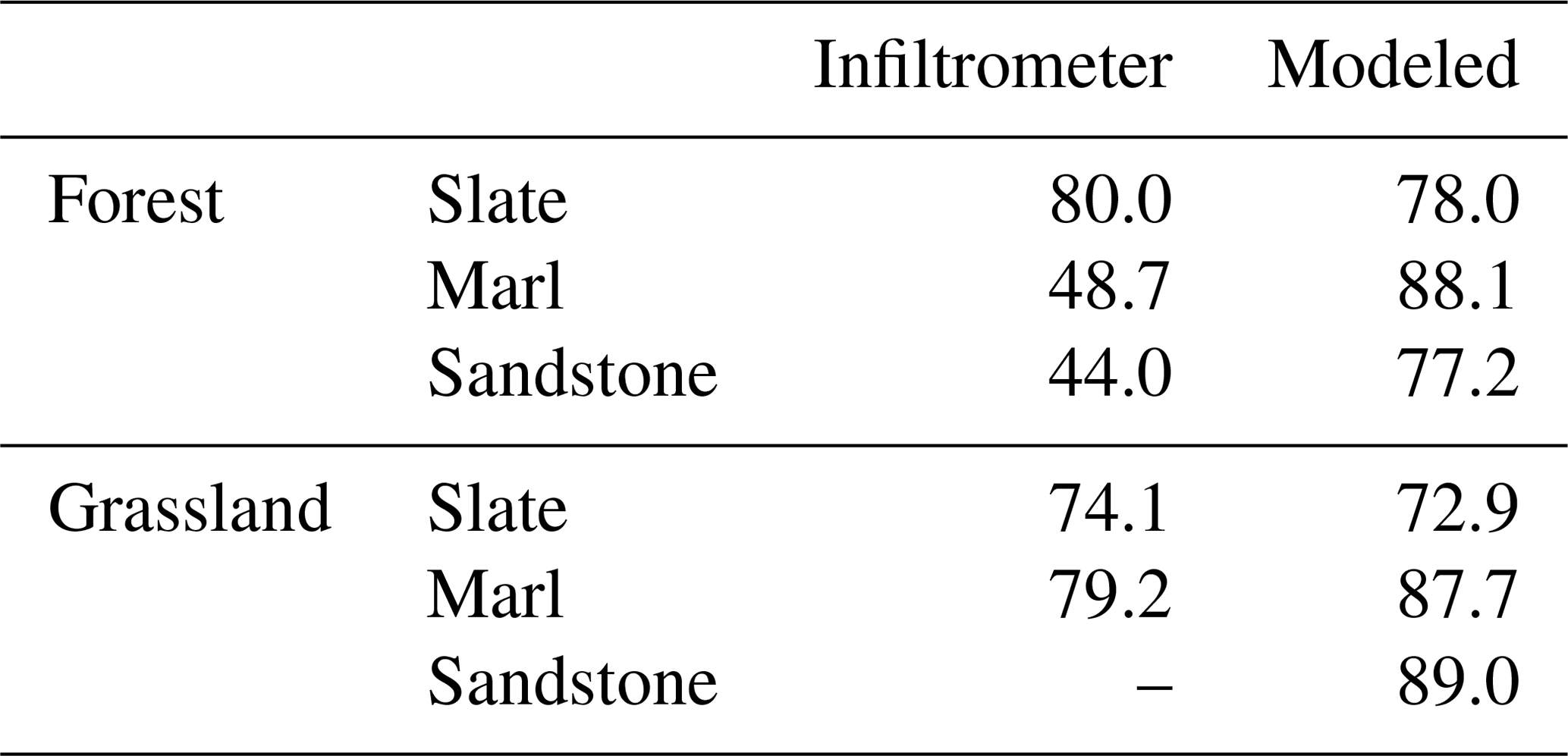
To identify PF from SR, we further compared measured maximum porewater velocities (vmax) against measured (hood infiltrometer, Kmat) and modeled matrix flow velocities (vmat). Table 5 indicates the percentage of observed vmax that exceeds either the measured infiltrometer or modeled values. Both comparisons indicate that observed water flow is in most of the cases faster than water that is flowing in the soil matrix only. Between 72.9 % and 89.0 % of the observed SR responses are faster than the modeled matrix flow velocities. The median difference in flow velocity for the events with is 114 cm d−1. The model matches the exceedance obtained by the hood infiltrometer, except for marl and sandstone forest sites, with an exceedance rate of the infiltrometer being only 48.7 % and 44.0 %, respectively. This is due to the high surface Kmat values that were measured with the hood infiltrometer for these two landscape units. The high conductive parameters of these two landscape units were not distinct higher in the set of hydraulic parameters used for modeling.
Table 5Percentage of event with measured vmax exceeding the infiltrometer (Kmat) or modeled matrix flow velocities (vmat).
3.3.2 Observed maximum porewater velocities
Since the vmax observed from soil moisture responses (SR) exceeded the modeled or measured matrix values most of the time we examined vmax in more detail. The measured vmax ranged from 6 to 80 640 cm d−1 with a median of 120 cm d−1. Only a weak correlation was found between vmax of the shallow versus the deeper depths (10–30 to 30–50 cm; Spearman-R: 0.36). Median observed vmax values per group ranged between 72 cm d−1 for forested sandstone sites (for the shallow depth 10–30 cm) and 274 cm d−1 for forested marl sites (for the depth 30–50 cm) (Fig. 8). Comparing vmax for all landscape units the marl soils showed more variable flow velocities and higher median values, especially between 30 and 50 cm soil depth. Slate soils do not show a significant difference between the two depths or the land covers. Sandstone exhibited highest flow velocities under grassland sites. Forested sandstone soils had a significant lower SR flow velocity than all other soils.
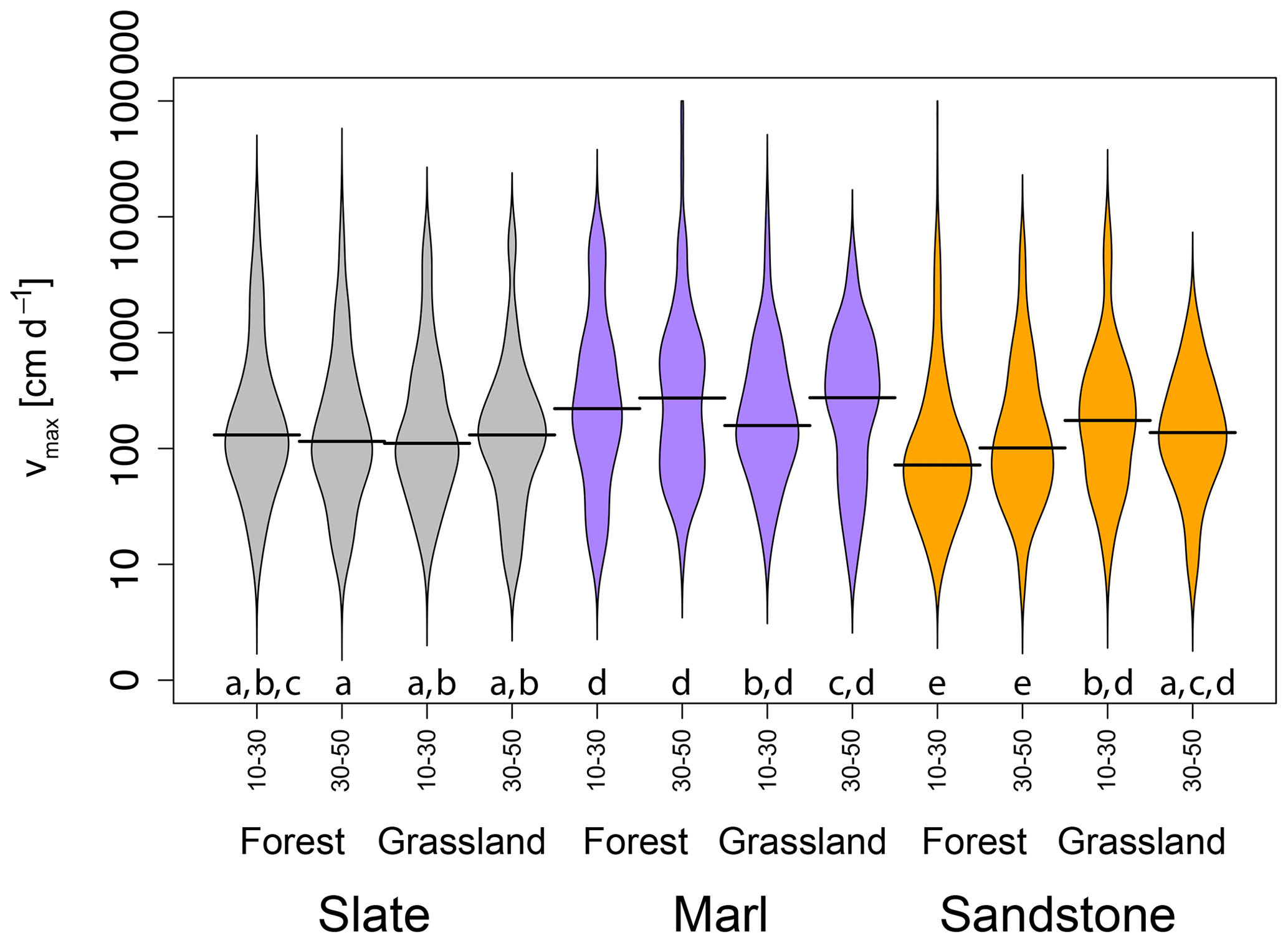
Figure 8Violin plot of observed vmax for the six landscape units (colors) and two depths (10–30, 30–50 cm). Same letters below the plots symbolize no significant difference (p<0.025, Dunn test, two-sided, Benjamini–Hochberg correction).
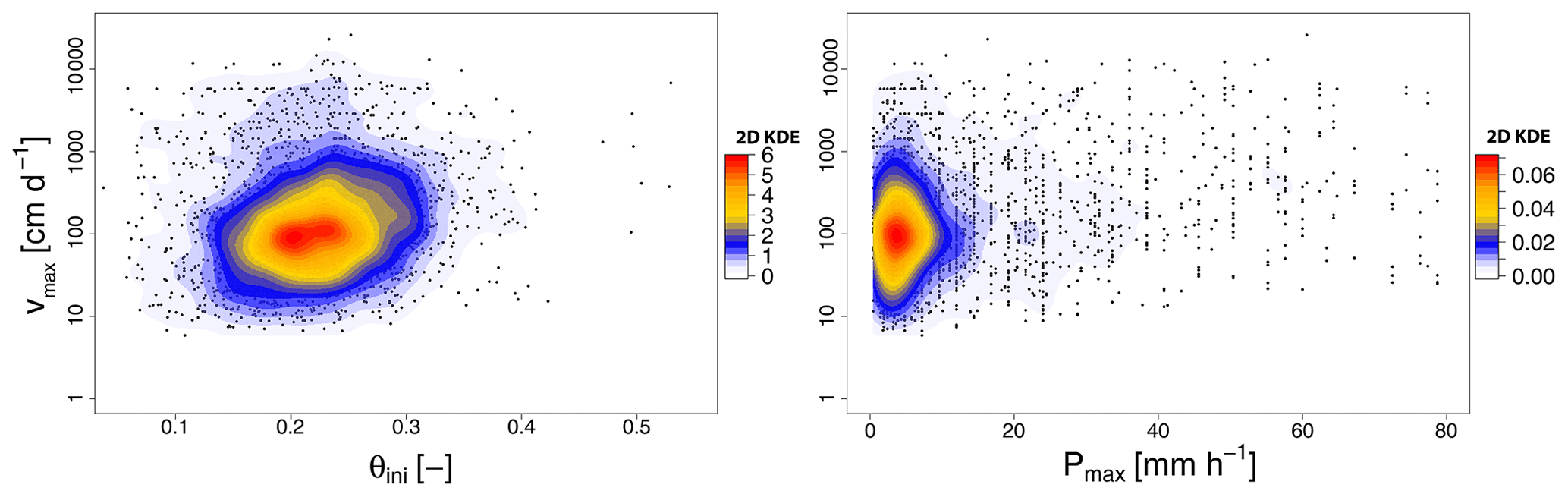
Figure 9Measured SR maximum porewater velocities (vmax) in relation to θini and Pmax. Color contours indicate 2-D kernel density estimation (2-D KDE). The points show single event values.
To further evaluate the variability of vmax with respect to θini and Pmax for all observed events, 2-D kernel density estimations (KDEs) (Venables and Ripley, 2002) are shown in Fig. 9, with higher KDE values indicating more events. There is no clear relationship of vmax with θini or Pmax, and high maximum porewater velocities can be found over the full range of θini and Pmax.
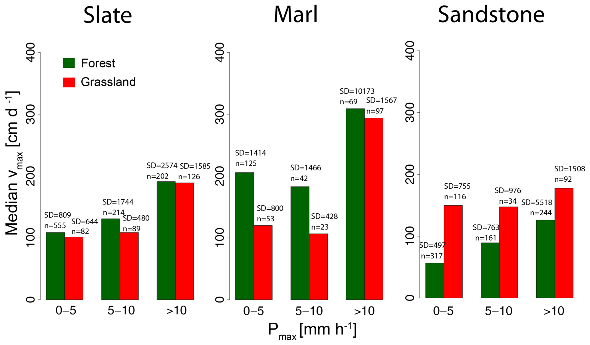
Figure 10Median vmax vs. Pmax. The numbers above the bars indicate the number of events included in the analysis (n) and the standard deviation (SD).
Analyzing the median response of vmax to θini and Pmax for the different landscape units, we can see an increase in median vmax for high Pmax for most landscape units (Fig. 10). Furthermore, the median vmax is increasing under dry conditions for marl independent of land cover and for slate grassland (Fig. 11). The other landscape units do not show a clear pattern between vmax and θini.
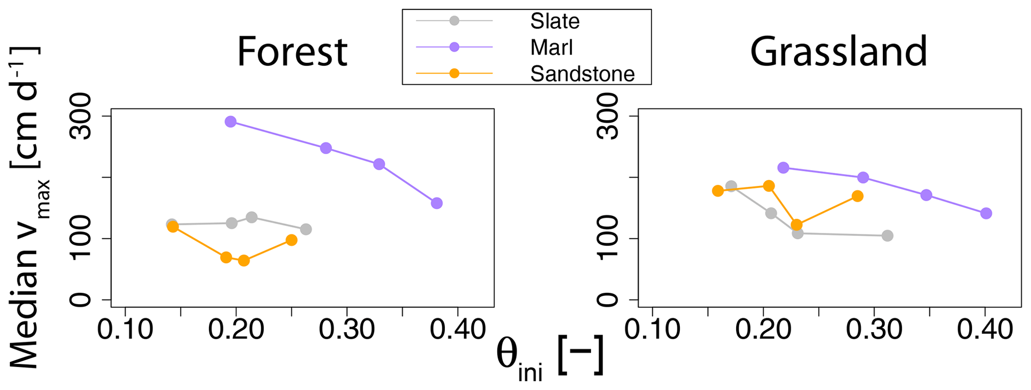
Figure 11Relationship of median vmax with θini for each landscape unit. Each point represents median vmax for all events which fall in the four different quartiles of initial soil moisture (the plotting position of θini value represents a quartile median). Number of events observed in the different classes can be found in the Supplement (Table S6).
Although the relationship of vmax with Pmax and θini is not as clear as with NSR, the seasonal dynamics of median vmax shows an increase during the summer months, with the highest flow velocities during times with low θini and high Pmax. In contrast to NSR, grasslands showed a stronger increase than forests with a maximum between June and August and a median vmax between 225 and 325 cm d−1. For forests a weaker increase in the time between July and August and a stable median vmax of around 200 cm d−1 were seen. The number of observed events furthermore indicates that most SR events are not observed during the times of high vmax, but rather during the wet winter month.
4.1 General relevance of PF
PF as either non-uniform flow (NSR) or as fast sequential flow was observed in all landscape units and under all event conditions (Pmax, θini). The importance of PF during infiltration was highlighted by the fact that observed SR flow velocity (vmax) was most of the time faster than pure soil matrix flow and depended on the landscape unit NSR accounted for 18 %–44 % of the responses deeper than 10 cm. The variability of response types within the landscape units and even within some sites was high, which highlights soil heterogeneity on such larger scales and shows the influence of small-scale soil properties on soil water flow. However, despite the strong variability we found that PF occurrence was dependent on some spatial and temporal factors which are discussed in Sects. 4.4 and 4.5.
PF is important not only in terms of its occurrence frequency, but is also relevant for the quantity of transported water as indicated by the observed water content changes (Δθmax). Especially during NSR the Δθmax is higher than Δθmax for SR at the same depth, which implies fast flow of large amounts of water into deeper zones. Furthermore, the marl sites with their high velocities at 50 cm depth also showed the strongest Δθmax increase at this depth, unlike the other geologies. Similar observations were made by Hardie et al. (2013), who found higher Δθmax at greater depth during NSR or events with high and Eguchi and Hasegawa (2008) calculated that high amounts (16 % to 27 %) of the total annual drainage were produced by PF.
4.2 Observed non-uniform flow (NSR)
In our study, occurrence of NSR for single soil moisture profiles (0 %–46.2 %) was similar to other studies. Liu and Lin (2015) found profile NSR occurrence varying between <1 % and 72.4 % for single years, Graham and Lin (2011) found 18 % to 54 % for a 3-year period and Wiekenkamp et al. (2016) found 7 %–51 % also using a 3-year time series. However, we found a lower average NSR occurrence (mean of the profiles within one landscape unit) of 5.9 %–14.6 % for the landscape units in our study (data not shown) compared to 26 % in the Shale Hills catchment of Graham and Lin (2011). Until now, most studies on NSR events from soil moisture time series focused on a relatively similar substrate (shale), land cover (forest) and a temperate climate (Graham and Lin, 2011; Lin and Zhou, 2008; Liu and Lin, 2015; Wiekenkamp et al., 2016). The slate forest of our study is the landscape unit most comparable to the studies cited above. It shows a comparable range of NSR occurrence (0 %–46.2 % for a single profile). As our experimental design targeted not one but six different landscape units, we were able to compare responses observed in the shale forest to other environments. Sandstone grassland showed a maximum NSR at a single profile of only 15.6 % of the events. Soil profiles under forest on clayey soils (slate and marl) had a higher occurrence of NSR (based on the landscape units) and a higher maximum NSR occurrence for single profiles within these landscape units compared to sandstone or grassland sites. Zhao et al. (2012) also found that a difference in land cover (forest vs. cropland) and soil characteristics affects NSR occurrence. They found lower values with 5.8 %–32.4 % NSR in the croplands compared to the nearby Shale Hills forest, but as the geology differs between the sites, the lower NSR cannot be unequivocally attributed to land cover.
4.3 Observed maximum porewater velocities
Maximum porewater velocities (vmax) in this study (6–80 640 cm d−1) are in the same range as observed in other studies; however, we measured slightly lower median vmax (120 cm d−1) than other studies (e.g., Germann and Hensel, 2006; Hardie et al., 2013; Nimmo, 2007). In addition, studies that measured vmax in single sprinkling experiments in the slate forest region of the Attert catchment observed a vmax of 864–19 000 cm d−1 using GPR and TDR during a hillslope irrigation experiment with an intensity of 30.8 mm h−1 (Angermann et al., 2017). Jackisch et al. (2017) observed vertical transport velocities of bromide in the range of 2732 cm d−1 with sprinkling intensities of 30 and 50 mm h−1. The highest vmax of the slate forest landscape unit measured in our study was with 14662 cm d−1 in a similar range.
Most of the studies mentioned above are sprinkling experiments which apply high P intensities (>10 mm h−1) and high Psum and thus do not provide information on the response to low-intensity events that make up a large portion of the annual rainfall events (see Fig. 3). In his review, Jarvis (2007) found that solute transport studies were either carried out at (near-)saturated conditions or with high irrigation rates (>10 mm h−1). Langhans et al. (2011) found an increase in infiltration capacity with higher rainfall intensity, probably due to the initiation of more macropore flow. This could be an explanation for the higher velocities found by high-intensity sprinkling experiments. Therefore, a reason for the partly lower vmax observed in this study might be that we are also accounting for low P intensity events due to our focus on natural rainfall events. This assumption is supported by the fact that Hardie et al. (2013) measured a vmax of 24–960 cm d−1 under natural rainfall conditions, which is more in the range of most velocities observed in our study. In summary, it is remarkable that no clear differences in flow velocities between different soil types could be identified (neither in our study nor across all previous studies). Instead, all soil types showed a similarly large range of velocities (100–105 cm d−1). Furthermore, one can see orders of magnitude difference in vmax between different events, but not among the landscape units. A clear reduction of maximum porewater velocity with decreasing θ (dry soils) as predicted by conventional unsaturated hydraulic conductivity relationships (e.g., van Genuchten, 1980) was not observed under field conditions. In contrast, higher flow velocities during the driest conditions were observed for most profiles in our study.
4.4 Temporal controls of PF
We found that both, a low initial soil moisture (θini) and a high maximum rainfall intensity (Pmax) affect the occurrence of PF. This results in a higher occurrence of PF during summer time. Increased PF (NSR, vmax) during low θini is in contrast to the classical assumption of PF, which should be initiated more often under wet initial conditions with a lower infiltrability. Furthermore, the mismatch of measured PF occurrence (NSR, fast vmax) compared to the prediction based on Pmax exceeding Kmat indicates that initiation processes such as hydrophobicity/water repellency, local microtopographic depressions or channeling of water by vegetation could be the reason of the frequent occurrence of PF (Blume et al., 2008; Doerr et al., 2000; Schwärzel et al., 2012; Weiler and Naef, 2003). Locally, these processes can lead to higher water contents and thereby pressures at the soil surface close to atmospheric pressure which in turn trigger PF. The higher probability of NSR under dryer conditions and with higher P intensities was also found by Wiekenkamp et al. (2016), Hardie et al. (2013) and Liu and Lin (2015). Also, Hardie et al. (2011) found faster flow velocities under dry conditions, which they concluded was due to hydrophobicity and resulting finger flow, and Blume et al. (2009) found the response time of soil moisture and thereby flow velocity to be much faster during summer time. However, Buttle and Turcotte (1999) did not find a relationship of PF with initial soil water content, but with throughfall intensity.
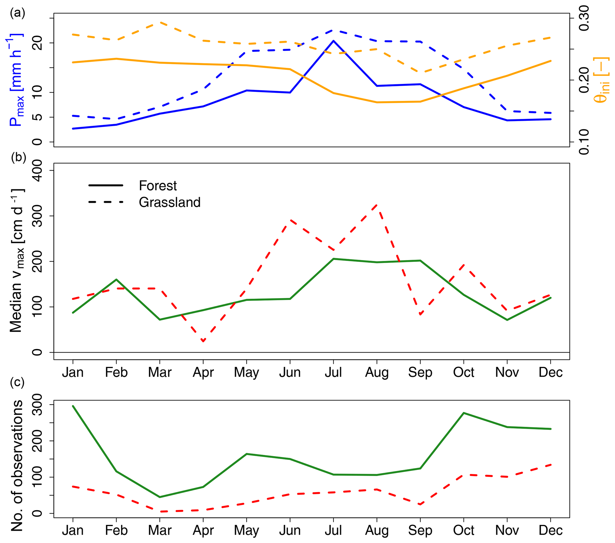
Figure 12Monthly meanPmax and θini (a), monthly median vmax for the two land covers (b) and number of observed vmax values (SR that reached either 30 or 50 cm) for each land cover and month (c). The solid lines represent the forest and the dotted lines the grassland response.
Due to the strong seasonal variation with a PF maximum in summer and early autumn (Figs. 7 and 12), the most probable explanation is the influence of water repellency that has frequently been observed on natural surfaces in summer (Doerr et al., 2006; Täumer et al., 2006). Water repellency hinders infiltration and ensures a pressure buildup at the soil surface until pressure reaches a positive water entry potential (Bauters et al., 2000). Gimbel et al. (2016) observed that their clayey and loamy plots developed strong water repellency during a simulated drought field experiment with a 40-year return period and that infiltration patterns changed from homogeneous to preferential flow. Also, sandy soils were found to be strongly affected by water repellency (e.g., Ritsema et al., 1997). Wessolek et al. (2008) found from 1-year TDR measurements on a pine stand that PF is minor from February to April since the soil was not water repellent. They found a maximum of PF from May to September which matches in general with our observations, just that our observed maximum starts and ends approximately 1 month later. Furthermore, Täumer et al. (2006) observed a similar seasonal pattern over a 3-year period with a maximum of PF in summer and early autumn, and Rye and Smettem (2015) also observed a similar seasonality in Australia. That during these dry and water-repellent conditions the P intensity is highest further supports the initialization of PF. In general higher P intensities can lead to water pressures at the soil surface close to the water entry potential (Gjettermann et al., 1997; Jarvis, 2007; Weiler and Naef, 2003).
4.5 Spatial controls of PF
4.5.1 Clay content
Examining the temporal effects of θini and Pmax between the landscape units in detail, PF dynamics were not the same throughout all landscape units in our study. Especially PF occurrence on clayey soils seems to be strongly influenced by low θini, and a higher clay content enhances NSR occurrence and vmax. Many studies showed that the clay content increases macroporosity under dry conditions through shrinkage and the subsequent cracking of the soil (e.g., Li and Zhang, 2011; Novák, 1999; Stewart et al., 2016a). Das Gupta et al. (2006) measured high infiltration capacity for the macropore domain of clay soils using a tension infiltrometer. The higher macroporosity of the clay soil can then further enhance the occurrence of PF, initialized by higher Pmax and hydrophobic condition in summer as observed by (dye) tracers, infiltration and soil moisture measurements (Dekker and Ritsema, 1996; Hardie et al., 2011; Jarvis et al., 2008). Liu and Lin (2015) found clay content to be an important predictor of NSR in the Shale Hills catchment and we also measured higher NSR in clayey landscape units (slate, marl). Furthermore, we found high maximum pore water velocities in the clay rich subsoil of the marl sites. High vmax in the marl topsoil (lower clay content) is probably more attributed to the high abundance of biopores observed in the topsoil of this region. The high flow velocities in the subsoil are in accordance to other studies that showed fastest velocities due to structure development in unsaturated clay soils (Baram et al., 2012; Hardie et al., 2011; Tiktak et al., 2012). Probably ponding of water on top of the clay layer and subsurface initiation of macropore flow could be a reason of higher flow velocities in the subsoil (Weiler and Naef, 2003). Such a process was observed in the field by Hardie et al. (2011). This demonstrates that in the unsaturated zone close to the surface, clay should not be treated as a low conductivity but rather as a high conductivity material.
4.5.2 Land cover
The question arises why NSR is much more often observed in forests during summer compared to grassland and why vmax is higher in grassland. In general, forests tend to have highly connected macroporosity caused by roots (Alaoui et al., 2011; Gonzalez-Sosa et al., 2010; Lange et al., 2009). Furthermore, higher soil organic carbon content in forest can enhance aggregate stability and hence interaggregate porosity in clayey soil (Lado et al., 2004; Six et al., 2002). However, the sole presence of a higher macroporosity in forests does not explain the higher NSR occurrence. That higher macroporosity results in more NSR could also be caused by more laterally directed pathways in forests created by roots as observed by Bachmair et al. (2009). Funneling of rainfall by stemflow (not measured in this study) may support this mechanism (Schwärzel et al., 2012). In contrast, the stronger increase in vmax in grasslands during summer could be an indication of a seasonally changing macroporosity due to high temporal variation of biopores created by the soil fauna (e.g., earthworms), as observed in our study region (Schneider et al., 2016). Biopores such as earthworm burrows were frequently found to enhance vertical PF (Reck et al., 2018; Weiler and Flühler, 2004; Zehe and Flühler, 2001).
Our results demonstrate that infiltration is strongly controlled by PF phenomena. As expected a higher maximum rainfall intensity increases the occurrence of PF, but different from common theory a higher soil moisture decreases the PF occurrence. However, the here studied landscape units show a high spatial heterogeneity and high temporal variation with different PF processes involved, such as more fast PF in grasslands and more non-uniform flow (NSR) in forest. Clay-rich soils showed to increase both, non-uniform PF (NSR) and fast PF (high vmax). By systematically comparing the dynamics of different landscape units we were able to identify that beside the amount of connected macropores such as cracks (influenced by a high clay content and low soil moisture) or biotic macropores (roots channels, earthworm borrows), PF strongly depends on initiation processes (water repellency, rain intensity). This leads to a strong seasonal dynamics with more non-uniform flow and highest flow velocities in summer and early autumn due to dry soils, high rainfall intensities and hydrophobic soil surfaces. Furthermore, the amounts of transported water are higher during non-uniform flow. This can have a potential impact on solute transport during summer months and should be considered in water management.
We were able to show that soil texture is not the main driver of water flow velocity during infiltration in the vadose zone as we typically assume. We suggest including dynamic flow processes, dynamic initialization processes and varying macroporosity in physically based hydrological models rather than static hydraulic conductivities derived from soil cores or soil maps. Therefore it needs easily transferable relationships or pedotransfer functions, which can help to find structure-related PF parameters similar to retention parameters. More effort is necessary to find or adapt already existing approaches to measuring and monitoring PF in diverse landscapes. We further suggest implementing large-scale sensor networks under different climatic settings, substrates, topographies, and land covers worldwide and creating standardized approaches for analyzing soil moisture datasets. Our approach can be expanded by combining it with groundwater response time series and stable isotope methods to identify and understand flow patterns in the vadose zone at the landscape scale.
Data and the analysis code are available from the authors upon request.
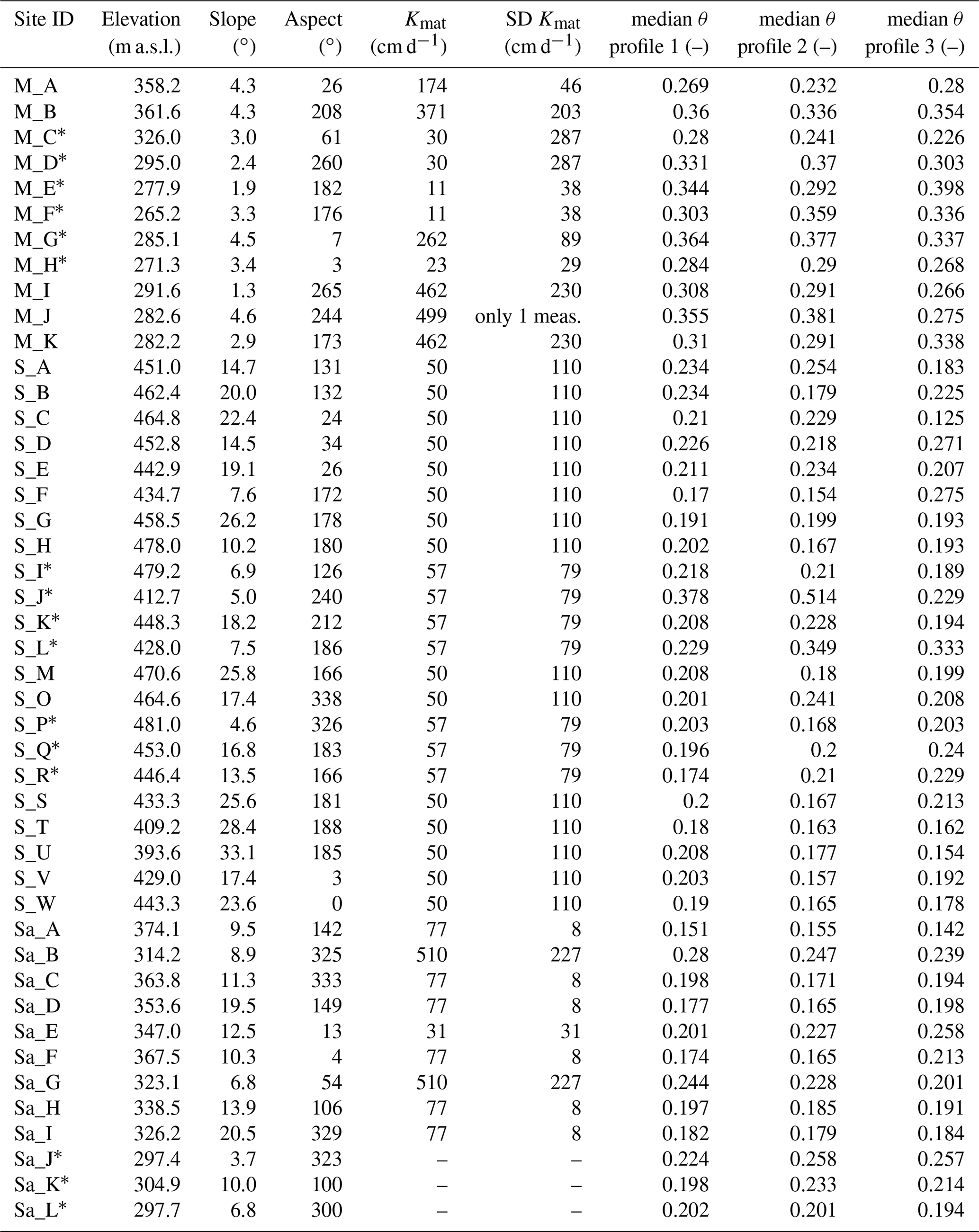
Table A1S: slate; M: marl; Sa: sandstone. ∗ indicates grassland sites. SD: standard deviation.
The supplement related to this article is available online at: https://doi.org/10.5194/hess-23-4869-2019-supplement.
DD prepared the data, developed and performed the analysis strategy and planned and conducted the fieldwork. MW and TB designed the sensor cluster setup, were involved in their installation and contributed to the data analysis strategy. DD prepared the manuscript with contributions from all the co-authors.
The authors declare that they have no conflict of interest.
This article is part of the special issue “Linking landscape organisation and hydrological functioning: from hypotheses and observations to concepts, models and understanding (HESS/ESSD inter-journal SI)”. It is not associated with a conference.
Special thanks to Britta Kattenstroth, Tobias Vetter, Sibylle Hassler and many other helpers for the installation and maintenance of the field sites. We thank Conrad Jackisch for partly providing the soil and infiltration data and Natalie Orlowski for the helpful comments on the manuscript. We acknowledge the comments of Heye Bogena, Nicholas Jarvis and two anonymous reviewers which greatly improved this paper.
This research has been supported by the German Research Association (DFG; grant no. FOR 1598 – From Catchments as Organized Systems to Models based on Dynamic Functional Units – CAOS). The article processing charge was funded by the German Research Foundation (DFG) and the University of Freiburg in the Open Access Publishing funding program.
This paper was edited by Hjalmar Laudon and reviewed by Heye Bogena, Nicholas Jarvis, and two anonymous referees.
Abbaspour, K. C., Johnson, C. A., and van Genuchten, M. T.: Estimating Uncertain Flow and Transport Parameters Using a Sequential Uncertainty Fitting Procedure, Vadose Zone J., 3, 1340–1352, https://doi.org/10.2136/vzj2004.1340, 2004.
Alaoui, A., Caduff, U., Gerke, H. H., and Weingartner, R.: Preferential Flow Effects on Infiltration and Runoff in Grassland and Forest Soils, Vadose Zone J., 10, 367–377, https://doi.org/10.2136/vzj2010.0076, 2011.
Allaire, S. E., Roulier, S., and Cessna, A. J.: Quantifying preferential flow in soils: A review of different techniques, J. Hydrol., 378, 179–204, https://doi.org/10.1016/j.jhydrol.2009.08.013, 2009.
Anderson, A. E., Weiler, M., Alila, Y., and Hudson, R. O.: Dye staining and excavation of a lateral preferential flow network, Hydrol. Earth Syst. Sci., 13, 935–944, https://doi.org/10.5194/hess-13-935-2009, 2009.
Angermann, L., Jackisch, C., Allroggen, N., Sprenger, M., Zehe, E., Tronicke, J., Weiler, M., and Blume, T.: Form and function in hillslope hydrology: characterization of subsurface flow based on response observations, Hydrol. Earth Syst. Sci., 21, 3727–3748,https://doi.org/10.5194/hess-21-3727-2017, 2017.
Arora, B., Mohanty, B. P., and McGuire, J. T.: Inverse estimation of parameters for multidomain flow models in soil columns with different macropore densities, Water Resour. Res., 47, 1–17, https://doi.org/10.1029/2010WR009451, 2011.
Bachmair, S., Weiler, M., and Nützmann, G.: Controls of land use and soil structure on water movement: Lessons for pollutant transfer through the unsaturated zone, J. Hydrol., 369, 241–252, https://doi.org/10.1016/j.jhydrol.2009.02.031, 2009.
Baram, S., Kurtzman, D., and Dahan, O.: Water percolation through a clayey vadose zone, J. Hydrol., 424–425, 165–171, https://doi.org/10.1016/j.jhydrol.2011.12.040, 2012.
Bauters, T. W. J., Steenhuis, T. S., Dicarlo, D. A., Nieber, J. L., Dekker, L. W., Ritsema, C. J., Parlange, J. Y., and Haverkamp, R.: Physics of water repellent soils, J. Hydrol., 231–232, 233–243, https://doi.org/10.1016/S0022-1694(00)00197-9, 2000.
Beven, K. and Germann, P.: Macropores and Water Flow in Soils, Water Resour. Res., 18, 1311–1325, 1982.
Beven, K. and Germann, P.: Macropores and water flow in soils revisited, Water Resour. Res., 49, 3071–3092, https://doi.org/10.1002/wrcr.20156, 2013.
Blonquist, J. M., Jones, S. B., and Robinson, D. A.: Standardizing Characterization of Electromagnetic Water Content Sensors, Vadose Zone J., 4, 1059–1069, https://doi.org/10.2136/vzj2004.0141, 2005.
Blume, T., Zehe, E., and Bronstert, A.: Investigation of runoff generation in a pristine, poorly gauged catchment in the Chilean Andes II: Qualitative and quantitative use of tracers at three spatial scales, Hydrol. Process., 22, 3676–3688, https://doi.org/10.1002/hyp.6970, 2008.
Blume, T., Zehe, E., and Bronstert, A.: Use of soil moisture dynamics and patterns at different spatio-temporal scales for the investigation of subsurface flow processes, Hydrol. Earth Syst. Sci., 13, 1215–1233, https://doi.org/10.5194/hess-13-1215-2009, 2009.
Bormann, H. and Klaassen, K.: Seasonal and land use dependent variability of soil hydraulic and soil hydrological properties of two Northern German soils, Geoderma, 145, 295–302, https://doi.org/10.1016/j.geoderma.2008.03.017, 2008.
Buttle, J. M. and McDonald, D. J.: Soil macroporosity and infiltration characteristics of a forest podzol, Hydrol. Process., 14, 831–848, 2000.
Buttle, J. M. and Turcotte, D. S.: Runoff processes on a forested slope on the Canadian Shield., Nord. Hydrol., 30, 1–20, 1999.
Cheng, Y., Ogden, F. L., and Zhu, J.: Earthworms and tree roots: A model study of the effect of preferential flow paths on runoff generation and groundwater recharge in steep, saprolitic, tropical lowland catchments, Water Resour. Res., 53, 5400–5419, https://doi.org/10.1002/2016WR020258, 2017.
Cobos, D.: Application Note – Measurement Volume of Decagon Volumetric Water Content Sensors, Decagon Devices, Pullman, WA, USA, 2015.
Colbach, R. and Maquil, R.: Carte Géologique du Luxembourg – Feuille No. 7 Redange 1 : 25 000, Service Géologique de Luxembourg, Ministère des Travaux Publics, Luxembourg, 2003.
Das Gupta, S., Mohanty, B. P., and Köhne, J. M.: Soil Hydraulic Conductivities and their Spatial and Temporal Variations in a Vertisol, Soil Sci. Soc. Am. J., 70, 1872–1881, https://doi.org/10.2136/sssaj2006.0201, 2006.
DecagonDevices: 5TE Water contant, EC and temperature sensor, Decagon Devices, Inc., Version: March 11, 2016 — 11:55:57, available at: http://manuals.decagon.com/Retired and Discontinued/Manuals/13509_5TE_Web.pdf (last access: 22 November 2019), 2016.
Dekker, L. W. and Ritsema, C. J.: Preferential flow path in a water repellent clay soil with grass cover, Water Resour. Res., 32, 1239–1249, 1996.
DIN ISO 11277: Soil quality – Determination of particle size distribution in mineral soil material – Method by sieving and sedimentation (ISO 11277:1998 + ISO 11277:1998 Corrigendum 1:2002), Beuth Verlag, Berlin, Germany, 2002.
Dinno, A.: dunn.test: Dunn's Test of Multiple Comparisons Using Rank Sums. R package version 1.3.5, available at: https://cran.r-project.org/package=dunn.test (last access: 22 November 2019), 2017.
Doerr, S. H., Shakesby, R. A., and Walsh, R. P. D.: Soil water repellency: Its causes, characteristics and hydro-geomorphological significance, Earth Sci. Rev., 51, 33–65, https://doi.org/10.1016/S0012-8252(00)00011-8, 2000.
Doerr, S. H., Shakesby, R. A., Dekker, L. W., and Ritsema, C. J.: Occurrence, prediction and hydrological effects of water repellency amongst major soil and land-use types in a humid temperate climate, Eur. J. Soil Sci., 57, 741–754, https://doi.org/10.1111/j.1365-2389.2006.00818.x, 2006.
Durner, W.: Hydraulic Conductivity Estimation for Soils with Heterogeneus pore Structure, Water Resour. Res., 30, 211–223, https://doi.org/10.1029/93WR02676, 1994.
Eguchi, S. and Hasegawa, S.: Determination and Characterization of Preferential Water Flow in Unsaturated Subsoil of Andisol, Soil Sci. Soc. Am. J., 72, 320–330, https://doi.org/10.2136/sssaj2007.0042, 2008.
Flury, M., Flühler, H., Jury, W. A., and Leuenberger, J.: Susceptibility of soils to preferential flow of water: A field study, Water Resour. Res., 30, 1945–1954, 1994.
Gardner, W. R.: Some steady-state solutions of the unsaturated moisture flow equation with application to evaporation from a water table, Soil Sci., 85, 228–232, https://doi.org/10.1097/00010694-195804000-00006, 1958.
Gerke, H. H.: Preferential flow descriptions for structured soils, J. Plant Nutr. Soil Sci., 169, 382–400, https://doi.org/10.1002/jpln.200521955, 2006.
Germann, P. F. and Hensel, D.: Poiseuille Flow Geometry Inferred from Velocities of Wetting Fronts in Soils, Vadose Zone J., 5, 867–876, https://doi.org/10.2136/vzj2005.0080, 2006.
Gimbel, K. F., Puhlmann, H., and Weiler, M.: Does drought alter hydrological functions in forest soils?, Hydrol. Earth Syst. Sci., 20, 1301–1317, https://doi.org/10.5194/hess-20-1301-2016, 2016.
Gjettermann, B., Nielsen, K. L., Petersen, C. T., Jensen, H. E., and Hansen, S.: Preferential flow in sandy loam soils as affected by irrigation intensity, Soil Technol., 11, 139–152, https://doi.org/10.1016/S0933-3630(97)00001-9, 1997.
Gonzalez-Sosa, E., Braud, I., Dehotin, J., Lassabatère, L., Angulo-Jaramillo, R., Lagouy, M., Branger, F., Jacqueminet, C., Kermadi, S., and Michel, K.: Impact of land use on the hydraulic properties of the topsoil in a small French catchment, Hydrol. Process., 24, 2382–2399, https://doi.org/10.1002/hyp.7640, 2010.
Graham, C. B. and Lin, H. S.: Controls and Frequency of Preferential Flow Occurrence: A 175-Event Analysis, Vadose Zone J., 10, 816–831, https://doi.org/10.2136/vzj2010.0119, 2011.
Hardie, M., Lisson, S., Doyle, R., and Cotching, W.: Determining the frequency, depth and velocity of preferential flow by high frequency soil moisture monitoring, J. Contam. Hydrol., 144, 66–77, https://doi.org/10.1016/j.jconhyd.2012.10.008, 2013.
Hardie, M. A., Cotching, W. E., Doyle, R. B., Holz, G., Lisson, S., and Mattern, K.: Effect of antecedent soil moisture on preferential flow in a texture-contrast soil, J. Hydrol., 398, 191–201, https://doi.org/10.1016/j.jhydrol.2010.12.008, 2011.
Hendrickx, J. M. H. and Flury, M.: Uniform and preferential flow mechanisms in the vadose zone, in Conceptual models of flow and transport in the fractured vadose zone, Natl. Acad. Press, Washington, D.C., USA, 149–187, 2001.
Hillel, D.: Environmental Soil Physics, Academic Press, London, UK, 1998.
Ireson, A. M. and Butler, A. P.: Controls on preferential recharge to Chalk aquifers, J. Hydrol., 398, 109–123, https://doi.org/10.1016/j.jhydrol.2010.12.015, 2011.
IUSS Working Group WRB: World reference base for soil resources 2006, World Soil Resour. Reports No. 103, FAO, Rome, Italy, 2006.
Jackisch, C., Angermann, L., Allroggen, N., Sprenger, M., Blume, T., Tronicke, J., and Zehe, E.: Form and function in hillslope hydrology: in situ imaging and characterization of flow-relevant structures, Hydrol. Earth Syst. Sci., 21, 3749–3775, https://doi.org/10.5194/hess-21-3749-2017, 2017.
Jarvis, N., Etana, A., and Stagnitti, F.: Water repellency, near-saturated infiltration and preferential solute transport in a macroporous clay soil, Geoderma, 143, 223–230, https://doi.org/10.1016/j.geoderma.2007.11.015, 2008.
Jarvis, N., Koestel, J., Messing, I., Moeys, J., and Lindahl, A.: Influence of soil, land use and climatic factors on the hydraulic conductivity of soil, Hydrol. Earth Syst. Sci., 17, 5185–5195, https://doi.org/10.5194/hess-17-5185-2013, 2013.
Jarvis, N. J.: A review of non-equilibrium water flow and solute transport in soil macropores: Principles, controlling factors and consequences for water quality, Eur. J. Soil Sci., 58, 523–546, https://doi.org/10.1111/j.1365-2389.2007.00915.x, 2007.
Juilleret, J., Iffly, J. F., Pfister, L., and Hissler, C.: Remarkable Pleistocene periglacial slope deposits in Luxembourg (Oesling): pedological implication and geosite potential, Bull. Société des Nat. Luxemb., 112, 125–130, 2011.
Juilleret, J., Iffly, J. F., Hoffmann, L., and Hissler, C.: The potential of soil survey as a tool for surface geological mapping: A case study in a hydrological experimental catchment (Huewelerbach, grand-duchy of Luxembourg), Geol. Belg., 15, 36–41, 2012.
Kim, S., Lee, H., Woo, N. C., and Kim, J.: Soil moisture monitoring on a steep hillside, Hydrol. Process., 21, 2910–2922, https://doi.org/10.1002/hyp.6508, 2007.
Koestel, J. K., Norgaard, T., Luong, N. M., Vendelboe, A. L., Moldrup, P., Jarvis, N. J., Lamandé, M., Iversen, B. V., and Wollesen De Jonge, L.: Links between soil properties and steady-state solute transport through cultivated topsoil at the field scale, Water Resour. Res., 49, 790–807, https://doi.org/10.1002/wrcr.20079, 2013.
Köhne, J. M., Köhne, S., and Šimůnek, J.: A review of model applications for structured soils: (a) Water flow and tracer transport, J. Contam. Hydrol., 104, 4–35, https://doi.org/10.1016/j.jconhyd.2008.10.002, 2009.
Kung, K.-J. S.: Preferential flow in a sandy vadose zone: 1. Field observation, Geoderma, 46, 51–58, https://doi.org/10.1016/0016-7061(90)90006-U, 1990.
Lado, M., Paz, A., and Ben-Hur, M.: Organic Matter and Aggregate-Size Interactions in Saturated Hydraulic Conductivity, Soil Sci. Soc. Am. J., 68, 234–242, https://doi.org/10.2136/sssaj2004.2340, 2004.
Lange, B., Lüescher, P., and Germann, P. F.: Significance of tree roots for preferential infiltration in stagnic soils, Hydrol. Earth Syst. Sci., 13, 1809–1821, https://doi.org/10.5194/hess-13-1809-2009, 2009.
Langhans, C., Govers, G., Diels, J., Leys, A., Clymans, W., Van den Putte, A., and Valckx, J.: Experimental rainfall-runoff data: Reconsidering the concept of infiltration capacity, J. Hydrol., 399, 255–262, https://doi.org/10.1016/j.jhydrol.2011.01.005, 2011.
Larsbo, M., Koestel, J., and Jarvis, N.: Relations between macropore network characteristics and the degree of preferential solute transport, Hydrol. Earth Syst. Sci., 18, 5255–5269, https://doi.org/10.5194/hess-18-5255-2014, 2014.
Li, J. H. and Zhang, L. M.: Study of desiccation crack initiation and development at ground surface, Eng. Geol., 123, 347–358, https://doi.org/10.1016/j.enggeo.2011.09.015, 2011.
Lin, H. and Zhou, X.: Evidence of subsurface preferential flow using soil hydrologic monitoring in the Shale Hills catchment, Eur. J. Soil Sci., 59, 34–49, https://doi.org/10.1111/j.1365-2389.2007.00988.x, 2008.
Lin, H. S., Kogelmann, W., Walker, C., and Bruns, M. A.: Soil moisture patterns in a forested catchment: A hydropedological perspective, Geoderma, 131, 345–368, https://doi.org/10.1016/j.geoderma.2005.03.013, 2006.
Liu, H. and Lin, H.: Frequency and Control of Subsurface Preferential Flow: From Pedon to Catchment Scales, Soil Sci. Soc. Am. J., 79, 362–377, https://doi.org/10.2136/sssaj2014.08.0330, 2015.
Martínez-Carreras, N., Krein, A., Gallart, F., Iffly, J. F., Hissler, C., Pfister, L., Hoffmann, L., and Owens, P. N.: The influence of sediment sources and hydrologic events on the nutrient and metal content of fine-grained sediments (attert river basin, Luxembourg), Water. Air. Soil Pollut., 223, 5685–5705, https://doi.org/10.1007/s11270-012-1307-1, 2012.
Moragues-Quiroga, C., Juilleret, J., Gourdol, L., Pelt, E., Perrone, T., Aubert, A., Morvan, G., Chabaux, F., Legout, A., Stille, P., and Hissler, C.: Genesis and evolution of regoliths: Evidence from trace and major elements and Sr-Nd-Pb-U isotopes, Catena, 149, 185–198, https://doi.org/10.1016/j.catena.2016.09.015, 2017.
Naveed, M., Moldrup, P., Schaap, M. G., Tuller, M., Kulkarni, R., Vogel, H.-J., and Wollesen de Jonge, L.: Prediction of biopore- and matrix-dominated flow from X-ray CT-derived macropore network characteristics, Hydrol. Earth Syst. Sci., 20, 4017–4030, https://doi.org/10.5194/hess-20-4017-2016, 2016.
Nimmo, J. R.: Simple predictions of maximum transport rate in unsaturated soil and rock, Water Resour. Res., 43, 139–141, https://doi.org/10.1029/2006WR005372, 2007.
Novák, V.: Soil-crack characteristics – Estimation methods applied to heavy soils in the NOPEX area, Agr. Forest Meteorol., 98–99, 501–507, https://doi.org/10.1016/S0168-1923(99)00119-7, 1999.
Oberdörster, C., Vanderborght, J., Kemna, A., and Vereecken, H.: Investigating Preferential Flow Processes in a Forest Soil Using Time Domain Reflectometry and Electrical Resistivity Tomography, Vadose Zone J., 9, 350–361, https://doi.org/10.2136/vzj2009.0073, 2010.
Pfister, L., Hoffmann, L., Heitz, S., Iffly, J.-F., Matgen, P., Tailliez, C., Wagner, C., Schoder, R., Buchel, D., Lepesant, P., Wiltgen, C., Frisch, C., Kipgen, R., Ripp, C., and Schleich, G.: Atlas hydro-climatologique du Grand-Duché de Luxembourg 2006, Ministère de l'Agriculture, de la Viticulture et du Développement Rural; Ministère de l'Intérieur et de l'Aménagement du Territoire; Centre de Recherche Public, 2006.
Reck, A., Jackisch, C., Hohenbrink, T. L., Zangerlé, A., and Schaik, L. Van: Impact of Temporal Macropore Dynamics on Infiltration?: Field Experiments and Model Simulations, Vadose Zone J., 17, https://doi.org/10.2136/vzj2017.08.0147, 2018.
Ritsema, C. J., Steenhuis, T. S., Parlange, J. Y., and Dekker, L. W.: Predicted and observed finger diameters in field soils, Geoderma, 70, 185–196, https://doi.org/10.1016/0016-7061(95)00080-1, 1996.
Ritsema, C. J., Dekker, L. W., van den Elsen, E. G. M., Oostindiel, K., Steenhuis, T. S., and Nieber, J. L.: Recurring fingered flow pathways in a water repellent sandy field soil, Hydrol. Earth Syst. Sci., 1, 777–786, https://doi.org/10.5194/hess-1-777-1997, 1997.
Rosenbaum, U., Huisman, J. A., Weuthen, A., Vereecken, H., and Bogena, H. R.: Sensor-to-Sensor Variability of the ECHO EC-5, TE, and 5TE Sensors in Dielectric Liquids, Vadose Zone J., 9, 181–186, https://doi.org/10.2136/vzj2009.0036, 2010.
Rosenbaum, U., Huisman, J. A., Vrba, J., Vereecken, H., and Bogena, H. R.: Correction of Temperature and Electrical Conductivity Effects on Dielectric Permittivity Measurements with ECHO Sensors, Vadose Zone J., 10, 582–593, https://doi.org/10.2136/vzj2010.0083, 2011.
Rosenbaum, U., Bogena, H. R., Herbst, M., Huisman, J. A., Peterson, T. J., Weuthen, A., Western, A. W., and Vereecken, H.: Seasonal and event dynamics of spatial soil moisture patterns at the small catchment scale, Water Resour. Res., 48, 1–22, https://doi.org/10.1029/2011WR011518, 2012.
Rye, C. F. and Smettem, K. R. J.: Seasonal and Interannual Variability of the Effective Flow Cross-Sectional Area in a Water-Repellent Soil, Vadose Zone J., 14, https://doi.org/10.2136/vzj2014.10.0141, 2015.
Schneider, A. K., van Schaik, L., Zangerlé, A., Eccard, J. A., and Schröder, B.: Which abiotic filters shape earthworm distribution patterns at the catchment scale?, Eur. J. Soil Sci., 67, 431–442, https://doi.org/10.1111/ejss.12346, 2016.
Schwärzel, K. and Punzel, J.: Hood Infiltrometer – A New Type of Tension Infiltrometer, Soil Sci. Soc. Am. J., 71, 1438–1447, https://doi.org/10.2136/sssaj2006.0104, 2007.
Schwärzel, K., Menzer, A., Clausnitzer, F., Spank, U., Häntzschel, J., Grünwald, T., Köstner, B., Bernhofer, C., and Feger, K. H.: Soil water content measurements deliver reliable estimates of water fluxes: A comparative study in a beech and a spruce stand in the Tharandt forest (Saxony, Germany), Agr. Forest Meteorol., 149, 1994–2006, https://doi.org/10.1016/j.agrformet.2009.07.006, 2009.
Schwärzel, K., Ebermann, S., and Schalling, N.: Evidence of double-funneling effect of beech trees by visualization of flow pathways using dye tracer, J. Hydrol., 470–471, 184–192, https://doi.org/10.1016/j.jhydrol.2012.08.048, 2012.
Selker, J. S., Leclerq, P., Parlange, J.-Y., and Steenhuis, T. S.: Fingered Flow in Two Dimensions. 1. Measurement of matric potential, Water Resour. Res., 28, 2513–2521, https://doi.org/10.1029/92WR00963, 1992.
Six, J., Conant, R. T., Paul, E. A., and Paustian, K.: Stabilization mechanisms of soil organic matter: Implications for C-saturation of soils, Plant Soil, 241, 155–176, https://doi.org/10.1023/A:1016125726789, 2002.
Sprenger, M., Volkmann, T. H. M., Blume, T., and Weiler, M.: Estimating flow and transport parameters in the unsaturated zone with pore water stable isotopes, Hydrol. Earth Syst. Sci., 19, 2617–2635, https://doi.org/10.5194/hess-19-2617-2015, 2015.
Sprenger, M., Seeger, S., Blume, T., and Weiler, M.: Travel times in the vadose zone: Variability in space and time, Water Resour. Res., 52, 5727–5754, https://doi.org/10.1002/2015WR018077, 2016.
Steinbrich, A., Leistert, H., and Weiler, M.: Model-based quantification of runoff generation processes at high spatial and temporal resolution, Environ. Earth Sci., 75, 1–16, https://doi.org/10.1007/s12665-016-6234-9, 2016.
Stewart, R. D., Rupp, D. E., Abou Najm, M. R., and Selker, J. S.: A Unified Model for Soil Shrinkage, Subsidence, and Cracking, Vadose Zone J., 15, https://doi.org/10.2136/vzj2015.11.0146, 2016a.
Stewart, R. D., Najm, M. R. A., Rupp, D. E., and Selker, J. S.: Modeling multi domain hydraulic properties of shrink-swell soils, Water Resour. Res., 52, 5727–5754, https://doi.org/10.1002/2014WR015716, 2016b.
Täumer, K., Stoffregen, H., and Wessolek, G.: Seasonal Dynamics of Preferential Flow in a Water Repellent Soil, Vadose Zone J., 5, 405–411, https://doi.org/10.2136/vzj2005.0031, 2006.
Tiktak, A., Hendriks, R. F. A., Boesten, J. J. T. I., and van der Linden, A. M. A.: A spatially distributed model of pesticide movement in Dutch macroporous soils, J. Hydrol., 470–471, 316–327, https://doi.org/10.1016/j.jhydrol.2012.09.025, 2012.
Topp, G. C., Davis, J. L., and Annan, A. P.: Electromagnetic Determination of Soil Water Content: Measruements in Coaxial Transmission Lines, Water Resour. Res., 16, 574–582, https://doi.org/10.1029/WR016i003p00574, 1980.
van Genuchten, M. T.: A Closed-form Equation for Predicting the Hydraulic Conductivity of Unsaturated Soils, Soil Sci. Soc. Am. J., 44, 892–898, https://doi.org/10.2136/sssaj1980.03615995004400050002x, 1980.
Vaz, C. M. P., Jones, S., Meding, M., and Tuller, M.: Evaluation of Standard Calibration Functions for Eight Electromagnetic Soil Moisture Sensors, Vadose Zone J., 12, https://doi.org/10.2136/vzj2012.0160, 2013.
Venables, W. N. and Ripley, B. D.: Modern Applied Statistics with S, Fourth edn., Springer, New York, USA, 2002.
Watson, K. W. and Luxmoore, R. J.: Estimating macroporosity in a forest watershed by use of a tension infiltrometer, Soil Sci. Soc. Am. J., 50, 578–582, https://doi.org/10.2136/sssaj1986.03615995005000030007x, 1986.
Weiler, M.: Macropores and preferential flow – a love-hate relationship, Hydrol. Process., 31, 15–19, https://doi.org/10.1002/hyp.11074, 2017.
Weiler, M. and Flühler, H.: Inferring flow types from dye patterns in macroporous soils, Geoderma, 120, 137–153, https://doi.org/10.1016/j.geoderma.2003.08.014, 2004.
Weiler, M. and Naef, F.: Simulating surface and subsurface initiation of macropore flow, J. Hydrol., 273, 139–154, https://doi.org/10.1016/S0022-1694(02)00361-X, 2003.
Wessolek, G., Schwärzel, K., Greiffenhagen, A., and Stoffregen, H.: Percolation characteristics of a water-repellent sandy forest soil, Eur. J. Soil Sci., 59, 14–23, https://doi.org/10.1111/j.1365-2389.2007.00980.x, 2008.
Wiekenkamp, I., Huisman, J. A., Bogena, H. R., Lin, H. S., and Vereecken, H.: Spatial and temporal occurrence of preferential flow in a forested headwater catchment, J. Hydrol., 534, 139–149, https://doi.org/10.1016/j.jhydrol.2015.12.050, 2016.
Wooding, R. A.: Steady Infiltration from a Shallow Circular Pond, Water Resour. Res., 4, 1259–1273, https://doi.org/10.1029/WR004i006p01259, 1968.
Wrede, S., Fenicia, F., Martínez-Carreras, N., Juilleret, J., Hissler, C., Krein, A., Savenije, H. H. G., Uhlenbrook, S., Kavetski, D., and Pfister, L.: Towards more systematic perceptual model development: A case study using 3 Luxembourgish catchments, Hydrol. Process., 29, 2731–2750, https://doi.org/10.1002/hyp.10393, 2015.
Zehe, E. and Flühler, H.: Preferential transport of isoproturon at a plot scale and a field scale tile-drained site, J. Hydrol., 247, 100–115, https://doi.org/10.1016/S0022-1694(01)00370-5, 2001.
Zehe, E., Ehret, U., Pfister, L., Blume, T., Schröder, B., Westhoff, M., Jackisch, C., Schymanski, S. J., Weiler, M., Schulz, K., Allroggen, N., Tronicke, J., van Schaik, L., Dietrich, P., Scherer, U., Eccard, J., Wulfmeyer, V., and Kleidon, A.: HESS Opinions: From response units to functional units: a thermodynamic reinterpretation of the HRU concept to link spatial organization and functioning of intermediate scale catchments, Hydrol. Earth Syst. Sci., 18, 4635–4655, https://doi.org/10.5194/hess-18-4635-2014, 2014.
Zhao, Y., Tang, J., Graham, C., Zhu, Q., Takagi, K., and Lin, H.: Hydropedology in the Ridge and Valley: Soil Moisture Patterns and Preferential Flow Dynamics in Two Contrasting Landscapes, chap. 12, edited by: Lin, H., Hydropedology, Academic Press, 381–411, https://doi.org/10.1016/B978-0-12-386941-8.00012-5, 2012.
Zhu, J.: Equivalent Parallel and Perpendicular Unsaturated Hydraulic Conductivities: Arithmetic Mean or Harmonic Mean?, Soil Sci. Soc. Am. J., 72, 1226–1233, https://doi.org/10.2136/sssaj2007.0337, 2008.
Zimmermann, B., Elsenbeer, H., and De Moraes, J. M.: The influence of land-use changes on soil hydraulic properties: Implications for runoff generation, Forest Ecol. Manage., 222, 29–38, https://doi.org/10.1016/j.foreco.2005.10.070, 2006.