Selection of multi-model ensemble of general circulation models for the simulation of precipitation and maximum and minimum temperature based on spatial assessment metrics

The climate modelling community has trialled a large number of metrics for evaluating the temporal performance of general circulation models (GCMs), while very little attention has been given to the assessment of their spatial performance, which is equally important. This study evaluated the performance of 36 Coupled Model Intercomparison Project 5 (CMIP5) GCMs in relation to their skills in simulating mean annual, monsoon, winter, pre-monsoon, and post-monsoon precipitation and maximum and minimum temperature over Pakistan using state-of-the-art spatial metrics, SPAtial EFficiency, fractions skill score, Goodman–Kruskal's lambda, Cramer's V, Mapcurves, and Kling–Gupta efficiency, for the period 1961–2005. The multi-model ensemble (MME) precipitation and maximum and minimum temperature data were generated through the intelligent merging of simulated precipitation and maximum and minimum temperature of selected GCMs employing random forest (RF) regression and simple mean (SM) techniques. The results indicated some differences in the ranks of GCMs for different spatial metrics. The overall ranks indicated NorESM1-M, MIROC5, BCC-CSM1-1, and ACCESS1-3 as the best GCMs in simulating the spatial patterns of mean annual, monsoon, winter, pre-monsoon, and post-monsoon precipitation and maximum and minimum temperature over Pakistan. MME precipitation and maximum and minimum temperature generated based on the best-performing GCMs showed more similarities with observed precipitation and maximum and minimum temperature compared to precipitation and maximum and minimum temperature simulated by individual GCMs. The MMEs developed using RF displayed better performance than the MMEs based on SM. Multiple spatial metrics have been used for the first time for selecting GCMs based on their capability to mimic the spatial patterns of annual and seasonal precipitation and maximum and minimum temperature. The approach proposed in the present study can be extended to any number of GCMs and climate variables and applicable to any region for the suitable selection of an ensemble of GCMs to reduce uncertainties in climate projections.

1 Introduction

Climate change is a complex, multidimensional phenomenon that has been critically studied over the last few decades (Byg and Salick, 2009; Cameron, 2011). The changes in climate are mostly observed by studying the variations in precipitation and temperature regimes (Sheffield and Wood, 2008). Several studies reported increases in the severity and frequency of droughts (Ahmed et al., 2019a), floods (Wu et al., 2014), and heatwaves (Perkins-Kirkpatrick and Gibson, 2017) and decreases in the severity and frequency of cold snaps (Wang et al., 2016) in recent years, which are indicative of abrupt variations in the precipitation and temperature regimes. According to the Intergovernmental Panel on Climate Change (IPCC) 5th Assessment Report (AR5), the average global land and ocean surface air temperature has risen by around 0.72 ^∘C (0.49–0.89 ^∘C) during 1951–2012. It is projected that it will further increase by 1.8 to 4 ^∘C by the end of the 21st century (IPCC, 2014). The climate modelling community has widely agreed that the sharp temperature rise in the post-industrial revolution era is significantly affecting the global hydrologic cycle (Sohoulande Djebou and Singh, 2015; Evans, 1996). The spatio-temporal variations in the global hydrologic cycle are influential on the humans and the environment. Therefore, it is important to study the variations in spatio-temporal patterns of climate variables such as precipitation and temperature (Akhter et al., 2017).

General circulation models (GCMs) are principally utilized to simulate and project climate on a global scale (Pour et al., 2018; Sachindra et al., 2014). Over the years, a large number of GCMs have been developed and used for the simulation and projection of the global climate. The Coupled Model Intercomparison Project Phase 5 (CMIP5) is a set of GCMs available from the IPCC AR5 (Taylor et al., 2012). The CMIP5 GCMs showed significant improvements in climate simulations compared to its previous generation of CMIP3 models (Gao et al., 2015; Kusunoki and Arakawa, 2015). Currently, over 50 GCMs are available in the CMIP5 suite with different spatial resolutions (Hayhoe et al., 2017). Human and computational resources pose a restriction on the size of the sub-set of GCMs used in a climate change impact assessment (Herger et al., 2018). Sa'adi et al. (2017), Salman et al. (2018a), Pour et al. (2018), and Khan et al. (2018a) reported that a multi-model ensemble (a sub-set) of GCMs selected considering their skills in reproducing past observed characteristics of climate can reduce the GCM associated uncertainties in climate change impact assessment. The multi-model ensembles (MMEs) also enhance the reliability of projection using information from several sources or GCMs (Pavan and Doblas-Reyes, 2000; Knutti et al., 2010).

The methods used for the generation of MMEs are broadly divided into two groups, (1) simple composite method (SCM) and (2) weighted ensemble method (WEM) (Wang et al., 2018). In SCM all ensemble members are equally weighted, while in the WEM ensemble members are weighted according to their performance in simulating the past climate (Wang et al., 2018; Oh and Suh, 2017; Giorgi and Mearns, 2002). The SCM is relatively simple to apply and found to perform better than individual GCMs (Weigel et al., 2010; Acharya et al., 2013; Wang et al., 2018). However, WEM is preferred as it can remove the systematic biases and improve the prediction capability since higher weights are assigned to better GCMs (Krishnamurti et al., 1999, 2000). Salman et al. (2018a) reported that the prediction capability of an MME improves if it is based on the WEM method. Thober and Samaniego (2014) also showed that sub-ensembles generated using WEM have a better capability to capture the historical characteristics of precipitation and temperature extremes. The performances of MMEs depend on the performance of ensemble members in simulating historical climate (Pour et al., 2018). Therefore, selection of a sub-ensemble is a major challenge in climate change modelling.

Numerous endeavours have been made to examine the adequacy of climate models in simulating various climate variables (e.g. precipitation) (McMahon et al., 2015; Gu et al., 2015). Smith et al. (1998) stated that selection of an appropriate set of GCMs in a climate change impact assessment can be achieved considering four criteria: (1) vintage – only the latest generation GCMs are considered; (2) spatial resolution – fine resolution GCMs are preferred over coarser ones; (3) validity – performances of GCMs are considered; and (4) representativeness – an ensemble of GCMs covering a wide range of projections of a climate variable (e.g. precipitation) is considered. In the above criteria, assessment and selection of GCMs based on their validity is the most widely adopted criterion where GCMs are ranked and selected according to their skill in simulating observed past climate (Mendlik and Gobiet, 2016).

A wide variety of methods has been used to assess climate models based on their ability to simulate the observed historical climate (past performance) such as a reliability ensemble averaging approach (Giorgi and Mearns, 2002), relative entropy (Shukla et al., 2006), Bayesian approach (Min and Hense, 2006; Tebaldi et al., 2005; Chandler, 2013), probability density function (Perkins et al., 2007), hierarchical ANOVA models (Sansom et al., 2013), clustering (Knutti et al., 2013), correlation (Xuan et al., 2017; Jiang et al., 2015), and symmetrical uncertainty (Salman et al., 2018a). Johnson and Sharma (2009) assessed the performance of GCMs in replicating inter-annual variability. Thober and Samaniego (2014) evaluated the performance of GCMs in reproducing extreme indices of precipitation and temperature. Apart from that, some studies combined several performance measures such as root mean square error (RMSE), mean absolute error, correlation coefficient, and skill scores into one performance index to assess the accuracy of GCMs in reproducing past climate (Gu et al., 2015; Barfus and Bernhofer, 2015; Gleckler et al., 2008; Wu et al., 2016; Ahmadalipour et al., 2017; Raju et al., 2017). Moreover, the past performance assessment of GCM is performed at different temporal scales: daily (Perkins et al., 2007), monthly (Raju et al., 2017), seasonal (Ahmadalipour et al., 2017), and annual (Murphy et al., 2004). Besides temporal scales, a number of studies ranked GCMs based on spatial areal average (Ahmadalipour et al., 2017; Abbasian et al., 2019), while some studies considered GCM performance at all the grid points covering the study area (Raju et al., 2017; Salman et al., 2018a).

It is also observed in the literature that there is no consensus on the choice of the GCM selection approach and temporal scale at which the performance assessment is done. Raäisaänen (2007), Smith and Chandler (2010), and McMahon et al. (2015) also argued that there is no universally accepted criterion for the assessment of GCMs. However, McMahon et al. (2015) reported that GCM simulations at the annual timescale can reproduce long-term mean statistics better compared to that at a daily timescale. Gleckler et al. (2008) stated that assessment of GCMs with respect to a climate variable like precipitation over multiple timescales or seasons may provide vital information to water resources managers, especially in the regions where climate variability is high. Moreover, Raju et al. (2017) and Salman et al. (2018a) demonstrated that GCM assessment provides more useful information when the evaluation is conducted at individual grid points covering the study area of interest. Selection of GCMs based on their performance at individual grid points over a region does not guarantee their capability to simulate spatial patterns of regional climate. It is expected that GCMs should be able to capture the spatial pattern of major features of the climate of a region such as a monsoon and western disturbances. Koch et al. (2018) and Demirel et al. (2018) argued that the climate modelling community is mostly focused on the temporal performance of GCMs and ignores explicit assessment of their spatial performance, which is also equally important. They also emphasized the importance of the use of multiple spatial metrics for GCM performance assessment. Furthermore, the metrics should be insensitive to the units of the variables compared.

Overall, review of the literature revealed that several studies (Khan et al., 2018a; Pour et al., 2018; Salman et al., 2018a; Raju et al., 2017) assessed the performance of GCMs considering several grid points over the whole study area; however they ignored the capability of GCMs to replicate the spatial patterns. Spatial patterns of GCMs provide a better understanding of the occurrences of hydro-climatic phenomena such as precipitation distributions, floods, and droughts. Therefore, it is imperative to assess the skills of GCMs in replicating the historical spatial patterns of climate variables. Within this framework, the current study hypothesized that the sub-ensemble members identified based on their ability to mimic the spatial pattern of observed precipitation and maximum and minimum temperature of a region can be used for the generation of a reliable MME for precipitation and maximum and minimum temperature for that region. This study employed, for the first time, six state-of-the-art spatial performance metrics, the SPAtial EFficiency metric (SPAEF) (Demirel et al., 2018), fractions skill score (FSS) (Roberts and Lean, 2008), Goodman–Kruskal's lambda (Goodman and Kruskal, 1954), Cramer's V (Cramér, 1999), Mapcurves (Hargrove et al., 2006), and Kling–Gupta efficiency (KGE) (Gupta et al., 2009), for the assessment of the performance of 36 CMIP5 GCMs in simulating observed annual (January to December), monsoon (June to September), winter (December to March), pre-monsoon (April to May), and post-monsoon (October to November) precipitation and maximum and minimum temperature over Pakistan. These metrics were selected based on their recent applications in several spatial performance assessment studies (Demirel et al., 2018; Koch et al., 2018; Rees, 2008). Then, based on the above spatial performance metrics, the most skilful GCMs were identified and hence multi-model ensemble (MME) means of precipitation and maximum and minimum temperature using simple mean (SM) and random forest (RF) were generated.

2 Study area and datasets

2.1 Study area

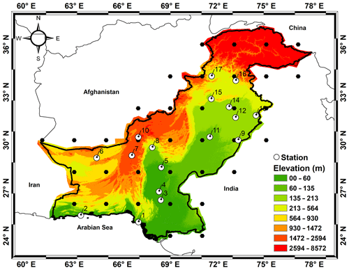
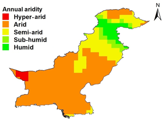
As shown in Fig. 1, Pakistan located in south Asia shares its border with India in the east, China in the north, Afghanistan and Iran in the west, and the Arabian Sea in the south. Pakistan has a rugged topography ranging from 0 m in the south to 8572 m in the north. Figure 2, which is based on the study by Ahmed et al. (2019d), shows that a large area of Pakistan experiences an arid climate, followed by a semi-arid climate, while a small area in the southwest region experiences a hyper-arid climate. However, a small area in the northernmost region of the country experiences a sub-humid to humid climate.

Pakistan receives summer monsoon precipitation during the period June–September and winter precipitation during the period December–March. Besides that, there are two intermediate rainy seasons called the pre-monsoon and the post-monsoon during the periods April–May and October–November, respectively (Sheikh, 2001). The bulk of the summer precipitation is caused by the monsoon winds that arise from the Bay of Bengal while westerly disturbances in the Mediterranean Sea are responsible for the winter precipitation. The average precipitation in Pakistan widely varies from southwest to northern parts in the range of <100 to >1000 mm yr⁻¹ (based on data from 1961 to 2010). Since the country is mostly characterized by arid and semi-arid climate, the bulk of the country receives precipitation of less than 500 mm yr⁻¹, while only a very limited area in the north receives more than 1000 mm yr⁻¹ of precipitation (Ahmed et al., 2017). The average temperature of the country varies from 0 ^∘C in the northern region to 32 ^∘C in the southern region (Khan et al., 2018b).

Figure 1 The location of Pakistan in central–south Asia and the GCM grid points over the country along with the locations of precipitation and temperature observation stations. The names of the stations are given in Table 2.

2.2 Datasets

2.2.1 Gridded precipitation and temperature data

The lack of long records of climate observations with extensive spatial coverage is a major issue in hydro-climatological investigations in many regions. As a solution to this problem, gridded datasets based on observations and various interpolation and data assimilation techniques have been created (Kishore et al., 2015). In this investigation, gridded monthly precipitation data of the Global Precipitation Climatology Center (GPCC) (Schneider et al., 2013) (https://dwd.de/EN/ourservices/gpcc/gpcc.html, last access: 3 May 2018) and gridded monthly maximum and minimum temperature data of the Climatic Research Unit (CRU) of East Anglia University (https://crudata.uea.ac.uk/cru/data/hrg/, last access: 3 May 2018) (Harris et al., 2014) were used as the surrogates of observed precipitation and maximum and minimum temperature respectively for the period 1961–2005. GPCC precipitation and CRU temperature data are available at a spatial resolution of 0.5^∘. As stated in the existing literature GPCC and CRU data are of high quality (Shiru et al., 2018; Salman et al., 2018b) and have an excellent seamless spatial and temporal coverage (Spinoni et al., 2014). Most importantly, GPCC precipitation and CRU temperature data have shown correlations above 0.80 with observed precipitation and maximum and minimum temperature over Pakistan (Ahmed et al., 2019c).

2.2.2 GCM precipitation and temperature data

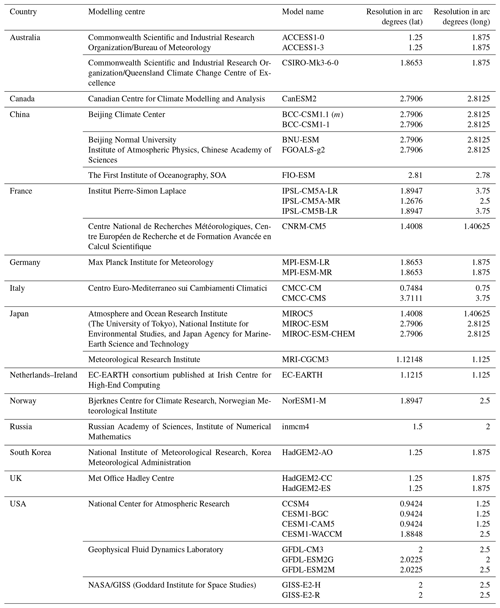
Monthly precipitation data simulated by the 36 CMIP5 GCMs for ensemble run r1i1p1 were extracted from the IPCC data distribution centre (http://www.ipcc-data.org/sim/gcm_monthly/AR5/Reference-Archive.html, last access: 10 April 2018) for the period 1961–2005. The modelling centres, names of GCMs and spatial resolution of each of the selected GCMs are provided in Table 1. In order to have a common spatial resolution, precipitation (P), maximum temperature (T_max), and minimum temperature (T_min) data obtained from different GCMs and GPCC and CRU databases were interpolated into a common $\mathrm{2}{}^{\circ }\times \mathrm{2}{}^{\circ }$ grid using bilinear interpolation.

Figure 2 Aridity classification of Pakistan (adopted from Ahmed et al., 2019d).

Table 1 CMIP5 GCMs considered in this study.

3 Methodology

In this study, GCMs for annual, monsoon, winter, pre-monsoon, and post-monsoon P, T_max, and T_min were first ranked separately (individual ranking) using six spatial performance measures; SPAEF, FSS, lambda, Cramer V, Mapcurves, and KGE. Then a comprehensive rating metric (RM) (Jiang et al., 2015) was used to rank the GCMs considering the individual ranks determined corresponding to all above spatial performance measures. The RM values of GCMs obtained for each variable were combined for deriving the overall ranks of GCMs. Finally, a sub-set of GCMs (MME) based on the overall ranks was selected and P, T_max, and T_min data for the MME were derived. The procedure used for the ranking, identification of the ensemble of GCMs and derivation of P, T_max, and T_min data from the multi-model ensemble of GCMs is outlined as follows.

1. All GCM-simulated P, T_max, and T_min data for the period 1961–2005 were remapped to a common grid with a $\mathrm{2}{}^{\circ }\times \mathrm{2}{}^{\circ }$ resolution.

2. SPAEF, FSS, lambda, Cramer V, Mapcurves, and KGE were individually applied to annual, monsoon, winter, pre-monsoon, and post-monsoon P, T_max, and T_min data for the period 1961–2005.

3. The goodness of fit (GOF) estimated by SPAEF, FSS, lambda, Cramer V, Mapcurves, and KGE for annual, monsoon, winter, pre-monsoon, and post-monsoon P, T_max, and T_min were used to rank the GCMs separately.

4. Comprehensive RMs were used to combine the ranks of GCMs determined by the above spatial performance measures separately for P, T_max, and T_min.

5. RMs were again used to derive the overall ranks of GCMs considering P, T_max, and T_min together for the entire study area.

6. The four top-ranked GCMs based on their overall ranks in replicating annual, monsoon, winter, pre-monsoon, and post-monsoon P, T_max, and T_min were identified.

7. Simple average and random forest techniques were used to generate MME P, T_max, and T_min means with the P, T_max, and T_min simulated by the four top-ranked GCMs identified in step 6.

8. Finally, the spatial patterns of MME P, T_max, and T_min generated using SM and RF were validated by visually comparing them with the spatial patterns of observed P, T_max, and T_min.

Details of the methods and the determination of the best-performing ensemble of GCMs are provided in the following sections.

3.1 Accuracy assessment of gridded precipitation and temperature data

The accuracy of gridded GPCC precipitation data and CRU temperature data was assessed by comparing them with the observed station data using normalized root mean square error (NRMSE) and modified index of agreement (md). NRMSE is a non-dimensional form of RMSE which is derived by normalizing RMSE by the range of observations. NRMSE is more reliable than RMSE in comparing model performance when the model outputs are in different units or the same unit but with different orders of magnitude (Willmott, 1982). NRMSE can have any positive value; however, values closer to 0 are preferred as they denote smaller errors (Chen and Liu, 2012). In this study, NRMSE was calculated using Eq. (1).

$$\begin{array}{}\text{(1)}& \mathrm{NRMSE}={\displaystyle \frac{{\left[\frac{\mathrm{1}}{N}{\sum }_{i=\mathrm{1}}^N{\left(x_{\mathrm{sim},i}-x_{\mathrm{obs},i}\right)}^{\mathrm{2}}\right]}^{\mathrm{1}/\mathrm{2}}}{x_{\max }-x_{\min }}}\end{array}$$

Here, x_sim,iand x_obs,i refer to the ith value in the gridded and observed time series of the climate variable (i.e. precipitation or temperature) respectively, and N is the number of data points in each time series.

The “md” shown in Eq. (2) is widely used to estimate the agreement between observed and gridded data of climate variables (Noor et al., 2019; Ahmed et al., 2019b). It varies between 0 (no agreement) and 1 (perfect agreement) (Willmott, 1981).

$$\begin{array}{}\text{(2)}& \mathrm{md}=\mathrm{1}-{\displaystyle \frac{{\sum }_{i=\mathrm{1}}^n{\left(x_{\mathrm{obs},i}-x_{\mathrm{sim},i}\right)}^j}{{\sum }_{i=\mathrm{1}}^n{\left(\left|x_{\mathrm{sim},i}-\stackrel{\mathrm{‾}}{x_{\mathrm{obs}}}\right|+\left|x_{\mathrm{obs},i}-\stackrel{\mathrm{‾}}{x_{\mathrm{obs}}}\right|\right)}^j}}\end{array}$$

Here, x_sim,i and x_obs,i are the ith value in the gridded data and observed data series of a climate variable.

3.2 GCM performance assessment

SPAEF, FSS, lambda, Cramer V, Mapcurves, and KGE were individually applied on each year from 1961 to 2005 of mean annual, monsoon, winter, pre-monsoon, and post-monsoon P, T_max, and T_min. Later, the GOF values of each year were temporally averaged to obtain a value for the entire study area. The details of the metrics are given below.

3.2.1 SPAtial EFficiency metric (SPAEF)

SPAEF, proposed by Demirel et al. (2018), is a robust spatial performance metric which considers three statistical measures, (1) Pearson correlation, (2) coefficient of variation, and (3) histogram overlap, in the assessment of the GOF of a model. The major advantage of SPAEF is that it combines the information derived from the above three independent statistical measures into one metric. The SPAEF values between past observed GPCC P, CRU T_max, and T_min and GCM-simulated P, T_max, and T_min were calculated using Eq. (3). In Eq. (3), α is the Pearson correlation coefficient between observed and GCM-simulated data, β is the spatial variability, and γ is the overlap between the histograms of observed and GCM-simulated data.

$$\begin{array}{}\text{(3)}& \mathrm{SPAEF}=\mathrm{1}-\sqrt{{\left(\mathit{\alpha }-\mathrm{1}\right)}^{\mathrm{2}}+{\left(\mathit{\beta }-\mathrm{1}\right)}^{\mathrm{2}}+{\left(\mathit{\gamma }-\mathrm{1}\right)}^{\mathrm{2}}}\end{array}$$

Equations (4) and (5) show the procedure for β and γ calculations respectively (for Pearson correlation (α) refer to Pearson, 1948). In Eq. (4) σ_G and σ_O refer to standard deviation of GCM-simulated and observed data respectively and μ_G and μ_O refer to the means of GCM-simulated and observed data respectively.

$$\begin{array}{}\text{(4)}& \mathit{\beta }={\displaystyle \frac{\left(\frac{{\mathit{\sigma }}_{\mathrm{G}}}{{\mathit{\mu }}_{\mathrm{G}}}\right)}{\left(\frac{{\mathit{\sigma }}_{\mathrm{O}}}{{\mathit{\mu }}_{\mathrm{O}}}\right)}}\end{array}$$

In Eq. (5), K, L, and n refer to histogram values of observations, histogram values of GCM simulations, and the number of bins in a histogram.

$$\begin{array}{}\text{(5)}& \mathit{\gamma }={\displaystyle \frac{{\sum }_{j=\mathrm{1}}^n\min (K_j,L_j)}{{\sum }_{j=\mathrm{1}}^n{K}_j}}\end{array}$$

The SPAEF can have a value between −∞ and 1, where a value closer to 1 indicates higher spatial similarity between the observations and model simulations (Koch et al., 2018). A code written in MATLAB environment was used for calculating SPAEF values (Demirel et al., 2018).

3.2.2 Fractions skill score (FSS)

The fractions skill score proposed by Roberts and Lean (2008) is another measure used for the assessment of spatial agreement between model simulations and observations. FSS varies between 0 and 1 where a value closer to 1 refers to a higher agreement between observed and simulated data. In this study, FSS between observed and GCM-simulated data was computed using Eq. (6).

$$\begin{array}{}\text{(6)}& \mathrm{FSS}=\mathrm{1}-{\displaystyle \frac{{\mathrm{MSE}}_{\left(n\right)}}{{\mathrm{MSE}}_{\left(n\right)\mathrm{ref}}}}\end{array}$$

In Eq. (6) MSE refers mean square error and is calculated using Eqs. (7) and (8).

$$\begin{array}{}\text{(7)}& {\mathrm{MSE}}_{\left(n\right)}={\displaystyle \frac{\mathrm{1}}{N_x{N}_y}}\sum _{i=\mathrm{1}}^{N_x}.\sum _{j=\mathrm{1}}^{N_y}{\left[O_{\left(n\right)i,j}-M_{\left(n\right)i,j}\right]}^{\mathrm{2}}\end{array}$$

$$\begin{array}{}\text{(8)}& {\mathrm{MSE}}_{\left(n\right)\mathrm{ref}}={\displaystyle \frac{\mathrm{1}}{N_x{N}_y}}\left[\sum _{i=\mathrm{1}}^{N_x}\sum _{j=\mathrm{1}}^{N_y}{O}_{\left(n\right)i,j}^{\mathrm{2}}+\sum _{i=\mathrm{1}}^{N_x}\sum _{j=\mathrm{1}}^{N_y}{M}_{\left(n\right)i,j}^{\mathrm{2}}\right]\end{array}$$

In Eqs. (7) and (8) N_x and N_y are the number of columns and rows in an observed or simulated map of a climate variable respectively, O and M are observed and simulated data fractions respectively. The “verification” package (Pocernich, 2006) written in R programming language was employed in this study for estimating FSS values.

3.2.3 Goodman–Kruskal's lambda

Goodman–Kruskal's lambda, also known as the lambda coefficient (λ), is used to measure the nominal or categorical association between categorical maps (Goodman and Kruskal, 1954). The lambda coefficient varies between 0 and 1, where a value closer to 1 refers to a higher similarity between the map of model simulations and that of observations of P, T_max, and T_min. The lambda coefficient was calculated using Eq. (9), where max_j is the number of classes (categories) in the observed and simulated maps, c_ij is a contingency matrix (describes the relationships between the data classes), i and j are the classes in observed and simulated maps respectively, and m represents the number of classes in the observed and simulated maps. In the present study, seven classes in the contingency matrix were used by following the study by Demirel et al. (2018). The “DescTools” package (Signorell, 2016) written in R programming language was employed in this study for estimating the nominal and categorical association between observed and simulated maps.

$$\begin{array}{}\text{(9)}& \mathit{\lambda }={\displaystyle \frac{{\sum }_{i=\mathrm{1}}^m{\max }_j{c}_{ij}-{\max }_j{\sum }_{i=\mathrm{1}}^m{c}_{ij}}{N-{\max }_j{\sum }_{i=\mathrm{1}}^m{c}_{ij}}}\end{array}$$

3.2.4 Cramer's V

Cramer's V (Cramér, 1999) statistic is a chi-square-test-based measure which is used in assessing spatial agreement between observations and model simulations (Zawadzka et al., 2015). Its value ranges between 0 and 1 and value closer to 1 refers to a better agreement between the simulated and observed maps of the climate variable. Cramer's V was calculated using Eq. (10).

$$\begin{array}{}\text{(10)}& V=\sqrt{{\displaystyle \frac{x^{\mathrm{2}}}{N(min\left(m,n\right)-\mathrm{1}}}}\end{array}$$

Here, x² is chi-square, N is the grand total of observations, m is the number of rows and n is the number of columns. In this exercise m=42 (number of rows of data) and n=2 (observed and modelled precipitation). The “DescTools” package (Signorell, 2016) written in R programming language was employed in this study for calculating Cramer's V values.

3.2.5 Mapcurves

Mapcurves is another statistical measure, developed by Hargrove et al. (2006) for the measurement of similarity between categorical maps. Mapcurves quantifies the degree of concordance between two maps. The value of Mapcurves can vary from 0 to 1 (perfect agreement). In the present study, the degree of concordance between the historical observed P, T_max, and T_min maps and each of the GCM-simulated P, T_max, and T_min maps was determined using Eq. (11), where MC_X refers to the Mapcurves value, A is the total area of a given class X on the map being compared, B is the total area of a given class Y on the observed map, C is the area of intersection between X and Y when the maps are overlaid, and n is the number of classes in the observed map.

$$\begin{array}{}\text{(11)}& {\mathrm{MC}}_X=\sum _{Y=\mathrm{1}}^n\left[\left({\displaystyle \frac{C}{A}}\cdot {\displaystyle \frac{C}{B}}\right)\right]\end{array}$$

In this study, the function “mapcurves (x, y)” available in the “sabre” package (Nowosad and Stepinski, 2018) written in R programming language was used for estimating mapcurves values. In that equation x and y are vectors representing the categorical values of historical observed data (e.g. GPCC precipitation) and categorical values of simulated data by a GCM, respectively.

3.2.6 Kling–Gupta efficiency (KGE)

The Kling–Gupta efficiency is a GOF test developed by Gupta et al. (2009), for the model performance assessment. KGE considers three statistical measures, (1) Pearson correlation, (2) variability ratio, and (3) bias ratio, in the assessment of model performance. In the present study, KGE was calculated between historical observed data and GCM-simulated data using Eq. (12). KGE values can range between −∞ and 1, where values close to 1 are preferred.

$$\begin{array}{}\text{(12)}& \mathrm{KGE}=\mathrm{1}-\sqrt{{\left({\mathit{\alpha }}_{\mathrm{P}}-\mathrm{1}\right)}^{\mathrm{2}}+{\left({\mathit{\beta }}_{\mathrm{P}}-\mathrm{1}\right)}^{\mathrm{2}}+{\left({\mathit{\gamma }}_{\mathrm{RP}}-\mathrm{1}\right)}^{\mathrm{2}}}\end{array}$$

In Eq. (12), α_P is the Pearson correlation (Pearson, 1948) between observed and GCM-simulated data, β_P is the bias ratio, and γ_RP is the variability ratio. Equations (13) and (14) show the calculation of β_P and γ_RP respectively.

$$\begin{array}{}\text{(13)}& {\mathit{\beta }}_{\mathrm{P}}={\displaystyle \frac{{\mathit{\mu }}_{\mathrm{G}}}{{\mathit{\mu }}_{\mathrm{O}}}}\end{array}$$

In Eq. (13), μ_G and μ_O refer to mean of GCM-simulated and observed data respectively.

$$\begin{array}{}\text{(14)}& {\mathit{\gamma }}_{\mathrm{RP}}={\displaystyle \frac{{\mathrm{CV}}_{\mathrm{G}}}{{\mathrm{CV}}_{\mathrm{O}}}}={\displaystyle \frac{\left(\frac{{\mathit{\sigma }}_{\mathrm{G}}}{{\mathit{\mu }}_{\mathrm{G}}}\right)}{\left(\frac{{\mathit{\sigma }}_{\mathrm{O}}}{{\mathit{\mu }}_{\mathrm{O}}}\right)}}\end{array}$$

In Eq. 14, CV_G and CV_O refer to the coefficient of variation of GCM-simulated and observed data respectively.

3.3 Comprehensive rating metrics

The ranking of GCMs with respect to a given climate variable using one single GOF measure is a relatively simple task. However, the ranking of GCMs becomes more challenging when multiple GOF measures are used with multiple climate variables, as different GCMs may display different degrees of accuracy for different GOF measures and climate variables. In such a case, an information aggregation approach that combines information from several GOF measures can be used. In this study, a comprehensive rating metric (Chen et al., 2011) was used to obtain the overall ranks of GCMs. The overall ranks of GCMs based on different GOFs were obtained for each season separately using Eq. (15).

$$\begin{array}{}\text{(15)}& \mathrm{RM}=\mathrm{1}-{\displaystyle \frac{\mathrm{1}}{\mathrm{nm}}}\sum _{i=\mathrm{1}}^n{\mathrm{rank}}_i\end{array}$$

In Eq. (15), n refers to the number of GCMs, m refers to the number of metrics or seasons and i refers to the rank of a GCM based on the ith GOF. A value of RM near to 1 refers to a better GCM in terms of its ability to mimic the spatial or temporal characteristics of observations.

3.4 Identification of ensemble members

The uncertainties in climate projections which arise from GCM structure, assumptions and approximations, initial conditions, and parameterization can be reduced by identifying an ensemble of better-performing GCMs (Kim et al., 2015). Lutz et al. (2016) reported that one or a small ensemble of GCMs is suitable for climate change impact assessment. A number of studies (Weigel et al., 2010; Miao et al., 2012) have suggested that one GCM is not enough to assess the uncertainties associated with the future climate. Therefore, identification of an ensemble of GCMs is a necessity in climate change impact assessments. In the present study, four top-ranked GCMs were considered for the development of MMEs for P, T_max, and T_min. The review of the literature revealed that there is no well-defined guideline on the selection of the optimum number of GCMs for the MME, and most of the studies considered the first 3 to 10 GCMs ranked according to the descending order of their performance for the MME. For instance, in the study by Xuan et al. (2017) over Zhejiang, China, 10 top-ranked GCMs for an MME for precipitation were used. In another study over China, Jiang et al. (2015) developed MMEs for daily temperature extremes using the five top-ranked GCMs. In a study over Pakistan, Khan et al. (2018a) considered six common GCMs that appeared in the lists of 10 top-ranked GCMs for daily temperature and precipitation. Ahmadalipour et al. (2017) used the four top-ranked GCMs for simulating daily precipitation and temperature over the Columbia River Basin in the Pacific Northwest USA. In the study by Hussain et al. (2018) the three top-ranked GCMs for the development of an MME for precipitation over Bornean tropical rainforests in Malaysia were used.

In the present study, the ensemble of GCMs was identified in two steps: (1) RM values of GCMs for annual, monsoon, winter, pre-monsoon, and post-monsoon P, T_max, and T_min were individually used to derive an overall rank for each GCM, and (2) four top-ranked GCMs based on RM values for all climate variables were considered for the ensemble. The selection of an appropriate set of GCMs considering their skills in different seasons enables the selection of an ensemble which can better simulate the observations in different seasons.

3.5 Development of multi-model ensemble mean

The uncertainties in projections of a climate variable can be reduced by using its mean time series calculated from an MME of better-performing GCMs (You et al., 2018). Numerous approaches are documented in the literature for the calculation of mean time series from an ensemble of better-performing GCMs starting from simple arithmetic mean to machine learning algorithms (Kim et al., 2015). In the present study, two approaches, simple mean and random forest (Breiman, 2001), were used for the calculation of mean time series of P, T_max, and T_min corresponding to an ensemble of four top-ranked GCMs.

3.5.1 Simple mean (SM)

Simple-mean-based MMEs were developed by simply averaging the individual P, T_max, and T_min simulations of the four top-ranked GCMs using Eq. (16).

$$\begin{array}{}\text{(16)}& \mathrm{SM}={\displaystyle \frac{\mathrm{1}}{n}}\sum _{i=\mathrm{1}}^n{\mathrm{GCM}}_{\mathrm{i}}\end{array}$$

In Eq. (16), n refers to the number of GCMs considered for the development of MMEs, which is four in the present study, and GCM_i refers to the simulations of the climate variable of interest (i.e. P, T_max, and T_min) produced by the ith GCM.

Table 2 Validation of accuracy of GPCC P and CRU T_max and T_min using NRMSE and md.

3.5.2 Random forest (RF)

The random forest algorithm (Breiman, 2001) was used in the calculation of the mean time series of P, T_max, and T_min corresponding to an MME of four top-ranked GCMs. RF is a relatively new machine learning algorithm widely used in modelling non-linear relationships between predictors and predictands (Ahmed et al., 2019b). The RF algorithm is found to perform well with spatial datasets and is less prone to over-fitting (Folberth et al., 2019). Most importantly Folberth et al. (2019) reported that RF is less sensitive to multivariate correlation. RF is an ensemble technique where regression is done using multiple decision trees. RF algorithm uses the following steps in developing regression models.

1. A bootstrap resampling method is used to select sample sets from training data (i.e. GCM and observed data).

2. The classification and regression tree (CART) technique is used to develop unpruned trees using the bootstrapped samples.

3. A large number of trees are developed with the samples selected repetitively from training data so that all training data have an equal probability of selection.

4. A regression model is fitted to each tree and the performance of each tree is assessed.

5. Ensemble simulation is estimated by averaging the predictions of all trees, which is considered as the final simulation.

Wang et al. (2018) and He et al. (2016) reported that the performance of RF varies with the number of trees (n_tree) and the number of variables randomly sampled (m_try) at each split in developing the trees. In those studies, it was observed that RF performance increases with the increase in the value of ntree. However, in the current study the performance was not found to increase significantly in term of root mean square error when the value of ntree was greater than 500. Therefore, ntree was set to 500 while mtry was set to p∕3, where p is the number of variables (i.e. 4 GCMs) used for developing RF-based MME.

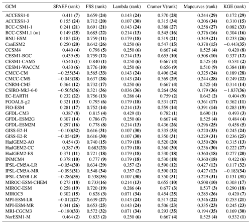
Table 3 GOF values and ranks of GCMs obtained using different spatial metrics for mean annual precipitation. Bold numbers within brackets represent the rank of GCMs.

The MME prediction can be improved by assigning larger weights to the GCMs which show better performance (Sa'adi et al., 2017). RF regression models developed using historical P, T_max, and T_min simulations of GCMs as independent variables and historical observed P, T_max, and T_min as dependent variables provide weights to the GCMs according to their ability to simulate historical observed P, T_max, and T_min. The “randomForest” package (Breiman, 2006) written in R programming language was employed in this study for developing RF-based MMEs. RF-based MMEs were calibrated with the first 70 % of the data and validated with the rest of the data.

4 Results and discussion

4.1 Accuracy assessment of gridded precipitation data

As a preliminary analysis, the monthly time series of GPCC P, CRU T_max, and CRU T_min data were validated against the monthly time series of observed P,T_max, and T_min. The validation was performed for the period 1961–2005. In the present study, two statistical metrics, normalized root mean square error (NRMSE) and modified index of agreement (md), were used to assess the accuracy of monthly time series of GPCC P, CRU T_max, and CRU T_min in replicating the mean and the variability of monthly time series of observed P,T_max, and T_min.

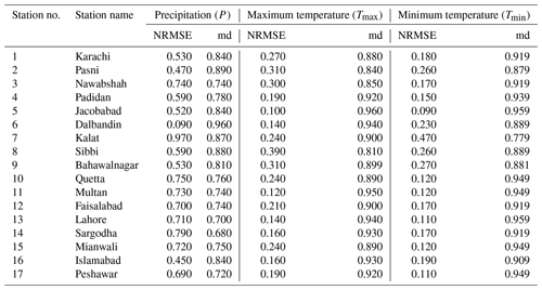
The NRMSE and md values between observed P and GPCC P (pertaining to the grid point closest to the observation station) and between observed T_max and T_min with CRU T_max and T_min obtained for 17 locations in Pakistan are given in Table 2. Overall, all the stations showed low and high NRMSE and md values respectively, indicating that the accuracy of the GPCC P in replicating observed precipitation and CRU T_max and CRU T_min in replicating observed T_max and T_min over Pakistan is high. Overall, NRMSE values were found in the ranges of 0.09 to 0.970 for P, 0.100 to 0.390 for T_max, and 0.09 to 0.470 for T_min. Overall, md values were found in the ranges of 0.680 to 0.960 for P, 0.810 to 0.960 for T_max, and 0.779 to 0.959 for T_min.

Table 4 Ranks of GCMs for P, T_max, and T_min based on rating metric values.

4.2 Evaluation and ranking of GCMs

SPAEF, FSS, lambda, Cramer V, Mapcurves, and KGE between observed (GPCC P, CRU T_max, and T_min) and GCM-simulated mean annual, monsoon, winter, pre-monsoon, and post-monsoon P, T_max, and T_min in Pakistan were estimated for the period 1961 to 2005. As an example, Table 3 shows the GOF values that depict the performance of each GCM in simulating GPCC mean annual precipitation. In Table 3, the ranks of GCMs corresponding to each performance metric are shown within brackets. GOF values near to 1 refer to the better performance of the GCM of interest. For example, CESM1-CAM5 has a GOF value of 0.540 for SPAEF and is hence regarded as the best GCM in term of SPAEF, whereas CSIRO-Mk3-6-0 can be regarded as the poorest GCM, which has a GOF value of −0.505 in terms of SPAEF. The GOF values for other metrics (i.e. FSS, lambda, Cramer V, Mapcurves, and KGE) can also be interpreted in the same manner.

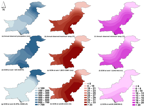
Figure 3 Spatial patterns of (a) GPCC precipitation, (b) CRU maximum temperature, (c) CRU minimum temperature, (d–f) GCM ranked 1, and (g–i) GCM ranked 36 for mean annual precipitation and maximum and minimum temperature for the period 1961 to 2005.

Table 5 Overall ranks of GCMs for the identification of ensemble members. Bold numbers represent the selected GCMs.

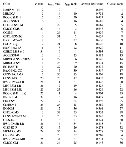
Table 3 shows the ranks attained by GCMs corresponding to different metrics. For example, BCC-CSM1.1 (m) attained ranks 25, 22, 13, 16, 16, and 16 in terms of SPAEF, FSS, lambda, Cramer V, Mapcurves, and KGE respectively. It was observed that CSIRO-Mk3-6-0 is the only GCM which was able to secure the same rank for all metrics. However, HadGEM2-ES secured rank 18 for four metrics (i.e. FSS, lambda, Cramer V, Mapcurves). Several GCMs attained the same rank for three metrics (e.g. BCC-CSM1.1 (m), CCSM4, CMCC-CM, and CMCC-CMS). Cramer V and Mapcurve showed more or less similar ranks for GCMs. Similar results were also seen for other seasons and variables (not presented in this paper).

4.3 Overall ranks of GCMs for precipitation, maximum temperature, and minimum temperature

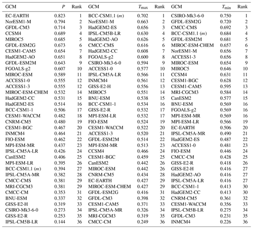
The application of various evaluation metrics has yielded different ranks for the same GCM (Ahmadalipour et al., 2017; Raju et al., 2017). The ranks attained by GCMs corresponding to different metrics and seasons (annual, monsoon, winter, pre-monsoon, and post-monsoon) were used to calculate the RM values for each GCM. The ranks of GCMs for P, T_max, and T_min are presented in Table 4 along with the RM values. As seen in Table 4, EC-EARTH, BCC-CSM1.1 (m), and CSIRO-Mk3-6-0 were the most skilful GCMs in reproducing the spatial characteristics of P, T_max, and T_min respectively. On the other hand, IPSL-CM5B-LR, CMCC-CM, and INMCM4 were poorest GCMs in reproducing the spatial characteristics of P, T_max, and T_min respectively.

The better performance of EC-EARTH, BCC-CSM1.1 (m), and CSIRO-Mk3-6-0 in simulating P, T_max, and T_min over south Asia has also been reported in several past studies. Latif et al. (2018) reported the relatively better performance of EC-EARTH and BCC-CSM1.1 (m) out of 36 CMIP5 GCMs in simulating precipitation over south Asia based on spatial correlations. Rehman et al. (2018) conducted a study to assess the performance of CMIP5 GCMs in simulating mean precipitation and temperature over south Asia. The study reported the better performance of EC-EARTH in simulating precipitation and CSIRO-Mk3-6-0 in simulating temperature. Khan et al. (2018a) assessed the performance of 31 CMIP5 GCMs in simulating mean precipitation and temperature over Pakistan using multiple daily gridded datasets and identified EC-EARTH as the best GCM for simulating precipitation and CSIRO-Mk3-6-0 for simulating temperature. A better performance of CSIRO-Mk3-6-0 in simulating maximum and minimum temperature is also reported in the study by Ahmed et al. (2019c).

The spatial patterns of mean annual P, T_max, and T_min simulated by the GCMs ranked 1 and 36 were compared with the spatial patterns of GPCC P and CRU T_max and T_min and presented in Fig. 3 as an example. In Fig. 3 it was seen that the GCMs that attained rank 1 (the best-performing GCM) showed spatial patterns more or less similar to those of GPCC P and CRU T_max and T_min. On the other hand, GCMs ranked 36 (the worst-performing GCM) showed large differences compared to the spatial patterns of GPCC P and CRU T_max and T_min. Figure 3 clearly shows that GCMs which attained rank 36 underestimated the precipitation and temperature over a large region in the study area.

4.4 Identification of ensemble members

Based on the criteria mentioned in Section 3.4, ranks of each variable were estimated and then the GCMs were ranked based on the overall RM values. Table 5 shows the overall ranks of the 36 GCMs considered in this study. The four top-ranked GCMs (NorESM1-M, MIROC5, BCC-CSM1-1, and ACCESS1-3, which are indicated in bold text in Table 5) were selected as the members of the ensemble for P, T_max, and T_min over Pakistan.

The performances of the four top-ranked GCMs (i.e. GCMs ranked 1, 2, 3, and 4) and four lowest-ranked GCMs (i.e. GCMs ranked 33, 34, 35, and 36) were visually evaluated using scatter plots shown in Figs. 4 and 5, pertaining to mean annual P, T_max, and T_min as an example. In order to plot the scatter, the P, T_max, and T_min simulated by each GCM and GPCC P, CRU T_max, and CRU T_min pertaining to all grid points were averaged (spatially averaged precipitation and temperature). As expected, GCMs that attained ranks 1 to 4 showed a close agreement with the GPCC P, CRU T_max, and CRU T_min compared to GCMs which attained ranks 33, 34, 35, and 36. The same can also be noticed based on md values provided in each figure where top-ranked GCMs showed higher md values compared to the lowest-ranked GCMs. The scatter plots in Fig. 5 indicated that the least skilful GCMs underestimated mean annual P, T_max, and T_min. Over- and underestimation of P, T_max, and T_min can also be seen in the scatter plots of GCMs ranked 1, 2, 3, and 4. However, their scatter was found to be much aligned with the 45^∘ line compared to that of GCMs ranked 33, 34, 35, and 36. Therefore, it is argued that the GCMs ranked 1, 2, 3 and 4 can be used as an ensemble for the simulation of P, T_max, and T_min.

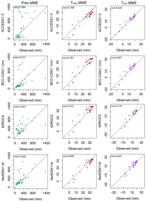
Figure 4 Scatter of spatially averaged annual P, T_max and T_min of four top-ranked GCMs plotted against GPCC P, CRU T_max, and CRU T_min for the period 1961 to 2005.

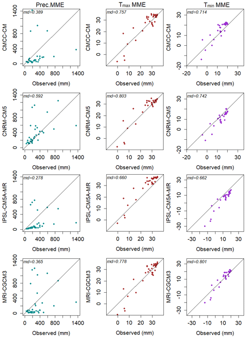
Figure 5 Scatter of spatially averaged annual P, T_max, and T_min of four lowest ranked GCMs plotted against GPCC P, CRU T_max, and CRU T_min for the period 1961 to 2005.

Some of the GCMs identified for the ensemble over Pakistan in this study have also been identified as better-performing GCMs over neighbouring countries such as India and Iran. Jena et al. (2015) used Z-value test, correlation coefficient, relative precipitation comparison test, probability function comparison, root mean square error, and Student's t test to evaluate the performance of 20 CMIP5 GCMs in simulating the Indian summer monsoon. They found that CCSM4, CESM1-CAM5, GFDL-CM3, and GFDL-ESM2G perform better compared to the other GCMs. Prasanna (2015) conducted a study to assess the performance of 12 CMIP5 GCMs using mean and coefficient of variation over south Asia (5–35^∘ N; 65–95^∘ E) and identified ACCESS, CNRM, HadGEM2-ES, MIROC5, Can-ESM, GFDL-ESM2M, GISS, MPI-ESM, and NOR-ESM as better-performing GCMs. Sarthi et al. (2016) evaluated the performance of 34 CMIP5 GCMs using the Taylor diagram, skill score, correlation, and RMSE. They found that BCC-CSM1.1 (m), CCSM4, CESM1(BGC), CESM1(CAM5), CESM1(WACCM), and MPI-ESM-MR were able to better capture the Indian summer monsoon precipitation. Afshar et al. (2016) applied the Nash–Sutcliffe efficiency, percent of bias, coefficient of determination, and the ratio of RMSE to standard deviation of observations for assessing the performance of precipitation simulations of 14 CMIP5 GCMs over a mountainous catchment in north-eastern Iran, which borders Pakistan. They recommend GFDL-ESM2G, IPSL-CM5A-MR, MIROC-ESM, and NorESM1-M as better GCMs. Mahmood et al. (2018) used the correlation coefficient, error between observed and GCM mean and standard deviation, and root mean square error to assess the performance of CMIP5 GCMs in simulating precipitation over Jhelum river basin, Pakistan, and reported the good performance of GFDL-ESM2G, HadGEM2-ES, NorESM1-ME, CanESM2, and MIROC5. Latif et al. (2018) reported better performance of HadGEM2-AO, INM-CM4, CNRM-CM5, NorESM1-M, CCSM4, and CESM1-WACCM out of 36 GCMs in simulating precipitation over the Indo-Pakistan region based on partial correlation. The above findings indicated that the GCMs identified in this study for the ensemble were also found to perform well in the other studies conducted over nearby countries and regions.

Figure 6 Spatial patterns of (a) GPCC precipitation, (b) CRU maximum temperature, (c) CRU minimum temperature, (d–f) MME-based on simple mean (SM), and (g–i) MME-based on the random forest (RF) algorithm for mean annual precipitation and maximum and minimum temperature for the period 1961 to 2005.

4.5 Multi-model ensemble (MME) mean

The performance of GCM ensembles identified in Section 4.4 was validated considering two types of MME means. The MME mean of P,T_max, and T_min of the four top-ranked GCMs was calculated with SM and RF. In the application of SM, the time series of P,T_max, and T_min of the four top-ranked GCMs were averaged to obtain the MME while in the application of RF, the time series of P,T_max, and T_min of the four top-ranked GCMs were considered as inputs to the RF-based MME.

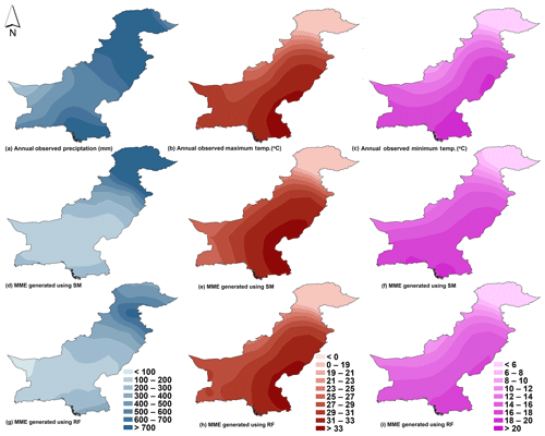
In Fig. 6, the spatial patterns of P,T_max, and T_min corresponding to both MMEs derived with SM and RF were compared with those of GPCC P, CRU T_max, and CRU T_min. The spatial patterns of P,T_max, and T_min were created using ordinary kriging technique. Ordinary kriging was selected as it was found to perform better than other interpolation methods over Pakistan (Ahmed et al., 2014). As seen in Fig. 6, both MMEs captured the spatial patterns of observed P,T_max, and T_min to a good degree. However, the differences can be seen in both MMEs in replicating the spatial pattern of GPCC P, CRU T_max, and CRU T_min. The visual comparison provided in Fig. 6 also indicated that RF-based MME performs better than the MME based on SM. SM-based MME was found to underestimate annual precipitation in the south-western and the northern regions, while the RF-based MME was found to produce a spatial pattern almost identical to that of GPCC precipitation. A similar result can also be seen for T_max, and T_min patterns where RF-based MME showed better performance. The better performance of RF in generating MMEs has also been reported in several other studies. Salman et al. (2018a) generated the MME mean for maximum and minimum temperature over Iraq using four CMIP5 GCMs and reported that RF-based MME performed better compared to individual GCMs. Likewise, Wang et al. (2018) conducted a comprehensive study to evaluate the performance of different machine learning techniques including RF, a support vector machine, Bayesian model averaging, and the arithmetic ensemble mean in generating MMEs. They considered 33 CMIP5 GCMs for precipitation and temperature over 108 stations located in Australia and concluded that RF and SVM can generate better-performing MMEs compared to other techniques.

The performance of MME ensembles was further evaluated using scatter plots shown in Fig. 7. Scatter plots were developed using spatially averaged GPCC P, CRU T_max, and CRU T_min and MME annual P, T_max, and T_min at all grid points for the period 1961–2005. According to scatter plots in Fig. 7, RF-based MME performed significantly better compared to its counterpart SM-based MME in simulating P,T_max, and T_min.

In this study performance of GCMs was assessed based on their ability to simulate past observed P, T_max, and T_min and hence the best-performing GCMs were identified and used for the development of MMEs. However, it is found that past and future climate may have a weak association and hence it is not guaranteed that a GCM that performed well in the past will produce reliable results in future (Knutti et al., 2010). In other words, the best GCMs selected for the MMEs considering their ability to simulate past climate may not be the best in the future under changing climate (Ruane and McDermid, 2017; Ahmed et al., 2019c). This is due to the large uncertainties associated with GHG emission scenarios and GCMs. As a solution to this limitation, Salman et al. (2018a) selected an ensemble of GCMs based on past performance as well as the degree of agreement between their future projections. The study detailed in the present paper can be repeated in future to select GCMs considering their past performance and the degree of agreement in their future projections.

In the present study, the MMEs of P, T_max, and T_min were developed by considering four top-ranked GCMs. In the past, MMEs were developed considering 3 to 10 top-ranked GCMs. However, none of the past studies investigated the performance of MMEs by varying the number of GCMs used in developing them in MME. The performance of an MME can be sensitive to the choice of the number of GCMs. Hence, in future, a study should be conducted to investigate the impact of the number of GCMs used for the development of the MME.

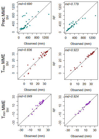
Figure 7 Scatter of spatially averaged annual P, T_max and T_min of MMEs developed with simple mean (SM) and random forest (RF) using four top-ranked GCMs plotted against GPCC P, CRU T_max, and CRU T_min for the period 1961 to 2005.

Only the RF algorithm was used in this study for the development of MMEs. Other machine learning algorithms (e.g. artificial neural networks, support vector machine, relevance vector machine, k-nearest neighbour, extreme learning machine) can also be used for the development of MMEs. A comparison of the performance of MMEs developed with different machine learning algorithms can assist in the identification of the pros and cons of different algorithms in relation to the development of MMEs.

In the present study, GCM ranking and MME development was conducted only considering P, T_max, and T_min pertaining to annual, monsoon, winter, pre-monsoon, and post-monsoon seasons. However, several studies reported that the ranking of GCMs based on a variety of climate variables may assist in the identification of a more dependable set of GCMs for an MME (Johnson and Sharma, 2012; Xuan et al., 2017). In future, the ranking of GCMs can be conducted considering a number of climate variables such as precipitation, mean temperature, maximum temperature, minimum temperature, wind speed, evapotranspiration, and solar radiation.

5 Conclusions

This study quantitatively and qualitatively assessed the spatial accuracy of 36 CMIP5 GCMs in simulating annual, monsoon, winter, pre-monsoon, and post-monsoon precipitation and maximum and minimum temperature over Pakistan for the period 1961–2005. The quantitative evaluation was conducted using six state-of-the-art spatial metrics (SPAtial EFficiency, fractions skill score, Goodman–Kruskal's lambda, Cramer's V, Mapcurves, and Kling–Gupta efficiency), and qualitative evaluation was done using scatter plots. A comprehensive rating metric was used to derive the overall ranks of GCMs based on their ranks pertaining to annual, monsoon, winter, pre-monsoon, and post-monsoon precipitation and maximum and minimum temperature.

Following conclusions were drawn from this study:

1. The low normalized root mean square error (NRMSE) and high modified index of agreement (md) confirmed the close agreement of monthly Global Precipitation Climatology Center (GPCC) precipitation and Climatic Research Unit (CRU) temperature with the observed precipitation and temperature extracted from 17 stations located in different climate zones in Pakistan. The low NRMSE and high md values of GPCC precipitation and CRU temperature can be associated with extensive data quality control measures and the use of a large number of stations for the development of GPCC precipitation and CRU temperature datasets (Schneider et al., 2013; Harris et al., 2014).

2. Ranks of the 36 GCMs derived based on all spatial metrics (SPAtial EFficiency, fractions skill score, Goodman–Kruskal's lambda, Cramer's V, Mapcurves, and Kling–Gupta efficiency) for the period 1961–2005 were found mostly similar to each other during a given season (i.e. annual, monsoon, winter, pre-monsoon, and post-monsoon) for a given climate variable (i.e. precipitation and maximum and minimum temperature). However, it was noticed that different GCMs performed significantly differently in simulating different variables (i.e. precipitation and maximum and minimum temperature).

3. EC-EARTH, BCC-CSM1.1 (m), and CSIRO-Mk3-6-0 were identified as the most skilful GCMs while IPSL-CM5B-LR, CMCC-CM, and INMCM4 were identified as the least skilful GCMs in simulating precipitation, maximum temperature and minimum temperature over Pakistan, respectively. The overall ranks of GCMs based on a comprehensive rating metric revealed that NorESM1-M, MIROC5, BCC-CSM1-1, and ACCESS1-3 are the most suitable GCMs for simulating all three climate variables (i.e. precipitation and maximum and minimum temperature) over Pakistan.

4. The spatial patterns of precipitation and maximum and minimum temperature of four top-ranked GCMs and their MME mean precipitation and maximum and minimum temperature generated using simple mean (SM) and random forest (RF) techniques for annual, monsoon, winter, pre-monsoon, and post-monsoon seasons showed more or less similar spatial patterns to those of GPCC precipitation and CRU maximum and minimum temperature. Moreover, the comparison of MME mean precipitation and maximum and minimum temperature corresponding to annual, monsoon, winter, pre-monsoon, and post-monsoon seasons generated using SM and RF techniques clearly showed the superiority of RF in replicating the spatial patterns of the GPCC precipitation and CRU maximum and minimum temperature.