Comparison of approaches to interpolating climate observations in steep terrain with low-density gauging networks

The accuracy of hydrological assessments in mountain regions is often hindered by the low density of gauges coupled with complex spatial variations in climate. Increasingly, spatial datasets (i.e. satellite and other products) and new computational tools are merged with ground observations to address this problem. This paper presents a comparison of approaches of different complexities to spatially interpolate monthly precipitation and daily temperature time series in the upper Aconcagua catchment in central Chile. A generalised linear mixed model (GLMM) whose parameters are estimated through approximate Bayesian inference is compared with simpler alternatives: inverse distance weighting (IDW), lapse rates (LRs), and two methods that analyse the residuals between observations and WorldClim (WC) data or Climate Hazards Group Infrared Precipitation with Station data (CHIRPS). The assessment is based on a leave-one-out cross validation (LOOCV), with the root-mean-squared error (RMSE) being the primary performance criterion for both climate variables, while the probability of detection (POD) and false-alarm ratio (FAR) are also used for precipitation. Results show that for spatial interpolation of temperature and precipitation, the approaches based on the WorldClim or CHIRPS residuals may be recommended as being more accurate, easy to apply and relatively robust to tested reductions in the number of estimation gauges. The GLMM has comparable performance when all gauges were included and is better for estimating occurrence of precipitation but is more sensitive to the reduction in the number of gauges used for estimation, which is a constraint in sparsely monitored catchments.

1 Introduction

Climate variables such as temperature and precipitation are key inputs for hydrological modelling and water resource management. Generally, spatial interpolation of point observations is a necessary part of developing the climate inputs of models. Many interpolation approaches perform well for gentle terrain; however, their accuracy and precision decrease in mountain areas (Wu and Li, 2013; Frei, 2014; Buytaert et al., 2006). As highlighted by Dorninger et al. (2008), challenges include observation errors, anisotropic climate patterns, and sensitivity of results to density and location of observations. Strongly non-linear relations between temperature and altitude may be related to physiographic features (Stahl et al., 2006), to cold air trapped in enclosing hill ranges (Frei, 2014) and also to the presence of glaciers (Ragettli et al., 2014). For precipitation, non-linearity can be related to physiographic features (Daly et al., 2008), to the interaction between topography and rainstorms (Falvey and Garreaud, 2007; Garreaud, 2013), and to summertime convective precipitation events (Viale and Garreaud, 2014).

The Andes Cordillera in South America is an example of a steep terrain with complex weather conditions. This mountain range is an important source of natural resources, including water for agriculture, mining and other industries. The streamflows in the region are highly variable in both time and space (Pellicciotti et al., 2007; Mernild et al., 2017; Montecinos and Aceituno, 2003; Viale and Garreaud, 2014); therefore under such circumstances, quality of spatial climate data is a key issue when modelling water resources (Zambrano-Bigiarini et al., 2016; Mernild et al., 2017). This challenge is further complicated by the lack of gauges (i.e. when compared to mountain regions in Europe or North America), particularly at high-elevation points. As a consequence, several hydrological and water resources models in some regions of the Andes, such as central Chile, have applied deterministic interpolation approaches such as lapse rates (LRs; Ragettli and Pellicciotti, 2012; Ragettli et al., 2014; Vicuña et al., 2011; Stehr et al., 2008; Correa-Ibanez et al., 2017) to define climate inputs. Although easy to apply, the LR in hydrological applications is usually a linear or logarithmic regression using elevation as the only covariate (Ragettli and Pellicciotti, 2012) and hence does not aim to maintain the spatial correlation between observations or to fully explore the spatial dynamics of the climate variables. Therefore, there is an increasing interest in the use of improved interpolation approaches together with alternative sources of data, beyond point observations, such as satellites and other gridded products (Manz et al., 2016; Zambrano-Bigiarini et al., 2016; Dinku et al., 2010; Hobouchian et al., 2017; Demaria et al., 2013).

In the Andes, Álvarez‐Villa et al. (2011) tested four stochastic interpolation approaches in Colombia and found that the kriging with external drift (KED – using long-term averages of the Tropical Rainfall Measuring Mission – TRMM – as the drift term) approach had the best performance, with root-mean-squared errors (RMSEs) between 519 and 866 mm; however that analysis was restricted to annual precipitation estimates. In Castro et al. (2014) the authors developed a deterministic method that separated the analysis of occurrence and magnitude of events and that took into account the influence of topography (i.e. slope orientation and wind direction) to interpolate daily precipitation values in a catchment in central Chile and found that this method outperformed inverse distance weighting (IDW) and other simple methods. That analysis was restricted to gauges below 1000 m a.s.l.; thus conclusions may not be valid for higher-elevation points. This is a common limitation in the southern Andes, where there are few gauges above this elevation.

In Manz et al. (2016) the authors analysed a database of 735 gauges in Bolivia, Peru, Colombia and Ecuador (including 455 gauges above 1000 m a.s.l. in the tropical Andes) and merged them with the Tropical Rainfall Measuring Mission precipitation radar product (TRMM 2A25). The authors used deterministic (including IDW of residuals between monthly precipitation observations and satellite estimates) and kriging methods (including KED using mean monthly TRMM 2A25 values as the external drift term). It was found that for that case study, KED had the best performance amongst the kriging methods, that the overall performance of kriging methods was similar to the interpolation of residuals to estimate monthly precipitation values and that this interpolation of residuals was less sensitive to low gauge densities. In that study performance was assessed using leave-one-out cross validation (LOOCV) of the gauges, using metrics such as RMSE and runoff ratios.

A broader review of the performance of satellite products for estimating precipitation in the Andes and other mountain areas (Nikolopoulos et al., 2013; Thiemig et al., 2012; Dinku et al., 2014) suggests that in these regions, satellite products tend to be good at detecting precipitation (except in very dry areas; Zambrano-Bigiarini et al., 2016; Manz et al., 2016), and its overall spatial variability but struggle to accurately predict the magnitudes of the events, particularly during extremely dry (e.g. in the north of Chile, Zambrano-Bigiarini et al., 2016) or extremely wet regions (e.g. western slopes in the Colombian Andes; Dinku et al., 2010) and for daily and subdaily resolutions (Dinku et al., 2010; Manz et al., 2016; Thiemig et al., 2012).

In a comprehensive analysis of precipitation estimates from satellite products in Chile, Zambrano-Bigiarini et al. (2016) found that the satellite product PGFv3 (Sheffield et al., 2006) exhibited the best overall performance for the country, followed by Climate Hazards Group Infrared Precipitation with Station data (CHIRPS; Funk et al., 2015), TMPA 3B42V7 (Huffman et al., 2007) and MSWEPv1.1 (Beck et al., 2017). The authors mention that the superior performance of PGFv3 is likely due to the bias correction of this product, which uses several gauges from Chile. The authors also found that for most products, the performance in central Chile was superior to that in the north of the country (the driest region), that better results were achieved during the wet season and that errors were lower in areas below 1000 m a.s.l. In a similar analysis using three satellite products with long historical data records (CHIRPS, TMPA and PERSIANN-CDR; Hsu et al., 1997) to estimate precipitation and monitor droughts in Chile, Zambrano et al. (2017) found that there were no major differences in the performances of the three products except in the southernmost part of the country, where PERSIANN-CDR highly underestimated values. The authors also confirmed that errors are lower during the wet season and in relatively humid parts of the country. In these two papers there was no interpolation or merging of satellite products and gauge data, but the authors recommended site-specific analyses before using satellite products in hydrological models. Furthermore, the authors also mentioned the limitations due to the lack of observations at higher-elevation points.

In Alvarez-Garreton et al. (2018) authors describe CR2MET (DGA, 2017), a gridded product for Chile, which includes precipitation and temperature. This dataset was developed based on logistic (for precipitation occurrence) and linear (for precipitation magnitudes and temperature) regressions using covariates such as topography, slope and ERA-Interim reanalysis variables (Balsamo et al., 2015), and in the case of temperature, MODIS satellite data were also used. Estimates of both variables on a 5 km grid were generated; however, performance metrics, particularly at high-elevation gauges, were not reported. There are few other analyses of temperature interpolation in the Andes compared to other regions (Frei, 2014; Wu and Li, 2013). However, there are global gridded datasets such as WorldClim (Hijmans et al., 2005), which are based on regressions using observations from around the world (further details of this product are given in Sect. 2.3).

This review highlights that there is still a lack of knowledge of how to interpolate point observations at high elevations in the sparsely gauged sub-tropical Andes and how this process can be supported on a catchment-specific basis by using alternative sources of data. Furthermore, it is not clear which approaches are more suitable for merging different datasets under these conditions (e.g. deterministic or stochastic), particularly when compared to simple alternatives such as LR that are often used to support hydrological and water resources models in this region.

The aim of this paper is to compare five precipitation and four temperature interpolation approaches in the upper Aconcagua River in central Chile, a mountainous catchment with steep and complex topography. The paper builds on the literature by (1) including a unique dataset of precipitation and temperature stations above 2000 m a.s.l. from private companies in the area, which has not been used in similar analyses before, (2) comparing the interpolation approaches, focusing on the relative performance of the simple and complex ones, and (3) testing the sensitivity of the methodologies to the number of available gauges.

It is not in the scope of this paper to compare several stochastic interpolation methods such as in Nerini et al. (2015) or Álvarez‐Villa et al. (2011); rather the paper selects one stochastic methodology (see Sect. 3) as being representative of a complex, computationally expensive approach for comparison with simple deterministic alternatives.

2 Case study and input data

The Aconcagua River is an important source of water in central Chile (Pellicciotti et al., 2007). The source is located in the Andean mountains along the border of Chile and Argentina, where most of the sub-catchments run from south to north (Blanco and Juncal) or north to south (Colorado). Once these streams connect and create the Aconcagua River, it flows east to west towards the Pacific Ocean. Topography fluctuates from coastal areas to peaks of approximately 5900 m a.s.l. The catchment has an area of approximately 7500 km²; however, the upper section, which is the subject of this research, is only around a third of this and includes the Andean mountains and a portion of the central valley (see Fig. 1).

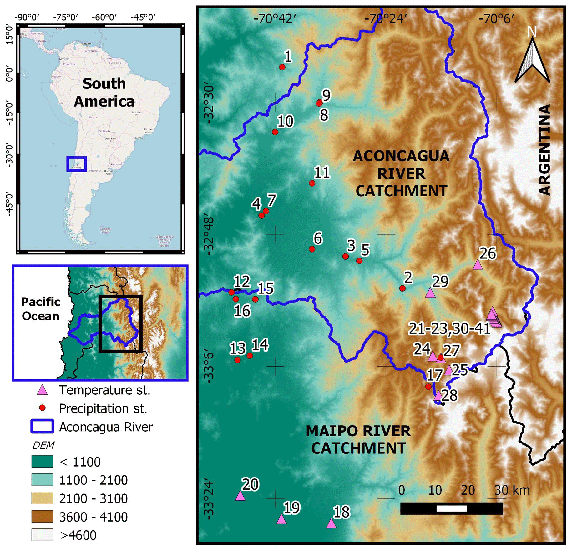
Figure 1 Temperature and precipitation gauges in the catchment with available data during the period of analysis. Further details of the gauges are provided in Appendix A. Upper left panel contributed by © OpenStreetMap contributors 2019. Distributed under a Creative Commons BY-SA license.

2.1 Climate settings

The climate within the Aconcagua catchment is Mediterranean, close to semi-arid conditions (Ohlanders et al., 2013). Annual average precipitation is approximately 350 mm; however, most of this is concentrated during the austral winter (frontal rainstorms during June, July and August), when the South Pacific anticyclone retreats from the region (Falvey and Garreaud, 2007; Montecinos and Aceituno, 2003). This is complemented by occasional convective storms (Garreaud et al., 2009; Viale and Garreaud, 2014). Furthermore, precipitation is also highly influenced by orographic effects, with the windward slope of the Andes having much more precipitation during winter compared to the leeward side (Viale and Garreaud, 2015; Viale and Nuñez, 2011). There are few wind gauges in the area, which hinders understanding of the small-scale preferential wind directions and their influence on precipitation. However, it has been reported that at a macroscale the prevalent direction is west to east (Castro et al., 2014; Garreaud et al., 2009).

The occurrence of solid or liquid precipitation is determined by the location of the zero isotherm during winter; however, above 3000 m a.s.l., low temperatures prevail and precipitation is mostly snowfall. This thermal regime allows a relevant presence of snowpack and glaciers (e.g. Juncal Norte; Janke et al., 2017; Ohlanders et al., 2013).

There is relevant inter-annual variability in the climate variables related to El Niño and La Niña phases (ENSO – El Niño–Southern Oscillation; Garreaud et al., 2009). La Niña is an anomalous cooling of the southeastern Pacific, leading to dry conditions in central Chile when the Pacific anticyclone strengthens, while wet conditions occur during El Niño (Montecinos and Aceituno, 2003; Pellicciotti et al., 2007). Inter-decadal variability related to the Pacific Decadal Oscillation may also affect the case study, although the causes and impacts of these low-frequency fluctuations are less understood than those of ENSO (Garreaud et al., 2009).

Streamflow peaks at the beginning of the austral summer, although it remains high between late spring and summer (Pellicciotti et al., 2007; i.e. the dry season). This means that during this period almost all runoff comes from snowmelt and glacier melt, although the contribution from the latter seems to be relevant during very dry years only (Ohlanders et al., 2013).

2.2 Precipitation and temperature gauges

Observations of daily average temperature and precipitation in the catchment were sourced from the Chilean General Water Directorate (DGA) and the Chilean Meteorological Directorate (DMC) through the Chilean Centre for Climate and Resilience Research (CR2) databases (http://www.cr2.cl/recursos-y-publicaciones/bases-de-datos/, last access: November 2018). Most of these gauges are located in lowlands, whereas the mountain areas are sparsely monitored, with the only available gauges sourced from mine projects in the area. Amongst these high-elevation gauges operated by mining companies, there are two that record liquid and solid precipitation (sites 27 and 17; see Appendix A for more details). The latter were transformed to snow water equivalents (SWEs) before being analysed here.

These data were complemented with information from the Universidad de Chile (Ohlanders et al., 2013; available for some months only) and with measurements done by ETH Zurich in the 2008–2009 summer season (sites 21–23 and 30–41 in Fig. 1; Ragettli and Pellicciotti, 2012; Pellicciotti et al., 2010). The latter were available during a very short period, but the measurements were done near a major glacier and in a different sub-catchment from the one where the private companies installed their gauges. Thus, they provide valuable information for testing the interpolation approaches.

A total of 42 gauges were used in the project: 18 of them measured precipitation and 24 measured temperature. The 42 gauges covered 41 sites, with one site (site 27) having both temperature and precipitation gauges. The locations of the temperature and precipitation gauges are shown in Fig. 1, while further details of the gauges (including the periods with information available and the percentage of missing values) are provided in Table A1 in Appendix A.

The period of analysis spans from September 2008 to August 2013, as most of the data obtained from the high-elevation gauges were restricted to these years. Although not long enough to analyse long-term trends, the selected period allows testing of the interpolation approaches over both dry and wet years. Figure 2 provides an overview of the data by showing the monthly average temperature at four representative gauges over the 5-year period of analysis. In addition, Fig. 3 shows monthly average precipitation and monthly observations at three representative gauges throughout the same period (see Fig. 1 for the location of these gauges).

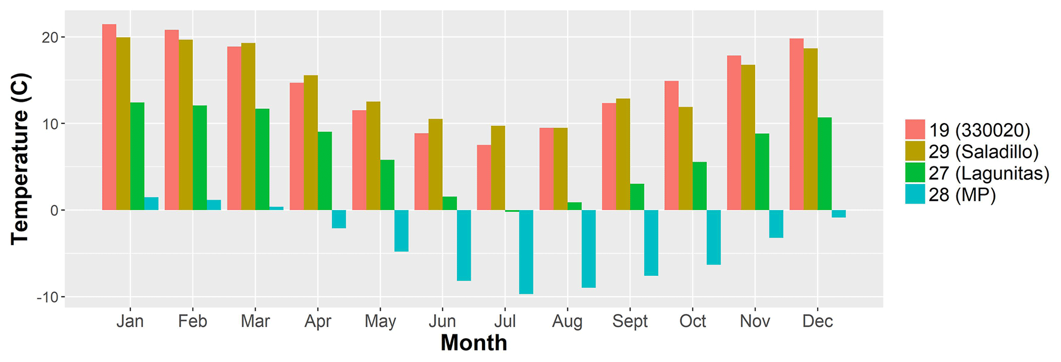
Figure 2 Monthly temperature averaged over the period of analysis, September 2008–August 2013, for four of the gauges in the catchment. The numbers in the legend correspond to those in Fig. 1, while the text in parenthesis is the names of the gauges: 330020 (527 m a.s.l.), Saladillo (1580 m a.s.l.), Lagunitas (2765.5 m a.s.l.) and MP (4250 m a.s.l.).

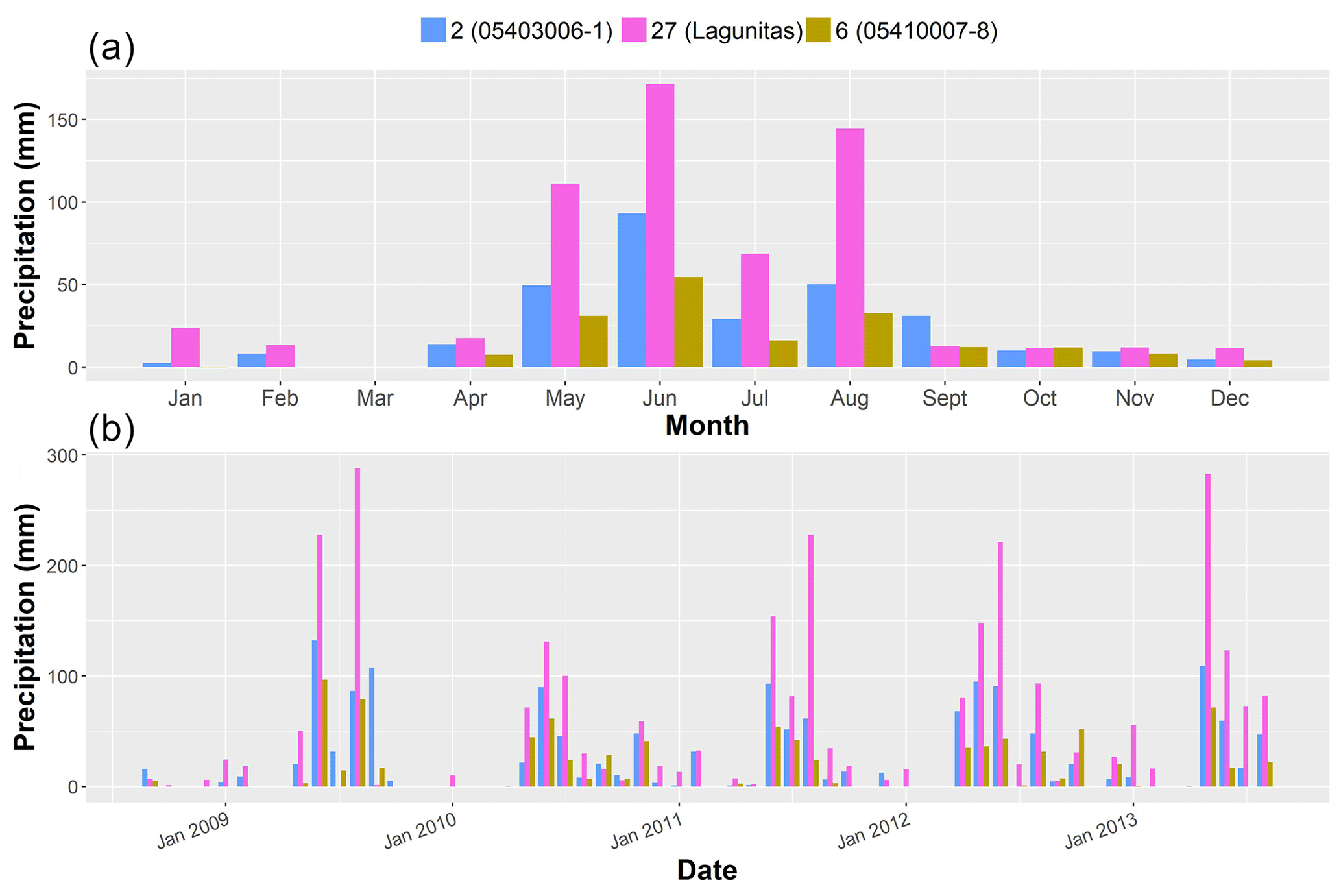
Figure 3 (a) Monthly average precipitation and (b) monthly precipitation over the period of analysis (September 2008–August 2013) for three of the gauges in the catchment. The numbers in the legend correspond to those in Fig. 1, while the text in parenthesis is the names of the gauges: Lagunitas (2765.5 m a.s.l.), 05410007-8 (820 m a.s.l.) and 05403006-1 (1290 m a.s.l.).

Many of the precipitation and temperature data from government institutions have previously been published (Castro et al., 2014; Jacquin and Soto-Sandoval, 2013; Vicuña et al., 2011; Ragettli et al., 2014; Zambrano-Bigiarini et al., 2016), and it has been reported that the precision of the DGA precipitation gauges is 0.1 mm (Castro et al., 2014). In addition, the characteristics of the gauges used by Pellicciotti et al. (2008) were reviewed, and the gauge precision was deemed sufficient for the purposes of this project. In order to complement this, data quality was analysed using double mass plots and plots of the relationship between elevation and the climate variables. This led to the exclusion of precipitation measurements at site 26. Furthermore, all precipitation observations at site 29 were also excluded following the suggestion from one of the mining companies, which stated that the gauge at this site had technical issues when measuring solid precipitation. The temperature measurements at both sites did not show any anomaly. No further issues with data quality were noted.

2.3 Spatially distributed datasets

To complement the point observations, the CHIRPS satellite product (Funk et al., 2015) was used. Although there is a wide range of products available, this selection was done taking into account the good performance of this product in Chile, as reported by Zambrano-Bigiarini et al. (2016) and its spatial resolution (0.05^∘ pixels). Most other products (e.g. TMPA 3B42V7, MSWEP and PGFv3) are relatively coarse for the size of the catchment (0.25^∘ pixels). CHIRPS does not include estimates of temperature and therefore was only used to support interpolation of precipitation.

The WorldClim (WC) Version 1 maps (Hijmans et al., 2005) were a further source of data. WorldClim was suitable due to its spatial resolution (1 km) because it provides both temperature and precipitation values, and as for CHIRPS, because it is available worldwide and so may be used to support interpolation in any case study.

WC data provide a historical average for each one of the 12 calendar months (one map for every month) and originate from a statistical analysis of weather observations worldwide between 1950 and 2000, through an algorithm included in the ANUSPLIN interpolation package (Hutchinson, 2004), using latitude, longitude and elevation as independent variables in a regression. The developers of the WC data warn about its potential inaccuracies in mountainous areas (Hijmans et al., 2005). Therefore, the WC data were used only to complement point observations or as a benchmark for testing other interpolation approaches.

Although different in essence, both WC and CHIRPS can be used as a complement to point observations to construct daily or monthly interpolated fields. None of the selected gauged data were used as inputs in the construction of WC or CHIRPS (the name of the gauges used to calibrate CHIRPS can be checked in UCSB, 2019); furthermore the 5-year period of analysis here does not overlap with the period used to develop WC.

The third spatial dataset used was a digital elevation model (DEM) based on the Shuttle Radar Topography Mission (SRTM; Jarvis et al., 2008), with a spatial resolution of 90 m. The DEM was used to define the elevation in the catchment in order to use this variable in some of the interpolation approaches. Finally, although not spatially distributed, an ENSO index was included to analyse the inter-annual variability in precipitation in the catchment (Wolter and Timlin, 2011).

3 Interpolation of climate data

A stochastic approach, a generalised linear mixed model (GLMM), was compared to simpler deterministic approaches, IDW and LR (Pellicciotti et al., 2014; Ragettli et al., 2014), and two methods based on the residuals between observations and alternative datasets. The first of these two methods uses IDW to interpolate the residuals between WC maps and gauged values (precipitation and temperature), and the second uses IDW to interpolate the residuals between CHIRPS and precipitation observations. These two methods are from now on called WC adjustment (WCA) and CHIRPS adjustment (ChA). A summary of all interpolation approaches including the data required is in Table 1. The following sections describe the methods in more detail and their application.

2012Ragettli et al. (2014)Vicuña et al. (2011)Stehr et al. (2008)Hijmans et al. (2005)Funk et al. (2014)2016Manz et al. (2016)Cameletti et al. (2013)Rue et al. (2009)Rue et al. (2009)2015

Table 1 Summary of approaches to interpolate climate variables.

Before using the covariates mentioned in Table 1 (e.g. WC, elevation, CHIRPS), an analysis of their correlation with the climate variables was done. This included plotting temperature and precipitation observations versus the covariates and computing Pearson correlation coefficients.

3.1 Stochastic approach – GLMM

In addition to including the effects of covariates, GLMMs allow modelling of the spatio-temporal variability in the data (after removing the effect of the covariates) by means of random effects (Faraway, 2016). For example, the temporal correlation of temperature observations in this case study was analysed through an autoregressive (AR1) term (although further alternatives such as random walks could also be used). Furthermore, spatial correlation of precipitation and temperature was modelled as random variables whose covariance matrix is defined by a covariance function (in this case, the Matérn function; Minasny and McBratney, 2005) which depends on the distance between gauges and some spatial parameters (as opposed to intersite dependence functions that do not take into account distance between observations; Yang et al., 2005).

In addition, inference on GLMMs is performed jointly for all the parameters without having to split the estimation problem into separate steps (i.e. one for each time step or doing the covariate regression first and the spatio-temporal analysis second; Hengl et al., 2003). This approach differs from kriging methods, as it avoids using the method of moments to define empirical or experimental variograms (Minasny and McBratney, 2005) and the subsequent adjustment of a theoretical variogram through a curve-fitting exercise (Ecker and Gelfand, 1997; Müller, 1999), as sometimes done for kriging applications in hydrology (Goovaerts, 2000; Nerini et al., 2015). Further details of GLMMs and the different alternatives to model spatio-temporal variables can be found in Faraway (2016), Rue et al. (2009), Lindgren et al. (2011) and Cameletti et al. (2013).

The main drawback of using GLMMs with the Bayesian approach, as done here, is the computational requirements of the classical simulation-based methods such as the Markov chain Monte Carlo (MCMC; Cameletti et al., 2011) method. However, here we use the integrated nested Laplace approximation together with the stochastic partial differential equation approach (INLA–SPDE; Rue et al., 2009; Lindgren et al., 2011; Cameletti et al., 2013), which represents a computationally efficient way to do approximate Bayesian inference on GLMMs (Rue et al., 2009).

In this approach, the climate variables in the case study (temperature and precipitation) are assumed to be realisations (e.g. observations) of a spatio-temporal process (random field) of the following form:

$$\begin{array}{}\text{(1)}& Y(s,t)\equiv \mathit{\left\{}y\right(s,t):(s,t)\in \mathbb{D}\subseteq {\mathbb{R}}^{\mathrm{2}}\times \mathbb{R}\mathit{\}},\end{array}$$

where s and t denote the spatial location and time. This process has a mean μ and covariance function Cov$\left(y\right(s,t),y(s{}^{\prime },t{}^{\prime }\left)\right)={\mathit{\sigma }}^{\mathrm{2}}C\left(\right(s,t),(s{}^{\prime },t{}^{\prime }\left)\right)$ (Blangiardo et al., 2013; Cameletti et al., 2013). Assuming that climate observations, $\mathbf{y}=\mathit{\left\{}y\right(s_i,t),i=\mathrm{1},\mathrm{\dots },N,t=\mathrm{1},\mathrm{\dots },T\mathit{\}}$, follow an exponential family probability distribution function (PDF), μ_i can be connected to a structured additive predictor η_i through a link function g( ) as shown below (Rue et al., 2009):

$$\begin{array}{}\text{(2)}& \begin{array}{rl}& g\left(\mathit{\mu }(s_i,t)\right)=\mathit{\eta }(s_i,t)=\mathit{\alpha }+\sum _{j=\mathrm{1}}^{n_f}{f}^{\left(j\right)}\left(u_{j(s_i,t)}\right)\\ & +\sum _{k=\mathrm{1}}^{n_{\mathit{\beta }}}{\mathit{\beta }}_k{z}_{k(s_i,t)}+\mathit{ϵ}(s_i,t),\end{array}\end{array}$$

where $\mathit{x}=\left(\mathit{\alpha },\mathit{\left\{}{f}^{\left(j\right)}\right(.\left)\mathit{\right\}},\mathit{\left\{}{\mathit{\beta }}_k\mathit{\right\}},\mathit{\left\{}\mathit{\eta }\right(s_i,t\left)\mathit{\right\}}\right)$ is the vector including the Gaussian latent processes (i.e. the parameters describing the random field), $\mathit{ϵ}(s_i,t)\sim N(\mathrm{0},{\mathit{\sigma }}_{\mathit{ϵ}}^{\mathrm{2}})$ is the random error component, the $f^{\left(j\right)}\left(u_{j(s_i,t)}\right)$ values are functions of covariates u and the β's are the multipliers of covariates z.

For temperature, the model in this project was defined based on that described in Cameletti et al. (2013) and Cameletti et al. (2011) for particulate matter, with daily time steps. This selection was done taking into account that both variables are affected by their values in previous time steps but also that both of them have a spatial correlation. The model is described as follows:

$$\begin{array}{}\text{(3)}& {\displaystyle }& {\displaystyle }y(s_i,t)=z(s_i,t)\mathit{\beta }+\mathit{\xi }(s_i,t)+\mathit{ϵ}(s_i,t),\text{(4)}& {\displaystyle }& {\displaystyle }\mathit{\xi }(s_i,t)=a\mathit{\xi }(s_i,t-\mathrm{1})+\mathit{\omega }(s_i,t),\end{array}$$

where y(s_i, t) represents a realisation of the Gaussian field $Y(.,.)$ for site s_i and time t, $z(s_i,t)=\left(z_{\mathrm{1}}(s_i,t),\mathrm{\dots },z_p(s_i,t)\right)$ values are the covariates (fixed effects), β's are the coefficients of the covariates, ϵ is the measurement or observation error component, both serially and spatially uncorrelated ($\mathit{ϵ}(s_i,t)\sim N\left(\mathrm{0},{\mathit{\sigma }}_{\mathit{ϵ}}^{\mathrm{2}}\right)$), and ξ is defined as a 1st-order autoregressive (AR1) component with spatially correlated innovations ω(s_i,t) (a is the parameter of the AR1 process). The covariates included latitude, longitude, elevation and WC. Data from WC maps were included in the model as covariates after extracting the values of the pixels containing the gauges.

The spatio-temporal model for precipitation was defined based on previous experiences of applications of INLA–SPDE for this variable. This involved dividing the analysis into occurrence (Eq. 5) and magnitude (Eq. 6) components, based on Eqs. (8.5) and (8.6) in Blangiardo and Cameletti (2015). However, it was decided to use monthly time steps, as preliminary results of daily runs were far from satisfactory. In addition, CHIRPS and the ENSO index were included as covariates to complement the ones used for temperature:

$$\begin{array}{}\text{(5)}& {\displaystyle }& {\displaystyle }O(s_i,t)\sim \text{Binomial}\left(\mathit{\pi }\right(s_i,t),\mathrm{1}),\text{(6)}& {\displaystyle }& {\displaystyle }{y}^P(s_i,t)\sim \text{Gamma}\left(a\right(s_i,t),b(s_i,t\left)\right).\end{array}$$

Dummy variables for each calendar month were included as additional covariates in order to better represent the strong seasonality of precipitation in the case study (Falvey and Garreaud, 2007; Montecinos and Aceituno, 2003). In this way, the random process for this variable Φ(s_i,t) is spatially correlated but independent of other time steps. The model is described as follows:

$$\begin{array}{}\text{(7)}& {\displaystyle }& {\displaystyle }\text{logit}\left(\mathit{\pi }(s_i,t)\right)=z^P(s_i,t){\mathit{\beta }}^P+\mathrm{\Phi }(s_i,t)+{\mathit{ϵ}}^P(s_i,t),\text{(8)}& {\displaystyle }& {\displaystyle }\log \left({\mathit{\mu }}^P(s_i,t)\right)=z^P(s_i,t){\mathit{\beta }}^P+{\mathit{ϵ}}^P(s_i,t)+{\mathit{\beta }}^{P^{\prime }}\mathrm{\Phi }(s_i,t).\end{array}$$

Both Eqs. (7) and (8) share the same covariate coefficients β^P, but the latter has an extra parameter (${\mathit{\beta }}^{P{}^{\prime }}$) connecting the random field in both equations.

It is acknowledged that other models (i.e. with different random effects) could be tested with these climate variables after changing covariates, spatio-temporal components, the prior distributions (currently we use the default in the R-INLA package) and correlation functions (e.g. as done in Cameletti et al., 2011 for particulate matter), and this represents a subject for future research. However, taking into account the scope of the paper, it was desired to work with existing GLMMs in the literature (or close adaptations) that have been analysed with the INLA–SPDE approach.

3.2 Deterministic approaches

It is assumed that the reader is familiar with IDW and LR. Briefly, the former estimates variables at unsampled locations y(s_j,t) as a function of the inverse of the distance d(s_j,s_i) between s_j and all sampled locations s_i following

$$\begin{array}{}\text{(9)}& y(s_j,t)={\displaystyle \frac{{\sum }_{i=\mathrm{1}}^{n}y(s_i,t)\frac{\mathrm{1}}{\mathrm{d}(s_j,s_i)}}{{\sum }_{i=\mathrm{1}}^n\frac{\mathrm{1}}{\mathrm{d}(s_j,s_i)}}},\end{array}$$

where y(s_i,t) values are the values at the n sampled locations. This method does not consider elevation effects. The LR, on the other hand, uses linear or logarithmic regressions to model the relation between temperature or precipitation and elevation. The regressions could be extended to include all the covariates used in the GLMM; however, the objective here was to apply the methods as they are commonly used to define inputs of hydrological and water resources models in nearby catchments (Ragettli et al., 2014; Vicuña et al., 2011; Meza et al., 2014).

The WCA method attempts to couple the benefits of the spatial variability in the WC maps and those of the temporal resolution of the observations in a simple way. Likewise, ChA attempts to improve the performance of raw CHIRPS by doing a straightforward merging of this product with observations. These approaches are similar to the residual inverse distance weighting (RIDW) in Manz et al. (2016) or the bias adjustment in Dinku et al. (2014) but, in this case, use WC maps and CHIRPS. First, the residual between observations and WC–CHIRPS is computed at each gauge location at a daily resolution for temperature and at a monthly resolution for precipitation. Then, these residuals are interpolated using IDW to each point in the catchment, and this interpolated surface is added back to the original WC–CHIRPS values. This procedure is repeated for every time step.

For precipitation, due to the spatial smoothing that is inherent to all approaches, it is common to have very low values of precipitation where none is observed. Therefore, a threshold of 1 mm per month was set, below which all values were deemed to be 0.

3.3 Comparison of interpolation approaches

In order to assess the performance of the approaches, one gauge was removed from the group used to interpolate the climate variable, and the set of errors for that gauge were recorded as the difference between the interpolation results for that location and the corresponding observations. After repeating this for all gauges, the concatenated errors are used to calculate the validation metrics. This LOOCV procedure was applied separately for temperature and precipitation and for each interpolation approach.

For temperature there was a total of 24 gauges available; thus, the LOOCV analysed 24 combinations of 23 gauges. For precipitation there were 18 gauges available; thus the LOOCV involved analysing 18 combinations of 17 gauges.

For all tests, the average RMSE was used to assess the performance of temperature and precipitation predictions, following similar comparisons (Cameletti et al., 2013; Manz et al., 2016; Nerini et al., 2015). Being a stochastic approach, for the GLMM this involved the analysis of the expected values of each variable (y in Eq. 3 and y^P in Eq. 6).

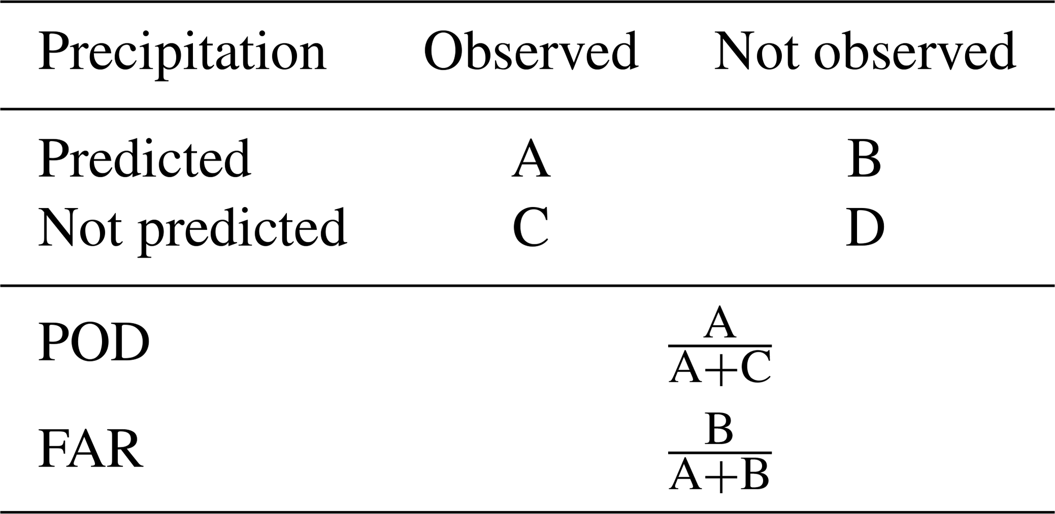
This was complemented with an analysis of the distribution of the residuals. Furthermore, two categorical statistics, the false-alarm ratio (FAR) and the probability of detection (POD; e.g. as applied in Zambrano-Bigiarini et al., 2016), were used to assess the extent to which the model is able to predict precipitation occurrence (see Table 2). These categorical statistics are relevant, even at a monthly timescale, considering that in the case study there are several months without any precipitation; thus accurately simulating its occurrence is not a trivial exercise.

Table 2 Categorical statistics used to assess the capacity of the interpolation approaches to predict the occurrence of precipitation.

3.4 Sensitivity to the number of estimation gauges

The sensitivity of the performance of the different approaches to the number of estimation gauges was also tested. For temperature, only nine gauges with relatively long observation periods were used as estimation gauges in this sensitivity analysis. The other 15 gauges were operational for only one summer period, 2008–2009, and the variability in record length they introduced made it difficult to isolate sensitivity to the number of estimation gauges. These 15, however, remained as validation gauges.

This allowed nine combinations of eight estimation gauges. The nine validation results were averaged for the purpose of the sensitivity analysis. This was repeated using different numbers of estimation gauges: all possible combinations of five and two gauges out of the nine. The sensitivity analysis for the precipitation results was done in a similar way, but this time with all combinations of 14 and 4 gauges.

The sensitivity test was complemented with the estimation of precipitation and temperature values at all locations using raw WC maps and CHIRPS in order to understand the accuracy of these datasets when used independently of the observations. This involved comparing the observed values at each time step with those reported by CHIRPS or the WC maps, which in the latter case meant estimating the climate variables based on the long-term averages in the WC maps.

Regarding the computational requirements, the approximate Bayesian inference approach (INLA–SPDE), which was run on the R-INLA package for R (Rue et al., 2013), required using the Euramoo and FlashLite high-performance computer (HPC) system from the Queensland Cyber Infrastructure Foundation (QCIF). All other interpolation approaches were run on a computer with 16 GB of memory, an i7 processor and four cores.

4 Results

4.1 Preliminary analysis of correlations between covariates and climate variables

Figure 4 shows that monthly temperature values are inversely correlated to elevation (Pearson correlation coefficient $\mathit{\rho }=-\mathrm{0.81}$). The figure also shows a strong correlation between WC values and monthly temperatures (ρ=0.98). Likewise, daily temperature values show considerable correlation with elevation ($\mathit{\rho }=-\mathrm{0.77}$) and WC (ρ=0.93). In contrast, ENSO has a low correlation with temperature (ρ=0.04); thus it was decided not to include this covariate in the GLMM.

Figure 4c and d show that the correlation between CHIRPS and daily precipitation observations is weak but considerably improves when both are aggregated to monthly values (ρ=0.81). The ρ for monthly precipitation and WC values is lower but significant (ρ=0.62), while monthly correlation with elevation is above 0.6 for most months. ENSO shows a weak correlation with precipitation ρ=0.12 (not shown in Fig. 4 for brevity purposes), and similar results are obtained with a time-delayed (1–4 months) ENSO index (i.e. as done in Francou et al., 2004). However, a monthly analysis shows that for several months the correlation is close to ρ=0.5; therefore, it was decided to keep ENSO as a covariate for the precipitation GLMM. These correlations may be stronger in longer-term analyses that cover several Niño–Niña cycles, which last approximately 2–5 years each (Wolter and Timlin, 2011; Garreaud et al., 2017; Montecinos and Aceituno, 2003).

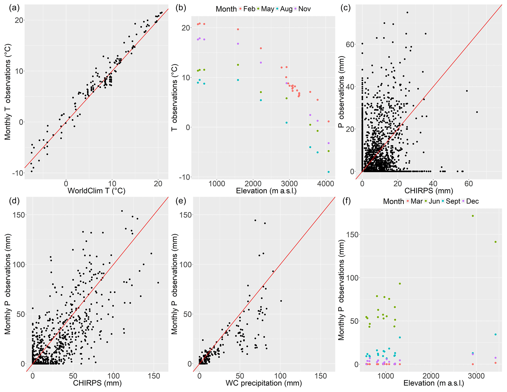
Figure 4 (a) WC values versus monthly aggregated (averaged) temperature values. (b) Elevation of gauges versus average temperature in 4 months. (c) CHIRPS versus precipitation. Daily values for all stations used. (d) Monthly aggregated (sum) CHIRPS versus monthly aggregated (sum) precipitation values. (e) WC values versus monthly aggregated (sum) precipitation values. (f) Elevation of gauges versus average precipitation for 4 months. The red lines correspond to the 1:1 line.

4.2 Temperature results

Table 3 shows the results of all interpolation approaches in terms of the average RMSE of the validation gauges in the LOOCV. It was found that the GLMM and WCA have the best performance, while LR and particularly IDW have larger RMSE values.

Table 3 Temperature RMSEs in the leave-one-out cross validation for each interpolation approach.

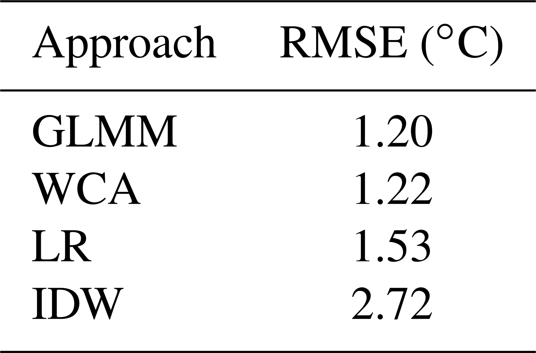
Table 4 shows the results of the sensitivity analysis. As expected, it can be seen that errors increase when the number of estimation gauges decreases. However, values for WCA increase the least, and its loss of performance is relatively small even when only two estimation gauges are used. On the other hand, the performances of all other approaches, including the GLMM, show a sharp decline to the point that some of their RMSE values are comparable with the range of observed temperatures (see Fig. 2).

Table 4 Sensitivity test of the temperature interpolation approaches.

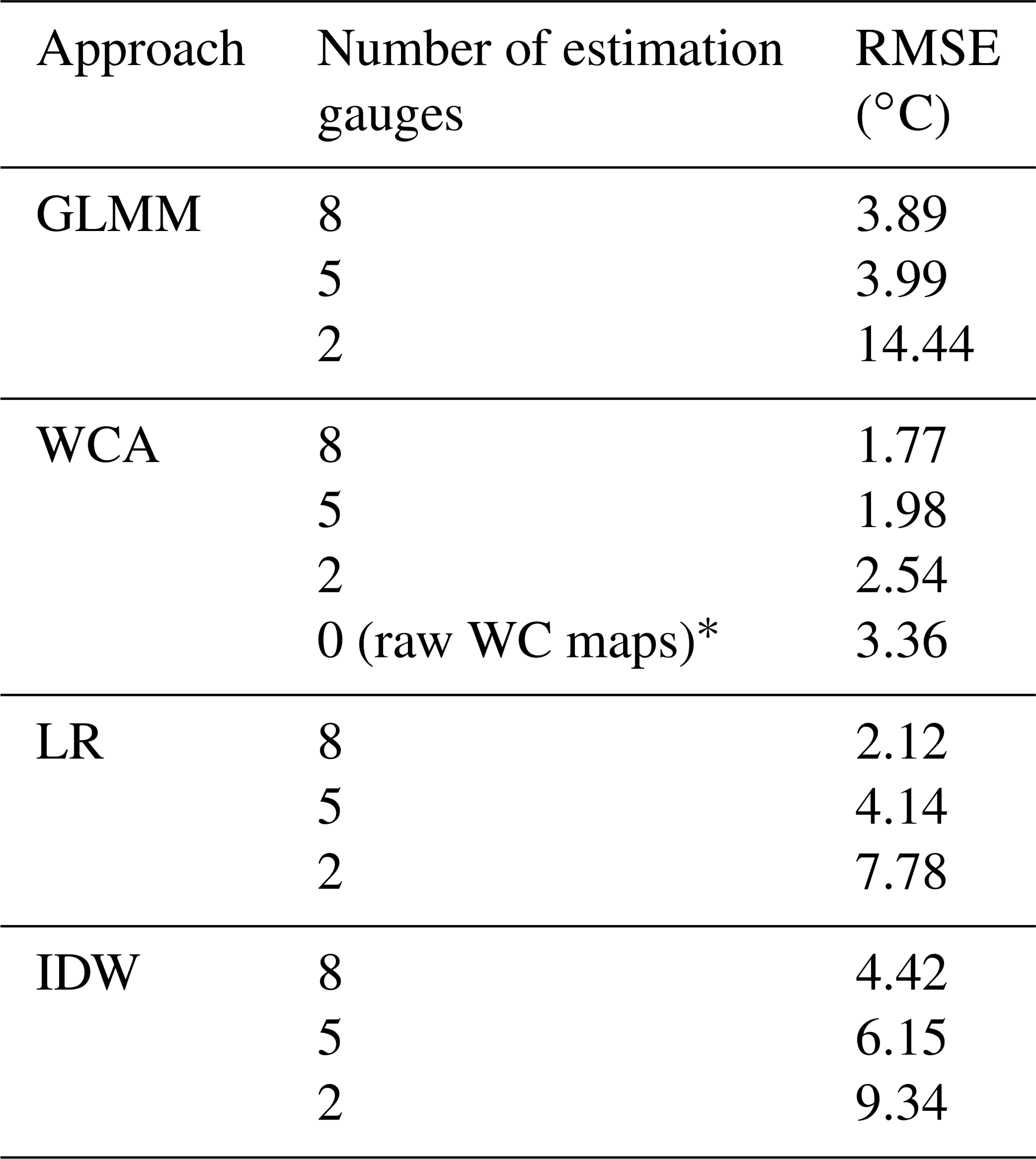
^*Using the monthly long-term values provided by WC to approximate daily temperature at all sites (i.e. one value applied to all days in the month).

Figure 5 illustrates the daily temperature averaged over the 5-year period of analysis for sites 18, 27 and 28 (similar results were found for the rest of the gauges). Values were averaged in this way purely to facilitate visualisation of results, as the daily variability over the 5 years makes it difficult to see which approaches over- and underestimate observations, approximately how much they are over- and underestimated by, and how this changes as a function of the period of the year. The performance metrics were calculated with the non-aggregated data.

In Fig. 5, it can be seen that the GLMM and WCA reproduce the observed temperatures relatively well except for site 28 (the one at the highest elevation – 4250 m a.s.l.). The LR and particularly IDW tend to underestimate temperature at all gauges, except at site 28, where they overestimate it.

In Fig. 5a, the anomalous overestimation of temperature with the LR method around March occurs because during March 2009 all other high-elevation gauges stopped measuring; thus the predictions for site 27 were done with the lower elevation data only. This generated large errors for this gauge and this approach, which may highlight the limitations of the latter when few estimation gauges are available or when it is required to extrapolate results far beyond the elevation of available gauges. This will be further discussed later in this section.

Figure 5 Daily temperature averaged over the 5 years of analysis for gauge (a) site 27 (Lagunitas), (b) site 18 (330019) and (c) site 28 (MP; all curves were smoothed using the LOESS method (Jacoby, 2000) with α=0.045 – this is similar to a moving average and is used to facilitate the visualisation of the main trends only).

Figure 6 shows histograms of the validation residuals. It can be seen that the GLMM, WCA and LR give residuals that are more or less evenly distributed around zero, although those of the GLMM are more peaked. The distribution of IDW residuals is strongly multi-modal, indicating consistent over- or underestimation at particular gauges. Figure 7a shows the relationship between temperature RMSE values and elevation.

Figure 6 Residuals of the temperature LOOCV for each interpolation approach.

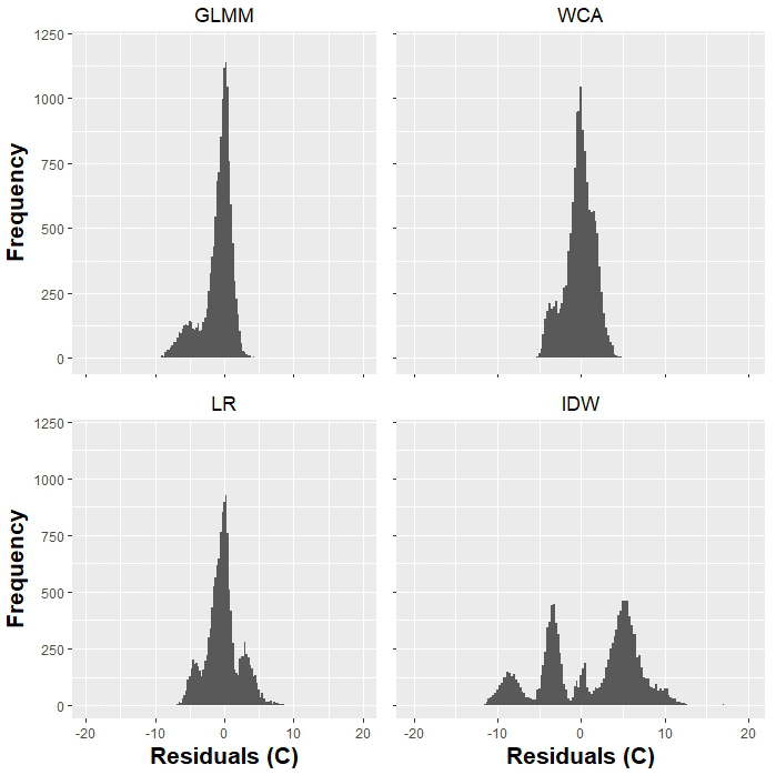
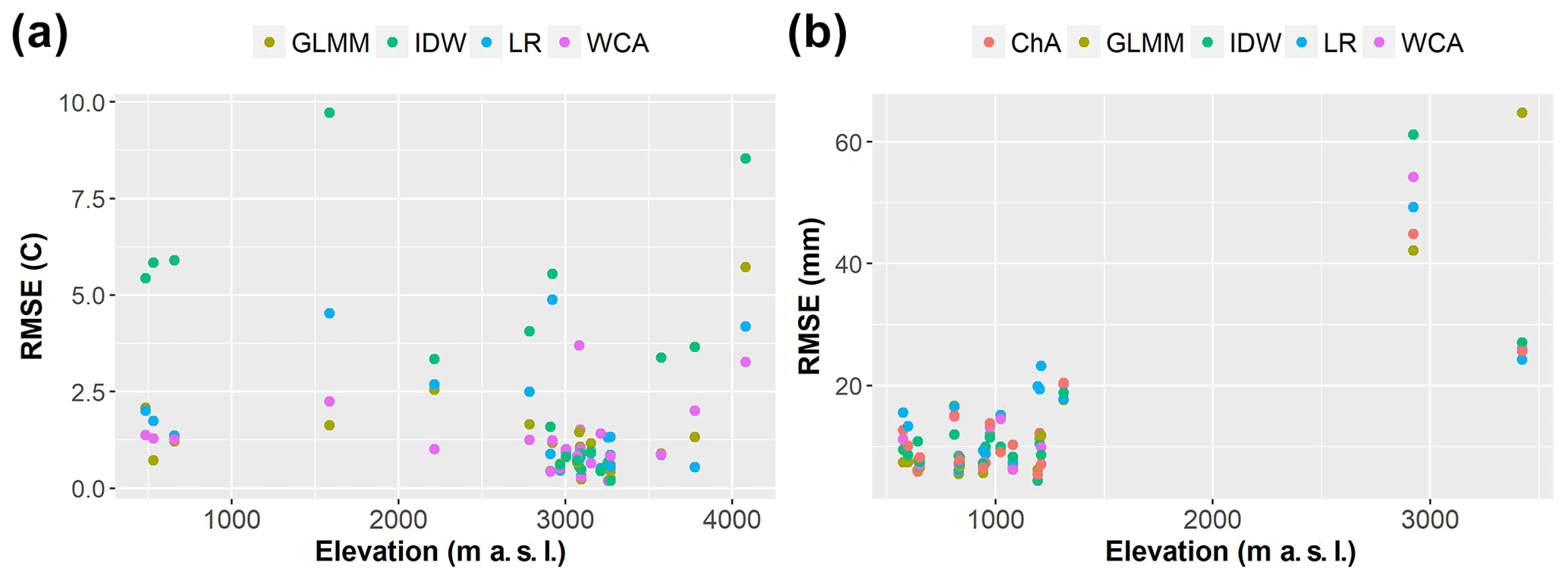
Figure 7 (a) Elevation of gauges vs. average temperature RMSE in the LOOCV. (b) Elevation of gauges vs. average precipitation RMSE in the LOOCV.

4.3 Precipitation results

Table 5 shows that the performances of all interpolation approaches are relatively similar, in terms of RMSE, although ChA has slightly smaller RMSE values. All POD indices are above 90 %, although WCA and IDW have values closer to 100 %. Differences in FARs are larger, as the GLMM has a ratio of only 7.1 %, which is almost half that for LR and ChA and less than a third of that of IDW and WCA.

Table 5 Precipitation results in the leave-one-out cross validation for each interpolation approach.

Table 6 shows the sensitivity of performances to reductions in the number of estimation gauges. It can be seen that the GLMM is quite sensitive to these changes, and its RMSE performance decreases sharply when moving from 17 to 14 gauges and even more from 14 to 4 gauges. Its POD and FAR remain similar. The RMSE performance of the other four approaches decreases by a similar rate (3–4 mm) when moving to 14 gauges, although LR and ChA have a lower POD and FAR. When moving from 14 to 4 gauges ChA shows the smallest increase in RMSE, followed by WCA, while LR has a large increment. PODs and FARs of these four methods remain similar when moving to four gauges, except for the LR POD, which drops by around 6 %.

Table 6 Sensitivity test of the precipitation interpolation approaches.

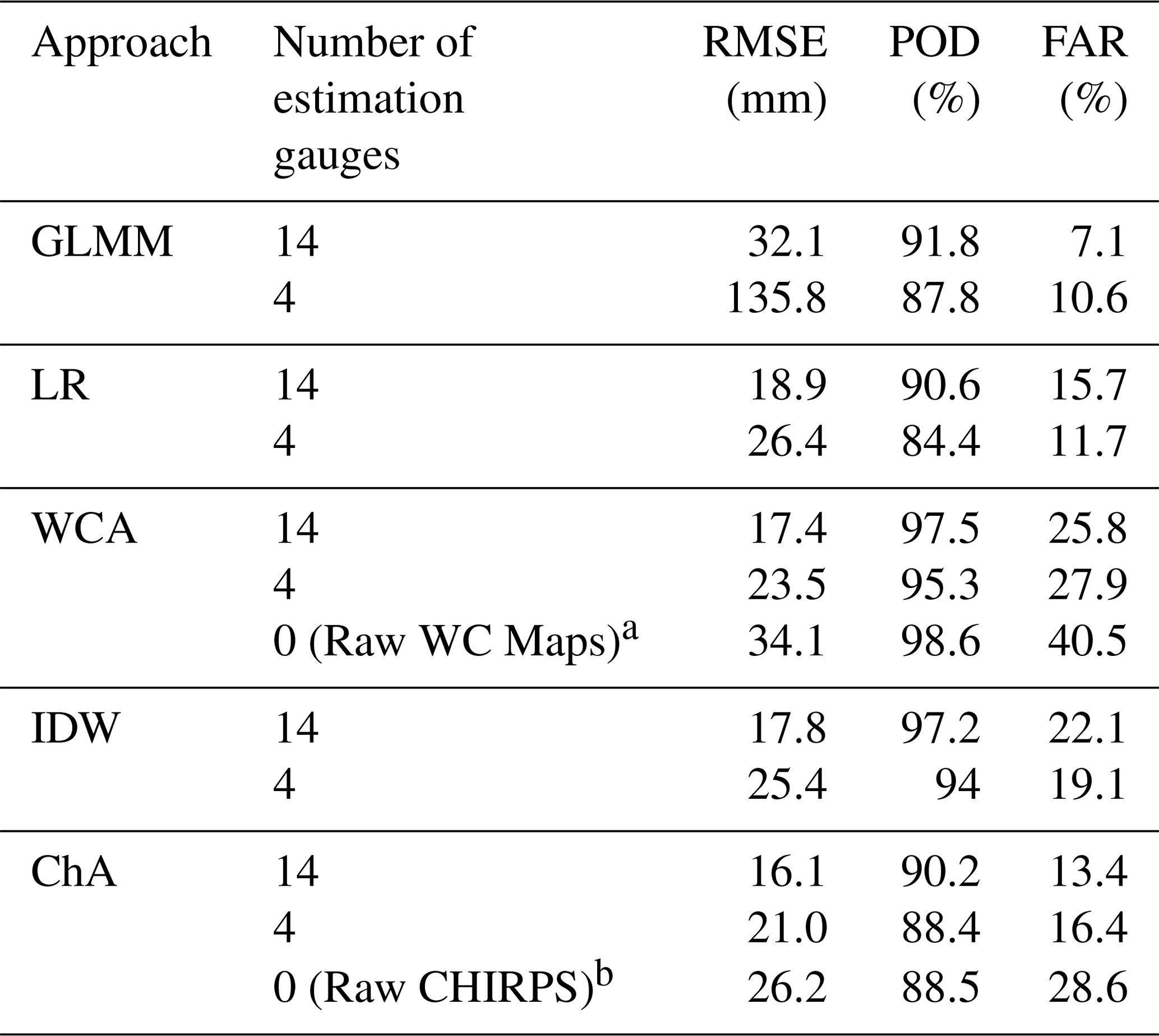
^a Using the monthly long-term values provided by WC to approximate monthly precipitation at all sites.
^b Using the monthly CHIRPS values at all sites.

When these values are compared with raw CHIRPS and WC values, it can be seen that the performance of both alternative datasets by themselves is not competitive when there are 17 or 14 gauges available. The accuracy of CHIRPS gets closer to that of the interpolation approaches when only four gauges are used, suggesting its potential value for especially poorly gauged regions; however, still, ChA and WCA perform better with four estimation gauges.

Figure 8 shows the observed and simulated monthly precipitation values for three representative gauges. Figure 8a shows the performance of the low-elevation gauge at site 1, which is representative of the performance at the other low-elevation gauges. It can be seen that most approaches reproduced observed precipitation at this lowland gauge well compared to the high-elevation gauges. It can also be seen that IDW and WCA predicted small amounts of precipitation in several months during the dry season when no precipitation was observed, which causes a larger FAR for both of them (see Table 5).

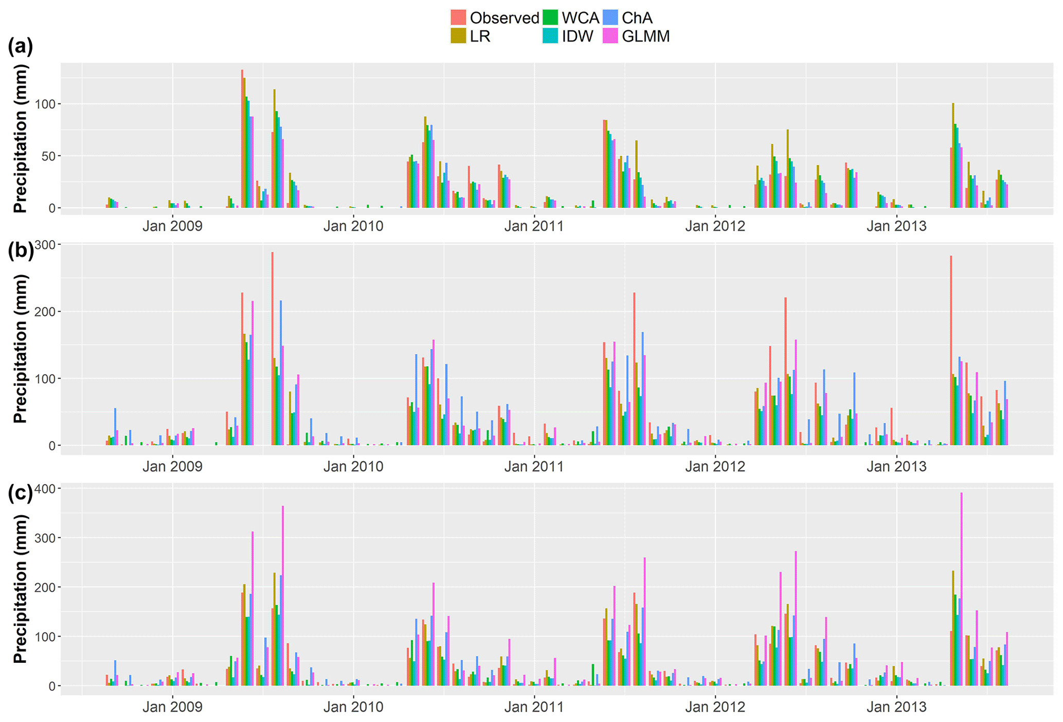
Figure 8 Validation monthly precipitation estimates for sites (a) 1 (05200007-6), (b) 27 (Lagunitas) and (c) 17 (Los Bronces).

Figure 8b shows the performance of all approaches for site 27, which is in the mountains, at 2765 m a.s.l. In this plot it can be seen that observed precipitation is larger than in the lowlands and that all approaches fail to reproduce observations with the level of accuracy seen for the lowland gauge (see Fig. 8a). Figure 8c illustrates results for site 17, the highest of the precipitation gauges (3420 m a.s.l.). Once more, larger errors can be seen compared to the gauges in the lowlands, particularly for the GLMM, although this approach has the best results in site 27.

This behaviour can be better appreciated after plotting the elevation of the gauges versus their average RMSEs (see Fig. 7b). While RMSE values below 1500 m a.s.l. are rarely above 20 mm, all the RMSE values of the two gauges above 1500 m a.s.l. are above this threshold, some of them are beyond 40 mm and two are above 60 mm. This suggests that the performance of all approaches is likely to be determined by inaccuracies at high-elevation gauges, where frontal systems interact with the topography to create high precipitation during the wet season.

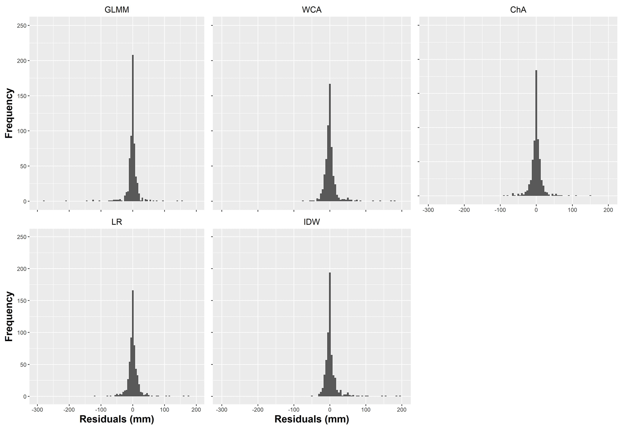
Regarding the distribution of residuals (see Fig. 9), all approaches show values that are more or less equally distributed around zero. The GLMM residuals are particularly peaked at zero; nevertheless, its greater number of very large residuals gives the GLMM a higher RMSE than ChA, WCA or IDW.

Figure 9 Residuals of the precipitation LOOCV for each interpolation approach.

5 Discussion

The LOOCV analysis of air temperature in Sect. 4.2 shows that for this case study, the GLMM and the WCA have the best performance (i.e. smallest RMSE values – see Table 3). These results, and those of LR, are comparable with those obtained from similar analyses in the USA and Canada (Stahl et al., 2006; Wu and Li, 2013). However, compared to the GLMM, WCA has fewer computational requirements and is thus easier to implement (i.e. WCA was run on a desktop computer, as described in Sect. 3.4, while the GLMM was run on 20 HPC cores in parallel).

On the other hand, IDW has the largest temperature errors, and this, together with the skewed and multi-modal nature of its residuals, shows the limitations of this approach. Figure 5c and Fig. 7a suggest that IDW residuals can sometimes be related to the high elevation (e.g. site 28) or isolation (e.g. site 29) of gauges. Temperature observations from the 2008–2009 summer season have the best RMSE values for IDW, but this is likely to be due to the proximity and quantity of gauges in this period.

In terms of the influence of the elevation of gauges on temperature results, WCA, LR and the GLMM show similar performance across all elevations, although the GLMM has an outstanding error at the highest gauge (site 28). This may suggest that compared to WCA and LR, this approach is more sensitive to the extrapolation of results beyond the altitude ranges of the estimation gauges.

Furthermore, it was found that the quality of results of the GLMM is particularly sensitive to the number and location of gauges measuring temperature. As shown in Table 4, the RMSE for this approach rises sharply when only eight (3.89 ^∘C), five (3.99 ^∘C) and two (14.44 ^∘C) gauges are used to estimate its parameters. The performances of IDW and LR also decrease considerably (RMSE of 9.34 and 7.78 ^∘C respectively, with only two gauges) to the extent that using the raw WC maps for this case study (RMSE of 3.36 ^∘C) may be preferable to any method other than WCA once the density of gauges becomes low.

On the other hand, WCA is quite resilient to the reduction of estimation gauges. Even with two estimation gauges the average RMSE was only 2.54 ^∘C. This may be because the raw WC maps have internalised the average effect of elevation, longitude and latitude through the long-term analysis (a worldwide generalisation), which can then be adapted to local conditions by including a small number of gauges. This suggests that WCA is an accurate and easy-to-use alternative for modelling air temperature in the case study.

Regarding precipitation, the LOOCV shows that all approaches have similar performances in terms of RMSE, although the simple merge of CHIRPS and observations (ChA) has a slightly better value (12.8 mm). However, the GLMM also stands out due to its lower FAR (7.1 %), which may be a positive outcome of separating the analysis of precipitation into occurrence and magnitude. This could also be related to the fact that the GLMM analyses the randomness of occurrences and their spatial correlation (see Eq. 7), thus limiting the possibility of one or few gauges with non-zero precipitation overly influencing the precipitation estimate at all points (i.e. smoothing).

As opposed to this, other alternatives, particularly WCA and IDW, tend to predict precipitation when at least one (IDW) or even when no gauges (WCA – due to the inclusion of long-term averages) record non-zero values. This is evident from the prediction of dry-season precipitation events that were never observed (see Fig. 8). Preliminary results obtained using a different threshold (0.3 mm) for the detection of precipitation were similar; thus, the preference for GLMM in terms of FAR and POD performance seems not to be sensitive to the selection of this threshold.

When the precipitation interpolation approaches are tested with a reduced number of estimation gauges, it is found that the RMSE values of the GLMM rise drastically (beyond 100 mm with four gauges only). Once more, this suggests that compared to the alternatives, in this case study the GLMM is more sensitive to the number and distribution of estimation gauges. The importance of the latter is highlighted when using only 14 gauges for model estimation but including at least one of the high-elevation gauges at site 17 (Los Bronces) or site 27 (Lagunitas). This gives an RMSE of 19 mm, which is considerably less than the average RMSE for the GLMM with 14 gauges (32.1 mm).

The other precipitation interpolation approaches decrease their performance at a similar rate to each other when facing a reduction in the number of estimation gauges. As shown for the LOOCV (see Fig. 7B), this may be because errors at high-elevation gauges strongly influence the overall RMSE. When only four gauges are included, however, ChA and to a lesser extent WCA show better RMSE values (21 and 23.5 mm respectively), although the former has a relatively low POD (88.4 %) and the latter a larger FAR (27.9 %). It was also found that CHIRPS as a stand-alone product is a useful alternative to the interpolation approaches when four or fewer gauges are available, with only a marginally worse RMSE value than IDW and a better RMSE than LR and GLMM (RMSE =26.2 mm, POD m=88.5 % and FAR =28.6 %).

The results in this paper show how simple approaches, which can be easily reproduced elsewhere, may perform at least as well as other more complex or more commonly used approaches in a catchment with sparse monitoring networks and complex climate dynamics. Based on this evidence and its simplicity, it would be desirable to use WCA to estimate temperature in this case study. For precipitation, ChA or WCA may be preferable, unless the modeller is particularly interested in the occurrence of precipitation in the dry season, in which case the GLMM would be desirable if computational requirements are not an issue and there is a reasonable coverage of gauges. Analyses of further case studies are required to test the generality of these findings.

Beyond the issues with the number and location of gauges to estimate the parameters of the GLMM, this paper shows how approximate Bayesian inference methods can be applied to estimate parameters of these models in a hydrological context. Despite there being high computational requirements with the R-INLA package, these are lower than those of MCMC, and this facilitates the use of GLMMs. It would now be useful to test if the benefits of GLMMs and Bayesian approaches discussed in this paper and in the non-hydrology literature (Pilz and Spöck, 2008; Ecker and Gelfand, 1997) can equally be achieved by stochastic approaches like kriging and generalised linear models (GLMs) that are more common in hydro-climate applications. It would be particularly interesting to analyse how these approaches behave in well and poorly monitored regions and how this influences hydrological modelling.

Results in this case study are of course limited by the fact that 15 temperature gauges in the mountain areas were measured during one summer season only. For precipitation, it would also have been desirable to have good-quality gauges between 1300 and 2700 m a.s.l. to better understand what happens between the low- and high-elevation gauges.

6 Conclusions

Interpolation of climate variables is a major field of research in hydrology due to their importance in water resources modelling. This paper compared five approaches to interpolating temperature and precipitation gauged data in a catchment with complex and steep terrain and tested their sensitivity to the reduction of the number of estimation gauges. High-elevation gauges, not previously used before for this type of research, were employed to partially test the ability of the approaches to extrapolate to the high Andes.

For temperature, a generalised linear mixed model (GLMM) reproduced observations in this case study in the best way (i.e. smallest root-mean-squared error – RMSE, in a leave-one-out cross validation – LOOCV), although it was closely followed by a simpler alternative based on merging observations and WorldClim maps (WCA). The latter performed relatively well at all high-elevation points. Inverse distance weighting (IDW) and lapse rates (LRs – i.e. a linear regression using only elevation as a covariate) showed a worse performance.

Furthermore, for temperature, only WCA demonstrated resilience to the reduction of the number of estimation gauges, showing good prospects for supporting hydrological modelling in sparsely monitored catchments. The GLMM, IDW and LR had larger errors to the point that for this case study, for temperature interpolation using few gauges, long-term estimates from WorldClim maps gave better RMSE results.

For precipitation, no alternative was clearly superior in the LOOCV, and this may be because errors in high-elevation points, which were large irrespective of the approach, dominated the RMSE values. ChA showed smaller RMSE values in the sensitivity test (although it had lower probabilities of detection – PODs), which highlights the desirability of the method in this case study unless detecting most months with precipitation was fundamental for the user. The other approaches showed a relatively similar resilience to the reduction of estimation gauges, except for the GLMM, which had a poorer performance, with an RMSE value larger than 100 mm when only four gauges were used.

In terms of the added value of alternative datasets, it was found that in this case study the inclusion of CHIRPS and WorldClim was valuable. Firstly, using the residuals between WorldClim maps or CHIRPS and climate observations represented a simple but efficient method that showed good performance and high resilience when working with few gauges. On the other hand, CHIRPS, as a stand-alone product, was demonstrated to be a useful source of precipitation data when no or few gauges were available.

Appendix A: Gauges used

Table A1 Details of gauges used.

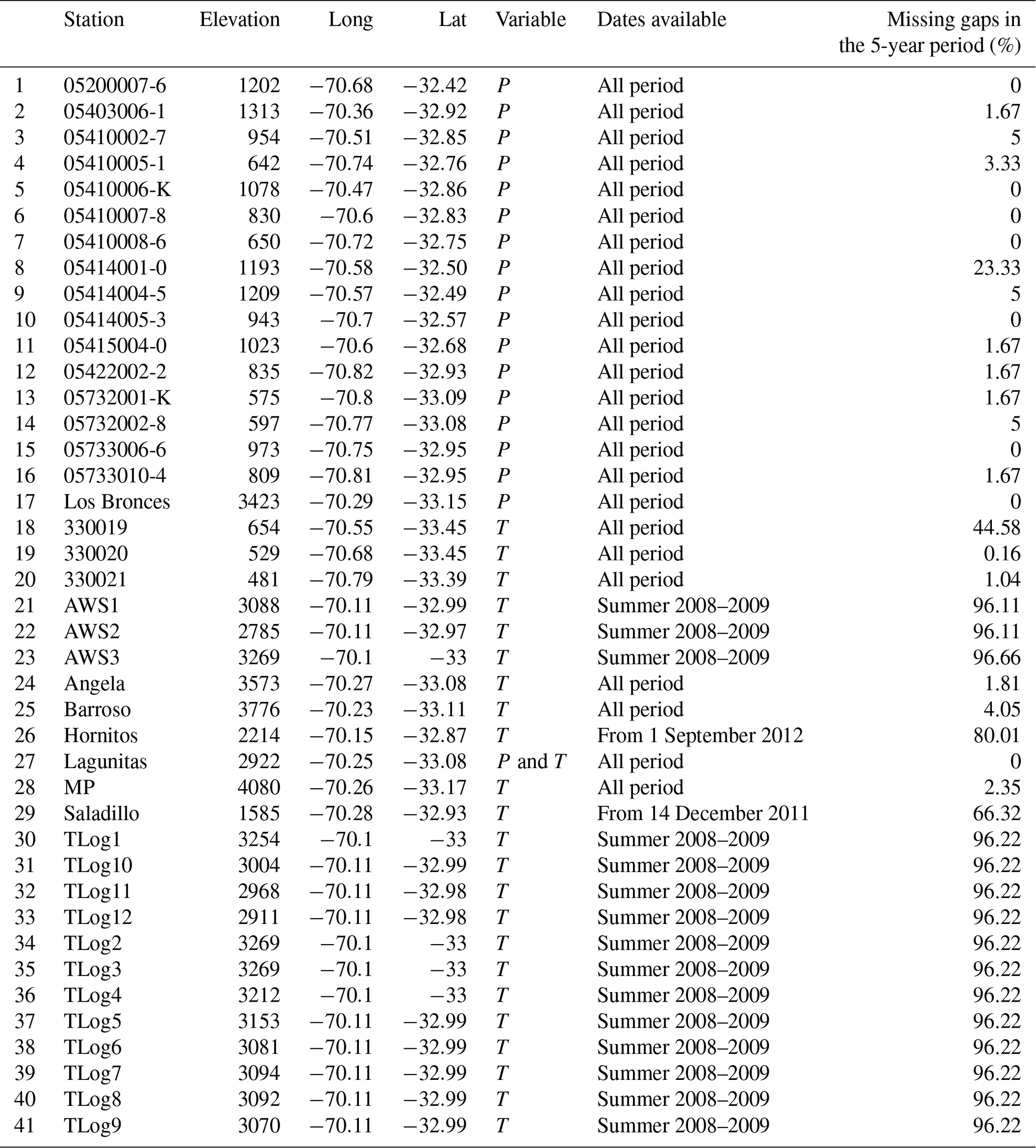
Summer 2008–2009 represents the summer season in the Southern Hemisphere.