Assessing the impacts of hydrologic and land use alterations on water temperature in the Farmington River basin in Connecticut

Aquatic ecosystems can be significantly altered by the construction of dams and modification of riparian buffers, and the effects are often reflected in spatial and temporal changes to water temperature. To investigate the implications for water temperature of spatially and temporally varying riparian buffers and dam-induced hydrologic alterations, we have implemented a modeling system (DHSVM-RBM) within the framework of the state-space paradigm that couples a spatially distributed land surface hydrologic model, DHSVM, with the distributed stream temperature model, RBM. The basic modeling system has been applied previously to several similar-sized watersheds. However, we have made enhancements to DHSVM-RBM that simulate spatial heterogeneity and temporal variation (i.e., seasonal changes in canopy cover) in riparian vegetation, and we included additional features in DHSVM-RBM that provide the capability for simulating the impacts of reservoirs that may develop thermal stratification. We have tested the modeling system in the Farmington River basin in the Connecticut River system, which includes varying types of watershed development (e.g., deforestation and reservoirs) that can alter the streams' hydrologic regime and thermal energy budget. We evaluated streamflow and stream temperature simulations against all available observations distributed along the Farmington River basin. Results based on metrics recommended for model evaluation compare well to those obtained in similar studies. We demonstrate the way in which the model system can provide decision support for watershed planning by simulating a limited number of scenarios associated with hydrologic and land use alterations.

1 Introduction

Aquatic ecosystems can be significantly altered by the construction of dams and modification of riparian buffers, which consist of the trees and shrubs bordering streams and rivers. While the construction and operation of dams and their associated impoundments provide many services, including the generation of electricity, flood control, navigation, water supply, irrigation and recreation (Bednarek, 2001), they can also have a significant impact on ecosystem functions (Brooker, 1981; Ligon et al., 1995; Power et al., 1996). Their effects are often reflected in the spatial and temporal changes to stream temperatures, which play a major role in the function of aquatic ecosystems (Poole and Berman, 2001). For example, studies have shown that releases of warm water from the surface layers of an impoundment can have an impact on cold water fishes, macroinvertebrates and aquatic habitat downstream of the dam (Lessard and Hayes, 2003). Impoundments with long residence times (the ratio of reservoir volume to annual average reservoir outflow) can become thermally stratified, with warm water at the surface (epilimnion) and cold water at depth (hypolimnion) (Niemeyer et al., 2018; Preece and Jones, 2002). In some cases, the cold water is released from the hypolimnion to support or enhance cold water fisheries (Pike et al., 2013; Yearsley, 2009). However, releases of hypolimnetic water can also have deleterious effects on important warm water assemblages of native fishes and other aquatic organisms downstream of the dam (Olden and Naiman, 2010).

Alteration or removal of riparian buffers can also have a significant impact on the physical, chemical and biological characteristics of aquatic ecosystems (Albertson et al., 2018; Sweeney and Newbold, 2014). An assessment of national streams and rivers in 2008–2009 by the U.S. Environmental Protection Agency (USEPA) concluded that a lack of adequate riparian vegetation was the most common stressor in the streams and rivers of the United States that were in poor condition (USEPA, 2013). Shading of solar radiation is one of the many important benefits to aquatic ecosystems provided by streamside buffers of riparian vegetation (Cole and Newton, 2013; Sweeney and Newbold, 2014). Brown and Krygier (1970) found that increases in stream temperature were due to a loss of riparian buffers resulting from the logging practice of clear-cutting in the Pacific Northwest. Studies such as this have played an important part in the creation of legislation that protects aquatic ecosystems, such as the Oregon Forest Practices Act of 1971 (Bladon et al., 2016). In addition to forest harvest, other land uses, including road building, livestock grazing, and mining (McGurk, 1989; Chen et al., 1998), have resulted in the loss of riparian buffers. In the United States, for example, environmental agencies have addressed these issues in terms of Section 303 (d) of the US Clean Water Act by requiring specific programs for riparian buffer restoration that will meet water quality standards for stream temperature. In addition to providing the scientific basis for watershed planning actions that protect or restore streamside buffers, some studies predict that stream channel restoration has the potential to mitigate some of the impacts of a changing climate (Cuo et al., 2009; Justice et al., 2017).

In this study, we develop methods for simulating certain features of dam operations and riparian vegetation that influence stream temperature in the Farmington River watershed in the Connecticut River system. We do so within the context of state space estimation (Schweppe, 1973), as defined in Eqs. S1 and S2 in the Supplement, for which the matrices of the state space estimators can be parameterized from the conservation laws governing momentum and energy (Boyd and Kasper, 2007; Chapra et al., 2008; Cole and Wells, 2002; Pike et al., 2013; Wu et al., 2012; Yearsley, 2009). The model constructs for stream temperature that are based on these conservation laws are sufficiently general to accommodate a broad spectrum of time and space scales, ones that are based on the thermal energy budget for streams and rivers.

Model development often comes with a price, however, because estimating the parameters can become an exercise in solving a highly underdetermined geophysical data analysis problem. This is a problem that depends on time and space scales and model complexity. In the case of model development for complex aquatic ecosystems at high frequencies and small scales, some have approached these issues by limiting spatial and temporal scales and by designing rigorous and extensive data collection programs (Boyd and Kasper, 2007; Glose et al., 2017). State-space models of water temperature, developed at regional and global scales, have a higher level of aggregation for spatial scales and include only the most important components of the thermal energy budget (Yearsley, 2012, 2009).

Working within the broad framework of the conservation of momentum and thermal energy, here we investigate the way in which an integrated state-space model system of hydrology and water temperature (DHSVM-RBM) can be used to characterize the impacts of landscape alteration at intermediate spatial and temporal scales. In the Supplement, we describe the matrices of the nominal solution (Eqs. S5 and S6) for the linearized state-space water temperature model, RBM (Yearsley, 2012, 2009). Using this approach, our goals are to (1) develop and evaluate the nominal solutions for state-space estimates of streamflow and water temperature in the Farmington River basin in Connecticut using methods derived from physical principles and data gleaned from publicly available repositories, and (2) use our model to provide examples from the Farmington River basin of the way in which the models can be used to evaluate water temperature impacts of changes in riparian vegetation and water storage.

2 Background and site description

The Farmington River basin (Fig. 1) has an area of 1559 km² with two main branches, the West Branch and the East Branch. The West Branch is 129.4 km in length and has its source in Hayden Pond near Otis, Massachusetts, while the East Branch is 75.2 km in length with headwaters in the Barkhamsted Reservoir near New Hartford, Connecticut. Land cover for the Farmington River basin, according to National Land Cover Database 2011 (NLCD 2011), is characterized by 58 % of forest and 24 % of developed land with the remaining 18 % comprised of wetlands (8 %), farmland (7 %), and open water (3 %). A total of 73 % of the soils in the Farmington River basin are sandy loams according to the US Department of Agriculture (USDA) Natural Resources Conservation Service (NRCS) States Soil Geographic Database (STATSGO).

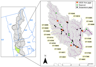
Figure 1 Map of Farmington River basin showing 22 CTDEEP water temperature monitoring sites, 6 USGS flow gage sites and 7 major reservoirs characterized by the two-layer module of DHSVM-RBM.

As was true for the entire Connecticut River basin (Cogbill et al., 2002), deforestation began in the Farmington River basin in the 18th century as European settlers cleared land for agriculture and timber harvesting (Wharton et al., 2004). However, as a result of the decline of the agricultural industry in the State of Connecticut, reforestation began in the later part of the 19th century. More recently, forestlands have decreased again as a result of forest harvest and urban growth. Jeon et al. (2014) reported that the annual rate of loss of forestlands due to permanent changes in land use in Connecticut was 1321 ha yr⁻¹ from 1990 to 2000 and 979 ha yr⁻¹ from 2000 to 2005, particularly in the heavily urbanized counties of Connecticut (Fairfield and New Haven counties). Nevertheless, about 60 % of Connecticut remains in forestland, including the counties of Litchfield and Hartford comprising the Farmington River basin (75 % and 53 % forested, respectively; Wharton et al., 2004).

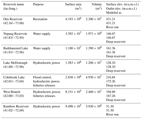
In addition to landscape alterations due to forest transition, the Farmington River basin has experienced considerable development of water management projects for the purposes of water supply, flood control, hydroelectric power generation and recreation. The study of the Farmington River watershed by the Farmington River Watershed Association (2004) reported a total of 409 impounded lakes and reservoirs in the basin. They described most of these as smaller-scale impoundments, many of which were constructed in the early 1900s and are in disrepair or no longer necessary. There are, however, a number of impoundments of sufficient size to have an impact on the aquatic ecosystem of the river basin. For the purposes of this study, we chose to limit our study to seven large reservoirs (Table 1) with the potential for significantly modifying the water temperature regime of the natural system. This includes the five major reservoirs in the Farmington River watershed in Connecticut, Otis Reservoir in Massachusetts and Rainbow Reservoir in the lower Farmington River (Table 1). We modeled Otis Reservoir and Rainbow Reservoir as river-run reservoirs that are vertically well-mixed. As a result, the primary effects of these two reservoirs on stream temperature would be to reduce the amplitude of diurnal variations due to an increase in water depth (Edinger et al., 1968). Nepaug Reservoir, Barkhamsted Reservoir, and McDonough Reservoir are deep reservoirs whose primary function is for domestic water supply. We modeled these reservoirs as comprising two layers, a surface layer (epiliminion) and deep layer (hypolimnion), which stratify vertically. Colebrook Lake and West Branch Reservoir are also treated as deep reservoirs that have multiple functions including flood control, flow augmentation, fishery enhancement, recreation, and generation of hydroelectric power. More details on reservoir representation in the temperature model are provided in Sect. 3.2.

Table 1 Water storage projects in the Farmington River basin modeled with one-dimensional (river run) or two-dimensional (deep reservoir) modules of RBM (m a.m.s.l. indicates meters above mean sea level).

3 DHSVM-RBM model identification

DHSVM-RBM (Sun et al., 2015) integrates the physics-based Distributed Hydrology Soil Vegetation Model (DHSVM; Wigmosta et al., 1994), modified to include a riparian shading module (Sun et al., 2015), into the vector-based version of the semi-Lagrangian stream temperature model RBM (Yearsley, 2009). In addition, we incorporated a module into RBM that simulates certain basic features of deep reservoirs.

3.1 Hydrology and riparian shading model

DHSVM was developed originally to simulate the hydrologic cycle in mountainous terrain (Wigmosta et al., 1994) based on saturation excess mechanisms. Subsequent adaptations have extended the capability of DHSVM to include urban landscapes with impervious surfaces and runoff detention (Cuo et al., 2008), glacier hydrology (Naz et al., 2014), riparian shading (Sun et al., 2015), urban water quality (Sun et al., 2016), and forest–snow interactions in canopy gaps (Sun et al., 2018). As applied in the Farmington River basin, DHSVM simulates the water and energy budget at 3-hourly timescales and 150 m spatial scales for the physical processes of canopy interception, evaporation, transpiration and runoff generation driven by the spatial input of soil, vegetation, topography and climate. The version of DHSVM that we used does not have the capability for simulating the effects of water management projects in the watersheds that regulate streamflows and, as a result, alter the natural hydrograph. Thus, in our study the flows simulated by DHSVM are the unregulated flows. The model limitations and implications are further discussed in Sect. 5.2.

For this study, the riparian vegetation module of DHSVM described in Sun et al. (2015) has been modified to account for spatial and temporal variation in riparian vegetation. The temporal variability of riparian vegetation is described by a monthly-varying extinction coefficient in the Beer's law representation of radiation transmission through the canopy (Wilson and Baldocchi, 2000). This approach is well-suited to the deciduous forests of the northeastern United States, for which the shade density of riparian vegetation varies annually. The capability to include spatial variability provides more information to decision-makers for watershed planning. The spatial variations of riparian vegetation along the longitudinal axes of river segments are characterized by varying riparian vegetation parameters on a stream segment-by-segment basis. Rather than applying basin or subbasin uniform riparian parameters based on `representative' tree species as field data on basin-wide riparian vegetation are often lacking, we estimated the riparian parameters that calculate radiation incident on the stream surface using Google products, literature values and the results from previous studies. We estimated the buffer width and extent of vegetation coverage by sampling all stream segments at about 1000 m intervals using the online tools in Google Maps. We inferred vegetation types (trees and shrubs) from forest surveys (Wharton et al., 2004) and tree height based on tree species identified in Wharton et al. (2004) and studies of the height of hardwoods (Lamson, 1987). In addition, where possible, we compared the height of trees with utility poles using Google Maps Browse Street View, assuming that the average height of wooden utility poles is 15 m. We treated the riparian vegetation parameters estimated in this way as the baseline condition, representative of existing conditions in the watershed.

Table 2 Datasets and sources used for estimating parameters in the model identification process.

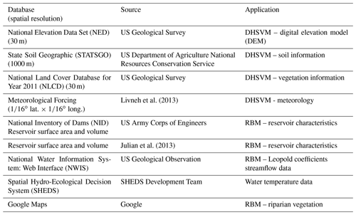
Other DHSVM model input includes gridded meteorological data consisting of precipitation, air temperature, downward shortwave and longwave radiation, wind speed, and relative humidity (Table 2). The 3-hourly meteorological forcing data were disaggregated, using MTCLIM (Bohn et al., 2013; Thornton and Running, 1999), from a daily forcing dataset for the conterminous United States developed by Livneh et al. (2013). We used the DEM from the US Geological Survey (USGS) National Elevation Dataset (NED) rescaled from 1 arcsec (app. 30 m) to 150 m. The soil class map was taken from STATSGO. The land cover data were taken from the USGS NLCD for the year 2011 and rescaled from 30 to 150 m with the Resample tool in ArcGIS.

3.2 Stream and reservoir temperature models

RBM is a one-dimensional, time-dependent model of water temperature for streams and rivers dominated by advection that are well-mixed vertically and laterally. RBM employs a semi-Lagrangian particle-tracking numerical scheme that has proven to be accurate and efficient in riverine systems dominated by advection. The numerical scheme is highly scalable in time and space and has been applied to study the water temperature responses to changing climate, land use and riparian vegetation at watershed and regional scales (Cao et al., 2016; Sun et al., 2015).

For those stream and river segments dominated by advection, we solve the one-dimensional, time-dependent equations for the thermal energy budget (Yearsley, 2012, 2009) (see Supplement). Initial conditions are required for solving difference equations with the form of Eq. (S5) (see Supplement). Errors in estimating initial conditions will introduce uncertainty into the solution only for the time it takes for the particle of water to traverse from its headwaters to its outlet. For example, the West Branch is the longest (129 km) branch of the Farmington River. Assuming a moderate stream speed of 0.5 m s⁻¹, the time of travel associated with an initial parcel in the West Branch would be about three days. Since our simulations span a period of several months, we have assumed the initial water temperature throughout the Farmington River to be 0.0 ^∘C, and that errors associated with initial conditions have been dissipated after a spin-up time that is greater than the travel time of a water parcel from the headwaters to the confluence with the main stem Connecticut River.

Headwater temperatures are the temperatures of the water that enters the surface water at the stream source and can result from rainfall, snow melt or hyporheic flow. They have an important role in the heat budget of stream and rivers, the extent of which depends on the nature of the watershed (Janisch et al., 2012). However, their influence on downstream water temperatures diminishes as a function of stream speed, stream depth and meteorological forcing, reducing the uncertainty associated with errors in estimates as water parcels travel downstream (Yearsley, 2012). Here, as in previous studies (Sun et al., 2015; Wu et al., 2012; Yearsley, 2012, 2009), we used the nonlinear regression of the logistic relationship between air temperature and water temperature from Mohseni et al. (1998). We estimated the parameters, α, β, γ, and μ, in Eq. (S8) (see Supplement) by minimizing the sum of the squared difference between Eq. (S8) and the water temperature at the Connecticut Department of Energy and Environmental Protection (CTDEEP) gage site, referred to as CT15844 (Fig. 1), which is located near the headwaters and has multi-year continuous temperature records located near headwater. We further assumed that the estimates of the parameters for this location could be extended to the other headwaters in the Farmington River basin given that the parameters applied to CT-14442 and CT-14713 gage sites produced reasonable agreement between simulated and observed headwater temperatures (Table 5).

The reservoir module added to the RBM software represents a simplified approach to characterizing those river segments with reservoirs that have long residence times and potential for vertical stratification of water temperature. Based on their volume and outflow rate, we included those reservoirs on significant tributaries that had the potential for developing thermal stratification. Reservoirs included in our study with these characteristics are shown in Table 1. We obtained the reservoir geometry and operating characteristics for those segments in the Farmington River basin with longer residence times (Table 1) from the NID USACE (2015) and Julian et al. (2013). Our approach, similar to that described in Boehlert et al. (2015), Chapra (1997), and Niemeyer et al. (2018), conceptualizes river segments with reservoirs that may stratify as two layers, a surface layer (the epilimnion) and a bottom layer (the hypolimnion). Those stream segments identified as having a reservoir with potential for stratification were treated as multiple cells, depending on reservoir length, for the purposes of estimating the flux of thermal energy across the air–water interface and advective tributary input. For reservoirs with more than one cell, the cells were combined after computing the surface transfer of thermal energy and advective tributary input into a single well-mixed epilimnion and single well-mixed hypolimnion continuously stirred reactors (CSTRs) as in Fig. 2. Specific details of the development of the nominal solutions for both the stream segments dominated by advection and those that may develop an epilimnion and hypolimnion are given in the Supplement.

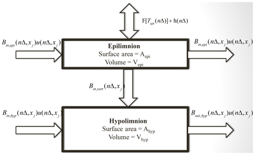
Figure 2 Conceptual model of a continuously stirred reactor (CSTR) for the two-layer reservoir model.

For the purposes of this study only, we assumed that the volumes of the epilimnion and hypolimnion were equal and were constant for the duration of the simulation period and that the outflow from each reservoir was equal to the total inflow. For those reservoirs whose primary function is water supply (Table 1), all outflow was from the epilimnion. In the case of Lake Colebrook, which has a controlled hydraulic sluice and hydropower turbines near the reservoir bottom, we assumed that all outflow was from the hypolimnion. Tributary inflow was placed into either the epilimnion or hypolimnion depending on whether the density of the inflow was lesser or greater than the density of the epilimnion, as in Niemeyer et al. (2018). There are also lakes and impounded segments in the Farmington River with shallow depths and short residence times. We simulated the water temperature in these segments assuming they could be treated as cross-sectionally averaged, well-mixed segments. Furthermore, we assumed that all these reservoirs had constant surface elevation and that the speed of the water parcel U(nΔ,x_j) at time nΔ and location x_j could be estimated from the continuity equation. Stream speeds for those reservoirs in the Farmington River basin described as “River Run” in Table 1 were estimated in this way.

Within the coupling scheme, DHSVM provided DHSVM-RBM hydrologic and meteorological forcing input for each river segment, which was aggregated as the length-weighted average of the gridded 150 m cells that intercept a stream segment as in Sun et al. (2015). RBM makes use of DHSVM stream network file to establish the topology for its numerical solution technique. Stream networks, created in DHSVM with DEMs and ESRI Arcinfo macro language (AML) scripts, are composed of shorter stream segments connected within a network, with unique attributes of length, width, orientation, and Strahler stream order. Stream segment connectivity was used to define the network topology for DHSVM-RBM's particle tracking scheme.

Table 3 Parameters for stream speed and depth in Eqs. (S7) and (S8) (see Supplement) estimated from rating measurements at USGS gages in the Farmington River basin. Coefficients from individual USGS gages are extended to other river segments as shown.

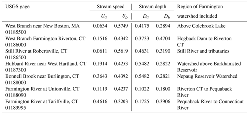
We used inflow and outflow to each segment in the stream network simulated by DHSVM to estimate (1) the depth, D(nΔ,x_j), in one-dimensional, time-dependent formulation of the thermal energy budget (Eq. S14 in the Supplement), and (2) the stream speed, U(nΔ,x_j), in the particle-tracking algorithm (Eq. S6) with the method from Leopold and Maddock (1953). We estimated the parameters, d_a, d_b, u_a and u_b, in Eqs. (S7) and (S8) for the freely flowing segments RBM from the rating curve to stage–discharge relationships at the USGS gage sites shown in Table 3. RBM accommodates spatial variability for the coefficients that describe stream speed and depth as a function of streamflow. However, there are only a limited number of gages from which to estimate their values. We then assumed the parameter estimates at the individual gages could be extended to other stream segments as shown in Table 3.

3.3 Model evaluation

State estimation techniques are applied to a broad spectrum of environmental fields and there has been considerable effort to develop approaches for evaluating model performance. In general, these efforts recognize the many aspects to assessing model performance and attempt to identify appropriate metrics for doing so (Bennett et al., 2013; Moriasi et al., 2007; Krause et al., 2005; Willmott, 1982). Moriasi et al. (2007) have recommended a qualitative rating system for evaluating model results at daily, monthly and annual time steps at watershed scale based on a meta-analysis of several applications of the watershed models, e.g., Soil & Water Assessment Tool (SWAT) (Neitsch et al., 2011), the Hydrological Simulation Program-FORTRAN (HSPF) (Bicknell et al., 1997) and WARMF (Herr and Chen, 2012). Performance measures for streamflows in these recommendations include the Nash–Sutcliffe efficiency (NSE), the coefficient of determination (r²) in conjunction with gradient and intercept of the regression line, the root-mean-square error (RMSE), and the percent bias (PBIAS). The hydrologic model, DHSVM, simulates streamflow at the length and time scales similar to SWAT, HSPF and WARMF and we used these same performance measures at daily and monthly time steps to evaluate the results in our study.

There has been no similar meta-analysis of performance measures for stream temperature. However, most studies of stream temperature provide estimates of one or more of the same performance measures (Ficklin et al., 2012; Sun et al., 2015) as those estimated for hydrologic models. This suite of performance measures provides a way of assessing agreement between model simulations and observations (NSE), the correlation of the simulations and observations (Pearson R), differences between simulations and observations (RMSE), and percent average difference between simulations and observations (PBIAS). These statistics provide quantitative measures of model performance and, because of their widespread usage, they also serve as benchmarks for comparison with other models of stream temperature.

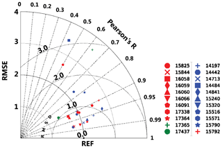
In addition, we have modified the method developed by Taylor (2001) for the purposes of summarizing model performance based on Pearson R, RMSE and RMSD, a measure of the pattern root-mean-square difference, given as follows:

$$\begin{array}{}\text{(1)}& \begin{array}{rl}\mathrm{RMSD}& =({\mathrm{RMSE}}^{\mathrm{2}}+{\mathrm{RMSE}}_{\mathrm{ref}}^{\mathrm{2}}-\mathrm{2}\cdot \mathrm{RMSE}\\ & \cdot {\mathrm{RMSE}}_{\mathrm{ref}}\cdot R{)}^{\mathrm{0.5}},\end{array}\end{array}$$

where RMSE is the root-mean-square difference of a test field, RMSE_ref is a root-mean-square difference of a reference field, and R is the correlation between test and reference fields (Taylor, 2001). In our modification, RMSE is the root-mean-square difference between simulations and observations, RMSE_ref is an acceptable measure of standard deviation between simulations and observations, and R is the correlation between simulations and observations. We selected a value of RMSE_ref=2.0 ^∘C as a reasonable measure based on a review of statistical measures found in other water temperature studies (Yearsley, 2012). The goal of our modification is to show how well the model results compare to the reference value for which the RMSE is 2.0 ^∘C and the correlation between simulations and observations is equal to 1.0.

3.4 Scenarios of watershed management

There can be significant impacts on streamflow and stream temperatures in watersheds where there is a transition from forested to urbanized lands and where there is development of watershed projects for water supply, flood control and generation of hydroelectric power. These are processes that have been ongoing in the Farmington River basin since the 18th century and are likely to continue. As a result, there will be a need for watershed planning and models such as the one we have developed that can provide support for these plans. The State of Connecticut's Department of Energy and Environmental Protection, in their Triennial Review of Water Quality Standards (CTDEEP, 2014), concluded that

The current temperature criteria in the WQS (Water Quality Standards) are insufficient to be protective of cold water aquatic life species. Temperature criteria should be revised to better align with fisheries management and restoration priorities of the state.

Beauchene et al. (2014) describe a stream classification system in Connecticut for fishes in three thermal classes, “Cold”, “Cool” and “Warm” that could be the basis for developing new water temperature criteria for the State of Connecticut's water quality standards. We compare water temperatures simulated with the DHSVM-RBM modeling system to the metrics from their classification system for selected scenarios of management actions. For this example, we consider the following four scenarios in the Farmington River basin that characterize maximum impacts for the riparian vegetation and watershed projects for water supply, flood control and generation of hydroelectric power:

• Scenario 1 (baseline). Simulated stream temperatures for the existing conditions for riparian vegetation and water storage projects.

• Scenario 2 (dam removal). Simulated stream temperatures for the existing conditions of riparian vegetation and no water storage projects.

• Scenario 3 (riparian removal). Simulated stream temperatures for the removal of all riparian vegetation with existing water storage projects remaining in place.

• Scenario 4 (dam and riparian removal). Simulated stream temperatures for the removal of both existing riparian vegetation and water storage projects.

4 Results

4.1 Hydrology

We simulated streamflows and the energy budget components with DHSVM for the Farmington River basin by estimating parameters in a manner similar to that described in previous studies (Cao et al., 2016; Meyer et al., 1997; Sun et al., 2015, 2016). Some parameters were estimated from available data sources including physiographic features of the basin. For others, we approached the problem by (1) choosing the range of parameter estimates from previous studies, and (2) varying a subset of parameters until a satisfactory measure of model performance, using the NSE, was met.

Table 4 USGS gage stations in the Farmington River basin (Fig. 1) and model performance evaluation criteria for daily and monthly flows simulated by DHSVM based on performance ratings from Moriasi et al. (2007). (VG – Very Good, G – Good, S – Satisfactory, U – Unsatisfactory.)

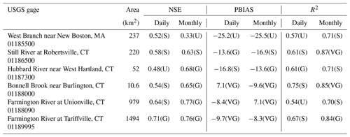
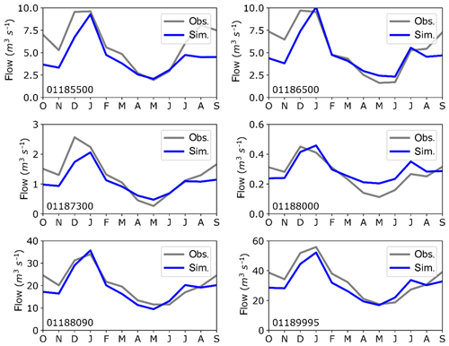
In our evaluation of DHSVM (Table 4; Figs. 3 and 4), we compare model results for both daily and monthly streamflows at six USGS gages distributed across the river network (Fig. 1), with the general performance ratings recommended in Table 3 of Moriasi et al. (2007). Although the parameters were calibrated to observed streamflows at USGS gage 01189995 near the basin outlet, the model performance at upstream gages is generally satisfactory. With the exception of daily flows at USGS gage 01187300 and monthly flows at USGS 01185500, both located in smaller tributaries, our results fall within the ratings of Satisfactory (S) to Very Good (VG), recommended in Moriasi et al. (2007). Model performance is best for the two gages with the greatest drainage area (USGS gage 01189995 and USGSG gage 01188090). We have also included the cumulative distribution function (CDF) for the daily flows as an additional metric for evaluating streamflow results. Overall, the CDFs at the two gaging stations with the greatest drainage characterize the distribution of flows better than for those gaging stations in the smaller tributaries, while the model performance in simulating the low flows is not as good as the higher flows in the smaller tributaries.

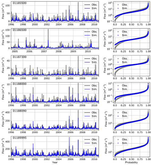
Figure 3 Time series and cumulative distribution function comparing simulated and observed daily stream flows at selected USGS gages in the Farmington River basin.

Figure 4 Time series comparing simulated and observed monthly-averaged stream flows at selected USGS gages in the Farmington River basin.

4.2 Stream temperature

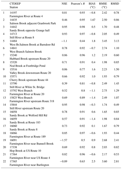
We obtained realizations of water temperature using the state estimates for the nominal solution (Supplement) in stream networks for the Farmington River basin. We accessed stream temperature data in 3-hourly times steps from the Spatial Hydro-Ecological Decision System (SHEDS, 2016) database at 22 monitoring sites (Fig. 1), made by the Connecticut Department of Energy and Environmental Protection (CTDEEP, 2014) for 3-hourly times steps in the Farmington River basin, with which to evaluate our simulation results. The period of available temperature observations varies by location. At some locations, the observations were collected for summer months only (e.g., CT-15320). Figure 5 presents the model evaluation at selected six CTDEEP sites, and Fig. S1 in the Supplement presents the model evaluation at the remaining 16 CTDEEP sites in the Farmington River basin. From this set of observations, we calculated the metrics for evaluating model performance based on the rationale described in Sect. 3.3, above. The statistical measures that characterize the stream temperature model performance at 3-hourly time steps are shown in Table 5 and the modified Taylor diagram for summarizing the degree to which the results cluster near the reference value is shown in Fig. 6.

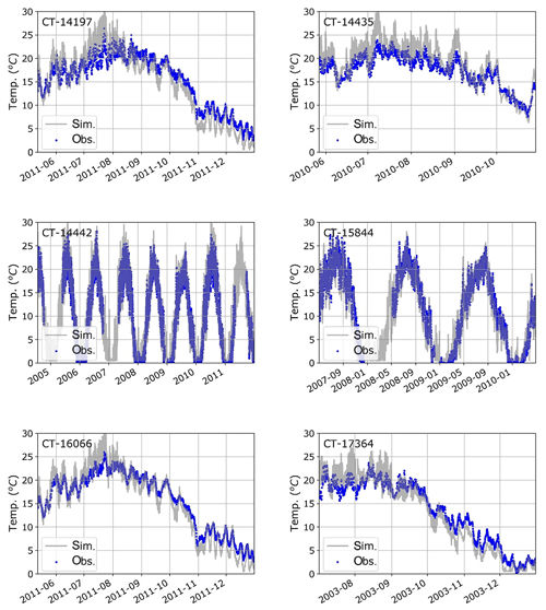
Figure 5 Time series comparing simulated and observed 3-hourly stream temperatures at six selected CTDEEP sites in the Farmington River basin. The period of available temperature observations varies by location.

Table 5 Statistical measures for comparison of daily-averaged simulated and observed water temperatures in the Farmington River.

Figure 6 Modified Taylor diagram (Taylor, 2001) summarizing model performance in terms of RMSE, Pearson R and centered RMSD. The point labeled “REF” represents a reference value for RMSE from Yearsley (2012).

4.3 Scenarios of watershed management

The four scenarios described in Sect. 3.4 provide an envelope of stream temperature outcomes for certain aspects of watershed management. We simulated stream temperatures in the Farmington River basin within the context of these scenarios. We use the results to examine (1) the difference in the stream temperature regime in streams between deep reservoirs and those without, and (2) the effect of watershed management on aquatic habitat.

To examine the effect of deep reservoirs on stream temperature, we used the simulations to estimate the average water temperature in the West Branch from its headwaters to the confluence with the Connecticut River for each month for the period 1996–2011. Figure 7 displays these results for the months of April, June, August and October with (Scenario 1) and without (Scenario 2) the major reservoirs, respectively, and also displays the available monthly-averaged CTDEEP observations for comparison with the actual data.

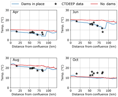
Figure 7 Monthly-averaged stream temperatures of April, June, August and October in the West Branch and main stem of the Farmington River for the following: dams in place – existing riparian shading and water management projects; no dams – removal of water management projects maintaining existing riparian shading; and monthly-averaged water temperatures at locations monitored by the Connecticut Department of Energy and Environment (CTDEEP).

We made use of the study by Beauchene et al. (2014) to examine the effect of watershed management on aquatic habitat. They defined three stream temperature metrics that classify streams in Connecticut as Cold, Cool, or Warm based on a comprehensive study of water temperature and fish communities in the rivers of Connecticut, including those in the Farmington River basin (Table 6). For each of the four management scenarios, we calculated the three metrics, June–August mean water temperature, July mean water temperature and maximum daily mean water temperature for the period 1996–2011. Based on the results, we estimated the manner in which each of the scenarios would affect thermal habitat for aquatic species throughout the Farmington River basin. We estimated the summer thermal thresholds of fish community transitions when two or more of the three conditions of Table 6 were met. This is similar to the approach used by Beauchene et al. (2014). The results are shown in Fig. 8a–d and Table 7.

Table 6 Stream temperature metrics (^∘C) for classifying streams in Connecticut into thermal classes (after Table 3 of Beauchene et al., 2014).

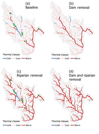
Figure 8 Thermal classes (Cold, Cool, and Warm) in the Farmington River basin using simulated results for (a) Scenario 1, (b) Scenario 2, (c) Scenario 3, and (d) Scenario 4 from Sect. 3.4. The green square in panels (a) and (c) indicate the location of the reservoirs.

Table 7 Percentage of watershed with Cold, Cool or Warm thermal class for watershed management scenarios described in Sect. 3.4. Metrics for estimating thermal classes are from Table 6 (following Beauchene et al., 2014).

We evaluated the impacts of modifications in hydrology and riparian vegetation using the metrics for the thermal classes associated with summer thermal thresholds of fish community transitions proposed by Beauchene et al. (2014). Model results showed that for the conditions of Scenario 1 (baseline) there are 57.7 km (7.7 %) of the Cold water thermal class, 586.8 km (78.4 %) of Cool water thermal class and 103.7 km (13.9 %) of Warm water stream thermal class in the Farmington River basin as well as primarily cool water habitat (84 %) with fewer segments of warm water (10 %) and cold water (6 %) habitats. In comparison, Beauchene et al. (2014) found that in the 160 sites in Connecticut they studied, 68.1 % could be characterized as cool water habitat. Since they do not report the percentages of stream segments with cold water or warm water habitat, there is no direct comparison with those habitat types, however. In addition, they limited their study to wadable streams only and did not include stream segments below dams, as we have.

In our assessment, model results for Scenario 2 indicated that removing the seven dams (Table 1) but maintaining the riparian vegetation would decrease the length of Cold water classes by 30.0 km and increase Warm water thermal classes by 34.1 km. The impacts on thermal classes would be felt primarily in the main stem of the Farmington River from Lake Colebrook downstream as far as Rainbow reservoir. Results from Scenario 2 also show the role reservoirs play in reducing the diurnal variations in stream temperature (Fig. 9).

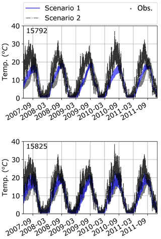
Figure 9 Simulated and observed water temperatures in the Farmington River downstream from West Branch reservoir (CTDEEP-15792 and CTDEEP 15825).

Removing the riparian vegetation while keeping the seven dams in place (Scenario 3) would have a significant impact on both Cold water and Cool water thermal classes. Cold water classes would be reduced by 31.3 km and Cool water classes by 359.0 km. Results showed that the impacts of removing riparian vegetation are systemic. They occur throughout the Farmington River watershed with the exception of 7.0 km of headwaters segments and 19.3 km below Lake Colebrook and West Branch reservoirs, the two reservoirs that release cold water from the hypolimnion. Removing both dams and riparian vegetation (Scenario 4) leaves only the 7.1 km of headwaters as Cold water habitat and results in an increase in the Warm water class to 531.4 km, compared to the 103.6 km results for Scenario 1 (Baseline).

5 Discussion

5.1 Hydrology

In our assessment of the impacts of hydrologic and land use alterations on water temperature in the Farmington River Basin we applied the distributed hydrologic model DHSVM for the purposes of estimating the hydrology for the four management scenarios of Sect. 3.4.

The water management projects we have included in our study (Table 1) modify the natural streamflow to varying degrees. For example, those that are primarily for the purposes of municipal water supply such as the Nepaug and the Barkhamsted Reservoirs that divert water are not accounted for in our analysis. Colebrook Lake is managed for flood control, hydroelectric power generation and riverflow augmentation for fisheries enhancement, all of which can modify the timing and amount of streamflow. The statistical metrics we calculated (Table 4) are for daily-averaged and monthly-averaged simulated unregulated streamflows for the 15-year period from 1996 through 2011. Nevertheless, the statistical metrics for the simulated unregulated flows at the two stream gages downstream from the major confluences (USGS gages 01188090 and 01189995) are comparable to those obtained in other applications of DHSVM (Cao et al., 2016) and the SWAT (Ficklin et al., 2012). With the exception of R² at USGS gage 01188090, the results can be characterized as varying from Satisfactory to Very Good using the recommendations of Moriasi et al. (2007). Future applications of DHSVM for river basins with reservoir that are regulated would benefit from adaptations to DHSVM such as those of Zhao et al. (2016).

5.2 Stream temperature

For the purposes of assessing the impacts of hydrologic and land use alterations on water temperature in the Farmington River watershed we have developed the nominal solution (Eqs. S5 and S6) for the linearized state-space water temperature model, RBM (Yearsley, 2009, 2012). The information required for complete development of the RBM model system is considerable and depends on the time and space scales that are to be modeled, as well as on the important physical processes that affect stream water temperatures in the basin. In addition, there are many processes that affect stream temperature which have received little or no study in the river basin. This includes the effects of groundwater return and hyporheic flow, conduction of heat through the stream bed and snowmelt (e.g., Evans et al., 1998; Kurylyk et al., 2016). The ability to incorporate these processes into the state space structure of RBM is limited to the number of available stream temperature monitoring sites. As a result, the number of degrees of freedom in the parameter space is simply too large to bound the problem with existing observations. Given the size of the parameter space and the limited number of stream temperature monitoring sites, we developed the RBM parameter space with the results from previous applications (Cao et al., 2016; Sun et al., 2015, 2016) and other studies (e.g., Boyd and Kasper, 2007; Chapra et al., 2008; Mohseni et al., 1998). Where possible, we used field observations and data that are readily available from multiple sources rather than from monitoring programs designed specifically for our purposes.

In our study, as well as others (Ficklin et al., 2014; van Vliet et al., 2012), the ability to test how well our approach leads to acceptable model results depends on the quality and quantity of observational data from publicly available sources. They are most often ones that are maintained by state and federal resource agencies. These are valuable sources of data; ones that are most often used to test and evaluate environmental models. However, the sampling design may not necessarily be one that is best suited for this purpose. As a result, there can be more uncertainty in applying these databases compared to studies for which monitoring programs are designed specifically for model development (e.g., Glose et al., 2017; Vatland et al., 2015).

For this study, we have estimated the metrics for model evaluation, described in Sect. 3.3, using 22 sites in the SHEDS database where the CTDEEP has archived observations of water temperature (Fig. 1). For the statistical measures in Table 5, the modified Taylor diagram (Fig. 6) provides a graphical way of summarizing the results in terms of Pearson R, RMSE and RMSD. These three metrics are referenced to a standard deviation (REF) of 2.0 ^∘C, corresponding to the estimated variance for the uncertainty analysis in Yearsley (2012). The clustering of points within the 2.0 ^∘C RMSD arc of the Taylor diagram correspond to those monitoring sites where model performance as measured by Pearson R and RMSE, is within the range of other studies (e.g., Beaufort et al., 2016; Du et al., 2018; Yearsley, 2012). The three monitoring sites in the Farmington River basin that are outside the 2.0 ^∘C RMSD arc (CT-14484, CT-16091, and CT-17365) have markedly lower values of standard deviation and correlation coefficient, as well as having negative values of NSE. These three sites are in locations with physical and hydrologic characteristics similar to the other 19 monitoring sites. Without more observations, it is difficult to conclude from the existing data why the simulations at these three sites differ markedly from the observed compared to the other sites.

The water temperature model, RBM, as developed here, has limitations for accurately simulating stream temperatures as streamflows become low. The contribution of bed conduction, nonpoint source inputs and hyporheic flows to the thermal energy budget becomes more important as stream depths and speeds become small (Boyd and Kasper, 2007; Kurylyk et al., 2016). In the DHSVM-RBM model system, we account for this condition by imposing minimum values on stream depths and speed rather than accounting for other depth-dependent process in the nominal solution (Eqs. S5 and S6). There are limitations of this approach for conditions of summer low flow periods in freely flowing stream segments of the Farmington River basin. This is evident in the simulated results shown in Fig. 5, which overestimate the diurnal variations at some monitoring sites (e.g., CT-14197, CT-14435, CT-16066, and CT-17364).

Important features of thermal thresholds in the Farmington River that emerge from our study include (1) the importance of headwater temperatures, (2) the impact of releases from deep reservoirs on downstream water temperatures, and (3) the role of riparian vegetation. The role of headwater temperatures in providing cold water habitat for stream fish assemblages is evident from the results for Scenarios 3 and 4. In the case of Scenario 3, for which riparian vegetation is removed, while dams are kept in place, the only cold water thermal classes remaining, other than below the two deep reservoirs that release water from the hypoliminion (Lake Colebrook and West Branch), are 7.1 km of headwaters stream segments. Similarly, these are the only Cold water segments remaining in Scenario 4, for which both dams and riparian vegetation are removed. Understanding the role of groundwater in headwater temperatures, although not directly considered in our study, would be important for preserving cold water habitat, especially during summer low flow.

By incorporating a two-layer reservoir model (Fig. 2) into the RBM model framework, we are able to capture certain important features of the water temperature regime downstream from the two deep reservoirs – Lake Colebrook Reservoir and West Branch Reservoir. Figure 9 illustrates the way in which the two-layer model simulates both the delay in timing of the maximum temperature and its magnitude, compared to the simulated results without the reservoirs. Furthermore, there is also a noticeable reduction in the magnitude of the diurnal variations, a feature associated with the thermal inertia of the large volume of water that is a characteristic of both river-run and deep reservoirs.

The longitudinal distribution of monthly-averaged stream temperatures in the West Branch of the Farmington River (Fig. 7) tells a similar story regarding the impact of the deep reservoirs. The impact on stream temperature downstream of reservoirs which have long residence times and the capability for storing and releasing water from the hypolimnion is evident for the segment of the river below the Lake Colebrook–Hogback series of reservoirs (∼ River KM 60–95). For the months of April, June and August, the effect of the reservoirs is to provide cooling of stream temperatures for this segment of the river. The results for October (Fig. 7, Oct) do indicate, however, that the two-layer representation of the reservoirs does not entirely capture the delayed heating effects that are associated with reservoir operations. This may be due to the simplified approach to stream hydrology we have implemented for the Farmington River system (i.e., natural flow without regulation). This is most likely to be important in the hydrologic and thermal dynamics for the Lake Colebrook–Hogback series of reservoirs. A major function of Lake Colebrook is flood control and the reservoir is generally drafted in late summer and fall, increasing the ratio of heated surface area to volume of the reservoir during this period. In addition, the state-space formulation of the reservoir model (Eqs. S13a and b) does not include vertical eddy diffusion of thermal energy, as is the case for other similar approaches, such as that of Niemeyer et al. (2018). In future applications, further model refinement in this regard is necessary to improve model performance.

6 Conclusions

Our goals in this research were (1) develop nominal solutions for state-space estimates of streamflow and water temperature based on first principles, results of previous studies and data available from publicly available sources, and (2) provide examples of the way in which the models might be applied to watershed management.

Our development of a nominal solution for obtaining state estimates of streamflow and stream temperature has many similarities to other approaches formulated in terms of conservation laws. However, we believe it differs conceptually from others by acknowledging the uncertainty, as well as providing a more general paradigm for environmental models, whether they have been characterized as “data-driven/statistical” or “deterministic/process-based'.

We have parameterized the hydrologic model, DHSVM, and the stream temperature model, RBM, with data from publicly available sources and taken advantage of the mature status of stream temperature modeling based on the conservation laws of mass, momentum and energy. It is encouraging that when we test our models with available observation, our approach results in metrics that are within the range of similar studies. By obtaining the nominal solutions for streamflow and stream temperature, we have addressed previous concerns regarding the lack of available information for model development by accessing publicly available data and making use of previous research. There is room for improvement, of course, and it is important to emphasize that maintenance and updating of these databases and monitoring programs is essential.

We have presented an example of the way in which these methods can be used for evaluating watershed management decisions. Our approach to the characterization of aquatic habitat based on simulated thermal classes (Fig. 8a–d) should be viewed, first of all, in terms of its potential as a decision support system. Given the robust performance of DHSVM-RBM for the Farmington River basin, the outcomes we have presented provide basic insights into the impacts of land use management on aquatic habitat.