the Creative Commons Attribution 4.0 License.
the Creative Commons Attribution 4.0 License.
 | 25 Oct 2019
Hydrodynamic simulation of the effects of stable in-channel large wood on the flood hydrographs of a low mountain range creek, Ore Mountains, Germany
Daniel Rasche
Christian Reinhardt-Imjela
Achim Schulte
Robert Wenzel
Large wood (LW) can alter the hydromorphological and hydraulic characteristics of rivers and streams and may act positively on a river's ecology by i.e. leading to increased habitat availability. On the contrary, floating as well as stable LW is a potential threat for anthropogenic goods and infrastructure during flood events. Concerning the contradiction of potential risks and positive ecological impacts, addressing the physical effects of stable large wood is highly important. Hydrodynamic models offer the possibility of investigating the hydraulic effects of anchored large wood. However, the work and time involved varies between approaches that incorporate large wood in hydrodynamic models. In this study, a two-dimensional hydraulic model is set up for a mountain creek to simulate the hydraulic effects of stable LW and to compare multiple methods of accounting for LW-induced roughness. LW is implemented by changing in-channel roughness coefficients and by adding topographic elements to the model; this is carried out in order to determine which method most accurately simulates observed hydrographs and to provide guidance for future hydrodynamic modelling of stable large wood with two-dimensional models.
The study area comprises a 282 m long reach of the Ullersdorfer Teichbächel, a creek in the Ore Mountains (south-eastern Germany). Discharge time series from field experiments allow for a validation of the model outputs with field observations with and without stable LW. We iterate in-channel roughness coefficients to best fit the mean simulated and observed flood hydrographs with and without LW at the downstream reach outlet. As an alternative approach for modelling LW-induced effects, we use simplified discrete topographic elements representing individual LW elements in the channel.
In general, the simulations reveal a high goodness of fit between the observed flood hydrographs and the model results without and with stable in-channel LW. The best fit of the simulation and mean observed hydrograph with in-channel LW can be obtained when increasing in-channel roughness coefficients throughout the reach instead of an increase at LW positions only. The best fit in terms of the hydrograph's general shape can be achieved by integrating discrete elements into the calculation mesh. The results illustrate that the mean observed hydrograph can be satisfactorily modelled using an adjustment of roughness coefficients.
In conclusion, a time-consuming and work-intensive mesh manipulation is suitable for analysing the more detailed effects of stable LW on a small spatio-temporal scale where high precision is required. In contrast, the reach-wise adjustment of in-channel roughness coefficients seems to provide similarly accurate results on the reach scale and, thus, could be helpful for practical applications of model-based impact assessments of stable LW on flood hydrographs of small streams and rivers.
- Article
(8583 KB) - Full-text XML
- BibTeX
- EndNote


Large wood (LW) is a natural structural element of rivers and streams with forested catchments (Gurnell et al., 2002; Roni et al., 2015). It is part of the permanently produced amount of plant detritus in terrestrial ecosystems before it enters rivers and surrounding riparian areas (Wohl, 2015). In fluvial systems, large wood can be defined as dead organic matter with a woody texture that has a diameter of at least 0.1 m (Kail and Gerhard, 2003). Unlike in the above-mentioned definition of Kail and Gerhard (2003), several studies have also included a length for large wood – at least 1 m – for distinction (i.e. Gurnell et al., 2002; Andreoli et al., 2007; Comiti et al., 2008; Bocchiola, 2011; Kramer and Wohl, 2017; Wohl, 2017). The latter definition is adapted in the present study.
Large wood influences the physical structure of watercourses as it increases streambed heterogeneity by forming scour pools (Abbe and Montogomery, 1996), causing sediment sorting and altering the water depth as well as flow velocity (Pilotto et al., 2014). Hence, the presence of large wood can lead to increased habitat availability in rivers and streams (Wohl, 2017). Positive ecological impacts of LW on fish species (i.e. Kail et al., 2007; Roni et al., 2015) and the macro-invertebrate fauna (i.e. Seidel and Mutz, 2012; Pilotto et al., 2014; Roni et al., 2015) have been documented. A recent review of the hydromorphological and ecological effects of LW with a focus on river restoration can be found in Grabowski et al. (2019).
In stream restoration projects, the presence of large wood can result in rapid hydromorphological improvements (Kail et al., 2007). Consequently, wood placement has a high potential with respect to stream restoration measures (Kail and Hering, 2005); this is particularly true in countries such as Germany where many watercourses lack high hydromorphological diversity (BMUB/UBA, 2016).
Large wood assemblages and elements are more likely to be stable when their length exceeds the channel width (i.e. Gurnell et al., 2002); this is most likely to occur in small first-order streams and rivers, which in turn are the most abundant order of water courses on the planet (Downing et al., 2012). However, even in small but steep headwater streams, large wood may be transported during hydrogeomorphic events of high magnitude such as debris flows (Galia et al., 2018) or extreme floods. A conceptual model for a first estimate of large wood transport in water courses is given in Kramer and Wohl (2017), including hydrological and morphological variables. Further detailed information regarding large wood dynamics in river networks can be found in recent reviews by Ruiz-Villanueva et al. (2016a) and Wohl (2017). Large wood may drift during floods, and elements jam at bridges or other infrastructure and cause increased water levels, damage or completely destroy anthropogenic goods and structures (Schmocker and Hager, 2011). On the contrary, stable large wood reduces water conveyance (Wenzel et al., 2014) and leads to increased water levels upstream and, in turn, increased risk of flooding and water logging in surrounding areas. For these reasons, as well as to ensure navigability in larger rivers (Young, 1991), LW has been removed from European rivers and streams for more than a century (Wohl, 2015). As a result, the usage of LW in river restoration in the form of leaving naturally transported wood in watercourses or the placement of artificial stable wood is a controversial topic (Roni et al., 2015; Wohl, 2017).
Due to the opposing considerations of the potential risks of large wood for anthropogenic goods and structures on the one hand and high ecological benefits on the other hand, it may be necessary to distinguish river sections in which large wood can remain or be introduced from those where it needs to be removed (Wohl, 2017). Large-wood-related segmentation of rivers and streams requires knowledge of the physical effects caused by mobile and stable in-channel large wood. Although several studies have addressed the general hydraulic impact of LW in field studies (i.e. Daniels and Rhoads, 2004, 2007; Wenzel et al., 2014), laboratory experiments (i.e. Young, 1991; Davidson and Eaton, 2013; Bennett et al., 2015) and reviews (i.e., Gippel, 1995; Montgomery et al., 2003) regarding the alteration of water level, flow pattern, flow velocity and discharge, a project and site specific examination is necessary to evaluate the local consequences of intended stream restoration measures.
The resulting physical effects of stable in-channel LW (Smith et al., 2011) as well as the mobility, transport and deposition of large wood (i.e. Ruiz-Villanueva et al., 2014; Ruiz-Villanueva et al., 2016b) can be addressed using numerical hydrodynamic models. Numerical hydrodynamic models for the simulation of open-channel hydraulics can be classified by their dimension and solve the shallow water equations (SWE) in their one-, two- or three-dimensional form for simulating channel flow in just one (x) direction (one-dimensional), horizontally resolved (x and y directions) but depth-averaged (two-dimensional) or fully resolved (in the x, y and z directions) (Liu, 2014). Due to i.e. the increasing work and computational time involved with increasing dimension, the applicability of one-, two- or three-dimensional models depends on the scale and phenomena of interest (Liu, 2014). For simulating the general hydraulic behaviour on the reach scale, two-dimensional models are useful tools (Liu, 2014). A detailed description of the different model types and examples of application can be found in Liu (2014) or Tonina and Jorde (2013) with a focus on ecohydraulics. Several studies have considered stable large wood in the scope of one- and two-dimensional hydrodynamic simulations, to investigate, for example, its influence on flood hydrographs (Thomas and Nisbet, 2012) or floodplain connectivity (Keys et al., 2018), or have considered stable LW in research applications with an ecological focus by investigating its impact on habitat availability or suitability (i.e. He et al., 2009; Hafs et al., 2014). In addition, Lange et al. (2015) simulated the effect of roughness elements including stable LW in the scope of stream restoration analyses. Regarding the hydraulic impact of stable large wood on flood hydrographs, Thomas and Nisbet (2012) simulated large wood to delay flood passage but no attenuation of peak discharge was modelled. Similar effects of stable LW on flood hydrographs were investigated by Wenzel et al. (2014) in field experiments, where a delay and a narrower shape via a transformation from higher to lower discharges, but only a minor attenuation of the average flood hydrograph was observed. Furthermore, representing and integrating large wood elements in hydrodynamic models has been addressed in different studies using three-dimensional hydrodynamic models (i.e. Smith et al., 2011; Allen and Smith, 2012; Lai and Bandrowski, 2014; Xu and Liu, 2017). However, the modelling approach applied varies with studies. As an extensive review of applicable numerical hydrodynamic modelling systems and approaches for simulating large wood is beyond the scope of the present study, a recent overview with a focus on LW dynamics as well as the representation of large wood and vegetation in simulations can be found in Bertoldi and Ruiz-Villanueva (2017).
Despite the necessity for a discrete representation of stable large wood elements in the calculation mesh of hydrodynamic models to obtain accurate results (Smith et al., 2011), and as conducted in different studies (i.e. Hafs et al., 2014; Lange et al., 2015; Keys et al., 2018), LW elements are often accounted for using roughness coefficients in hydrodynamic model applications (Smith et al., 2011). The impact of large wood on in-channel roughness has been investigated by Gregory et al. (1985), Shields and Smith (1992), Shields and Gippel (1995), Dudley et al. (1998), MacFarlane and Wohl, (2003) and Wilcox and Wohl (2006). In addition, Curran and Wohl (2003) and Wilcox et al. (2006) have studied its partial contribution to channel roughness coefficients. However, a methodological lack remains in quantitatively estimating LW-related changes of in-channel roughness coefficients (Wohl, 2017), especially under field conditions (Wilcox et al., 2006). The large-wood-induced alteration of channel roughness coefficients and overall hydraulic impacts such as backwater effects, as investigated by Schalko et al. (2019) for instance, are crucial for the identification of local risks. Therefore, remaining knowledge gaps in these fields lead to uncertainties regarding the use large wood in river restoration and natural flood risk management in practice (Grabowski et al., 2019) and may hamper its application. Against this background, the aim of the present study is to simulate the physical effects of stable in-channel LW elements on flood hydrographs in a creek reach in low mountain ranges using a two-dimensional hydrodynamic model and previously conducted field experiments, which are explicitly described in Wenzel et al. (2014). The field data offer the rare opportunity to validate simulated large-wood-related hydraulic effects on hydrographs of small flood events. By conducting different hydrodynamic simulations, we aim (1) to quantify the change of channel roughness coefficients in the entire channel or at LW positions, which is necessary to obtain the most accurate model results of flood hydrographs with stable large wood elements in the channel. As discrete LW elements are required for the most accurate model results (Smith et al., 2011), we aim (2) to compare previous model results with simulations with discrete large wood elements created by manipulating the calculation mesh. However, the integration of discrete elements into the calculation mesh can be highly time- and work-intensive (Lai and Bandrowski, 2014), which becomes especially true for larger-scale applications. Hence, a comparison of the simulation accuracy between incorporating large wood via a rather quick change of channel roughness coefficients and as time-demanding simplified mesh elements could provide beneficial information for future studies simulating stable large-wood-related effects on stream hydraulics and ecology.
Although limited to smaller streams and rivers where large wood jams and elements can be assumed to be stable or situations in which large wood elements are anchored, the present study can contribute to the ability of predicting hydraulic impacts of stable in-channel large wood within hydrodynamic simulations; it can also provide beneficial practical information for conducting simulation-based impact assessments of stream restoration projects considering stable large wood by comparing different methods of large wood roughness modelling.
The study reach comprises a 282 m long section of the Ullersdorfer Teichbächel, which is a small first-order headwater creek located in the Ore Mountains in south-eastern Germany. The catchment of the Ullersdorfer Teichbächel (50∘36′48.52′′ N, 13∘15′51.24′′ E, WGS84) covers an area of 1.8 km2 and drains into the Elbe River via several higher-order tributaries including the Schwarze Pockau, the Flöha, the Zschopau and the Mulde.
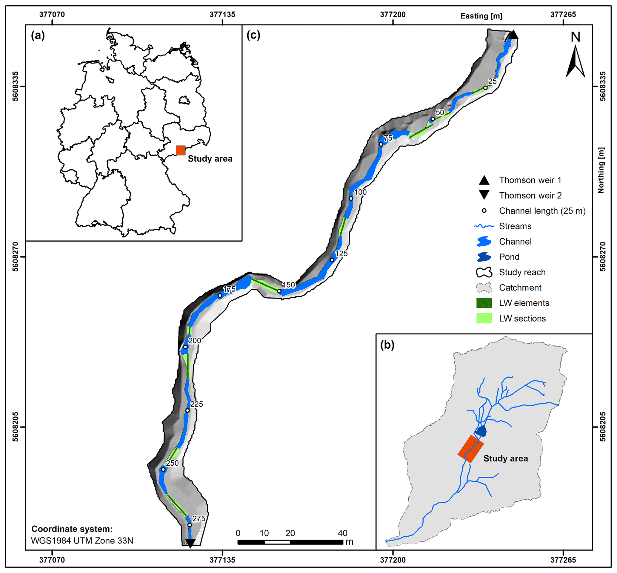
Figure 1(a) Location of the study area in Germany (administrative units: BKG, 2018) and (b) the position of the study reach in the catchment of the Ullersdorfer Teichbächel (stream network: LVA, 2002). (c) LW-affected sections and positions of discrete LW elements in the study reach.
The study reach is located in the centre of the catchment, approximately 50 m downstream of an artificial rafting pond built in the 16th century. Two Thomson weirs mark the study reach's upper and lower limits at elevations of 754.1 and 744.5 m a.s.l. (Fig. 1), resulting in a difference in elevation of 10.4 m and an average channel gradient of 3.7 %. Channel dimensions vary strongly along the study reach, i.e. the channel width ranges from <0.8 to 2 m. Similarly, a high variability of stream bed grain sizes can be detected (Fig. 2). Moderately steep sections with a sand- and fine-gravel-dominated bed structure alternate, with reach sections of higher gradients dominated by coarse gravel, cobbles and small boulders with sizes of up to 0.3 m in diameter. The boulders consist of gneiss varieties representing the dominant bed rock formations in the catchment. Beside a highly variable stream width, alternating slope gradients and grain sizes lead to an alternation of stream depth along the study reach and, hence, a generally complex channel structure.
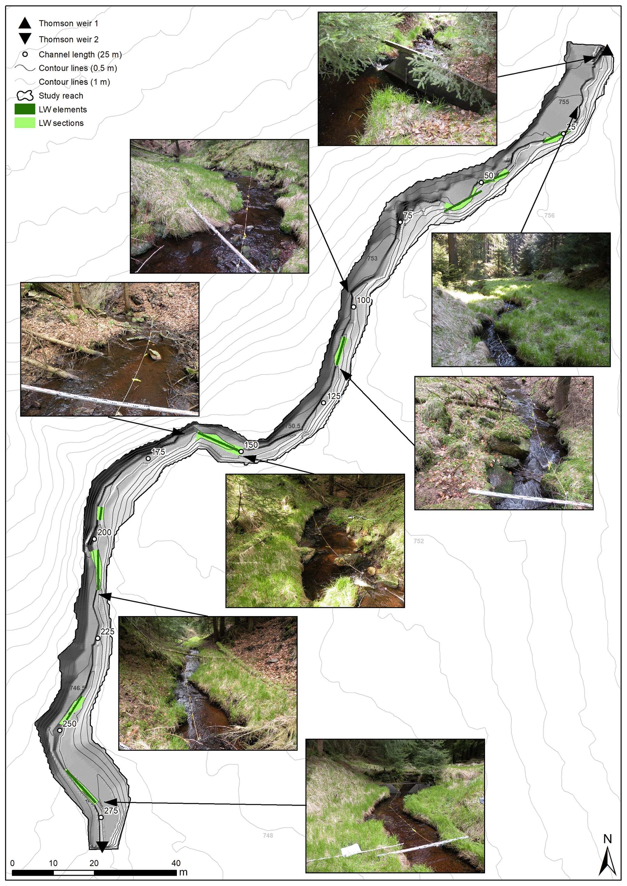
Figure 2Detailed map of the study reach (topographic data outside reach: GeoSN, 2008). Photographs were taken 9 years after the field experiments in May 2017 in the direction of flow (north to south).
The overall morphological character along the 282 m study reach consists of riffle–pool sequences in moderately steep sections as well as step–pool morphologies along sections with smaller channel widths and larger in-channel boulders (Fig. 2). In the latter, channel-spanning steps with corresponding hydraulic jumps and eroded pools were observed in May 2017.
The majority of the catchment of the Ullersdorfer Teichbächel is covered with coniferous forest on prevailing Cambisols and Podzols including scattered deciduous trees. The dominating species is spruce (Picea abies) with the occasional occurrence of mountain pines (Pinus mugo) and beech trees (Fagus sylvatica) (Wenzel et al., 2014). Trees occur sporadically in the narrow floodplain along the channel of the study reach with grassy vegetation on fluvic Gleysols covering most parts. However, smaller floodplain sections are covered with bare soil or leaf litter. Perpendicular to the direction of flow, the maximum width of the floodplain measured from channel banks varies between 7 and 0 m, when channel banks immediately change into the embankments confining the study reach.
At the nearest gauging station Zöblitz, which is located approximately 13 km downstream the catchment's outlet at the Schwarze Pockau River and drains an area of 125 km2, the mean annual discharge is 2.29 m3 s−1. If the value is extrapolated using a regional analysis based on drainage areas, the mean discharge at the outlet of the study reach is 16 m3 s−1. The flow regime of the study area is dominated by snowmelt that generates high flows in March and April (gauge Zöblitz, period 1937 to 2015; LfULG, 2017a). Floods of low to medium magnitudes are generated by intense snowmelt and rainfall on snow in spring or by storm events in summer. Larger flood events are caused exclusively by summer storms (Petrow et al., 2007), but the flood magnitudes are strongly influenced by land use and are greatly affected by past forest changes (Reinhardt-Imjela et al., 2018).
3.1 The HYDRO_AS-2D hydrodynamic model
In this study, the two-dimensional HYDRO_AS-2D (version 2.2) hydrodynamic model is used to simulate the flow in the study reach with and without LW. HYDRO_AS-2D was developed for practical applications in water management (Nujić, 2006) and has been used in several studies simulating flow conditions in river sections for flood risk management (i.e. Rieger and Disse, 2013) or with an ecological focus (i.e. Lange et al., 2015); HYDRO_AS-2D can produce a higher goodness of fit than other two-dimensional models as shown, for example, in Lavoie and Mahdi (2017). Especially in southern Germany and Austria, HYDRO_AS-2D has become a standard two-dimensional modelling system for hydrodynamic model applications (Faber et al., 2012). Due to the numerical approaches used in the modelling system, HYDRO_AS-2D is capable of simulating mass exchange between channel and forelands, streams comprising hydraulic jumps, steep channel sections and a high variability of channel width as well as dike breaches (Nujić, 2006). The latter is to some extent comparable with the rapid release of water initiated by opening the flap gate weir used in the field experiments (see Sect. 3.2). For the above-named reasons, HYDRO_AS-2D was chosen for the present study.
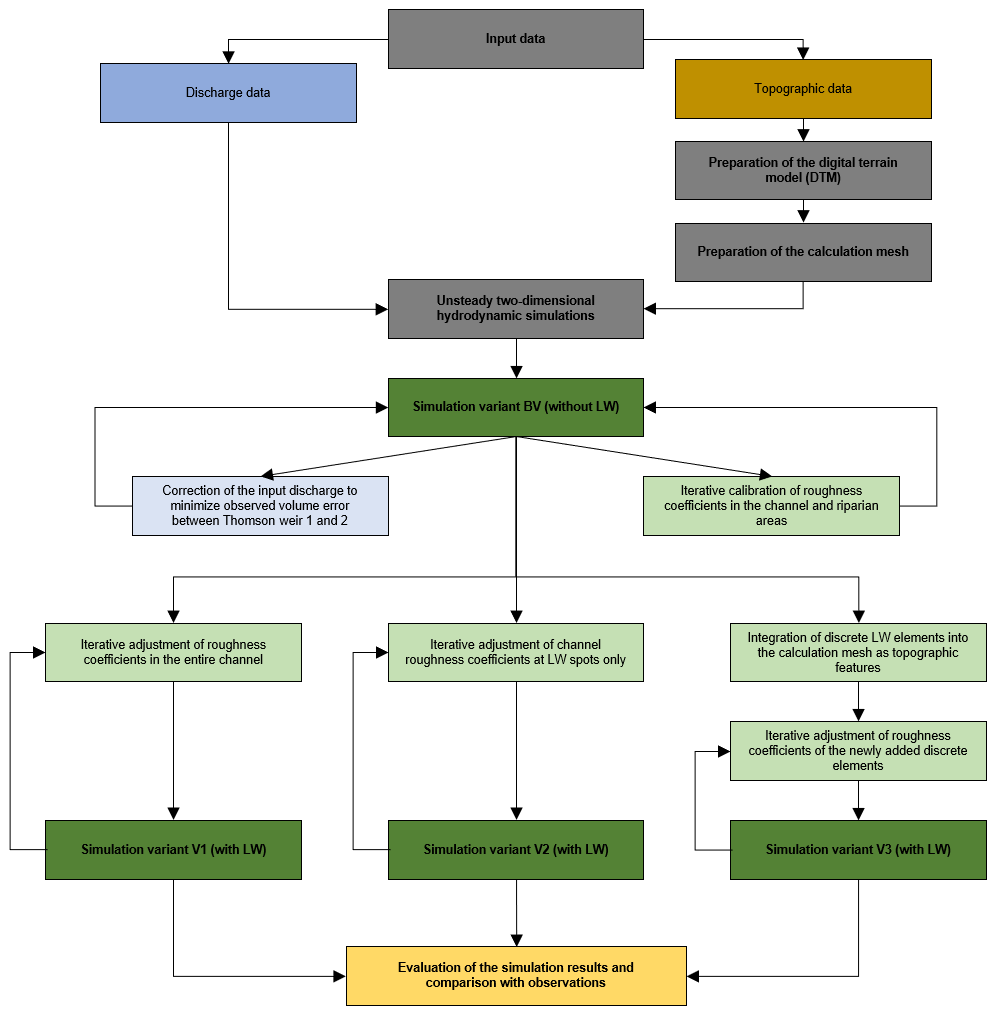
HYDRO_AS-2D solves the two-dimensional shallow water equations (SWE) at each node of a linear calculation mesh composed of quadrilateral and triangular elements of different sizes, representing a digital terrain model of the channel and the forelands. Shallow water equations are solved using finite volume approximations for spatial discretion, while time is discretized using second-order Runge–Kutta methods (Nujić, 2006). Water flow is computed through all sides of the control volume around each node using different order polynomials and upwind schemes (Nujić, 2006). Surface roughness is represented by Strickler coefficients defined for each element of the calculation mesh. Similarly, local viscosity can be defined for each mesh element. Mesh generation, preprocessing, the setting of model boundary conditions and simulation result visualization of HYDRO_AS-2D v2.2 are conducted using the Surface-water Modeling System (SMS) v10.1 (Aquaveo Inc., USA) software. An overview of the methodological procedure described in the following sections can be found in Fig. 3.
3.2 Datasets and mesh generation
The presented study is based on data previously collected during field experiments in March 2008 (Wenzel et al., 2014) in the river section under investigation. In this earlier study, the pond upstream the experimental reach was dammed using a flap gate weir and multiple flood waves of equal magnitude (return period of 3.5 years) were generated. The first eight experimental runs were conducted with nine large wood elements (spruce tree tops with lengths ranging from 3 to 11.5 m and a mean length of 8.5 m), which were placed and fastened in the channel lengthwise 9 months earlier. After the experimental runs with LW, all LW elements were removed and 12 additional flood waves were generated without the trees. During all experimental runs, water levels were continuously recorded with a temporal resolution of 1 s at the beginning and end of the river section using Thomson weirs equipped with pressure gauges. For each Thomson weir, the averaged (mean) hydrographs of experimental runs with and without LW were calculated and used as the upper model boundary condition (Thomson weir 1) and for the validation of model outputs (lower boundary condition, Thomson weir 2), respectively.
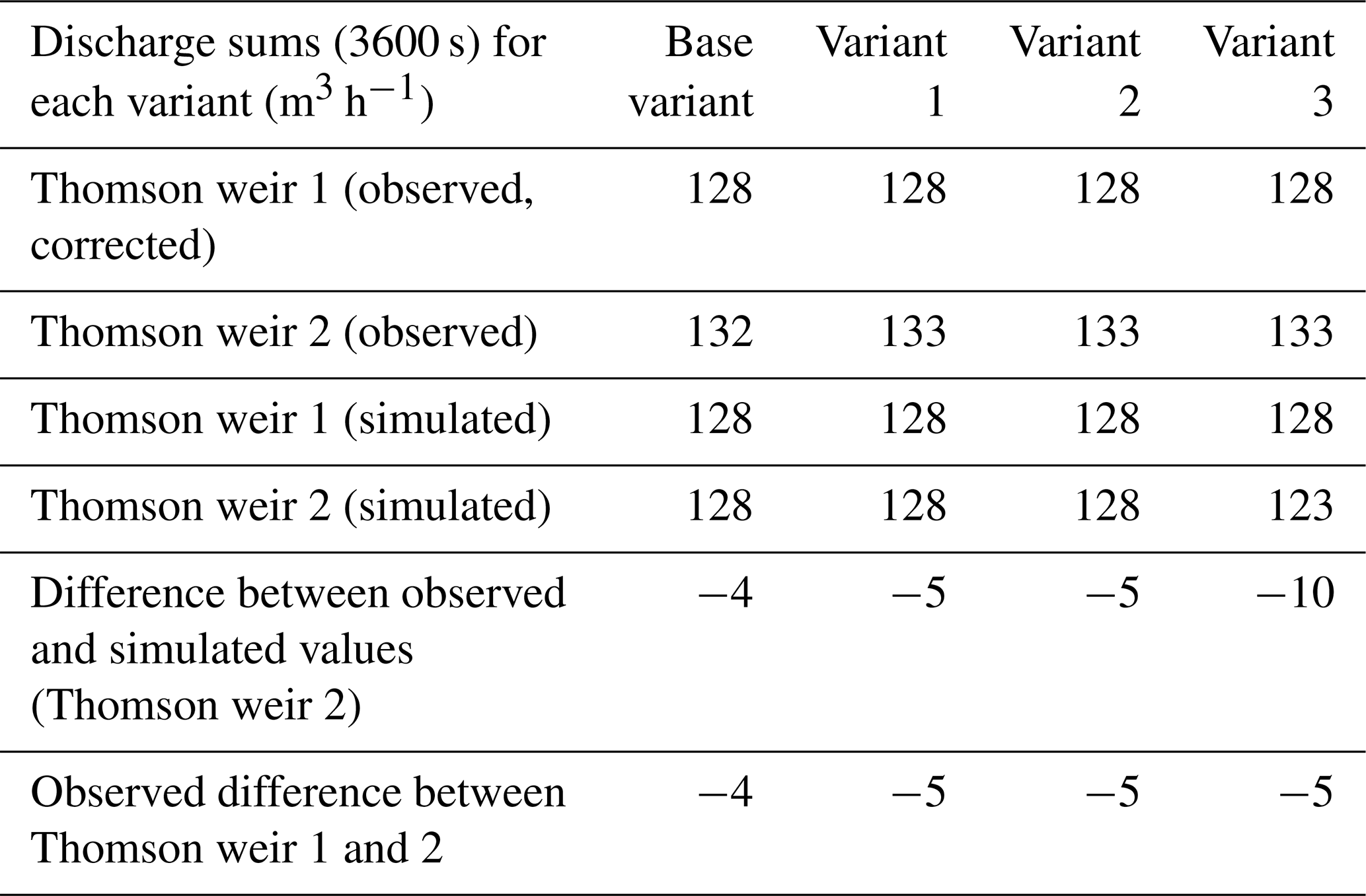
During the development of the hydraulic model, a measurement error was detected in the water level measurement at Thomson weir 1 (input weir), which results in a significantly lower discharge volume at Thomson weir 2, although larger water inflows between both weirs were not observed in the field. The measurement error of the input weir was corrected by increasing water levels in the original water level time series of the pressure gauge and recalculating discharge. The measured water levels at the first weir had to be increased by a maximum of 0.024 m until the total flood volume at both weirs was nearly equal (Table 1).
Table 1Average observed and simulated discharge sums (m3 h−1) at both Thomson weirs for all simulation variants. For variant V1 and V2 discharge sums with subsequent adjustment of riparian Strickler coefficients are displayed.
To generate a digital terrain model (DTM) for the river section studied, data from a cross-sectional geodetic survey conducted with a Spectra Precision AB Geodimeter 400 in 2008 were available. To improve the implementation of the channel in the hydrodynamic model, the channel width was surveyed again in intervals of 5 m using a measuring stick in May 2017. Furthermore, a digital elevation model with a spatial resolution of 2 m ×2 m (Saxon State Office of Geoinformation and Surveying, 2008) was used for better reproduction of the floodplain morphology. The final DTM for the model was generated from processing and combining all topographic datasets in the ArcGIS v10.5 (ESRI Inc., USA) software environment and creating a triangular irregular network (TIN) before transforming it into a raster dataset. The resulting DTM was exported as equally spaced elevation points with a spatial resolution of approximately 0.5 m ×0.5 m for the entire study reach including riparian areas and embankments. From the point grid, the calculation mesh required for simulations with HYDRO_AS-2D was created. Mesh generation was carried out in the SMS v10.1 software environment and according to mesh quality requirements of HYDRO_AS-2D, such as minimum and maximum angle of mesh elements or maximum number of element connections per node (Nujić, 2006). The calculation mesh was composed of quadrilateral and triangular elements. In the channel of the study reach, quadrilateral elements were created by stepwise mesh generation between surveyed cross-sectional point elevation profiles via linear interpolation of elevation between profiles. A triangular mesh was generated in the riparian areas and along embankments by using equally spaced elevation points. After merging quadrilateral channel elements and triangular foreland elements as well as including additional topographic features to the calculation mesh (Fig. 4) to match field observations, roughness coefficients were assigned to each mesh element. The Strickler coefficients kst were estimated for channel sections with similar bed material and the floodplain during field surveys in May 2017 with reference to established roughness coefficient classifications for different land cover and surface material types (i.e. Chow, 1959) as well as in accordance with observed ground cover during field experiments in 2008.
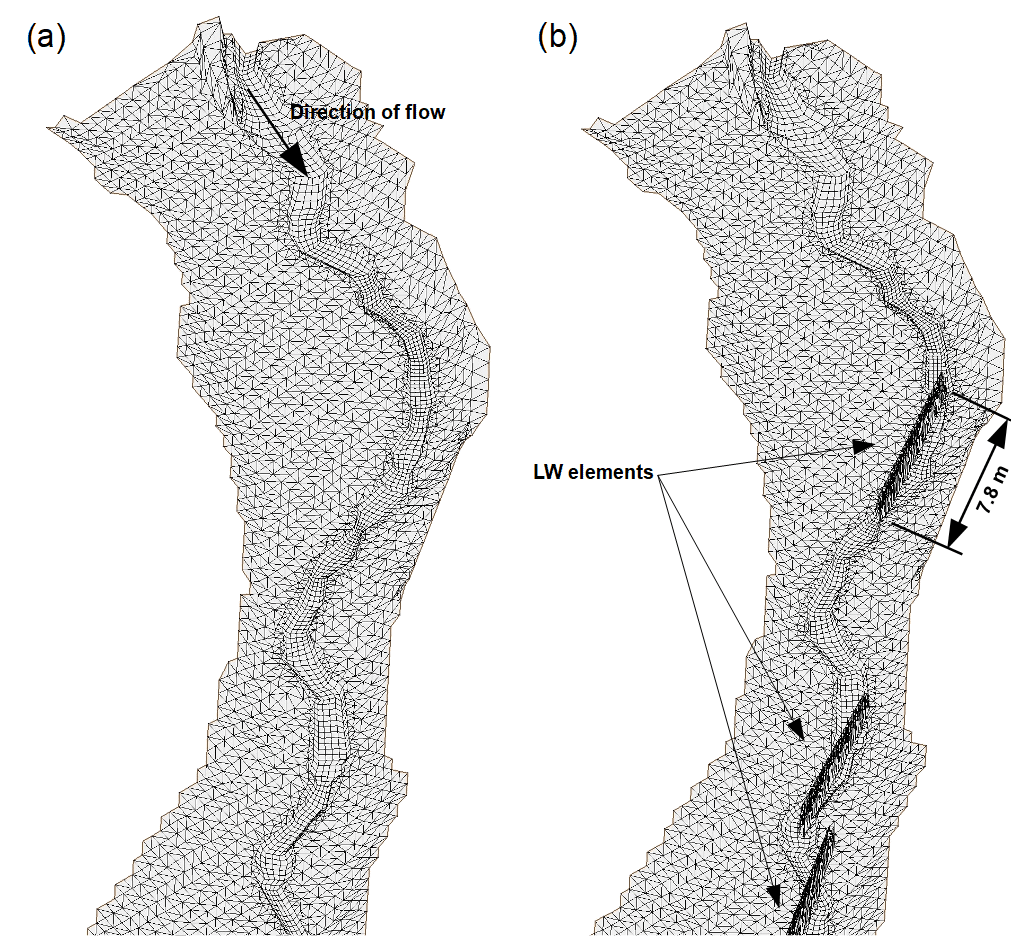
Figure 4(a) Calculation mesh of the hydrodynamic model used in simulation variants RV, V1 and V2 with the use of variable Strickler coefficients adjusted for the entire channel (V1) or adjusted at the positions of all LW elements only (V2); (b) mesh with discrete LW elements used in variant V3. Example of the first 60 m of the study reach.
3.3 Hydrodynamic modelling
Boundary conditions for the unsteady hydrodynamic simulations are defined in SMS v10.1. For flow simulations of the experimental reach without LW, the averaged discharge time series without LW at Thomson weir 1 (Fig. 5) is defined as the water inflow into the study reach. Water influx is defined at the location of Thomson weir 1 in the calculation mesh, represented by the uppermost cross-sectional nodestring in the channel. For the simulations with in-channel LW, the averaged time series with LW at Thomson weir 1 (Fig. 5) is used as the system input.

Figure 5Average measured and corrected flood hydrographs observed during field experiments with and without stable in-channel large wood at both Thomson weirs (after Wenzel et al., 2014).
For the simulations without and with LW, the inflow hydrographs at Thomson weir 1 are extended forward by 5400 s using the first discharge value of the corrected mean experimental hydrograph without and with LW. This is done to achieve field conditions of minor flow through the channel in the study reach before the experimental flood waves enter the channel. This results in a total simulation time of 9000 s for each simulation with and without LW with a temporal resolution of 1 s.
Simulation results are obtained at the location of Thomson weir 2 in the calculation mesh represented by the lowermost cross-sectional nodestring in the channel of the study reach. Model performance is assessed by visual comparison of mean observed and simulated flood hydrographs without and with LW at Thomson weir 2 as well as by calculating the statistical goodness of fit parameters, the Nash–Sutcliffe efficiency (NSE), the percent bias (PBIAS) and the RSR (ratio of the root-mean-square error to the standard deviation of observed values) using the hydroGOF package by Zambrano-Bigiarini (2017) in R (R Core Team, 2017). For NSE a value of 1 indicates the highest model accuracy, whereas the optimum value for RSR and PBIAS is 0 (Moriasi et al., 2007).
3.4 Hydrodynamic simulation variants
In the scope of this study, four different simulation variants are applied to investigate the effects of in-channel large wood on flood hydrographs in a small low mountain stream: (1) the reference variant RV representing the simulation of field experiments without in-channel LW and (2–4) variants V1 to V3 for simulating field experiments with LW.
Variant RV is used to obtain the best fit of the mean observed and simulated hydrograph without LW at Thomson weir 2 by iteratively adjusting Strickler roughness coefficients in the channel and in riparian areas. In the reference variant and all other simulation variants calibration is performed to achieve the best possible simulation of the moment of rise, the rising limb and the peak discharge of the mean observed hydrograph at Thomson weir 2. Calibrated roughness coefficients leading to the best fit in variant RV will be used as initial roughness coefficients in the calculation mesh of variants V1, V2 and V3.
Variant V1 represents the first simulation with LW. Calibrated Strickler coefficients from variant RV are iteratively adjusted for the entire channel (integrated roughness). Adjustments are made percent-wise and with equal magnitude to enable the equal scaling of spatially varying roughness coefficients of mesh elements in the channel. This approach was included because the integrated channel roughness of a river section is an important input parameter for rainfall–runoff models at the mesoscale or of larger watersheds, which often only use one Strickler (or Manning) coefficient per section.
Similarly, roughness is scaled in variant V2, in which Strickler coefficients from variant RV are adjusted at the positions of all LW elements only. LW element locations and corresponding LW-influenced channel sections (length of each LW element) are derived from Wenzel et al. (2014). For each channel section roughness coefficients are adjusted percent-wise and with equal magnitude.
In contrast to variants V1 and V2, where LW is represented by the reach-wise and section-wise adjustment of Strickler coefficients of quadrilateral in-channel calculation mesh elements, variant V3 includes the integration of simplified discrete roughness elements by manipulating the existing calculation mesh used in variant RV. Therefore, discrete elements with the maximum stem length and width (without branches) of each individual LW are incorporated into the calculation mesh by creating corresponding rectangular polygons overlying the mesh. Polygons are positioned in order to have the largest possible part located in the channel of the study reach. Based on the existing calculation mesh, new mesh nodes are positioned at 0.2 m intervals along polygon boundaries and within a 0.1 m distance outside polygons. Nodes along polygon boundaries receive the elevation of the closest upstream non-LW node increased by 1.5 m. The elevation of nodes within a 0.1 m distance is interpolated from the existing calculation mesh. As mesh quality requirements (see Sect. 3.2) need to be maintained, positions of some added nodes are slightly shifted. Additional quadrilateral and triangular mesh elements are created between nodes added to the mesh. All newly created mesh elements representing discrete LW elements (Fig. 4) are parameterized with the same Strickler coefficient in order to retrieve the best fit between the simulated and mean observed hydrograph with LW at Thomson weir 2. Strickler coefficients of mesh elements representing discrete large wood elements are used to account for i.e. branches of real spruce tree tops implemented into the channel during the field experiments. Coefficients are determined iteratively during the calibration of simulation variant V3.
4.1 Simulation variant RV
In the reference variant, the best fit in the unsteady hydrodynamic simulation without LW was achieved with in-channel Strickler coefficients ranging from 6 m1∕3 s−1 for channel sections with larger boulders to 12 m1∕3 s−1 in channel sections where fine gravel forms the stream bed. A Strickler coefficient of 3.5 m1∕3 s−1 was defined for riparian areas during calibration. The distribution of calibrated Strickler coefficients in the study reach of all simulation variants can be found in Fig. 6.
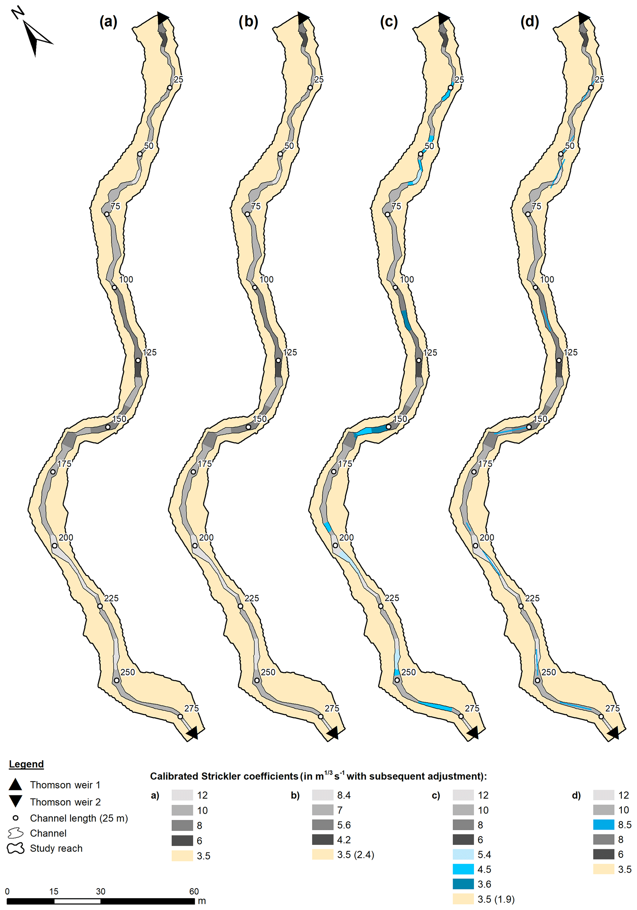
Figure 6Distribution of calibrated roughness coefficients of all simulation variants with and without LW in the study reach: (a) reference variant RV without LW, (b) variant V1 with stable LW as an increase of roughness in the entire channel, (c) variant V2 with stable LW as an increase of roughness at element positions only and (d) variant V3 with LW as discrete topographic elements of the calculation mesh. If displayed, values in parentheses represent the Strickler coefficient after subsequent adjustment.
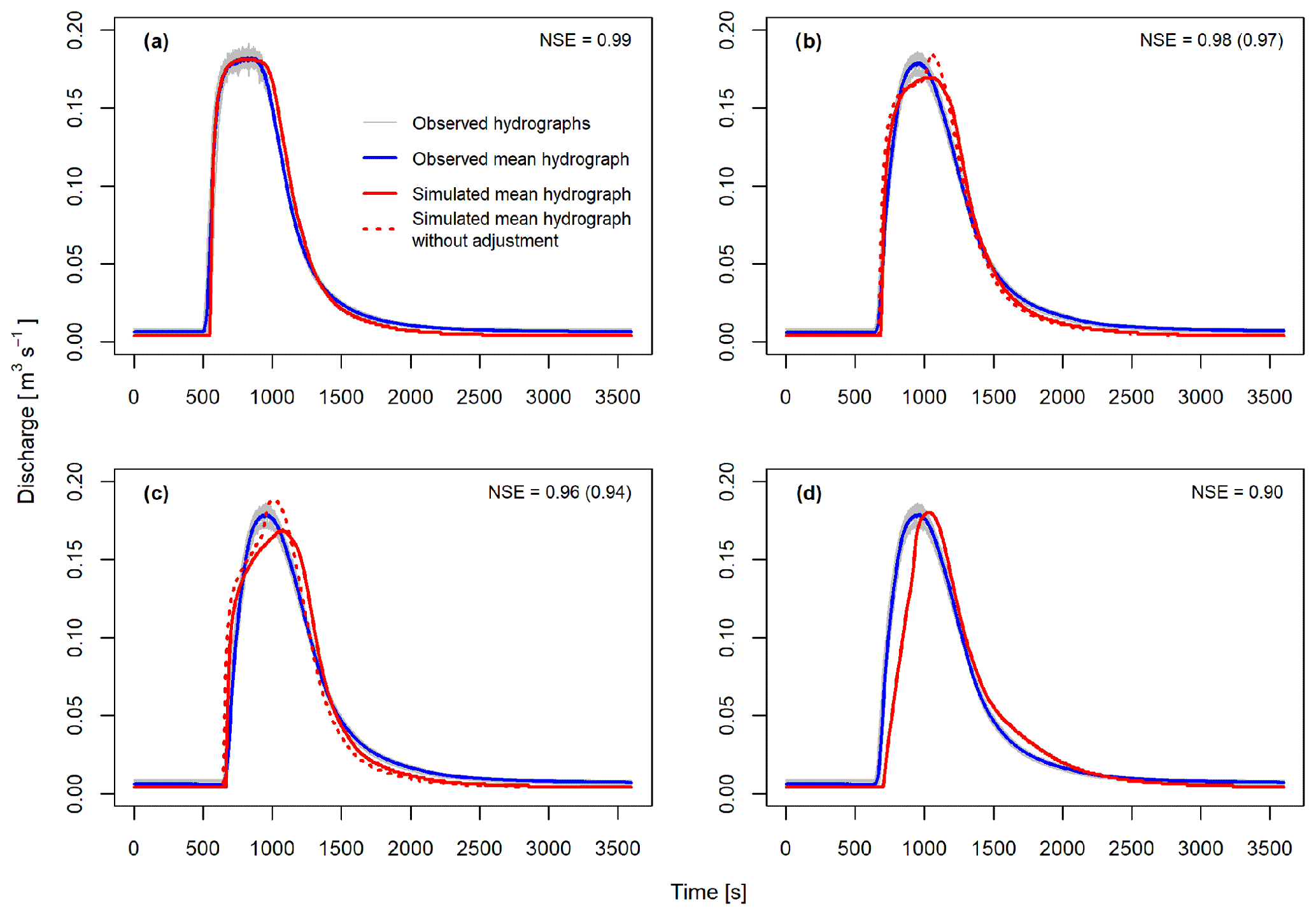
Figure 7Best simulated mean flood hydrographs of all simulation variants with and without LW at Thomson weir 2: (a) results of the reference variant RV without LW, (b) variant V1 with stable LW as an increase of roughness in the entire channel, (c) variant V2 with stable LW as an increase of roughness at element positions only and (d) variant V3 with LW as discrete topographic elements of the calculation mesh. For simulation variants V1 and V2 the best fit with and without subsequent adjustment of riparian Strickler coefficients is displayed. The Nash–Sutcliffe efficiency (NSE) is shown for each simulation variant. If displayed, values in parentheses represent the NSE of simulations without adjustment of riparian roughness coefficients.
Table 2Calculated statistical goodness of fit parameters for all simulation variants. For variant V1 and V2 goodness of fit parameters with and without subsequent adjustment of riparian Strickler coefficients are displayed.
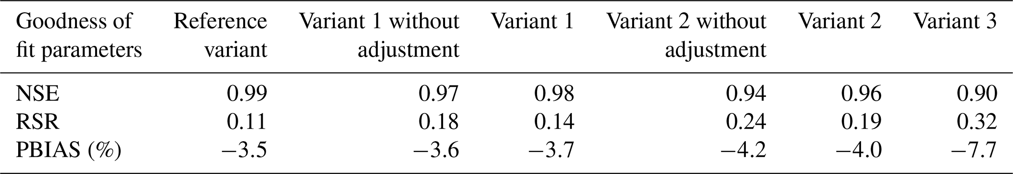
Observed and simulated hydrographs of the simulation are shown in Fig. 7. In general, the model closely simulates the characteristics of the observed hydrograph. Only the crest is slightly wider in the model and a slight model underestimation can be observed at the beginning and in the second half of the simulation period. The good model performance is reflected by a high NSE of 0.99 as well as a low RSR (0.11) and PBIAS (−3.5 %). The statistical goodness of fit parameters of all simulation variants are summarized in Table 2. The cumulative maximum inundated area comprises 739 m2, which is defined as the total area of mesh elements inundated during simulation.
4.2 Simulation variant V1 – integrated increase of roughness in the channel
In the first simulation variant V1 of field experiments with in-channel large wood, Strickler coefficients were decreased in the entire channel based on the coefficients of the simulation without large wood (variant RV). A decrease of Strickler values and, hence, an increase of roughness of 30 % in the entire channel resulted in the best fit between the mean observed and simulated hydrograph. Consequently, in-channel Strickler coefficients range from 4.2 to 8.4 m1∕3 s−1 in variant V1 (Fig. 6). The nine LW elements in the field investigations cover 75.1 m of the 282 m long channel reach, i.e. the simulated 30 % increase of the integrated channel roughness refers to a LW percentage of 27 % of the channel length.
The resulting simulated hydrograph of variant V1 shows a good representation of the time of rise as well as the rising limb of the observed hydrograph (Fig. 7). However, in the peak discharge phase the simulated hydrograph does not rise continuously until peak values are reached. If the Strickler coefficients in the channel foreland (riparian area) are decreased from 3.5 to 2.4 m1∕3 s−1 in addition to the channel roughness, the break in the crest of the hydrograph disappears (see Sect. 5.2). After adjusting roughness coefficients in riparian areas, the rising limb and peak phase of the observed hydrograph are represented slightly better. Nevertheless, discharge values during the peak phase show a distinct underestimation of the observed values. Similarly, differences can be found along the falling limb between the observed and simulated values. The maximum inundated area comprises 861 m2 before and 880 m2 after riparian roughness adjustment. Nash–Sutcliffe efficiency values of 0.97 before and 0.98 after the adjustment of roughness coefficients in riparian areas were achieved. The RSR shows values of 0.18 and 0.14 before and after adjustment, respectively, while PBIAS slightly increases after adjustment from −3.6 % to −3.7 %. (Table 2).
4.3 Simulation variant V2 – increase of roughness in LW sections
In simulation variant V2, in-channel roughness coefficients derived from variant RV were altered in large-wood-affected channel sections only. Here, a reduction of Strickler coefficients of 55 % resulted in the best fit of observed and simulated hydrographs. Depending on the LW-affected channel section, Strickler coefficients between 3.6 and 5.4 m1∕3 s−1 were derived (Fig. 6). The resulting simulated hydrograph properly represents the time of rise. Compared with variant V1, the rising limb is less accurately modelled. Similarly to variant V1, a discontinuous peak phase is generated in the simulations. Again, an increase of the roughness in riparian areas is necessary to simulate a hydrograph with a more realistic, continuous rise of discharge up to the crest of the hydrograph. Strickler coefficients in riparian forelands were reduced from 3.5 to 1.9 m1∕3 s−1. In addition, both simulated hydrographs (with and without subsequent adjustment of riparian roughness coefficients) show an overestimation of the observed discharge along the falling limb of the flood wave, whereas a distinct underestimation can be observed during the peak phase as well as at the beginning and the end of the experiments (Fig. 7). Before adjusting riparian surface roughness, the maximum cumulative inundation area is 859 m2. After subsequent adjustment inundated area rises to 892 m2. NSE values range from 0.94 before to 0.96 after adjusting riparian Strickler coefficients, while the RSR decreased from 0.24 to 0.19 and the PBIAS from −4.2 to −4.0 (Table 2). With respect to the general shape of simulated hydrographs as well as the statistical model performance assessment, variant V1 reveals a better representation of the observed hydrograph of the field experiments with in-channel large wood.
4.4 Simulation variant V3 – implementation of LW as discrete elements
In the last simulation variant (V3), large wood is integrated into the model as simplified discrete elements by manipulating the calculation mesh. The created mesh elements representing discrete LW elements received a Strickler coefficient of 8.5 m1∕3 s−1 to account for branches and in order to obtain the best fit between mean observed and simulated hydrograph (Fig. 6). As shown in Fig. 7, the simulated hydrograph rises slightly later than the mean observed hydrograph, which results in differences between the simulated and observed values along the falling limb. Additionally, a slight overestimation of peak discharges can be observed as well as the underestimation of discharges at the beginning and end of the simulation. The maximum water-covered area comprises 927 m2 and is much larger than in previous simulation variants. Statistical goodness of fit parameters show an NSE value of 0.90, a RSR value of 0.32 and a PBIAS of −7.7 %. Especially the PBIAS of variant V3 is much higher than in all other simulation variants (Table 2). According to the classification of Moriasi et al. (2007), goodness of fit parameter values calculated for variant V3 as well as for all other simulation variants in this study indicate highly accurate simulation results. Despite the temporal shift between the average simulated and observed flood hydrograph as well as the lower goodness of fit according to the classification of Moriasi et al. (2007), the general narrow shape of the flood hydrograph of the field experiments with in-channel LW is most accurately modelled in variant V3.
5.1 Simulations of flood hydrographs in the investigated creek section
In general, the two-dimensional hydrodynamic model closely mimics the flow conditions of the field experiments without LW (variant RV). Especially the time of rise, the rising limb and the flood peak are accurately represented, and minor deviations can be observed along the hydrograph's falling limb only due to the broader shape of the simulated hydrograph. However, it has to be noted that measurement errors may also occur in the field data, as demonstrated by the fact that the input time series measured at Thomson weir 1 had to be corrected to reduce the volume error between both weirs. After the correction, the cumulated volume error between both weirs was reduced to 4 m3 h−1 without LW and 5 m3 h−1 for the field experiments with LW (1 m3 s−1) (Table 1). The remaining difference between both weirs lies in the range of what can be estimated as natural water influx between both weirs based on runoff per square kilometre estimations from regional analyses of the nearest gauging station for the days of the field experiments (LfULG, 2017b). Depending on the spatial resolution of the DTM used for calculation (2 and 5 m), the average water influx ranges from 3 to 6 m3 h−1. Hence, the remaining volumetric difference can be attributed to diffuse lateral water influx during the runtime of each experiment and is likely to be responsible for the modelled (Fig. 7) and observed (Fig. 5) lower discharges before and after flood passage at Thomson weir 2. However, after correction it can be assumed that the measured data are a reliable reference for the hydrodynamic simulation.
The broader shape of the simulated hydrograph is likely to have been caused by the calculation mesh used, representing the terrain surface. The calculation mesh is based on topographic field data gathered in the scope of the field experiments in 2008 to find the most suitable locations to position large wood elements (Wenzel et al., 2014). Therefore, small topographic features in the channel and adjacent riparian areas are not included in the elevation dataset and, hence, in the calculation mesh. This especially applies to step–pool sequences in the study reach. Steps and pools produce rapid flow energy losses caused by corresponding hydraulic jumps and result in a deceleration of flow (Wilcox et al., 2011), where the amount of energy loss dynamically depends on water level (Comiti et al., 2009). Furthermore, erosion and transport of bed material leads to flow energy losses (Yen, 2002). As such features are missing in the calculation mesh, roughness coefficients are used to account for their impact on water flow. However, calibrating in-channel roughness coefficients may lead to a much more continuous decrease of flow velocities instead of intense, punctual flow decelerations with implications for downstream flow conditions; this, in turn, results in a broader peak of the simulated flood hydrograph. These issues illustrate the necessity for a high-resolution calculation mesh that includes small-scale topographic features in the channel and microtopography in riparian areas to obtain accurate model results.
Despite the discrepancies described above, the simulation of variant RV shows a very precise simulation of the observed hydrograph of the field experiments without large wood, which is also indicated by the statistical goodness of fit parameters revealing a very high model accuracy according to the classification of Moriasi et al. (2007). Hence, averaged flood hydrographs of the field experiments without large wood can be accurately simulated using the model set-up, illustrating its applicability for simulating the flow conditions in the study reach.
5.2 Simulating the hydraulic impact of stable in-channel LW using roughness coefficients
In simulation variants V1 and V2, roughness coefficients are used to represent large wood in the study reach. Both variants show a correct simulation of the time of rise of the flood hydrograph. Differences occur along the rising limb as well as the hydrograph's peak. Here, variant V1 produces a better fitting hydrograph. Compared with the simulation result of the mean observed hydrograph of the field experiments without in-channel LW, variants V1 and V2 produce less closely fitting simulated hydrographs, which is also indicated by the slightly lower values of statistical goodness of fit parameters. Nevertheless, these values still indicate a very high model accuracy, suggesting that a less time-consuming adjustment of roughness coefficients allows for an accurate simulation of stable large-wood-induced hydraulic effects.
In-channel LW elements decelerate flow beyond their own dimensions by generating upstream backwater areas and downstream wake fields of substantial length (i.e. Young, 1991; Bennett et al., 2015). Such features were also observed during field experiments (Wenzel et al., 2014). This means that LW affects flow upstream and downstream in an area that is larger than the wood piece itself, which could be one reason for the slightly better simulation results in V1 compared with V2.
For both simulation variants, the subsequent adjustment of riparian roughness coefficients is necessary to improve the goodness of fit. Only increasing riparian roughness by decreasing Strickler coefficients results in a smooth crest as it can be originally observed in the field experiments. As the calibrated roughness coefficients from the simulation without large wood are the baseline roughness for the simulations with wood, the riparian-zone roughness coefficients are calibrated to the flood extent of the conditions without large wood. Due to generally higher water levels in the field experiments and in the simulations with large wood, more water flows through a larger riparian area covered with vegetation. In the model, water flows too fast through adjacent riparian areas without subsequent adjustment of roughness. Emerged rigid elements such as riparian vegetation can lead to an increase of the Manning n roughness coefficient and, hence, a decrease of Strickler coefficients due to increasing friction exerted on flow (Shields et al., 2017). Therefore, a larger wetted area with generally low flow depths, a largely continuous cover of dense grassy vegetation and an uneven microtopography, due to i.e. elevated grass root wads observed in adjacent riparian areas during field experiments, could have led to the necessity to increase local roughness in this study – especially due to the lack of such features in the model's calculation mesh.
Decreasing Strickler coefficients by 30 % in variant V1 and 55 % in LW-affected sections only (V2) are in the range of previous studies. For instance, Gregory et al. (1985) detected a LW-related increase in the Manning n roughness coefficient of 48.5 % and Dudley et al. (1998) show an average increase of 36 %. Furthermore, MacFarlane and Wohl (2003) compare streams with and without LW and find the Darcy–Weisbach f to be 58 % higher on average in streams containing in-channel LW. However, it should be noted that boundary conditions, such as discharge, river size, LW volume, and so on, as well as the methodological approaches greatly vary between studies. For example, MacFarlane and Wohl (2003) investigate high-gradient mountain streams, whereas Shields and Gippel (1995) focus on lowland rivers. This illustrates the need for a common framework to better compare studies on large wood, as previously proposed by Wohl et al. (2010). This becomes especially true regarding the influence of stable in-channel LW on roughness coefficients.
The results presented may only be valid for small, single-thread and steep rivers with a defined amount of stable large wood elements which indicates the narrow boundary conditions of this study. When modelling the potential impact of stable large wood as a change of in-channel roughness coefficients with different boundary conditions and without data on large-wood-influenced discharge for calibration, the application of ensemble simulations with literature-based values of large-wood-induced increase of roughness may be used for a first assessment. Here, estimation methods for large-wood-induced roughness increase in small, high-gradient streams and rivers such as that previously developed by Shields and Gippel (1995) for large lowland rivers would be useful. Additionally, reviews of recent advances in research on the hydraulics of LW in fluvial systems would be highly beneficial, similar to recent reviews and meta-analyses addressing ecological implications (i.e. Roni et al., 2015), large wood dynamics (i.e. Ruiz-Villanueva et al., 2016a; Kramer and Wohl, 2017), related risks for anthropogenic infrastructure (i.e. De Cicco et al., 2018) and large wood in fluvial systems in general (Wohl, 2017).
5.3 Representation of in-channel LW as discrete elements
Simulation variant V3 generates the best simulated hydrograph with regard to its overall shape compared to the mean observed hydrograph of field experiments with LW, indicating the best simulation of flow processes in the study reach. Therefore, the time-consuming incorporation of discrete elements is an appropriate starting point for an advancement of model implementation and further studies on the hydrodynamics of in-channel LW. However, variant V3 produces a temporal shift between the mean simulated and observed flood hydrograph, causing a slightly delayed rise and falling limb of the flood hydrograph and, hence, a delayed passage of the flood wave at Thomson weir 2. Natural discrete LW elements have a complex shape, which strongly varies from piece to piece (and over time) concerning their geometry with twigs, branches, needles and floating debris caught up in the twigs. This complex shape and the permeability of LW elements and jams cannot be implemented in depth-averaged hydrodynamic models in detail and have to be simplified. The simplified implementation in terms of element impermeability, dimensions and the position of wood pieces may result in overly strong flow alterations, which, in turn, lead to higher amounts of water being retained in the study reach and, thus, the temporal shift of the modelled hydrograph. Intense flow alterations may also account for the fact that a subsequent adjustment of riparian roughness coefficients is not required in variant V3, as overly strong energy losses and flow declarations caused by discrete LW objects account for roughness originally caused by other roughness elements not represented in the calculation mesh (such as riparian vegetation and microtopography).
Nevertheless, variant V3 still shows a very high goodness of fit. A similarly high Nash–Sutcliffe efficiency was obtained in the study of Keys et al. (2018), who use discrete weirs to represent large wood objects and simulate their effects on floodplain connectivity. However, although variant V3 reveals the best simulation result, the temporal shift results in a lower goodness of fit and, hence, model quality compared with simulation variants V1 and V2. Therefore, solely relying on statistical goodness of fit indicators on such a high spatio-temporal scale may not be sufficient, and visual interpretation should not be excluded when assessing model results.
Although the roughness coefficient approach presented in this study is feasible with all models that are based on the SWE, only models enabling the simulation of two- and three-dimensional flow conditions can be used for the incorporation of simplified discrete large wood elements. In this study, only a single design of discrete large wood elements was incorporated as topographic features into the calculation mesh. Other designs may be also suitable, such as discrete weirs (Keys et al., 2018) or arrays of pillars that allow water to flow through. Thus, further research, including a comparison of different designs of discrete large wood elements in two-dimensional simulations under equal boundary conditions, could be beneficial. Furthermore, in the present study, calibration is solely conducted using the hydrograph at Thomson weir 2. As point measurements of flow depth, velocity and inundation extent in the field could improve model accuracy assessments, multi-criteria calibration approaches may be considered in future studies simulating the hydraulic effects of stable in-channel large wood.
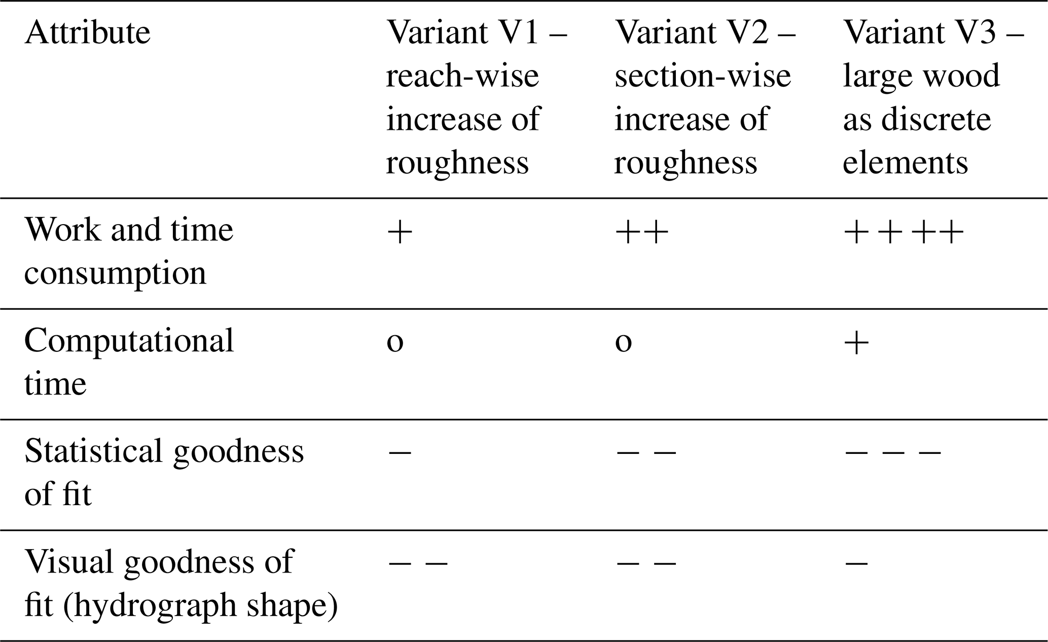
The hydrodynamic simulations conducted in the present study show that average flood hydrographs of previously conducted field experiments without in-channel LW can be accurately simulated in the small and high-gradient study reach using HYDRO_AS-2D. Nevertheless, minor discrepancies need to be considered. The effect of stable in-channel LW was satisfactorily simulated using roughness coefficients. However, differences in model quality can be detected between increasing in-channel roughness in the entire reach or in LW-affected channel sections only, where the latter results in a lower statistical goodness of fit. Visually, most accurate simulations of LW-related impacts on flood hydrographs regarding its overall shape can be obtained using discrete large wood elements as proposed in previous studies (Smith et al., 2011); however, this comes with a temporal shift between observation and simulation values due to the impermeability of the LW elements as well as higher effort and time requirements regarding their incorporation into the model (Table 3). Therefore, using channel roughness coefficients to simulate the impact of stable large wood elements on discharge time series seems to be similarly accurate to the implementation of discrete elements on the reach or larger (i.e. catchment) scale, where minor differences are smaller than the overall model uncertainty. Although constrained to the boundary conditions of this study, the simulation results indicate that the impact of stable in-channel large wood may be simulated with a reduced amount of time and work required for the model set-up and incorporation of discrete large wood elements via the use of roughness coefficients. Thus, model-based impact assessments of, for instance, stream restoration measures considering stable large wood, may become more feasible; this is especially true on the larger scale or in less critical channel-sections, where a fully resolved flow assessment with three-dimensional models is not required or practical. However, the present study is restricted to narrow boundary conditions, which, in turn, illustrates the need for further research comparing methods of stable large wood incorporation in different models with varying model dimensions and boundary conditions regarding channel morphology, large wood characteristics and water flow. Nevertheless, by comparing methods for simulating the impact of stable large wood on the reach scale, the present study can provide helpful information for practical applications in modelling stable large-wood-related effects in small, first-order streams and rivers.
Table 3Attributes of approaches for large wood implementation applied in this study relative to the reference variant without large wood. Signs indicate that an attribute is higher (+), lower (−) or equal to (o) the simulation without stable large wood.
Discharge time series (hydrographs) with and without large wood at both Thomson weirs used for the simulations and other related data are available upon request from the corresponding author.
DR carried out the data preprocessing, analyses and hydrodynamic modelling, prepared the paper and revised the paper during the review process. CRI provided the idea for this study, undertook project conceptualization and supervision of the underlying thesis, assisted with data processing, modelling and paper preparation, as well as review of the paper prior to initial submission and throughout the review process. AS was the supervisor of the underlying thesis and reviewed the paper prior to the initial submission and throughout the review process. RW provided experimental data and expertise regarding the field experiments and reviewed of the paper prior initial submission.
The authors declare that they have no conflict of interest.
We acknowledge support from the Open Access Publication Initiative of Freie Universität Berlin.
This paper was edited by Matjaz Mikos and reviewed by Bruno Mazzorana, Daniel Scott and two anonymous referees.
Abbe, T. B. and Montgomery, D. R.: Large woody debris jams, channel hydraulics and habitat formation in large rivers, Regul. River., 12, 201–221, https://doi.org/10.1002/(SICI)1099-1646(199603)12:2/3<201::AID-RRR390>3.0.CO;2-A, 1996.
Allen, J. B. and Smith, D. L.: Characterizing the impact of geometric simplification on large woody debris using CFD, Int. J. Hyd. Eng., 1, 1–14, https://doi.org/10.5923/j.ijhe.20120102.01, 2012.
Andreoli, A., Comiti, F., and Lenzi, M. A.: Characteristics, distribution and geomorphic role of large woody debris in a mountain stream of the Chilean Andes, Earth Surf. Proc. Land., 32, 1675–1692, https://doi.org/10.1002/esp.1593, 2007.
Bennett, S. J., Ghaneeizad, S. M., Gallisdorfer, M. S., Cai, D., Atkinson, J. F., Simon, A., and Langendoen, E. J.: Flow, turbulence, and drag associated with engineered log jams in a fixed-bed experimental channel, Geomorphology, 248, 172–184, https://doi.org/10.1016/j.geomorph.2015.07.046, 2015.
Bertoldi, W. and Ruiz-Villanueva, V.: Physical and numerical modelling of large wood and vegetation in rivers, edited by: Tsutsumi, D. and Laronne, J. B., Gravel-bed rivers: Processes and disasters, West Sussex, 729–753, https://doi.org/10.1002/9781118971437.ch27, 2017.
BKG – German Federal Office for Cartography and Geodesy (Ed.): German administrative units ATKIS-VG2500, scale 1:2,500,000, available at: http://www.geodatenzentrum.de/geodaten/gdz_rahmen.gdz_div&gdz_spr=deu&gdz_akt_zeile=5&gdz_anz_zeile=1&gdz_unt_zeile=19&gdz_user_id=0, last access: 24 February 2018.
BMUB/UBA – German Federal Ministry for Environment, Environmental Protection, Construction and Nuclear Safety/German Federal Office for the Environment: Die Wasserrahmenrichtlinie – Deutschlands Gewässer 2015, Bonn, Dessau, 2016.
Bocchiola, D.: Hydraulic characteristics and habitat stability in presence of woody debris: A flume experiment, Adv. Water Res., 34, 1304–1319, https://doi.org/10.1016/j.advwatres.2011.06.011, 2011.
Chow, V. T.: Open-channel hydraulics, Tokyo, Japan, 1959.
Comiti, F., Andreoli, A., Mao, L., and Lenzi, M. A.: Wood storage in three mountain streams of the Southern Andes and its hydro-morphological effects, Earth Surf. Proc. Land., 33, 244–262, https://doi.org/10.1002/esp.1541, 2008.
Comiti, F., Cadol, D., and Wohl, E. E.: Flow regimes, bed morphology, and flow resistance in self-formed step-pool channels, Water Resour. Res., 45, W04424, 1–18, https://doi.org/10.1029/2008WR007259, 2009.
Curran, J. H. and Wohl, E. E.: Large woody debris and flow resistance in step-pool channels, Cascade Ranges, Washington, Geomorphology, 51, 141–157, https://doi.org/10.1016/S0169-555X(02)00333-1, 2003.
Daniels, M. D. and Rhoads, B. L.: Effect of large woody debris configuration on three-dimensional flow structure in two low-energy meander bends at varying stages, Water Resour. Res., 40, W11302, 1–14, https://doi.org/10.1029/2004WR003181, 2004.
Daniels, M. D. and Rhoads, B. L.: Influence of experimental removal of large woody debris on spatial patterns of three-dimensional flow in a meander bend, Earth Surf. Proc. Land., 32, 460–474, https://doi.org/10.1002/esp.1419, 2007.
Davidson, S. L. and Eaton, B. C.: Modeling channel morphodynamic response to variations in large wood: Implications for stream rehabilitation in degraded watersheds, Geomorphology, 202, 59–73, https://doi.org/10.1016/j.geomorph.2012.10.005, 2013.
De Cicco, P. N., Paris, E., Ruiz-Villanueva, V., Solari, L., and Stoffel, M.: In-channel wood-related hazards at bridges: A review, River Res. Appl., 34, 617–628, https://doi.org/10.1002/rra.3300, 2018.
Downing, J. A., Cole, J. J., Duarte, C. M., Middelburg, J. J., Melack, J. M., Prairie, Y. T., Kortelainen, P., Striegl, R. G., McDowell, W. H., and, Tranvik, L. J.: Global abundance and size distribution of streams and rivers, Inland Waters, 2, 229–236, https://doi.org/10.5268/IW-2.4.502, 2012.
Dudley, S. J., Fischenich, J. C., and Abt, S. R.: Effect of woody debris entrapment on flow resistance, J. Am. Water Resour. As., 34, 1189–1197, https://doi.org/10.1111/j.1752-1688.1998.tb04164.x, 1998.
Faber, R., Fuchs, M., and Puchner, G.: Numerische Simulation von Hochwässern: Von 1-D zu 3-D aus Anwendersicht im Ingenieurbereich, Österreichische Wasser- und Abfallwirtschaft 64, 307–313, https://doi.org/10.1007/s00506-012-0404-0, 2012.
Galia, T., Tichavský, R., Škarpich, V., and Šilhán, K.: Characteristics of large wood in a headwater channel after an extraordinary event: The roles of transport agents and check dams, Catena, 165, 537–550, https://doi.org/10.1016/j.catena.2018.03.010, 2018.
GeoSN – Saxon State Office of Geoinformation and Surveying: Digital elevation model ATKIS-DGM2, 2008.
Gippel, C. J.: Environmental hydraulics of large wood in streams and rivers, J. Hydraul. Eng., 121, 388–395, https://doi.org/10.1061/(ASCE)0733-9372(1995)121:5(388), 1995.
Grabowski, R. C., Gurnell, A. M., Burgess-Gamble, L., England, J., Holland, D., Klaar, M. J., Morrissey, I., Uttley, C., and Wharton, G.: The current state of the use of large wood in river restoration and management, Water Environ. J., 0, 1–12, https://doi.org/10.1111/wej.12465, 2019.
Gregory, K. J., Gurnell, A. M., and Hill, C. T.: The permanence of debris dams related to river channel processes, Hydrol. Sci. J., 30, 371–381, https://doi.org/10.1080/02626668509491000, 1985.
Gurnell, A. M., Piégay, H., Swanson, F. J., and Greogry, S. V.: Large wood and fluvial processes, Freshwater Biol., 47, 601–619, https://doi.org/10.1046/j.1365-2427.2002.00916.x, 2002.
Hafs, A. W., Harrison, L. R., Utz, R. M., and Dunne, T.: Quantifying the role of woody debris in providing bioenergetically favorable habitat for juvenile salmon, Ecol. Modell., 285, 30–38, https://doi.org/10.1016/j.ecolmodel.2014.04.015, 2014.
He, Z., Wu, W., and Shields, F. D.: Numerical analysis of effects of large wood structures on channel morphology and fish habitat suitability in a southern US sandy creek, Ecohydrology, 2, 370–380, https://doi.org/10.1002/eco.60, 2009.
Kail, J. and Gerhard, M.: Totholz in Fließgewässern – Eine Begriffsbestimmung, Wood in streams – a definition of terms, Wasser & Boden, 55, 49–55, 2003.
Kail, J. and Hering, D.: Using large wood to restore streams in Central Europe: Potential use and likely effects, Landscape Ecol., 20, 755–772, https://doi.org/10.1007/s10980-005-1437-6, 2005.
Kail, J., Hering, D., Muhar, S., Gerhard, M., and Preis, S.: The use of large wood in stream restoration: Experiences from 50 projects in Germany and Austria, J. Appl. Ecol., 44, 1145–1155, https://doi.org/10.1111/j.1365-2664.2007.01401.x, 2007
Keys, T. A., Govenor, H., Jones, C. N., Hession, W. C., Hester, E. T., and Scott, D. T.: Effects of large wood on floodplain connectivity in a headwater Mid-Atlantic stream, Ecol. Eng., 118, 134–142, https://doi.org/10.1016/j.ecoleng.2018.05.007, 2018.
Kramer, N. and Wohl, E. E.: Rules of the road: A qualitative and quantitative synthesis of large wood transport through drainage networks, Geomorphology, 279, 74–97, https://doi.org/10.1016/j.geomorph.2016.08.026, 2017.
Lai, Y. G. and Bandrowski, D. J.: Large wood flow hydraulics: A 3d modelling approach, edited by: Ames, D. P., Quinn, N. W. T., and Rizzoli, A. E.: 7th International Congress on Environmental Modelling and Software in San Diego, CA, USA, 2163–2171, 2014.
Lange, C., Schneider, M., Mutz, M., Haustein, M., Halle, M., Seidel, M., Sieker, H., Wolter, C., and Hinkelmann, R.: Model-based design for restoration of a small urban river, J. Hydro-Environ. Res., 9, 226–236, https://doi.org/10.1016/j.jher.2015.04.003, 2015.
Lavoie, B. and Mahdi, T.-F.: Comparison of two-dimensional flood propagation models: SRH-2D and HYDRO_AS-2D, Nat. Hazards, 86, 1207–1222, https://doi.org/10.1007/s11069-016-2737-7, 2017.
LfULG – Saxon State Office for Environment, Agriculture and Geology: Zöblitz gauging station: Daily discharges 2015 and multi-annual statisitics, period 1937–2015, available at: https://www.umwelt.sachsen.de/umwelt/wasser/download/568400_Q2015.pdf, last access: 24 February 2018, 2017a.
LfULG – Saxon State Office for Environment, Agriculture and Geology: Zöblitz gauging station: Daily discharges 2008 and multi-annual statisitics, period 1937–2008, available at: https://www.umwelt.sachsen.de/umwelt/wasser/download/568400_Q2008.pdf, last access: 24 February 2018, 2017b.
Liu, X.: Open-channel hydraulics: From then to now and beyond, edited by: Wang, L. K. and Yang, C. T., Handbook of Environmental Engineering, 15, Modern Water Resources Engineering, New York, 127–158, https://doi.org/10.1007/978-1-62703-595-8_2, 2014.
LVA – Saxon State Office for Surveying: Official German topographic map, scale 1:25,000, sheet 5345, 3. edition, Dresden, 2002.
MacFarlane, W. A. and Wohl, E. E.: Influence of step composition on step geometry and flow resistance in step-pool streams of the Washington Cascades, Water Resour. Res., 39, 1037, 1–13, https://doi.org/10.1029/2001WR001238, 2003.
Montgomery, D. R., Collins, B. D., Buffington, J. M., and Abbe, T. B.: Geomorphic effects of wood in rivers, edited by: Gregory, S. V., Boyer, K. L., and Gurnell, A. M.: The ecology and management of wood in world rivers, American Fisheries Society Symposium 37, Bethesda, 21–47, 2003.
Moriasi, D. N., Arnold, J. G., Van Liew, M. W., Bingner, R. L., Harmel, R. D., and Veith, T. L.: Model evaluation guidelines for systematic quantification of accuracy in watershed simulations, Transactions of the American Society of Agricultural and Biological Engineers, 50, 885–900, https://doi.org/10.13031/2013.23153, 2007.
Nujić, M.: HYDRO_AS-2D, Ein zweidimensionales Strömungsmodell für die wasserwirtschaftliche Praxis, Benutzerhandbuch, 2006.
Petrow, Th., Merz, B., Lindenschmidt, K.-E., and Thieken, A. H.: Aspects of seasonality and flood generating circulation patterns in a mountainous catchment in south-eastern Germany, Hydrol. Earth Syst. Sci., 11, 1455–1468, https://doi.org/10.5194/hess-11-1455-2007, 2007.
Pilotto, F., Bertoncin, A., Harvey, G. L., Wharton, G., and Pusch, M. T.: Diversification of stream invertebrate communities by large wood, Freshwater Biol., 59, 2571–2583, https://doi.org/10.1111/fwb.12454, 2014.
R Core Team: R: A language and environment for statistical computing, R Foundation for Statistical Computing, Vienna, Austria, ISBN 3-900051-07-0, available at: http://www.R-project.org, last access: 28 September 2017.
Reinhardt-Imjela, C., Imjela, R., Bölscher, J., and Schulte, A.: The impact of late medieval deforestation and 20th century forest decline on extreme flood magnitudes in the Ore Mountains (Southeastern Germany), Quaternary International 475, 42-53, https://doi.org/10.1016/j.quaint.2017.12.010, 2018.
Rieger, W. and Disse, M.: Physikalisch basierter Modellansatz zur Beurteilung der Wirksamkeit einzelner und kombinierter dezentraler Hochwasserschutzmaßnahmen, Hydrol. Wasserbewirts., 57, 14–25, https://doi.org/10.5675/HyWa_20131_2, 2013.
Roni, P., Beechie, T., Pess, G., and Hanson, K.: Wood placement in river restoration: Fact, fiction, and future direction, Can. J. Fish. Aquat. Sci., 72, 466–478, https://doi.org/10.1139/cjfas-2014-0344, 2015.
Ruiz-Villanueva, V., Bladé Castellet, E., Díez-Herrero, A., Bodoque, J. M., and Sánchez-Juny, M.: Two-dimensional modelling of large wood transport during flash floods, Earth Surf. Proc. Land., 39, 438–449, https://doi.org/10.1002/esp.3456, 2014.
Ruiz-Villanueva, V., Piégay, H., Gurnell, A. M., Marston, R. A., and Stoffel, M.: Recent advances quantifying large wood dynamics in river basins: New methods and remaining challenges, Rev. Geophys., 54, https://doi.org/10.1002/2015RG000514, 2016a.
Ruiz-Villanueva, V., Wyżga, B., Mikuś, P., Hajdukiewicz, H., and Stoffel, M.: The role of flood hydrograph in the remobilization of large wood in a wide mountain river, J. Hydrol., 541, 330–343, https://doi.org/10.1016/j.jhydrol.2016.02.060, 2016b.
Schalko, I, Lageder, C., Schmocker, L., Weitbrecht, V., and Boes, R. M.: Laboratory Flume Experiments on the Formation of Spanwise Large Wood Accumulations: I. Effect on Backwater Rise, Water Resour. Res., 55, 4854–4870, https://doi.org/10.1029/2018WR024649, 2019.
Schmocker, L. and Hager, W.H.: Probability of drift blockage at bridge decks, J. Hydraul. Eng., 137, 470–479, https://doi.org/10.1061/(ASCE)HY.1943-7900.0000319, 2011.
Seidel, M. and Mutz, M.: Hydromorphologische Entwicklung von Tieflandbächen durch Holzeinsatz – Vergleich von Einbauvarianten im Ruhlander Schwarzwasser, Hydrol. Wasserbewirts., 56, 126–134, https://doi.org/10.5675/HyWa_20123_3, 2012.
Shields, F. D. and Gippel, C. J.: Prediction of effects of woody debris removal on flow resistance, J. Hydraul. Eng., 121, 341–354, https://doi.org/10.1061/(ASCE)0733-9429(1995)121:4(341), 1995.
Shields, F. D. and Smith, R. H.: Effects of large woody debris removal on physical characteristics of a sand-bed river, Aquat. Conserv., 2, 145–163, https://doi.org/10.1002/aqc.3270020203, 1992.
Shields, F. D., Coulton, K. G., and Nepf, H.: Representation of vegetation in two-dimensional hydrodynamic models, J. Hydraul. Eng., 143, 02517002, 1–9, https://doi.org/10.1061/(ASCE)HY.1943-7900.0001320, 2017.
Smith, D. L., Allen, J. B., Eslinger, O., Valeciano, M., Nestler, J., and Goodwin, R. A.: Hydraulic modeling of large roughness elements with computational fluid dynamics for improved realism in stream restoration planning, edited by: Simon, A., Bennett, S. J., and Castro, J. M., Stream restoration in dynamic fluvial systems: Scientific approaches, anaylses, and tools, Geoph. Monog. Ser., 194, 115–122, https://doi.org/10.1029/2010GM000988, 2011.
Thomas, H. and Nisbet, T.: Modelling the hydraulic impact of reintroducing large woody debris into watercourses, J. Flood Risk Manage., 5, 164–174, https://doi.org/10.1111/j.1753-318X.2012.01137.x, 2012.
Tonina, D. and Jorde, K.: Hydraulic modelling approaches for ecohydraulic studies: 3D, 2D, 1D and non-numerical models, edited by: Maddock, I., Harby, A., Kemp, P., and Wood, P., Ecohydraulics: An integrated approach, West Sussex, 31–74, https://doi.org/10.1002/9781118526576.ch3, 2013.
Wenzel, R., Reinhardt-Imjela, C., Schulte, A., and Bölscher, J.: The potential of in-channel large woody debris in transforming discharge hydrographs in headwater areas (Ore Mountains, southeastern Germany), Ecol. Eng., 71, 1–9, https://doi.org/10.1016/j.ecoleng.2014.07.004, 2014.
Wilcox, A. C., Nelson, J. M., and Wohl, E. E.: Flow resistance dynamics in step-pool channels: 2. partitioning between grain, spill, and woody debris resistance, Water Resour. Res., 42, W05419, 1–14, https://doi.org/10.1029/2005WR004278, 2006.
Wilcox, A. C. and Wohl, E. E.: Flow resistance dynamics in step-pool channels: 1. Large wood and controls on total resistance, Water Resour. Res., 42, W05418, 1–16, https://doi.org/10.1029/2005WR004277, 2006.
Wilcox, A. C., Wohl, E. E., Comiti, F., and Mao, L.: Hydraulics, morphology, and energy dissipation in an alpine step-pool channel, Water Resour. Res., 47, W07514, 1–17, https://doi.org/10.1029/2010WR010192, 2011.
Wohl, E.: Of wood and rivers: bridging the perception gap, WIREs Water, 2, 167–176, https://doi.org/10.1002/wat2.1076, 2015.
Wohl, E.: Bridging the gaps: An overview of wood across time and space in diverse rivers, Geomorphology, 279, 3–26, https://doi.org/10.1016/j.geomorph.2016.04.014, 2017.
Wohl, E., Cenderelli, D. A., Dwire, K. A., Ryan-Burkett, S. E., Young, M. K., and Fausch, K. D.: Large in-stream wood studies: A call for common metrics, Earth Surf. Proc. Land., 35, 618–625, https://doi.org/10.1002/esp.1966, 2010.
Xu, Y. and Liu, X.: Effects of different in-stream structure representations in computational fluid dynamics models – Taking engineered log jams (EJL) as an example, Water, 9, 110, 1–21, https://doi.org/10.3390/w9020110, 2017.
Yen, B. C.: Open channel flow resistance, J. Hydraul. Eng., 128, 20–39, https://doi.org/10.1061/(ASCE)0733-9429(2002)128:1(20), 2002.
Young, W. J.: Flume study of the hydraulic effects of large woody debris in lowland rivers, Regul. River., 6, 203–211, https://doi.org/10.1002/rrr.3450060305, 1991.
Zambrano-Bigiarini, M.: R-package “hydroGOF“, version 0.3-10, available at: https://cran.r-project.org/web/packages/hydroGOF/hydroGOF.pdf, last access: 24 February 2018, 2017.