the Creative Commons Attribution 4.0 License.
the Creative Commons Attribution 4.0 License.
 | 01 Oct 2019
Upgraded global mapping information for earth system modelling: an application to surface water depth at the ECMWF
Margarita Choulga
Ekaterina Kourzeneva
Gianpaolo Balsamo
Souhail Boussetta
Nils Wedi
Water bodies influence local weather and climate, especially in lake-rich areas. The FLake (Fresh-water Lake model) parameterisation is employed in the Integrated Forecasting System (IFS) of the European Centre for Medium-Range Weather Forecasts (ECMWF) model which is used operationally to produce global weather predictions. Lake depth and lake fraction are the main driving parameters in the FLake parameterisation. The lake parameter fields for the IFS should be global and realistic, because FLake runs over all the grid boxes, and then only lake-related results are used further. In this study new datasets and methods for generating lake fraction and lake depth fields for the IFS are proposed. The data include the new version of the Global Lake Database (GLDBv3) which contains depth estimates for unstudied lakes based on a geological approach, the General Bathymetric Chart of the Oceans and the Global Surface Water Explorer dataset which contains information on the spatial and temporal variability of surface water. The first new method suggested is a two-step lake fraction calculation; the first step is at 1 km grid resolution and the second is at the resolution of other grids in the IFS system. The second new method involves the use of a novel algorithm for ocean and inland water separation. This new algorithm may be used by anyone in the environmental modelling community. To assess the impact of using these innovations, in situ measurements of lake depth, lake water surface temperature and ice formation/disappearance dates for 27 lakes collected by the Finnish Environment Institute were used. A set of offline experiments driven by atmospheric forcing from the ECMWF ERA5 Reanalysis were carried out using the IFS HTESSEL land surface model. In terms of lake depth, the new dataset shows a much lower mean absolute error, bias and error standard deviation compared to the reference set-up. In terms of lake water surface temperature, the mean absolute error is reduced by 13.4 %, the bias by 12.5 % and the error standard deviation by 20.3 %. Seasonal verification of the mixed layer depth temperature and ice formation/disappearance dates revealed a cold bias in the meteorological forcing from ERA5. Spring, summer and autumn verification scores confirm an overall reduction in the surface water temperature errors. For winter, no statistically significant change in the ice formation/disappearance date errors was detected.
- Article
(19367 KB) - Full-text XML
- BibTeX
- EndNote


A lake can be defined as a significant volume of water which occupies a depression in the land and has no direct connection with the sea. Inland water bodies are often referred to as lakes when the lateral movement of the water is negligible, and as rivers when there is a sizable lateral transport, although a clear separation is often complex and varies in time. Despite these complexities, in the following we use the term lakes in the broad sense of an inland water body with any lateral movement of water. Globally lakes occupy about 3.7 % of the land surface (Borre, 2014; Verpoorter et al., 2014). According to the latest calculations the total number of lakes with a water surface area not less than 0.002 km2 is 117 million (excluding Greenland and Antarctica) and their combined area is about 5 million km2 (excluding the Caspian Sea) (Borre, 2014; Verpoorter et al., 2014). Lakes are distributed very unevenly. Most lakes are situated in boreal and Arctic climate zones at 45–75∘ N (Borre, 2014), namely in Canada, the Scandinavian Peninsula, Finland and northern Russia and Siberia. Lakes influence local weather conditions and local climate. For example, during freezing and melting the lake surface radiative and conductive properties and the latent and sensible heat released to the atmosphere change dramatically, resulting in a completely different surface energy balance (Eerola et al., 2010; Mironov et al., 2010a; Samuelsson et al., 2010; Rontu et al., 2012). Lake Ladoga in Russia can generate low clouds which lead to an increase in 2 m temperatures of up to 10 ∘C in neighbouring Finland (Eerola et at., 2014). The Great Lakes in the USA intensify winter snow storms (Hjelmfelt, 1990; Notaro et al., 2013; Vavrus et al., 2013). During summer in the boreal zone lakes usually cause a decrease in the amount of precipitation (Samuelsson et al., 2010). The African Lake Victoria generates night convection with intensive thunderstorms, which leads to the deaths of thousands of fishermen every year (Thiery et al., 2015, 2017). Lakes can also influence global climate by affecting the carbon cycle through carbon dioxide (CO2) and methane (CH4) emissions (Tranvik et al., 2009, Stepanenko et al., 2016). Small shallow thermokarst lakes located at boreal and Arctic latitudes in the permafrost thaw area are rich in organic matter from permafrost eroding into anaerobic lake bottoms (Walter et al., 2006; Stepanenko et al., 2012), which affect the CH4 budget, being as large as the CO2 budget for these lakes (Walter et al., 2007). This type of lake is the most common one (representing approximately 77 % of the lakes globally) and in general has a small surface area (0.002–0.01 km2) and a big surface-to-volume ratio. These shape characteristics are important as carbon dioxide and methane degassing takes place through the lake's surface (Borre, 2014; Verpoorter et al., 2014).
The effect of lakes is handled in numerical weather prediction (NWP) and climate models through parameterisation, which needs information on the locations of the lakes and their morphological characteristics. However, their representation within global models may be problematic because 90 million of the world's lakes range between 0.002 and 0.01 km2 in size (Borre, 2014; Verpoorter et al., 2014). To date, the majority of the morphological parameters of these lakes have not been measured, not to mention constantly monitored. Reasons for this include that (i) most of these lakes are too small and common to have specially dedicated measuring campaigns or that (ii) they are situated in very remote and hard-to-reach areas. In NWP lakes with areas smaller than the model grid-box size are considered to be sub-grid features. For example, the high-resolution version of the Integrated Forecasting System (IFS) model at the European Centre for Medium-Range Weather Forecasts (ECMWF) uses a grid spacing of approximately 9 km. In this configuration lakes with a surface area of less than 81 km2 are considered to be sub-grid. The effect of both sub-grid and resolved lakes in NWP and climate modelling is taken into account through parameterisation. However, to represent the sub-grid lakes, the lake fraction (relative to the model grid size) is needed.
At the ECMWF, the lake parameterisation was introduced in 2015 by including the Fresh-water Lake model, FLake, in the IFS (Mironov et al., 2006, 2010b, 2012; Mironov, 2008). To represent surface heterogeneity, the Tiled ECMWF Scheme for Surface Exchanges over Land incorporating land surface hydrology (HTESSEL) was used. This computes surface turbulent fluxes (of heat, moisture and momentum) and skin temperature over different tiles (vegetation, bare soil, snow, interception and water) and then calculates an area-weighted average for the grid box to couple with the atmosphere (Balsamo et al., 2012; IFS Documentation, 2017). A new tile, representing lakes, reservoirs, rivers and coastal waters, was introduced (Dutra et al., 2010; IFS Documentation, 2017; see http://www.flake.igb-berlin.de/papers.shtml, last access: 23 September 2019) in HTESSEL based on the FLake model. Currently FLake only accurately represents freshwater lakes, but in the future its large research community plans to also include representation of saline water. FLake is a one-dimensional model, which uses an assumed shape for the lake temperature profile including the mixed layer (uniform distribution of temperature) and the thermocline (its upper boundary located at the mixed layer bottom and the lower boundary at the lake bottom). The model also contains an ice module, a snow module and a bottom sediments module. The ice albedo is dependent on the temperature at the ice upper surface and is lower in spring, during the melting period; see IFS Documentation (2017) for more details. At present FLake runs in the IFS with no bottom sediment and snow modules (snow accumulation over ice is not allowed and snow parameters are used only for albedo purposes). In the implementation in IFS lake ice can be fractional within a grid box with inland water (10 cm of ice means 100 % of a grid box or tile is covered with ice; 0 cm of ice means 100 % of the grid box is covered by water; in between a linear interpolation is applied) (Manrique-Suñén et al., 2013). At present, the water balance equation is not included for lakes and the lake depth and surface area are kept constant in time (IFS Documentation, 2017). FLake also requires the lake fraction, Frlake, and lake depth (preferably bathymetry), Dwater, and lake initial conditions. Dwater is the most important external parameter that FLake uses. Note that the IFS model is a global spectral NWP model, which uses different set-ups for its climate, ocean and ensemble run calculations and different horizontal resolutions. Currently, the highest operational resolution is 9 km (Tco1279; the resolution of the IFS is indicated by specifying the spectral truncation prefixed by the acronym Tco for triangular–cubic–octahedral). It is important that lake parameterisation is consistent with other external model parameters on different resolution grids.
Under the framework of the continuous upgrade of the ECMWF IFS model, lake-related data are updated. The implementation of updates should be straightforward with a minimum disturbance to forecast production. Attention should be paid to coastal waters and areas with significant changes to inland water bodies and major depth changes to large lakes. The Dwater field should be updated with the latest available information to ensure that depths are close to observed values, as overestimated depths can be blamed for cold biases in summer temperatures or lack of ice. A realistic bathymetry can be obtained from new in situ measurements and high-resolution datasets and a re-evaluation of the default depths.
The aim of this research is to improve forecasts of surface parameters in the ECMWF's IFS model by upgrading the lake model Frlake and Dwater fields with newly available information. The new methods are suggested. The first new method is a two-step lake fraction calculation; the first step is at 1 km grid resolution and the second is at the resolution of other grids in the IFS system. The second new method involves the use of a novel algorithm for ocean and inland water separation. This includes providing consistency between lake data and other land surface fields. The impact of these innovations was studied.
The paper is organised as follows. Section 2 describes the “Data” and includes the description of the physiographic datasets used to generate the lake parameters. Section 3 discusses the “Methods” applied to the datasets for both the currently operational and upgraded versions. Verification of IFS simulations against in situ measurements of lake depth, lake surface water temperature and ice formation/disappearance dates, and a discussion of the results and further developments, are covered in Sect. 4 on “Verification and discussion”. The main results, a discussion and further research guidance are covered in the “Conclusion” in Sect. 5.
The physiographic datasets used in the IFS model to generate the lake parameters are described here for both the current and upgraded versions. In addition, descriptions of the other lake-related land surface parameter datasets are given. Firstly, Frlake is related to land use. There are a lot of regional and global ecosystem datasets such as Corine (CLC2006 technical guidelines, 2007) and Ecoclimap (Champeaux et al., 2004) that provide information on land cover types, including inland water (lakes, rivers, etc.). For land cover types, ECMWF uses the GlobCover 2009 global map (Bontemps et al, 2011; Arino et al., 2012), which has a nominal resolution of 300 m. This land cover map is used by many limited-area models (e.g. COSMO) and has been proven to be an accurate and reliable source of data for NWP modelling (Arino et al., 2012; Quaife and Cripps, 2016). GlobCover 2009 is derived from an automatic, regionally tuned classification of a time series of global Medium Resolution Imaging Spectrometer Instrument Fine Resolution (MERIS FR) mosaics for the year 2009. It consists of a global land cover map on a Plate-Carree (WGS84 ellipsoid) projection covering the Earth. Its legend is compatible with the GLC2000 (Bartholome and Belward, 2005) global land cover classification and accounts for 22 land cover classes defined with the United Nations (UN) Land Cover Classification System (LCCS). A 23rd class (coded as “230”) has been added to the final legend to account for pixels with no data (Bontemps et al, 2011). The GlobCover 2009 land cover map is available from 60∘ S to 85∘ N but contains only one “water” cover type and hence does not distinguish between ocean (sea) and inland water bodies (lakes, rivers, etc.).
Over polar regions, for the land cover map ECMWF uses the high-resolution Radarsat Antarctic Mapping Project (RAMP) digital elevation model (DEM) Version 2 (RAMP2) data (Liu et al., 2015) for Antarctica. These data are on a 1 km (30′′) grid in polar stereographic coordinates (IFS Documentation, 2017) and are provided as raw binary (the only values are 0= water and 1= land). In the Arctic, north of 85∘ N, no land is assumed.
For the upgrade of lake location in selected places, the Digital map database of Iceland and Global Surface Water Explorer data are used. National Land Survey of Iceland are constantly reviewing and processing the Digital map database of Iceland (IS 50V). It is based on a variety of sources and data such as GPS tracking for roads, aerial photographs, SPOT-5 satellite images and data from other agencies and municipalities. IS 50V consists of eight layers, including hydrology and coastline. Layers are presented in conical Lambert projection (the reference is ISN93 or ISN2004). For our purposes, only coastline and hydrology layers are used to update water distribution for Iceland; these were processed by the Icelandic Meteorological Office (Bolli Palmason and Ragnar Heiðar Þrastarson, personal communication, 2018).
The Joint Research Centre (JRC) has created a 30 m (1′′) horizontal-resolution Global Surface Water Explorer (GSWE) dataset by using Landsat 5, 7 and 8 individual full-resolution 185 km2 global reference system II satellite images over the past 32 years (between March 1984 and October 2015) to map the spatial and temporal variability of global surface water and its long-term changes. These satellites have a near-polar orbit and provide global coverage every 16 d (the individual satellite orbits are such that when two operate concurrently there is an 8 d revisit period). Thermal imagery and the contrasting spectral properties of water and other features (including snow, clouds, shadows, bare rock and vegetated land) in the Landsat sensors' six visible, near- and shortwave-infrared channels were used within the expert system to separate pixels acquired over open water from those acquired over other surfaces. Validation of the system shows less than 1 % of false water detections and less than 5 % of missed water surfaces out of 40 000 control points from around the world and during the 32 years (Pekel et al., 2016). GSWE consists of several datasets that show different facets of surface water dynamics. For the IFS lake information upgrade, the Water Transitions facet is used, which shows changes in water classes between the first and last years in which reliable observations were obtained. These are the following.
- (0)
No water – water was not detected in this place.
- (1)
Permanent – unchanging permanent water surfaces.
- (2)
New permanent – conversion of a no-water place into a permanent water place.
- (3)
Lost permanent – conversion of a permanent water place into a no-water place.
- (4)
Seasonal – unchanging seasonal water surfaces.
- (5)
New seasonal – conversion of a no-water place into a seasonal water place.
- (6)
Lost seasonal – conversion of a seasonal water place into a no-water place.
- (7)
Seasonal to permanent – conversion of seasonal water into permanent water.
- (8)
Permanent to seasonal – conversion of permanent water into seasonal water.
- (9)
Ephemeral permanent – no-water places replaced by permanent water that subsequently disappeared within the observation period.
- (10)
Ephemeral seasonal – no-water places replaced by seasonal water that subsequently disappeared within the observation period.
- (255)
No data – no reliable observations were obtained.
This map is used to upgrade only certain geographical regions (i.e. Australia, Aral Sea, Alqueva Reservoir).
The lake depth is specified according to the Global Lake DataBase, v1 and v3 (Kourzeneva, 2010; Choulga et al., 2014), for operational and upgraded versions respectively. In 2008 GLDBv1 was developed for implementation in lake parameterisation schemes in NWP and climate modelling (Kourzeneva, 2010). GLDBv1 uses
- i.
the mean depth for individual lakes (∼13 000 lakes) from different regional databases,
- ii.
the global lake mask created from the Ecoclimap2 ecosystem dataset (Champeaux et al., 2004), and
- iii.
bathymetry data for 36 large lakes from ETOPO1 (Amante and Eakins, 2009) and digitised navigation and topographic maps.
To combine individual lake depth data with a raster cover map, an automatic probabilistic mapping method is used; see Kourzeneva et al. (2012) for more information. The result was a global lake depth dataset on a 30′′ (∼1 km) grid. When there was a lake on the map but its depth value was unknown from the individual lake dataset, the “default” depth of 10 m was used. GLDBv1 is used in the IFS operational set-up. In GLDB later versions, the “default” depth was the main subject of study. GLDBv1 was upgraded with indirect mean depth estimates, depending on the geological origin of the lake. The geological approach, used for the depth estimation of uninspected freshwater lakes, assumes that water bodies of the same origin and the same age should have similar morphological parameters; see Choulga et al. (2014) for more information. An innovative algorithm, which combined information about lake location and morphological parameters, and surface geological and tectonic information, was developed and applied. Globally 374 regions (141 for the boreal climate zone and 233 for the rest of the globe) with a homogeneous geological origin of lakes were outlined. The typical lake depth values were derived from (1) the individual lake dataset and global gridded lake depth map statistics, (2) expert judgement, and (3) lists with different lake types, exceptional for the region with the same lake origin. The recent version of the dataset is GLDBv3. Its main differences from GLDBv1 are the following:
- i.
increase in the individual lake list by ∼1500 lakes;
- ii.
addition of extra bathymetry data for all navigable and most non-navigable Finnish lakes;
- iii.
addition of indirect mean depth estimates based on lake geological origin;
- iv.
use of the derived analytical equations to define the lake mean depth from the lakes' area and boreal zones' climate type; see Choulga et al. (2014) for more detailed information;
- v.
introduction of freshwater/saline lake differentiation: the “default” depth for freshwater lakes is set to 10 m, and for saline lakes it is 5 m; and
- vi.
introduction of two lists with exceptions: artificial lakes (reservoirs) with unknown depths and crater (caldera) lakes with the “default” depths of 10 and 50 m respectively.
Verification of indirect depth estimates (based on geological origin) against new observations for 353 Finnish lakes showed 52 % bias reduction (from 5.4 m in GLDBv1 to 2.6 m in GLDBv3) and 34 % RMSE reduction (from 6.1 m in GLDBv1 to 4.0 m in GLDBv3); improvements in the depth estimates are proven to be statistically significant. In this study GLDBv3 is used to upgrade the IFS lake information.
Operationally, the Caspian Sea bathymetry is from ∼4 km resolution digitalised data (Luigi Cavaleri, personal communication, 2008); the Great Lakes, the Azov Sea and the ocean use bathymetry from global relief model ETOPO1 (Amante and Eakins, 2009) with the horizontal resolution 1′ (∼2 km). ETOPO1 consists of regional and global datasets and bathymetry estimates from satellite altimetry for unsurveyed ocean areas. Horizontal and vertical data of the model are WGS 84 geographic and “sea level” accordingly.
The upgraded bathymetry for the Caspian Sea, the Azov Sea and the ocean is from the General Bathymetric Chart of the Oceans (GEBCO) (Weatherall et al., 2015). Published in 2014, GEBCO is a global terrain model for ocean and land with a 30′′ (∼1 km) global grid of elevations. It is largely generated by combining new versions of regional bathymetric compilations from the International Bathymetric Chart of the Arctic Ocean, the International Bathymetric Chart of the Southern Ocean, the Baltic Sea Bathymetry Database, and data from the European Marine Observation and Data network bathymetry portal, quality-controlled ship depth soundings with interpolation between sounding points guided by satellite-derived gravity data. The dataset is accompanied by auxiliary data, where each cell's value is identified based on actual depth values or predicted ones.
3.1 Current status
The IFS is a global model, and according to its design, lake parameterisation runs on each surface grid point, whether the simulation results in this point are used later or not. Independently of the resolution, missing values are not allowed to ease the interoperability of the output at diverse spatial resolutions of the IFS model.
The main physiographic fields that govern use of all land-surface parameterisation results in the IFS are the land fraction (Frland) and the corresponding land–water binary mask (LWM, 0= water and 1= land). Frland provides information about the land and water (oceans, seas, lakes, rivers, etc.) fraction in each model grid box of the underlying surface. In the IFS, the model grid box is land-dominated if more than 50 % of the actual surface is land (Manrique-Suñén et al., 2013) (i.e. ). All sub-grid water in the land-dominating case is treated as lake water (simulated by FLake). If a grid box is water-dominated (i.e. ), then extra knowledge of the water type is required, as salt ocean and predominantly freshwater lakes and rivers have different physical properties and are treated with different model parameterisations. Both Frland and LWM are grid-dependent. Primarily, Frland is calculated from the land-cover maps (operationally from GlobCover 2009 and RAMP2) by aggregating the “land”-type information on a certain grid. Then the LWM is produced. Note that since GlobCover 2009 does not distinguish between ocean (sea) and inland water, the LWM also does not distinguish between them.
To distinguish between ocean and inland water, a binary lake mask (LKM, 0= non-lake and 1= lake) is produced from the LWM using a flood-filling algorithm for different resolutions and grids. The idea of this algorithm is to start from a seed somewhere in the open ocean on the LWM and let the flood-filling procedure (IFS Documentation, 2017) march through all connected water points (i.e. where LWM =0), marking them as non-lake (i.e. with LKM =0); unmarked points with LWM =0 are not connected to the ocean and stand for the inland water bodies (i.e. LKM =1). The reasons for applying this method instead of using an LKM produced from external sources (e.g. from GLDBv1) are the following. Various sources of information almost always have some compatibility errors, in this case – spatial distribution errors – and inland water bodies from different inventories can have variations in location, shape and size. It is vital to have LKM consistent with LWM; otherwise, ocean water can surprisingly appear on the Tibetan Plateau. Also, a new high-resolution updated LWM appears much earlier than LKMs based on them, which are usually with lower resolution. As in NWP the quality (accuracy and reliability) of water land data is extremely important: having an up-to-date high-resolution LWM is very appealing. This leads to the necessity of an in-house algorithm to generate an LKM from the chosen LWM dataset. Issues here are grid dependency and low accuracy. Some lakes are very close to the sea, and especially for low resolutions, the flood-filling algorithm just fills them up as ocean. This issue was resolved by manually blocking coastal lakes. Another issue was that some narrow parts of the ocean (e.g. fjords in Norway and Greenland) were not filled up by the flood-filling algorithm (leaving them to freeze as freshwater bodies). The solution here was to use a latitude-dependent threshold for the LWM (to distinguish water from land) while using the flood-filling algorithm, with lower values at mid and low latitudes and higher values at high latitudes (IFS Documentation, 2017). Finally, FLake results are used for the grid boxes with LWM =1 or with LWM =0 and LKM =1, using . This algorithm is applied separately for each IFS grid with different horizontal resolutions (operational (∼9 km, Tco1279), climate, ocean, and ensemble).
Since FLake runs in each grid box independently of Frlake, the Dwater field should be global and realistic, even if Dwater values for some points are actually dummy ones. To obtain the global depth field with the ocean/lake depth in each grid box and no missing values, the following steps are taken: (1) data from GLDBv1 with 1 km native resolution are aggregated to a 5′ grid, (2) in all inland points where GLDBv1 has no information, a default value of 25 m is assumed, and (3) the minimum depth value is set to 2 m; the Great Lakes, the Azov Sea and the Caspian Sea are treated as lakes with (4) the Caspian Sea bathymetry from ∼4 km resolution digitalised data (Luigi Cavaleri, personal communication, 2008), and (5) the Great Lakes, the Azov Sea and the ocean bathymetry are from ETOPO1 (Balsamo et al., 2012; IFS Documentation, 2017). Finally, the resulting field is interpolated on various IFS grids and resolutions.
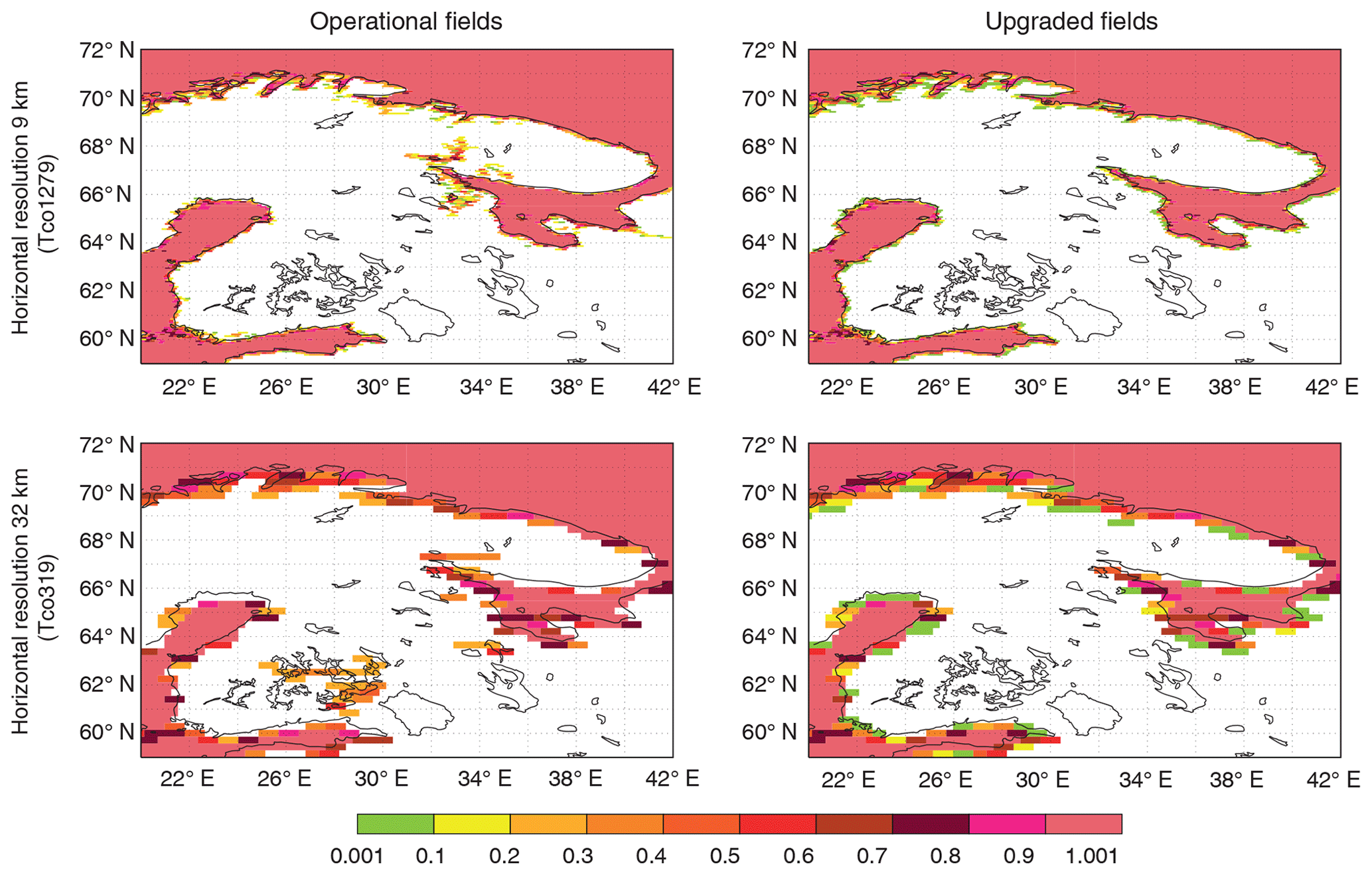
Figure 1Combination of operational and upgraded Frland and Frlake fields showing the remaining ocean water over Finland and north-western Russia (59–72∘ N, 20–42∘ E) at different horizontal resolutions; colours indicate the ocean fraction in each grid box: white – no ocean; pink – fully covered with ocean.
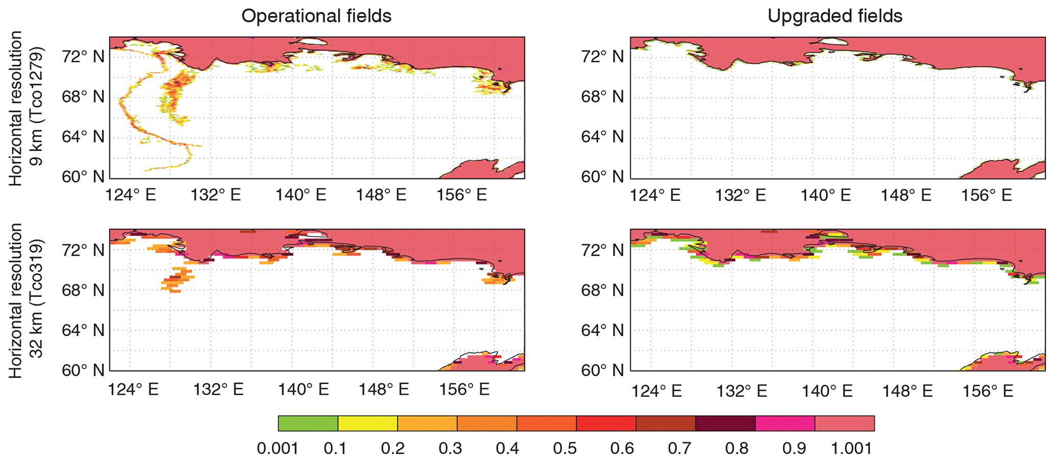
Figure 2Same as Fig. 1 but over north-eastern Russia (60–74∘ N, 122–163∘ E).
The main disadvantage of the current ocean–inland water separating procedure is simplification of a complex coastline (e.g. Finland, Norway) and neglect of small islands. At coarser resolution narrow land parts that separate freshwater lakes and saline ocean disappear (land fraction becomes too small) and coastal lakes and wide estuaries are treated as ocean (the surface temperature is extrapolated from the sea surface temperature of the nearest ocean grid point), which can lead to no-ice conditions during winter at high latitudes or rather low temperatures and almost no diurnal cycle during summer. One example is disappearing islands that separate the freshwater Lake Alexandrina in South Australia from the saline Great Australian Bight (Indian Ocean), which results in flooding of the freshwater lake with the saline ocean and in modelling of perspective to the completely different surface temperature. Figures 1 and 2, left columns, show results of the operational Frland and Frlake field combination (remaining fractional ocean part) at 9 km (Tco1279, upper plots) and 32 km (Tco319, lower plots) horizontal resolutions over the Finland and north-western Russia (59–72∘ N, 20–42∘ E) and north-eastern Russia (60–74∘ N, 122–163∘ E) regions respectively. These plots show how use of the current ocean–inland water separating procedure leads to deep ocean penetration into land and/or separated ocean parts over the land at coarser resolutions. For example, Fig. 1, left column upper plot, at 9 km resolution shows neat separation of inland water and ocean, and Fig. 1, left column lower plot, at 32 km resolution shows that the same water separation procedure leads to deep ocean penetration inland filling Lake Saimaa with salt water through pixels that became not land-dominated at coarser resolution. In addition, several inaccuracies were reported in inland water distribution, such as a too wet Australia and omission of Alqueva Reservoir – the biggest man-made lake in western Europe. All these features required an urgent update.
3.2 Updates
The proposed way of creating lake fields is first to create an LKM compatible with an LWM at a 1 km resolution regular latitude–longitude grid, and then to interpolate both to the needed resolution and grid. This will allow us to preserve water fractions of both types at any resolution independently of Frland. Figures 1 and 2, right columns, give a quick peek at the Frland and Frlake field combination (remaining fractional ocean part) created with the new way at 9 km (Tco1279, upper plots) and 32 km (Tco319, lower plots) horizontal resolutions over the Finland and north-western Russia (59–72∘ N, 20–42∘ E) and north-eastern Russia (60–74∘ N, 122–163∘ E) regions respectively. These plots show how use of the new ocean/inland water separating procedure prevents deep ocean penetration into land and/or separation of ocean parts over the land at coarser resolutions. The proposed methodology is designed bearing in mind quite prompt update of global ecosystem maps: new satellite-based products become freely available with higher and higher resolution more often. To ease the LKM compatibility with LWM upgrade process, the water-type separation procedure is as automated as possible. Dwater is the main parameter to drive lake parameterisation. In the IFS surface scheme FLake runs on each grid point independently of the Frlake, so the Dwater field should be global and as realistic as possible. To achieve this, newer dataset versions, various data source compilations and innovative approaches were used.
The new way of generating the LKM field was (1) to start with a 1 km LWM and (2) to create a consistent 1 km LKM, then (3) to convert a binary LKM field into a fractional Frlake field, and finally (4) to interpolate it to all IFS grids and resolutions. In this case separation between ocean and inland water is done only once at rather high horizontal resolution (∼1 km), which still preserves a lot of coastal features but is computationally (and in a data handling sense) cheaper than the nominal resolution of GlobCover 2009 or GSWE (∼300 m and ∼30 m respectively).
The first step was to aggregate the water cover from the initial GlobCover 2009 10′′ map to 30′′ (43200/21600 grid boxes along longitude and latitude) horizontal resolution. At the end of this step aggregated LWM was also corrected at certain regions where big water distribution errors were reported. The regions and sources are the following.
The Aral Sea is an endorheic lake that used to be one of the four largest lakes in the world. In 1960 its water surface area was 68 900 km2. However, the Aral Sea is shrinking. According to historical records this process started at least in the middle of the 18th century and was accelerated in the 1960s after massive diversion of water for cotton and rice cultivation. GlobCover 2009 shows the Aral Sea for 1998 when its water surface area was 28 990 km2 (less than half of its initial size) (Duhovny et al., 2017); see Fig. 3, upper left plot. Nevertheless, after 1998 shrinking continued. The Aral Sea water surface area started stabilising only in 2014 at an area of 7660 km2 (almost 9 times smaller than its initial size), due to the major Aral Sea recovery programme launched in 2001 by the president of Kazakhstan and supported by the World Bank (The Kazakh Miracle, 2008); see Fig. 3, upper right plot. On the updated map, an up-to-date Aral Sea water distribution from GSWE replaced an outdated one from GlobCover 2009. Only currently present water types were used, i.e. permanent, new permanent and seasonal to permanent.

Figure 3Water distribution from GlobCover 2009 and the GSWE Water Transitions map (only (1) permanent, (2) new permanent and (7) seasonal to permanent water classes are used); yellow colour indicates land, and dark blue indicates water.
The Alqueva Reservoir is the largest man-made water body in western Europe, and it is completely omitted on GlobCover 2009; see Fig. 3, lower left plot. Its surface area is ∼210 km2, with minor interannual/annual variability (Miguel Potes and Rui Salgado, personal communication, 2017). An up-to-date Alqueva Reservoir water distribution from GSWE based on permanent, new permanent and seasonal to permanent water types replaced one from GlobCover 2009; see Fig. 3, lower right plot.
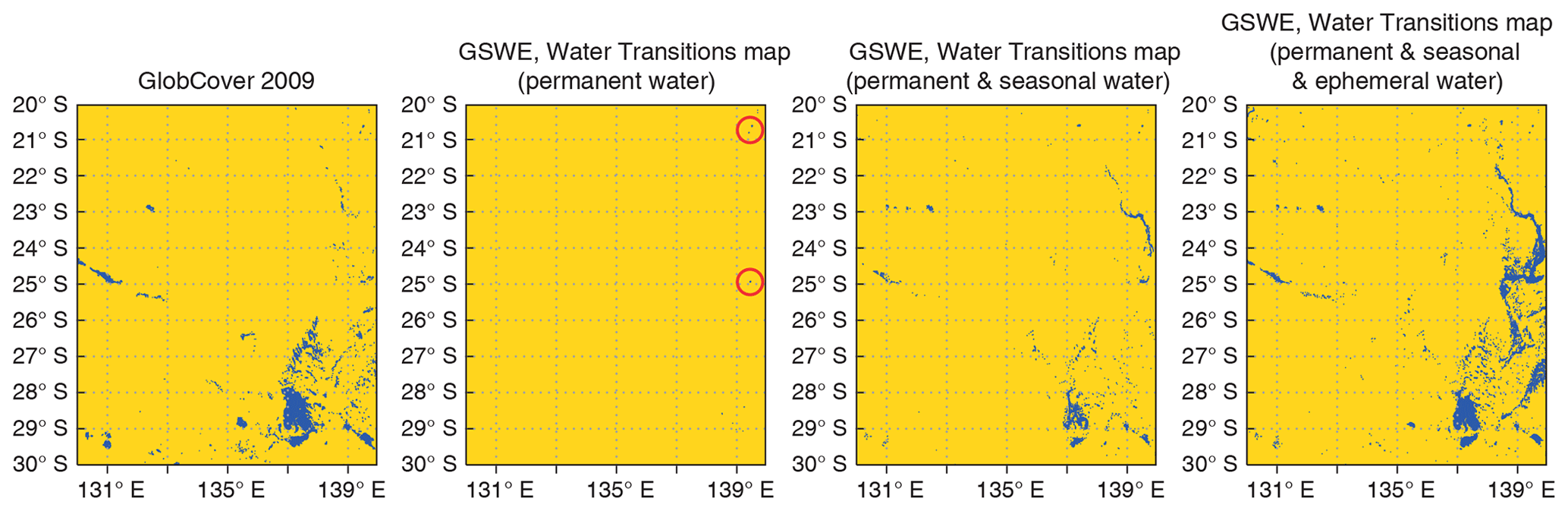
Figure 4Water distribution for the Australian (20–30∘ S, 130–140∘ E) region using GlobCover 2009 and the GSWE Water Transition map with different water class combinations; permanent water stands for a combination of the (1) permanent, (2) new permanent and (7) seasonal to permanent water classes; seasonal water – (4) seasonal, (5) new seasonal and (8) permanent to seasonal; ephemeral water – (9) ephemeral permanent and (10) ephemeral seasonal; yellow colour indicates land, dark blue indicates water, and red circles indicate the locations of Lake Moondarra (upper circle) and Lake Machattie (lower circle).
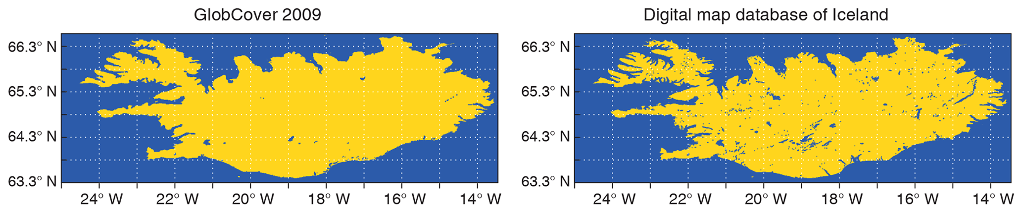
Figure 5Water distribution for Iceland using GlobCover 2009 and the Digital map database of Iceland; yellow colour indicates land, and dark blue indicates water.

Figure 6Phases of LWM water separation for Finland and the north-western part of Russia (a, d, g), the St Lawrence River region (b, e, h), and the Amazon River region (c, f, i): no water separation (a–c), separation with the flood-filling algorithm only (“basic” flooding, d–f) and separation with flood-filling and newly developed pixel-by-pixel water separation algorithms (“extra” flooding, g–i); yellow colour indicates land, dark blue indicates inland water (in d–f and g–i) or total water (in a–c), and light blue indicates ocean.
Australia is the sixth largest (by total area) country in the world, with a vast number of lakes. Lakes are predominantly dry and salty, located in the flat desert regions. Excess inland water on the GlobCover 2009 map was reported for the south-eastern part of Western Australia and the northern part of South Australia (20–30∘ S, 130–140∘ E), as illustrated by Fig. 4. The left plot shows the region in question on GlobCover 2009, with the shallow endorheic Kati Thanda–Lake Eyre (28.37∘ S, 137.37∘ E) in its lower right corner. This lake fills on rare occasions, only a few times a century. Here it is seen in its maximum extent. The right three plots show the same region on the GSWE Water Transitions map with different water class combinations. The combination of permanent, new permanent and seasonal to permanent water classes reflects permanent water; see the second from left plot. This combination has almost no inland water, except the artificial Lake Moondarra (20.59∘ S, 139.54∘ E) and the Lake Machattie area (24.90∘ S, 139.50∘ E), which consists of three lakes: Mipia (usually retains water until the following flood season), Koolivoo (usually dries up by early summer) and Machattie (flooded approximately once in 3 years). Lakes in the Lake Machattie area are fresh when filled by floods but become saline as they dry out. If seasonal, new seasonal and permanent to seasonal water classes (which reflect seasonal water) are added, see the third from left plot, then the region in question has more water, yet much less than on GlobCover 2009. If ephemeral permanent and ephemeral seasonal water classes (which stay for ephemeral water) are also added (see right plot), the region in question gets even more water than on GlobCover 2009, which was reported as being too wet. To make a choice of all year-round plausible water distribution for Australia, experts from Australian National University and the Bureau of Meteorology were consulted. It was explained that there are large-scale ephemeral inundations in inland Australia, but most of them are occasional rather than seasonal (Albert van Dijk, personal communication, 2017). Based on this, it was decided to use the combination of permanent, new permanent and seasonal to permanent water classes from the GSWE Water Transitions map as a whole year static water distribution for Australia; see Fig. 4, second from left plot. This corresponds well to Water Observations from Space for Australia (see https://www.nationalmap.gov.au/#share=s-eUqvVz1ZghXPUBI4ImWweurQppg, last access: 23 September 2019, and http://maps.ga.gov.au/interactive-maps/#/theme/water/map/surfacehydrology, last access: 23 September 2019).
Iceland is located around 63–67∘ N, which makes it quite poor for reliable satellite observations, also due to much cloud and cloud shadow conditions. Figure 5, left plot, shows the GlobCover 2009 water distribution for Iceland. If possible, it is good to complement these data with ground observations (e.g. theodolite, lidar). Here, the Digital map database of Iceland provided by the Icelandic Meteorological Office and referred to as the best available for the regional source of water distribution information (Bolli Palmason and Ragnar Heiðar Þrastarson, personal communication, 2018) was used; see Fig. 5, right plot.
Then corrected LWM produced from GlobCover 2009 (which is available from 85∘ N to 60∘ S) was combined with the RAMP2 dataset over Antarctica and an assumption of no land north of 85∘ N. The resulting field is an updated LWM, further used for upgraded LKM creation.
The next step is the division of LWM water into inland and ocean parts. At the beginning the basic flood-filling algorithm was used. However, with the fine ∼1 km resolution problematic regions with the deep ocean into land penetration (through river estuaries) or merger of different inland water bodies were revealed. Figure 6 shows results of water separation with different techniques at several geographical locations. Upper row plots display no ocean/inland water separation and middle row plots separation with the basic flood-filling algorithm. Left column plots show the region of Finland and the north-western part of Russia, where inland water is neatly separated by the basic flood-filling algorithm. Middle column plots show the region of the St Lawrence River with light ocean penetration into the land through the St Lawrence River and its lakes (i.e. Saint Pierre, Saint Louis and Two Mountains) and the Ottawa River. Right column plots show the region of the Amazon River with deep ocean penetration into the land through the estuary of the Amazon River and nearby lakes (e.g. Grande do Curuai, Itarim), as well as the estuaries of the Xingu River and the Tocantins River with the Tucurui Reservoir. This Amazon River region example also shows several inner water bodies merge, which makes it extremely challenging to automatically map individual lake depth with each water body, as was done in Kourzeneva et al. (2012) for mapping lake depths for GLDB.
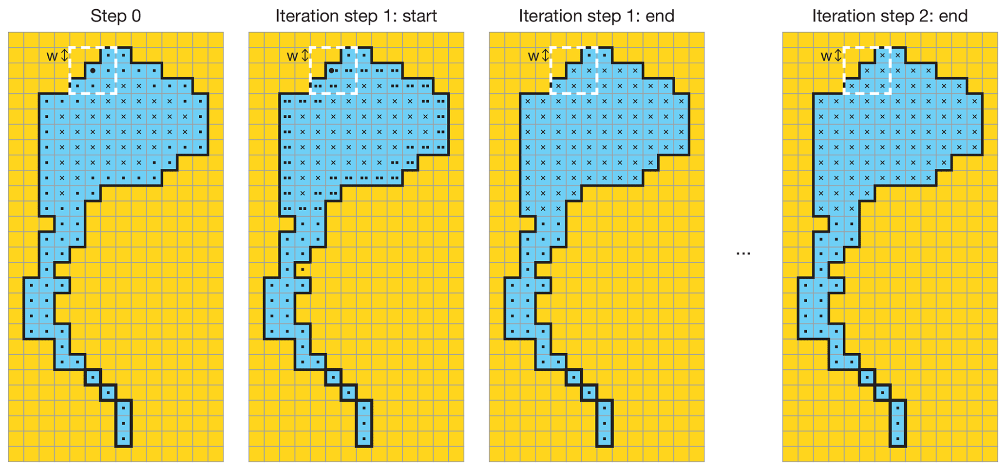
Figure 7Steps of the pixel-by-pixel water separation algorithm. L – number of iterations (here L=2); W – window width (here W=1); ⋅ – water grid box has not only water points in its checking window; x – water grid box has only water points in its checking window; – water grid box has at least one x in its checking window; yellow colour indicates land, and dark blue indicates water.
Table 1List of geographical locations for the water pixel-by-pixel separation algorithm application.

Specially for these complicated situations, when separation should be based on physical and geographical rather than geometrical features, the innovative water body separation algorithm was developed and applied. In general, the algorithm allows us to separate narrow rivers or bays from large water bodies (e.g. lakes or seas). Since it is based on something more than just geometry, it contains two parameters which depend on the resolution and complexity of the regions' coastlines. These parameters should be defined beforehand by relying on expert opinion (i.e. tuning parameters). The algorithm is pixel-by-pixel and iterative. The parameters are
- i.
the window width W – checking radius around the water pixel in question, defined in number of pixels (in Fig. 7 example W=1); and
- ii.
the number of iterations L – how many times the algorithm must be applied over each water body (in Fig. 7 example L=2).
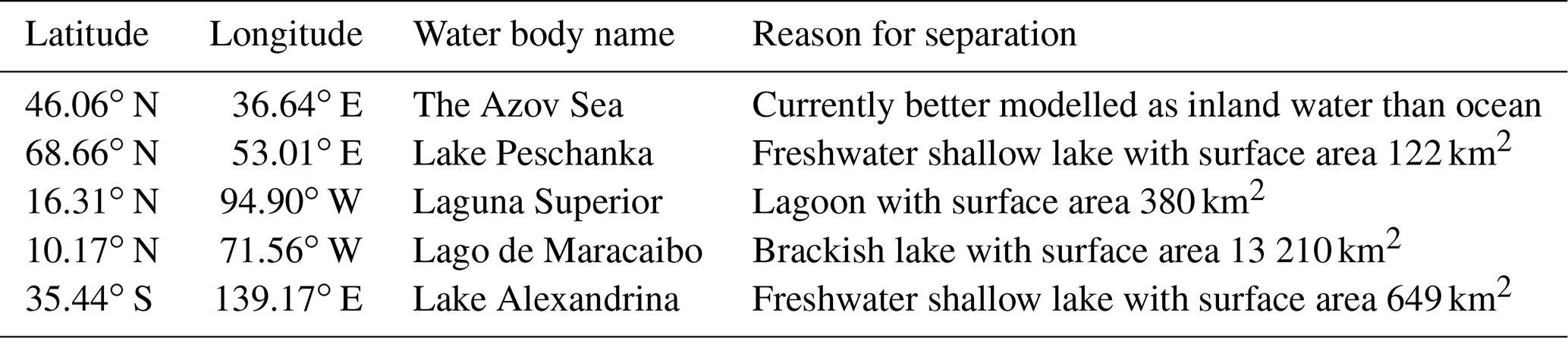
Table 2List of the exceptional water bodies for manual separation from the ocean.
Step 0 of the new algorithm starts by working from the results of the basic flood-filling algorithm. In this case the basic flood-filling algorithm should be applied so that it creates an individual water body mask, to avoid any mismatch between closely located water bodies. Then the new algorithm may be applied to each water body successively. Step 0 is shown in Fig. 7, left plot. At Step 0, each water pixel is marked with “x” if all pixels within the moving window of the W width are water, or “⋅” if at least one pixel in this window is non-water. Next starts the iteration phase that will be repeated L times. At the beginning of each iteration pixels with “⋅” are checked again with the moving window of the W width – if around the pixel in question there is at least one “x” pixel, it is marked as “”; see Fig. 7, second from left plot. At the end of each iteration all “” pixels are changed into “x” and the next iteration starts if required; see Fig. 7, third from left plot. At the end of the iteration phase the considered water body will be divided into several ones; see Fig. 7, right plot – “x” pixels will mark the main part of the water body and “⋅” pixels will mark the narrow rivers or bays. We applied this algorithm to separate automatically large rivers from the ocean – to stop deep penetration of the salt ocean into the land. The W and L parameters are regionally and grid dependent. If they are unsuccessfully defined or the coastal line is too complicated, the negative side-effect of the algorithm will appear – erroneous separation of fjords and bays from the ocean (e.g. in Norway, northern Canada, Greece and on the western coast of the USA). To stay on the safe side all the separated water bodies with the area less than 500 km2 were converted back to ocean. To minimise the tuning process, the new algorithm was applied only for the specific geographical locations, where big river estuaries and lagoon-type freshwater lakes are situated; see Table 1. For the upgrade L=2 and W=3 were used. Figure 6, lower row plots, show results of basic flood-filling and newly developed pixel-by-pixel water separation algorithms use. The left plot in this row shows the region of Finland and the north-western part of Russia, which looks the same as with use of the basic flood-filling algorithm only, because this region has no big river estuaries. The middle plot in the lower row shows the region of the St Lawrence River with neat separation of the freshwater river and saline ocean next to Orleans Island in Quebec (Île d'Orléan). The right plot in the lower row shows the region of the Amazon River with the realistic separation of the ocean and river estuary.
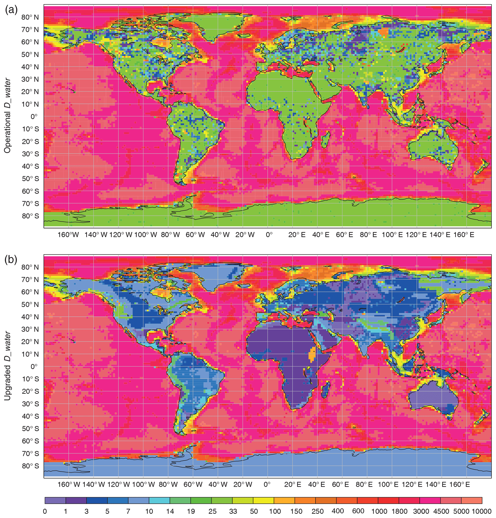
Figure 8Operational (a) and new (b) depth fields at 9 km horizontal resolution (Tco1279); depth values in metres.
The final step in the LWM water separation is the visual check of the significant freshwater coastal lagoons and lakes over the globe, in case some separating islands or spits are missing on the initial ecosystem map. Also, some water bodies such as the Azov Sea and the Caspian Sea are better represented as inland water than ocean due to the current features of the IFS. This leads to a list of exceptional water bodies (see Table 2), which were manually separated from the ocean (the Caspian Sea is marked as a lake automatically), and creation of an updated LKM.
The upgrade of the Dwater field concluded in combination of all the most up-to-date reliable high-resolution global datasets, which are GLDBv3, ETOPO1 and GEBCO. Information from GLDBv3 is used for the mean depth of the inland water bodies, bathymetry of 36 large lakes and the majority of Finnish lakes, ETOPO1 is used for the Great Lakes, and GEBCO is used for the Azov Sea, the Caspian Sea and the ocean bathymetry. The “default” 25 m depth was substituted with depth estimates based on a geological approach (Choulga et al., 2014), which was implemented all around the globe. In rare cases where the geological approach had no value, the “default” depth of 10 m was used. Figure 8 shows the Dwater field at 9 km horizontal resolution (Tco1279): the upper plot is the operational version, the lower plot the new version. On average, all depths became shallower as the “default” depth of 25 m in the operational version was substituted with more realistic values.
The depth aggregation algorithm was also upgraded (from operational simple averaging). The lake depth is not a continuous field, like the air pressure or temperature, and averaging is not the most accurate way of treating it. The new lake depth aggregation is based on the mode (most common) value and the water type (ocean or inland water). Also, now the depth data source is considered if there are in situ measurements, indirect estimates or a “default” value. For the depth aggregation only LWM water pixels are used; ocean and inland water pixels are aggregated separately. In the coastal regions, where both water types are present, Dwater is averaged proportionally to the number of each water type pixel. Ocean pixels are aggregated by averaging as the ocean bathymetry can be considered a continuous field (values change smoothly from point to point). For aggregation of the inland water body depths, the mode is used. The mode is calculated for each type of depth datum separately and the non-zero value with the highest priority is used as an aggregated grid-box depth; the highest priority is given to the value calculated only from the in situ measurement, the second to the value calculated only from the depth indirect estimates, and the lowest to the “default” 10 m depth. This helps to preserve the measured values at rather high resolutions where the lake effect is most pronounced.
Upgraded lake-related fields must be tested prior to operational implementation, as inland water bodies can have significant impact on local climate and weather in terms of 2 m temperature: over 1 K (Balsamo et al., 2012) and up to 10 K (Eerola et at., 2014) respectively. FLake prognostic variables are the mixed-layer temperature TML, the mixed-layer depth, the bottom temperature, the mean temperature of the total water column, the shape factor, the temperature at the ice upper surface, and the ice thickness (IFS Documentation, 2017). Verification is performed in terms of TML and the ice formation/disappearance dates. Modelling results are verified against in situ measurements of lake water surface temperature and ice formation/disappearance dates recorded by the Data and Information Centre of the Finnish Environment Institute (SYKE).
4.1 Model experiment set-up and verification methods
Numerical experiments with the IFS model using operational and upgraded LKM and Dwater were run for 5 years from 1 January 2010 to 31 December 2014, with 3 months of model spin-up from 1 October 2009 to 31 December 2009. Experiments started in the middle of autumn 2009, when all Finnish lakes are mixed till the bottom, to shorten the model spin-up time and to get reliable results straight after ice melting in spring 2010. Experiments run with the IFS CY43R3 model on the triangular cubic octahedral grid with the high horizontal resolution ∼9 km (i.e. Tco1279), in the surface offline mode (i.e. no feedback of the surface to the atmosphere). For the forcing, the lowest model-level variables were taken from the newly available ERA5 reanalysis (C3S, 2017). In ERA5, the lake parameterisation is included in the model. The experiments GTZPOPR (red in all figures) and GTZLNEW (blue in all figures) used operational and upgraded Frlake and Dwater values respectively.
For verification, we used the standard scores: mean error or bias (difference between observed and simulated values), mean absolute error (MAE), and error standard deviation (SD). The statistical significance of the difference in model errors between two experiments was checked with a non-parametric Kruskal–Wallis test (Glantz, 2012) as previously it had been noted that errors have a non-Gaussian distribution. For the Kruskal–Wallis test, data from all compared groups are combined, sorted ascending and ranked; equal values are assigned with their mean rank. The Kruskal–Wallis test statistic H is
where K is the number of groups, nk is the sample volume for group k, N is the total volume of all groups combined, , is the average rank of group k, and is the average rank of combined groups . To estimate the statistical significance, H is compared with a critical value χ2 for (K−1) groups with the significance level α (if not stated differently, α=0.05). If H > χ2, then differences between groups are statistically significant.
In situ SYKE data. SYKE is responsible for producing, storing and distributing Finland's national environmental information and spatial data (SYKE, 2017). SYKE operates more than 30 regular lake and river water temperature measurement sites over Finland. In situ lake water surface temperature measurements and on-shore observations of the lake visible area freeze-up/break-up dates collected by SYKE are used for the model verification. The water temperature is measured every morning during the ice-free season at 08:00 local time, close to the shore, at 20 cm below the water surface (Rontu et al., 2012, Kheyrollah Pour et al., 2017). Temperature measurements and ice formation/disappearance dates from 27 lakes for 2010–2014 are used for verification. Locations of the measurement points are shown in Fig. 9.
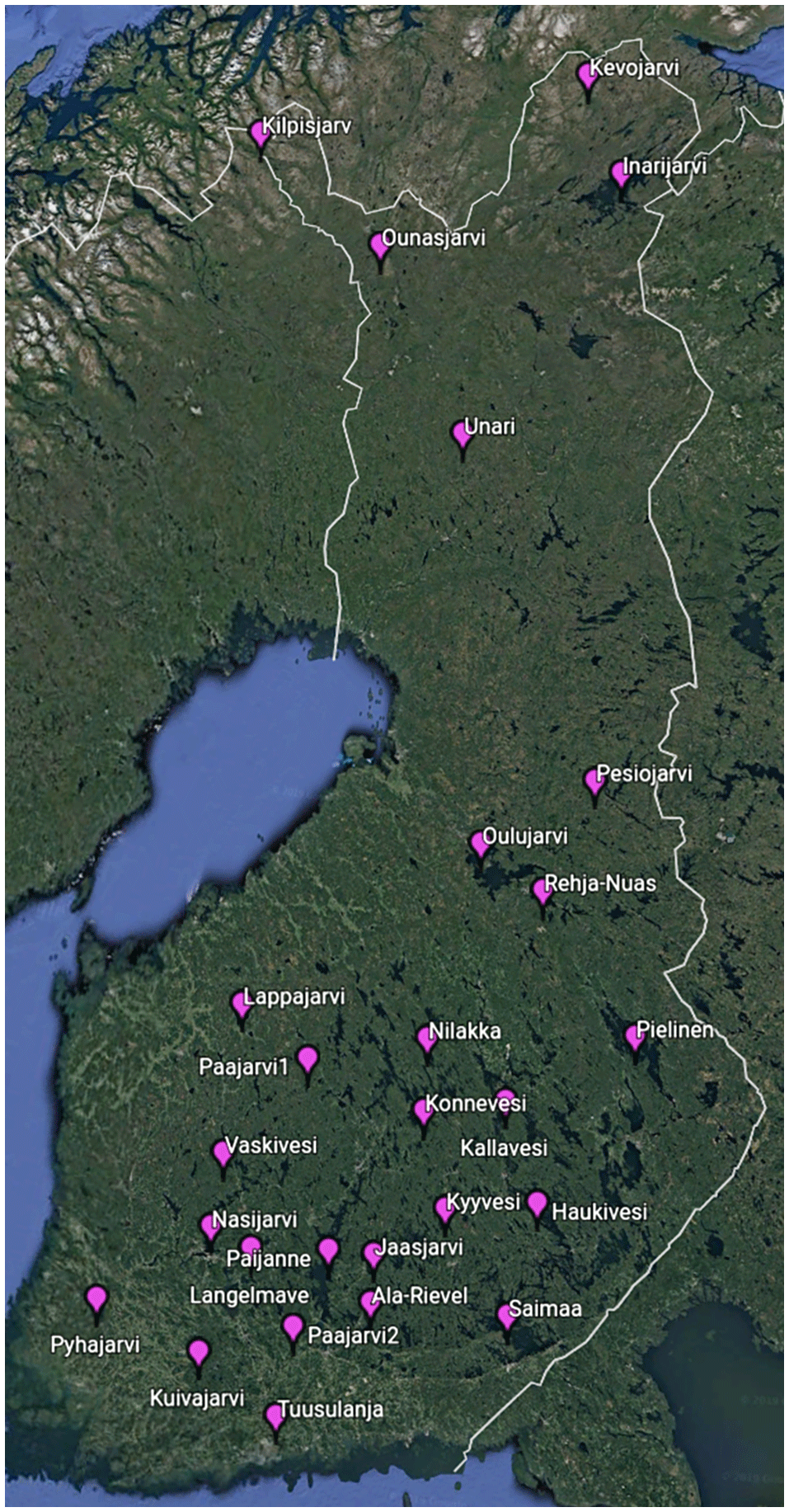
Figure 9Locations of 27 lake verification sites (© Google Maps 2019).
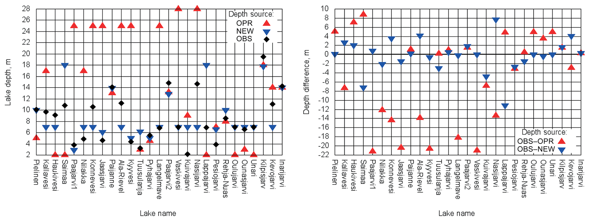
Figure 10Lake depths and their differences in metres for 27 verification sites; OBS – measured by SYKE, OPR – from the ECMWF operational file and NEW – from the upgraded file.
Table 3Locations of 27 verification lake sites; lake morphological parameters measured by SYKE and from ECMWF Tco1279 fields.
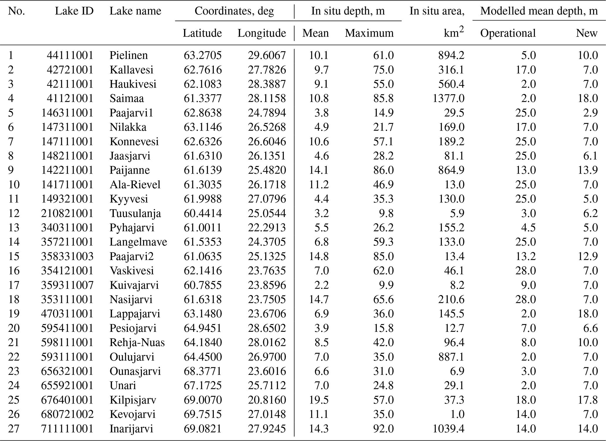
The main morphological properties of lakes are given in Table 3 and Fig. 10. This table also contains Dwater values from the model grid. Differences between in situ depth measurements and Dwater values from the model are due to horizontal resolution: the in situ depth values are from point measurements and the model depth values are from aggregated 9 by 9 km grid boxes. During the Dwater upgrade it was noted that Lake Saimaa has an incorrect mean depth (18.0 m instead of 10.8 m); correction is planned during the next upgrade.
Comparison between the operational and upgraded fields, considering the error as a difference between in situ and modelled values, shows that for 27 selected lake sites even with 9 km resolution the upgraded Dwater values have 25.4 times lower bias (−0.2 m instead of −4.8 m), 3.4 times lower MAE (2.4 m instead of 8.2 m) and 2.7 times lower SD (3.6 m instead of 9.7 m). Changes are statistically significant.
4.2 Model verification results
Measured and modelled lake surface temperatures were compared for the full experiment period 2010–2014. The model values were sampled for the ice-free season at 08:00 local time to correspond to the measured values. Figure 11 shows the bias, MAE, SD and total amount of data used for each site. In general, errors became smaller (modelled values are closer to the measured ones) as the lake depth values became more realistic. Averaging over all 27 lakes, the comparison between two experiments shows that for GTZLNEW bias is lower for 12.5 %, MAE for 13.4 %, and SD for 20.3 %. For some lakes water temperature modelling errors remained the same as their depth values are the same or changed insignificantly in two experiments. These lakes are Paijanne, Pyhajarvi, Paajarvi2, Kuivajarvi, Pesiojarvi, Rehja-Nuas, Kilpisjarvi and Inarijarvi. The only statistically significant deterioration in the temperature scores was for Lake Lappajarvi, whose depth is overestimated 2.5 times in the upgraded Dwater (18.0 m instead of 6.9 m) due to the depth mapping algorithm and/or horizontal resolution of the depth field.

Figure 11MAE, bias, SD and amount of data calculated over the total period of 2010–2014 for 27 verification sites; GTZP (red) – experiment with operational Dwater, GTZL (blue) – with upgraded Dwater.
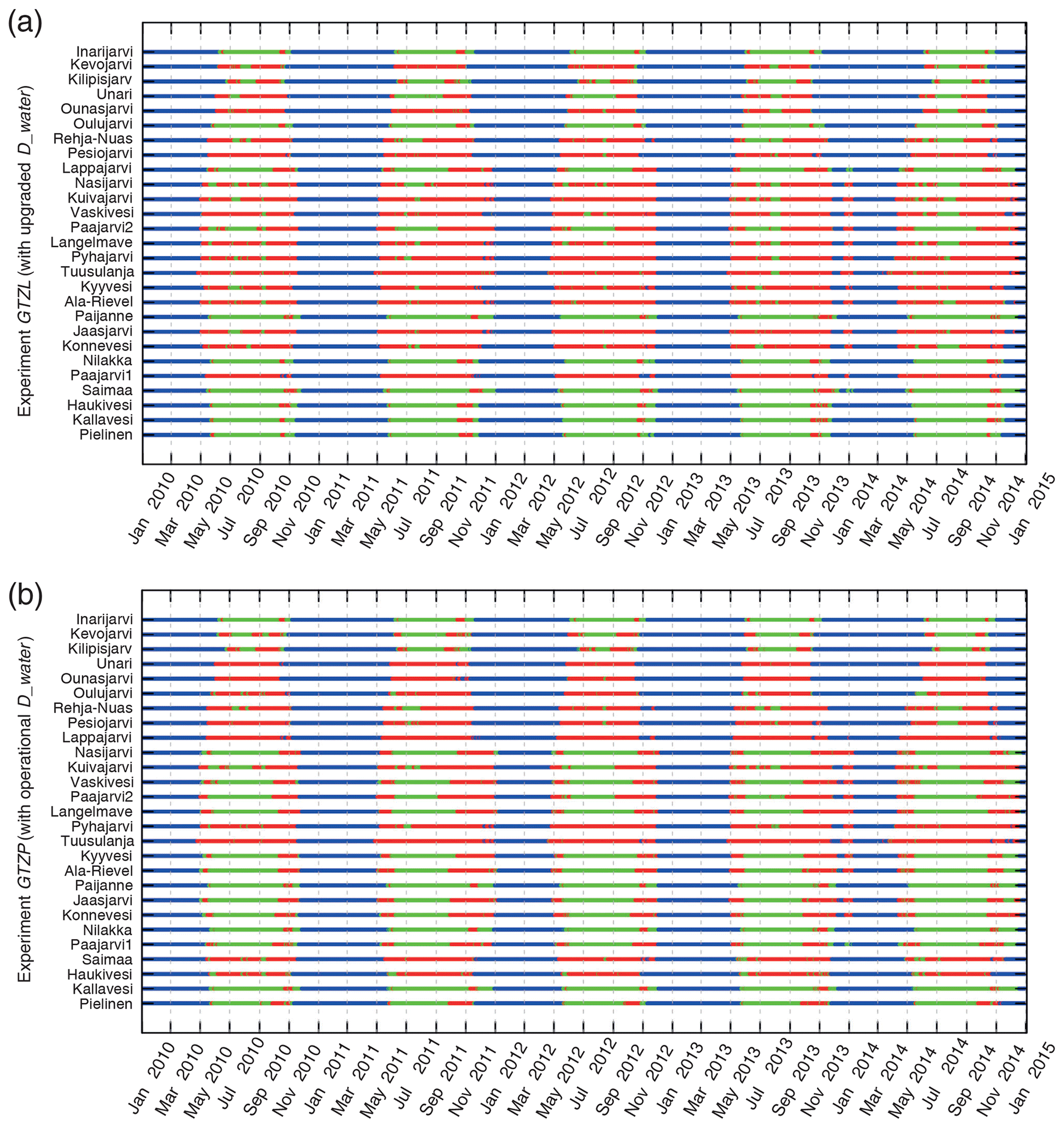
Figure 12Lake seasons for 2010–2014 for 27 verification sites based on operational (b) and upgraded (a) Dwater; blue – lake is ice-covered, red – lake is mixed till the bottom, green – lake is stratified (ice-free and non-mixed, residual period).
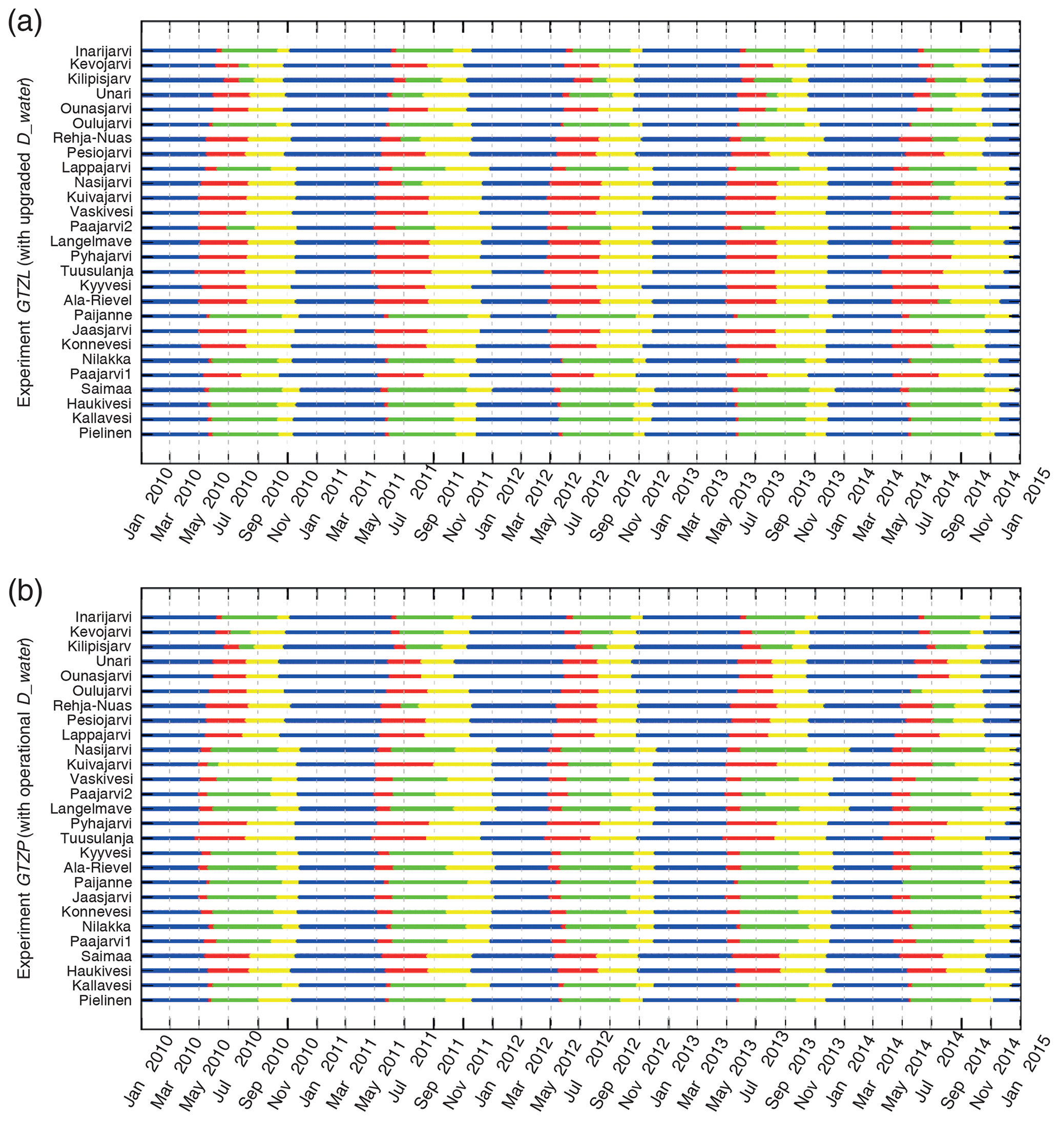
Figure 13Uninterrupted lake seasons for 2010–2014 for 27 verification sites based on operational (b) and upgraded (a) Dwater; blue – winter, red – spring mixing, green – stratified summer, yellow – autumn mixing period.
Model errors may be different during different seasons depending on the model physics. It was shown that FLake has the best performance in the boreal zone during autumn, when lakes are mixed (Choulga and Kourzeneva, 2014), provided that the lake depth is correct. Thus, it is interesting to dig into details and to verify the model results for different seasons, depending on lake mixing regime. Typically, lakes in the boreal zone are dimictic (Lewis, 1983) and have five main seasons in relation to the mixing and ice cover:
- i.
spring mixing, when lakes are mixed till the bottom and the mixed layer depth equals the lake depth,
- ii.
summer, which is the stratified period,
- iii.
autumn mixing period, which is usually longer than the spring one,
- iv.
winter lake cooling period with the inverse temperature stratification, between the temperature of maximal density and start of ice formation, and
- v.
winter, when lakes are covered with ice.
However, this classical pattern is approximate: it may be distorted, depending on the lake depth and the atmospheric forcing. For example, a stratified summer period may be interrupted by a short mixing period. Also, in early spring the inverse temperature stratification may appear. Patterns of mixing and ice periods may be defined from the modelling results. Figure 12 shows ice-covered (blue), mixed (red) and stratified (green) periods, defined for different lakes for the model experiments GTZPOPR and GTZLNEW. Most of the selected lakes show rather complex behaviour with a distorted classical pattern. For example, lakes Paajarvi2 and Kuivajarvi may have multiple ice and mixing periods during the year. Some lakes change patterns from one experiment to another, because of noticeable depth changes (e.g. lakes Haukivesi and Saimaa). To ease the verification process, these patterns were smoothed to better correspond to the dimictic lake classical pattern (simplified by merging the short period of the inverse temperature stratification with autumn mixing). For each lake in both experiments, each year was separated into four main uninterrupted lake seasons, according to the modelling results. Figure 13 shows the results:
- i.
winter period (blue), which contains the merged ice periods when the ice-free time between them is 30 d or less;
- ii.
spring and autumn mixing periods (red and yellow respectively), which contain the merged mixed periods (when the mixed layer depth is approximately equal to the lake depth, with the maximum difference of 10 cm allowed) when the stratified regime between them is 20 d or less; and
- iii.
the stratified summer period (green), which is defined as a residual between spring and autumn periods.
Thus, the spring and autumn mixing periods appeared to be separated by the summer stratified period (e.g. Lake Inarijarvi). With this approximation, some lakes became monomictic (Lewis, 1983), containing no stratified period (e.g. lakes Pyhajarvi and Tuusulanja). For the verification purposes, for these lakes the mixing period was equally divided between spring and autumn seasons.
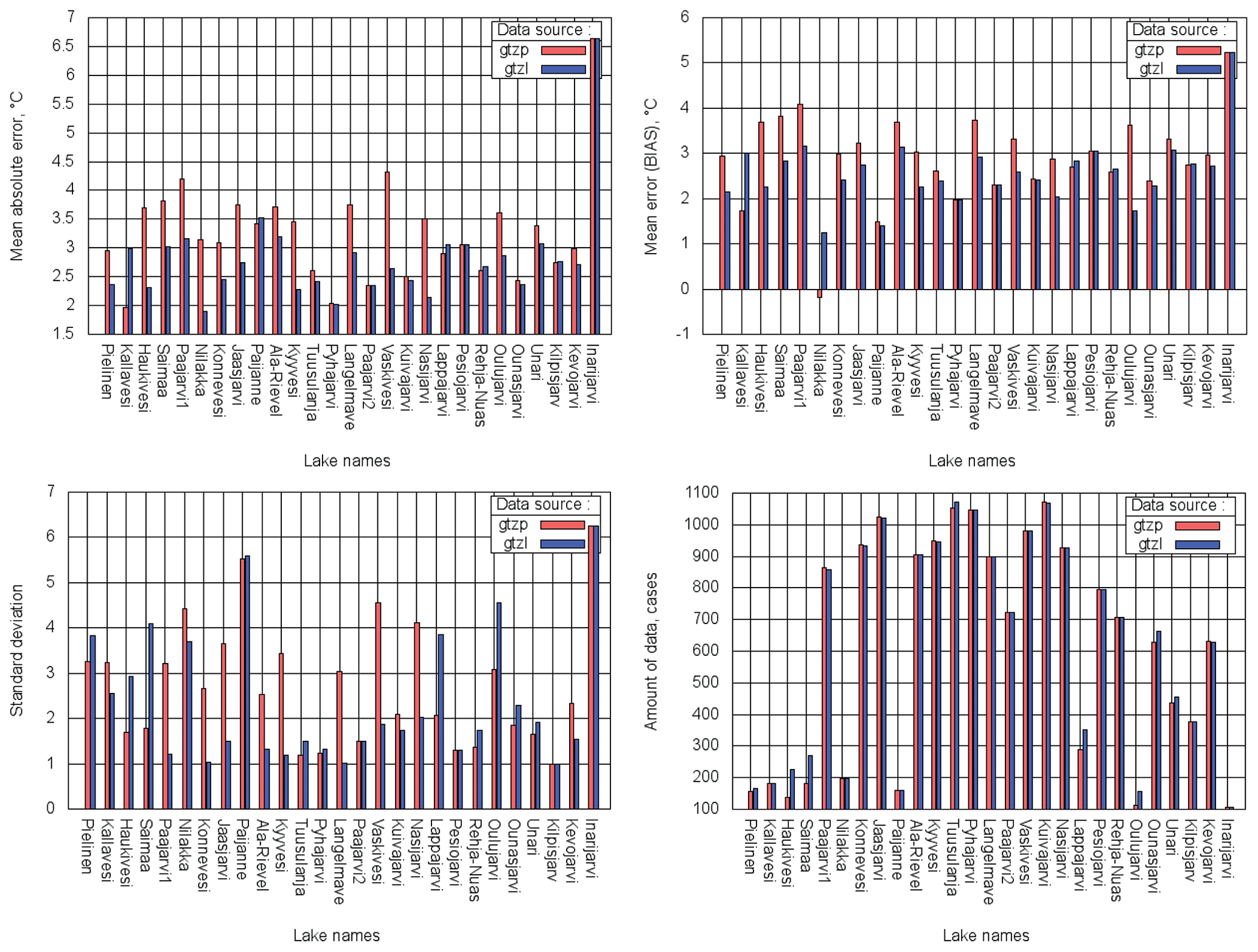
Figure 14MAE, BIAS, SD and amount of data calculated over all mixing periods 2010–2014 for 27 verification sites; GTZP (red) – experiment with operational Dwater; GTZL (blue) – with upgraded Dwater.
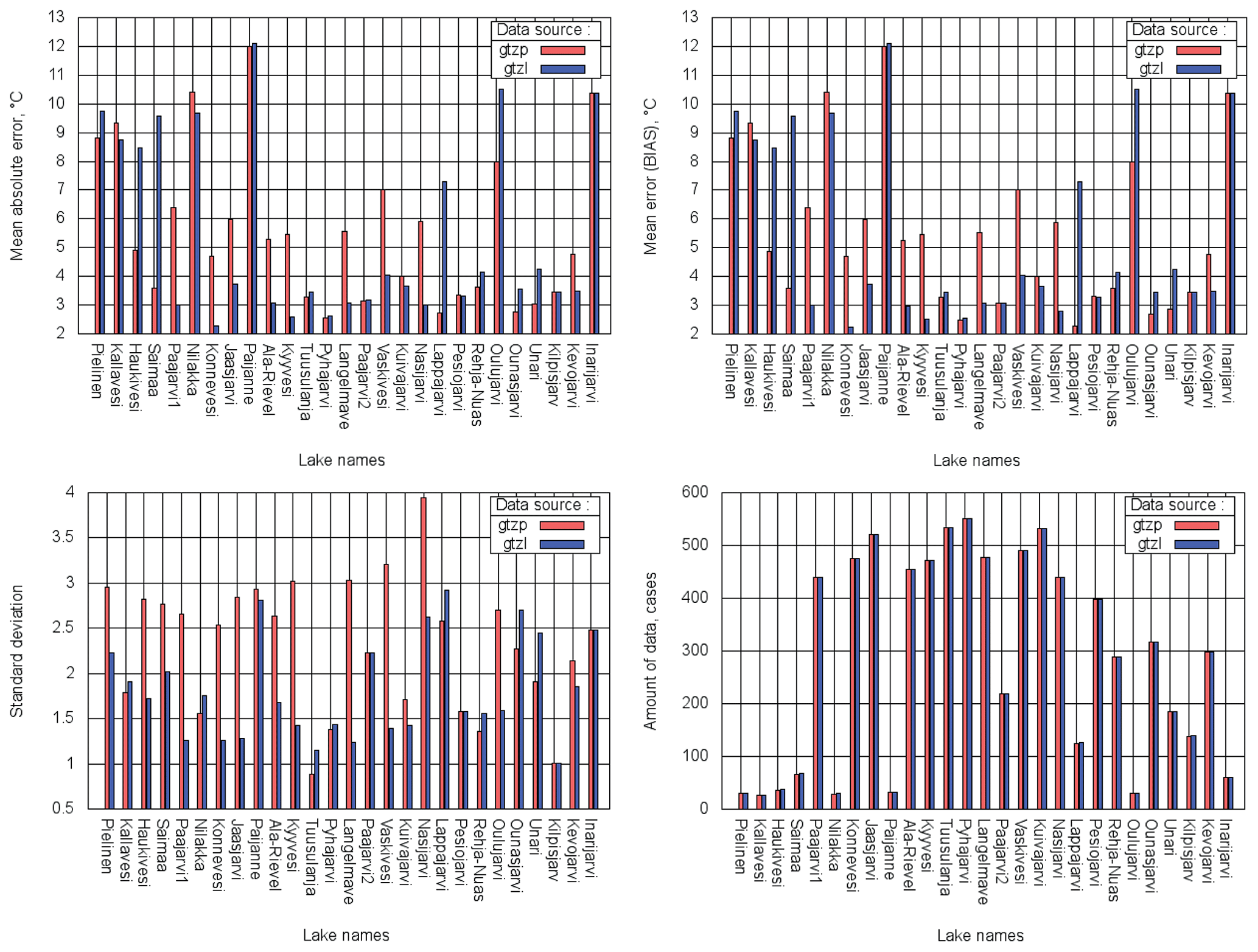
Distribution of model errors in terms of TML depending on a mixing season is shown in Figs. 14–17. The important note is that bias in both experiments in all seasons was predominantly cold (positive) and large. It was so large that SD was smaller than bias. In other FLake model error studies bias was dependent on the season. For example, in Kourzeneva (2014), where forcing was from the High Resolution Limited Area Model (HIRLAM) (Unden et. al, 2002), in summer for the same Finnish lakes there was a strong warm bias, while in spring bias was cold. Errors in TML simulations depend on FLake itself, on the errors in Dwater, which is the main lake model parameter, and on the errors in forcing. Since the results of current experiments differ from the other studies, it should be suggested that in present research errors came from the forcing – ERA5 is supposedly too cold for this region. This problem was previously mentioned in Haiden et al. (2018). Thus, for the Dwater parameter, the situation of compensating errors may appear, depending on a season. Too shallow (underestimated) lake depth can lead to a smaller cold bias during spring mixing and a stronger cold bias during autumn, while the overestimated Dwater parameter can lead to a stronger cold bias in spring and a smaller bias in autumn. In other words, for better spring results it is “advantageous” to underestimate Dwater, but for better autumn results it is “advantageous” to overestimate it. In the stratified summer period, this kind of compensation does not take place, because the mixed layer depth during stable stratification does not depend on the lake depth. However, in summer the TML diurnal cycle depends on Dwater: the deeper the lake, the smaller the TML diurnal cycle amplitude. This may be reflected in SD scores because they relate to the diurnal cycle amplitude in the present experiments. These suggestions are in accordance with the obtained results. For all lakes, where upgraded Dwater was smaller than the operational one, GTZLNEW bias was smaller in spring and larger in autumn compared with GTZPOPR (e.g. lakes Konnevesi and Vaskivesi). And vice versa, for all lakes, where upgraded Dwater was larger than the operational one, GTZLNEW bias was larger in spring and smaller in autumn compared with GTZPOPR (e.g. lakes Haukivesi and Oulujarvi). This was independent of whether new Dwater is closer to the reality or not. For example, for lakes Lappajarvi and Saimaa, where upgraded Dwater became larger and even further from the reality than operational, GTZLNEW autumn bias improved, due to compensating errors (good result for the wrong reason). The only exception was Lake Niilakka, whose autumn bias was negative (warm). For the combined spring–autumn mixing period, bias scores were generally better, or the effect was neutral. For the summer stratified period, the impact of Dwater on the bias scores was neutral or slightly positive. The SD scores were best for the autumn mixing period, when the lake surface temperature diurnal cycle is absent. For lakes Saimaa and Lappajarvi, the summer period SD scores were worse in GTZLNEW compared with GTZPOPR; however, Dwater was worse as well. For the lakes with better Dwater values in GTZLNEW, SD scores improved or remained unchanged for all seasons. The exception was Lake Oulujarvi: its SD scores deteriorated, mainly in autumn.
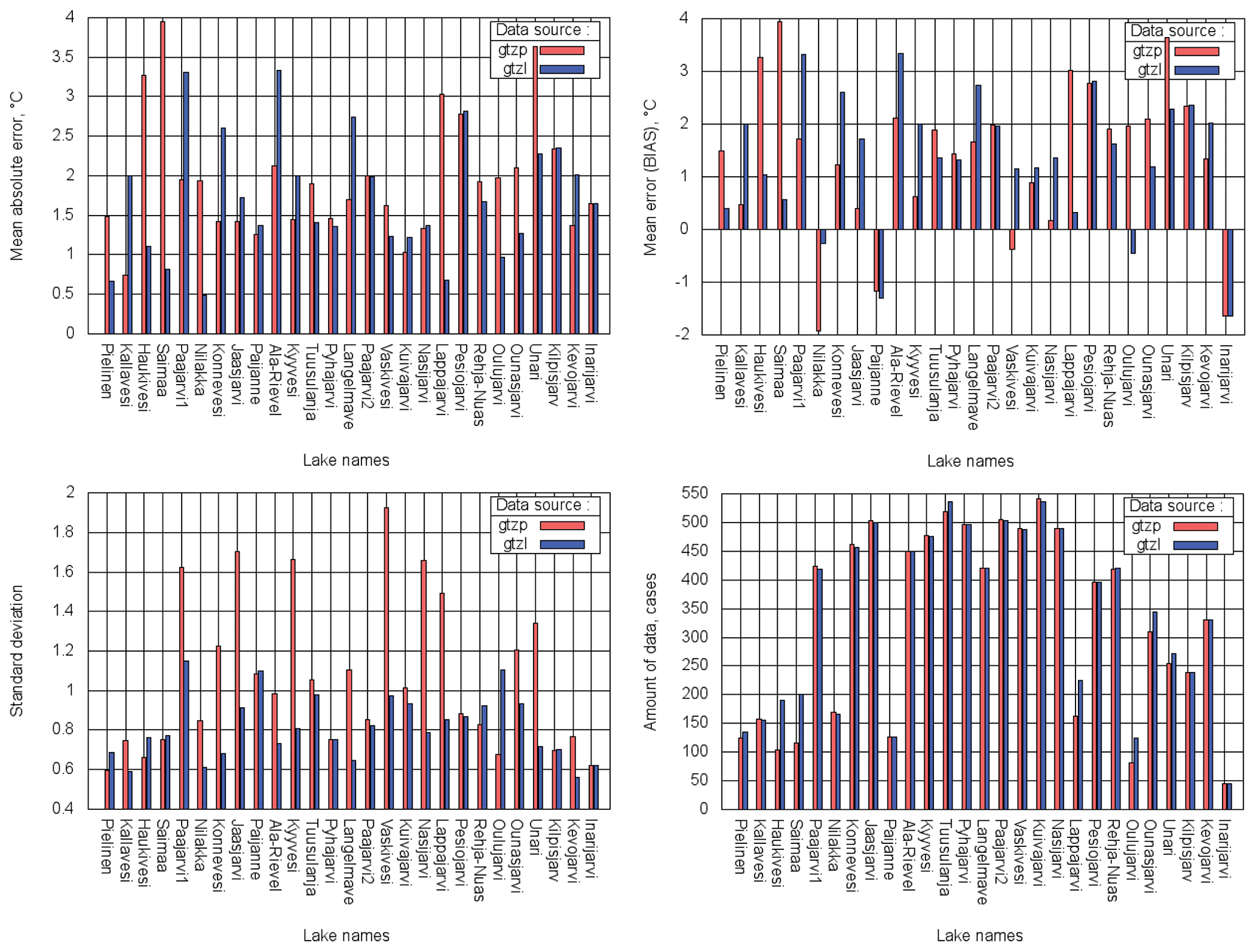
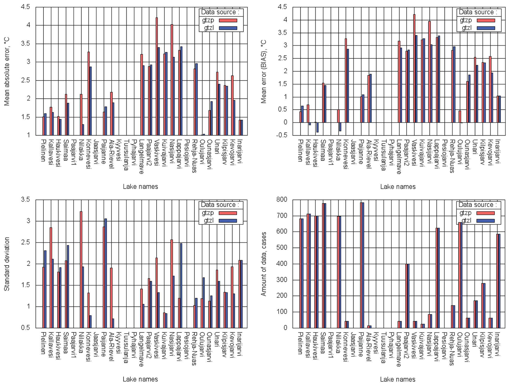
Table 4Ice formation/disappearance dates for 2010–2014 of 27 verification sites; OBS – measured by SYKE; GTZPOPR and GTZLNEW – ECMWF experiments with operational and updated Dwater respectively; improvements in the freeze-up date in GTZLNEW compared with GTZPOPR are marked in bold and degradation in italics (only cases when the difference was larger than 14 d).
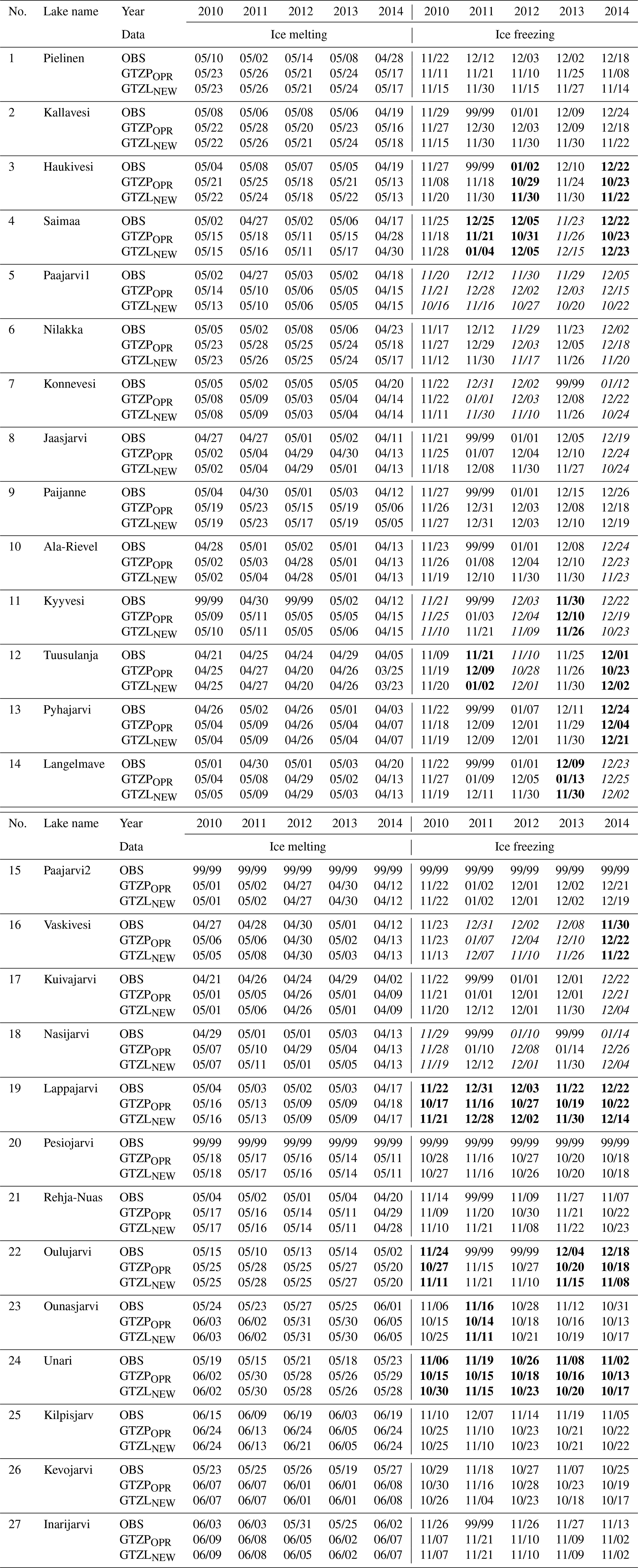
Table 5Locations of in situ water surface temperature and ice formation/disappearance measurement points and distance between them for 27 verification sites; latitude and longitude in degrees, distance in kilometres.
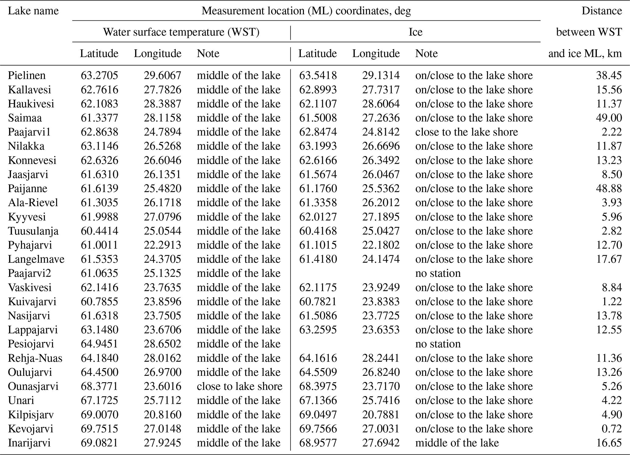
Winter season verification was based on ice formation/disappearance date comparison. Table 4 shows the ice formation/disappearance dates from the SYKE in situ archive and based on experiment results with operational (GTZPOPR) and upgraded (GTZLNEW) Dwater for 27 lake sites. In general, present experiments showed too late ice melt in spring and too early ice formation in autumn; this is in accordance with suggestion of a cold bias in forcing. Thus, compensation may happen also for the errors in freeze-up dates: to compensate for the cold forcing, it is “advantageous” to overestimate the lake depth. Melting dates are mainly dependent on the atmospheric forcing rather than Dwater, but for the freeze-up dates Dwater plays an important role. For the melting dates there was almost no difference between two experiments, but in freeze-up dates the difference was substantial. Errors were large – the ice melt date maximum error was 26 d (lake Niilakka in 2011) and ice freeze-up date maximum error was 61 d (lake Oulujari in 2017, GTZPOPR). The ice-off date errors were not dependent on Dwater; the largest errors corresponded to large-area lakes (e.g. lakes Haukivesi and Kallavesi; see Table 4). It can be explained by the fact that the ice formation/disappearance in situ measurements represent the freeze-up and break-up dates in the visible area around the observer's location (usually on the shore), and due to physiographic features (e.g. complicated rugged coast) and/or meteorological conditions (e.g. low clouds, rain) can be not fully representative for the whole 9 by 9 km grid box. Ice measurement locations differ from temperature measurement locations, and the distance between these two can vary from 0.7 to 49.0 km; see Table 5. SYKE also provides the break-up dates in far central parts of the lake and permanent freeze-up dates of the visible area around the observer's location, but the amount of data is very limited and cannot be used for verification. However, it gives a hint that in the central part of a lake compared with the shore, ice breaks later, up to a week, and close to the coast the permanent ice can appear straight away or even up to a month after the first freeze-up date. The rough estimate of the error due to the model and forcing comes from the break-up date analysis for Lake Kevojarvi. This lake has a small representativeness error, because its surface area is only 1 km2. However, the error in the break-up date for this lake was large – 14 d in both the GTZPOPR and GTZLNEW experiments. Thus, in this verification no difference between experiments GTZPOPR and GTZLNEW was assumed, if it was less than 14 d. In Table 4, improvements in the freeze-up date in GTZLNEW compared with GTZPOPR are marked in bold and degradation in italics, but only for the cases when the difference was larger than 14 d. Otherwise no impact of Dwater is considered. From Table 5, freeze-up dates improved for the lakes with increased Dwater; these lakes became deeper and start to freeze later (e.g. lakes Oulujarvi and Unari). This is independent of whether new Dwater is closer to the reality or not (e.g. for lakes Saimaa and Lappajarvi, the freeze-up dates improved for wrong reasons). If during the upgrade Dwater decreased, errors became larger (e.g. lakes Konnevesi and Vaskivesi). This agrees with the autumn TML bias scores: if they improve, the freeze-up dates improve as well.
4.3 Discussion
Upgraded lake-related fields were tested for 5 successive years to capture short climate deviations (one particular year can be slightly warmer or colder than the average one) yet not to deal with major water distribution and/or inland water body depth changes that can occur in a 10-year period and that would have to be taken into account when compared against in situ measurements. Current verification included only 27 lake sites over Finland which are freely available online; it would be useful to compare model results with measurements from the other countries and climate zones as the IFS is a global forecasting system. For that, data from remote sensing could be beneficial, although they contain gaps and cloud contamination problems. Experiments run with model cycle CY43R3. New cloud physics in the model cycle's recent upgrade led to improvements in calculating 2 m temperature and humidity and precipitations (especially near coasts), which can lead to better agreement of the modelled and in situ lake surface temperature and ice formation/disappearance dates respectively. Verification of operational and upgraded Dwater for 27 Finnish lakes resulted in significant reduction of errors, though it is still possible to upgrade Dwater with new measurements and test new aggregating techniques in order to better represent initial high-resolution lake depth fields. Verification in terms of modelled and in situ lake surface temperature for the whole 5-year period showed general error reduction for 12 %–14 %. Seasonal verification also showed an overall error reduction, although the amount of data during the 5-year period was not sufficient to always have statistically significant results. Seasonal verification also revealed the cold bias in the forcing and situation, when changes in the Dwater parameter compensate for this bias. For more detailed ice formation/disappearance date verification and explanation of the results, first and permanent ice formation/disappearance dates in a far central part of the lake (compatible with an IFS model high-resolution 9 km grid) are needed.
Earth system models used for weather and climate monitoring and forecasting applications, including the IFS, need lower boundary conditions (skin temperature, surface fluxes of heat, moisture and momentum) to calculate the evolution of dynamic processes in the atmosphere and to produce a usable weather forecast. To compute them sufficiently accurately, an up-to-date ecosystem map is needed. Nowadays human activities influence Earth's surface and adapt it to societal needs on relatively short timescales, for example to construct new artificial lakes to supply people and/or crops in arid places with water, or to create new islands to build homes. Inland water bodies can influence local climate by over 1 K (Balsamo et al., 2012), and the influence on local weather can be even more pronounced: correct lake surface state (ice/no ice) in winter conditions can lead to up to 10 K difference in 2 m temperature (Eerola et at., 2014). Major changes in water bodies can occur in just a few years, which means that ecosystem-based maps used for numerical weather prediction need to be updated regularly. The most frequent updates of ecosystem maps come from satellite products, which are becoming available at increasingly high resolution. The main obstacle to using these maps in the model without any modification is that they do not distinguish between ocean and inland water. An automatic algorithm to separate ocean and inland water has been presented in this article. This new algorithm may be used by anyone in the environmental modelling community. This algorithm can also be used to distinguish between rivers and lakes, but it will require more testing and tuning of parameters before it can be applied globally. For the IFS, the most reliable data sources are used to ensure the best possible representation of the global inland water distribution. The continuous water depth field was updated with new ocean and lake bathymetries, new versions of the lake database, and indirect depth estimates based on the geological origin of lakes. Verification of the depth field for 27 Finnish lake sites showed significant lake depth error reductions in the GLDBv3 dataset compared to GLDBv1. Verification in terms of the lake water surface temperature showed an overall error reduction of between 12 % and 14 %. Seasonal lake water surface temperature verification, according to lake mixing periods (spring mixing, summer stratification and autumn mixing), showed an overall error reduction, although forcing in the numerical experiments was too cold, and it may be that this error was compensated for by lake depth parameter errors. Winter season verification based on an ice formation/disappearance date comparison was also influenced by the problem of overly cold forcing and compensating errors. A more detailed ice formation/disappearance date verification and further experiments are clearly needed. The first and permanent ice formation/disappearance dates in the far central part of the lake (compatible with an IFS model high-resolution 9 km grid) would be very helpful for verification. Lake depth and lake cover variability over time are recognised as key aspects for future developments. The present study aims to document the methodology and to provide experimental evidence of its benefits, and it will be used to characterise temporal variations (e.g. in annual or monthly updates).
SYKE datasets are freely available online at http://rajapinnat.ymparisto.fi/api/Hydrologiarajapinta/1.0/ (SYKE, 2017; last access: 23 September 2019). ERA5 reanalysis is freely available online at https://cds.climate.copernicus.eu/cdsapp\#!/home (C3S, 2017; last access: 23 September 2019). Source code of lake model FLake is freely available online at http://www.lakemodel.net (Mironov et al., 2010b; last access: 23 September 2019). Raw output of the IFS model at 9 km resolution for 27 verification sites is available from the corresponding author by request.
All the authors participated in the lake field update (methodology, data generation), the IFS model experiment set-up, and analysis of the in situ and model result comparison. Margarita Choulga wrote the manuscript with contributions from all the other authors.
The authors declare that they have no conflict of interest.
This article is part of the special issue “Modelling lakes in the climate system (GMD/HESS inter-journal SI)”. It is a result of the 5th workshop on “Parameterization of Lakes in Numerical Weather Prediction and Climate Modelling”, Berlin, Germany, 16–19 October 2017.
The authors thank Matti Horttanainen (FMI) for providing in situ TML and ice formation/disappearance dates from the SYKE archive; Laura Rontu (FMI) for useful discussions and help with data handling; Emily Gleeson (Met Eireann), Peter Janssen (ECMWF), and Joe McNorton (ECMWF) for editorial help and assistance; Anabel Bowen (ECMWF) for invaluable help with figure design; and anonymous reviewers 1 and 2 for useful comments. Margarita Choulga was funded by the Earth2Observe project which received funding from the European Union's Seventh Programme for research, technological development, and demonstration under grant agreement no. 603608, and by the CO2 Human Emission (CHE) project which received funding from the European Union's Horizon 2020 research and innovation programme under grant agreement no. 776186.
This research has been supported by Earth2Observe (grant no. 603608) and by CHE (grant no. 776186).
This paper was edited by Miguel Potes and reviewed by two anonymous referees.
Amante, C. and Eakins, B. W.: ETOPO1 1 Arc-Minute Global Relief Model: Procedures, Data Sources and Analysis, NOAA Technical Memorandum NESDIS NGDC-24, National Geophysical Data Center, NOAA, 1–19, https://doi.org/10.7289/V5C8276M, 2009.
Arino, O., Ramos Perez, J. J., Kalogirou, V., Bontemps, S., Defourny, P., and Van Bogaert, E.: Global Land Cover Map for 2009 (GlobCover 2009), European Space Agency (ESA) & Universite catholique de Louvain (UCL), PANGAEA, https://doi.org/10.1594/PANGAEA.787668, 2012.
Balsamo, G., Salgado, R., Dutra, E., Boussetta, S., Stockdale, T., and Potes, M.: On the contribution of lakes in predicting near-surface temperature in a global weather forecasting model, Tellus A, 64, 15829, https://doi.org/10.3402/tellusa.v64i0.15829, 2012.
Bartholome, E. and Belward, A. S.: GLC2000: a new approach to global land cover mapping from Earth observation data, Int. J. Remote Sens., 26, 1959–1977, https://doi.org/10.1080/01431160412331291297, 2005.
Bontemps, S., Defourny, P., Van Bogaert, E., Arino, O., Kalogirou, V., and Ramos Perez, J.: GLOBCOVER 2009 Product description and validation report, UCLouvain & ESA Team, ESA DUE GlobCover website, available at: http://due.esrin.esa.int/page_globcover.php (last access: 23 September 2019), 2011.
Borre, L.: 117 Million Lakes found in Latest World Count, National Geographic Blog Changing Planet, available at: https://blog.nationalgeographic.org/2014/09/15/117-million-lakes-found-in-latest-world-count/ (last access: 23 September 2019), 2014.
Champeaux, J.-L., Han, K.-S., Arcos, D., Habets, F., and Masson, V.: Ecoclimap2: A new approach at global and European scale for ecosystems mapping and associated surface parameters database using SPOT/VEGETATION data – First results, Int. Geosci. Remote Se., 3, 2046–2049, https://doi.org/10.1109/IGARSS.2004.1370752, 2004.
Choulga, M. and Kourzeneva, E.: Verification of indirect estimates for the lake depth database for the purpose of numerical weather prediction and climate modelling, Proceedings of the Russian State Hydrometeorological University: A theoretical research journal, 37, 120–142, 2014.
Choulga, M., Kourzeneva, E., Zakharova, E., and Doganovsky, A.: Estimation of the mean depth of boreal lakes for use in numerical weather prediction and climate modelling, Tellus A, 66, 21295, https://doi.org/10.3402/tellusa.v66.21295, 2014.
CLC2006 technical guidelines: European Environment Agency, 1–66, https://doi.org/10.2800/12134, 2007.
C3S (Copernicus Climate Change Service): ERA5: Fifth generation of ECMWF atmospheric reanalyses of the global climate, Copernicus Climate Change Service Climate Data Store (CDS), available at: https://cds.climate.copernicus.eu/cdsapp#!/home (last access: 23 September 2019), 2017.
Dutra, E., Stepanenko, V. M., Balsamo, G., Viterbo, P., Miranda, P. M. A., Mironov, D., and Schär, C.: An offline study of the impact of lakes on the performance of the ECMWF surface scheme, Boreal Env. Res., 15, 100–112, 2010.
Duhovny, V., Avakyan, I., Zholdasova, I., Mirabdullaev, I., Muminov, S., Roshenko, E., Ruziev, I., Ruziev, M., Stulina, G., and Sorokin, A.: Aral Sea and Its Surrounding, UNESCO Office in Uzbekistan and Baktria Press, 1–120, available at: https://unesdoc.unesco.org/ark:/48223/pf0000260741 (last access: 23 September 2019), 2017.
Eerola, K., Rontu, L., Kourzeneva, E., and Shcherbak, E.: A study on effects of lake temperature and ice cover in HIRLAM, Boreal Env. Res., 15, 130–142, 2010.
Eerola, K., Rontu, L., Kourzeneva, E., Kheyrollah Pour, H., and Duguay, C.: Impact of partly ice-free Lake Ladoga on temperature and cloudiness in an anticyclonic winter situation – a case study using a limited area model, Tellus A, 66, 23929, https://doi.org/10.3402/tellusa.v66.23929, 2014.
Glantz, S. A.: Primer of Biostatistics, Seventh Edition, McGraw-Hill Education, 1–320, available at: https://books.google.co.uk/books?id=EuBdBAAAQBAJ (last access: 23 September 2019), 2012.
Haiden, T., Sandu, I., Balsamo, G., Arduini, G., and Beljaars, A.: Addressing biases in near-surface forecasts, ECMWF Newsletter, 157, 20–25, https://doi.org/10.21957/eng71d53th, 2018.
Hjelmfelt, M. R.: Numerical study of the influence of environmental conditions on lake-effect snowstorms over Lake Michigan, Mon. Weather Rev., 118, 138–150, 1990.
IFS Documentation: CY43R3 – Part IV: Physical processes, ECMWF, 4, available at: https://www.ecmwf.int/node/17736 (last access: 23 September 2019), 2017.
Kheyrollah Pour, H., Choulga, M., Eerola, K., Kourzeneva, E., Rontu, L., Pan, F., and Duguay, C. R.: Towards improved objective analysis of lake surface water temperature in a NWP model: preliminary assessment of statistical properties, Tellus A, 69, 1313025, https://doi.org/10.1080/16000870.2017.1313025, 2017.
Kourzeneva, E.: External data for lake parameterization in Numerical Weather Prediction and climate modelling, Boreal Env. Res., 15, 165–177, 2010.
Kourzeneva, E.: Assimilation of lake water surface temperature observations using an extended Kalman filter, Tellus A, 66, 21510, https://doi.org/10.3402/tellusa.v66.21510, 2014.
Kourzeneva, E., Asensio, H., Martin, E., and Faroux, S.: Global gridded dataset of lake coverage and lake depth for use in numerical weather prediction and climate modelling, Tellus A, 64, 15640, https://doi.org/10.3402/tellusa.v64i0.15640, 2012.
Lewis Jr., W. M.: A Revised Classification of Lakes Based on Mixing, Can. J. Fish. Aquat. Sci., 40, 1779–1787, https://doi.org/10.1139/f83-207, 1983.
Liu, H., Jezek, K. C., Li, B., and Zhao, Z.: Radarsat Antarctic Mapping Project Digital Elevation Model, Version 2, 1 km subset, Boulder, Colorado USA, NASA National Snow and Ice Data Center Distributed Active Archive Center, https://doi.org/10.5067/8JKNEW6BFRVD, 2015.
Manrique-Suñén, A., Nordbo, A., Balsamo, G., Beljaars, A., and Mammarella, I.: Representing Land Surface Heterogeneity: Offline Analysis of the Tiling Method, J. Hydrometeorol., 14, 850–867, https://doi.org/10.1175/JHM-D-12-0108.1, 2013.
Mironov, D.: Parameterization of lakes in numerical weather prediction. Description of a lake model, COSMO Technical Report, 11, 1–41, 2008.
Mironov, D. V., Terzhevik, A., Beyrich, F., Golosov, S., Haise, E., Kirillin, G., Kourzeneva, E., Ritter, B., and Schneider, N.: Parameterization of lakes in numerical weather prediction: description of a lake model, single-column tests, and implementation into the limited-area NWP model, Bound.-Lay. Meteorol., Spec. issue, 1–56, 2006.
Mironov, D., Rontu, L., Kourzenev, E., and Terzhevik, A.: Towards improved representation of lakes in numerical weather prediction and climate models: Introduction to the special issue of Boreal Environment Research, Boreal Environ. Res., 15, 97–99, 2010a.
Mironov, D., Heise, E., Kourzeneva, E., Ritter, B., Schneider, N., and Terzhevik, A.: Implementation of the lake parameterisation scheme FLake into the numerical weather prediction model COSMO, Boreal Env. Res., 15, 218–230, 2010b.
Mironov, D., Ritter, B., Schulz, J.-P., Buchhold, M., Lange, M., and Machulskaya, E.: Parameterization of sea and lake ice in numerical weather prediction models of the German Weather Service, Tellus A, 64, 17330, https://doi.org/10.3402/tellusa.v64i0.17330, 2012.
Notaro, M., Holman, K., Zarrin, A., Fluck, E., Vavrus, S., and Bennington, V.: Influence of the Laurentian Great Lakes on Regional Climate, J. Climate, 26, 789–804, 2013.
Pekel, J.-F., Cottam, A., Gorelick, N., and Belward, A. S.: High-resolution mapping of global surface water and its long-term changes, Nature, 540, 418–422, https://doi.org/10.1038/nature20584, 2016.
Quaife, T. and Cripps, E.: Bayesian Analysis of Uncertainty in the GlobCover 2009 Land Cover Product at Climate Model Grid Scale, Remote Sens., 8, 314, https://doi.org/10.3390/rs8040314, 2016.
Rontu, L., Eerola, K., Kourzeneva, E., and Vehvilainen, B.: Data assimilation and parametrisation of lakes in HIRLAM, Tellus A, 64, 17611, https://doi.org/10.3402/tellusa.v64i0.17611, 2012.
Samuelsson, P., Kourzeneva, E., and Mironov, D.: The impact of lakes on the European climate as simulated by a regional climate model, Boreal Environ. Res., 15, 113–129, 2010.
Stepanenko, V., Machulskaya, E., Glagolev, M., and Lykossov, V.: Numerical Modeling of Methane Emissions from Lakes in the Permafrost Zone, Izv. Atmos. Ocean. Phy., 47, 252–264, https://doi.org/10.1134/S0001433811020113, 2012.
Stepanenko, V., Mammarella, I., Ojala, A., Miettinen, H., Lykosov, V., and Vesala, T.: LAKE 2.0: a model for temperature, methane, carbon dioxide and oxygen dynamics in lakes, Geosci. Model Dev., 9, 1977–2006, https://doi.org/10.5194/gmd-9-1977-2016, 2016.
SYKE: Data and Information Centre, available at: http://www.syke.fi/en-US/SYKE_Info/Organisation/Data_and_Information_Centre(3037) (last access: 23 September 2019), 2017.
The Kazakh Miracle: Recovery of the North Aral Sea, Environment News Service (ENS), available at: http://www.ens-newswire.com/ens/aug2008/2008-08-01-01.asp (last access: 23 September 2019), 2008.
Thiery, W., Davin, E. L., Panitz, H.-J., Demuzere, M., Lhermitte, S., and Lipzig, N.: The Impact of the African Great Lakes on the Regional Climate, J. Climate, 28, 4061–4085, https://doi.org/10.1175/JCLI-D-14-00565.1, 2015.
Thiery, W., Gudmundsson, L., Bedka, K., Semazzi, F. H. M., Lhermitte, S., Willems, P., Van Lipzig, N. P. M., and Seneviratne, S. I.: Early warnings of hazardous thunderstorms over Lake Victoria, Environ. Res. Lett., 12, 7, https://doi.org/10.1088/1748-9326/aa7521, 2017.
Tranvik, L. J., Downing, J., Cotner, J., Loiselle, S., Striegl, R., Ballatore, T. J., Dillon, P., Finlay, K., Fortino, K., Knoll, L. B., Kortelainen, P. L., Kutser, T., Larsen, S., Laurion, I., Leech, D., Mccallister, S., Mcknight, D., Melack, J. M., Overholt, E., and Weyhenmeyer, G. A.: Lakes and reservoirs as regulators of carbon cycling and climate, Limnol. Oceanogr., 54, 2298–2314, https://doi.org/10.4319/lo.2009.54.6_part_2.2298, 2009.
Unden, P., Rontu, L., Jarvinen, H., Lynch, P., Calvo Sánchez, F. J., Cats, G., Cuxart, J., Eerola, K., Fortelius, C., García-Moya, J. A., Jones, C., Lenderink, G., McDonald, A., McGrath, A., Navascués, R. B., Woetman-Nielsen, N., Odegaard, V., Rodríguez Camino, E., Rummukainen, M., Room, R., Sattler, K., Hansen Sass, B., Wichers Schreur, B., Sigg, R., and Tijm, A.: HIRLAM-5 scientific documentation, Swedish Meteorological and Hydrological Institute, available at: https://www.researchgate.net/publication/278962772_HIRLAM-5_scientific_documentation (last access: 23 September 2019), 2002.
Vavrus, S., Notaro, M., and Zarrin, A.: The role of ice cover in heavy lake-effect snowstorms over the Great Lakes Basin as simulated by RegCM4, Mon. Weather Rev., 141, 148–165, 2013.
Verpoorter, C., Kutser, T., Seekell, D. A., and Tranvik, L. J.: A Global Inventory of Lakes Based on High-Resolution Satellite Imagery, Geophys. Res. Lett., 41, 6396–6402, https://doi.org/10.1002/2014GL060641, 2014.
Walter, K. M., Zimov, S. A., Chanton, J. P., Verbyla, D., and Chapin, F. S.: Methane bubbling from Siberian thaw lakes as a positive feedback to climate warming, Nature, 443, 71–75, 2006.
Walter, K. M., Smith, L. C., and Chapin, F. S.: Methane bubbling from northern lakes: present and future contributions to the global methane budget, Philos. T. Roy. Soc. A, 365, 1657–1676, https://doi.org/10.1098/rsta.2007.2036, 2007.
Weatherall, P., Marks, K. M., Jakobsson, M., Schmitt, T., Tani, S., Arndt, J. E., Rovere, M., Chayes, D., Ferrini, V., and Wigley, R.: A new digital bathymetric model of the world's oceans, Earth and Space Science, 2, 331–345, https://doi.org/10.1002/2015EA000107, 2015.