the Creative Commons Attribution 4.0 License.
the Creative Commons Attribution 4.0 License.
 | 24 Sep 2019
Sediment transport modelling in riverine environments: on the importance of grain-size distribution, sediment density, and suspended sediment concentrations at the upstream boundary
Jérémy Lepesqueur
Renaud Hostache
Núria Martínez-Carreras
Emmanuelle Montargès-Pelletier
Christophe Hissler
Hydromorphodynamic models are powerful tools for predicting the potential mobilization and transport of sediment in river ecosystems. Recent studies have shown that they are able to predict suspended sediment matter concentration in small river systems satisfactorily. However, hydro-sedimentary modelling exercises often neglect suspended sediment properties (e.g. sediment densities and grain-size distribution), which are known to directly control sediment dynamics in the water column during flood events. The main objective of this study is to assess whether a better representation of such properties leads to an improved performance in the model. The modelling approach utilizes a fully coupled hydromorphodynamic model based on TELEMAC-3D (v7p1) and an enhanced version of the sediment transport module SISYPHE (based on v7p1), which allows for a refined sediment representation (i.e. 10-class sediment mixtures instead of 2-class mixtures and distributed sediment density instead of uniform). The proposed developments of the SISYPHE model enable us to evaluate and discuss the added value of sediment representation refinement for improving sediment transport and riverbed evolution predictions. To this end, we used several model set-ups to evaluate the influence of sediment grain-size distribution, sediment density, and suspended sediment concentration at the upstream boundary on model predictions. As a test case, we simulated a flood event in a small-scale river, the Orne river in north-eastern France. Depending on the model set-up, the results show substantial discrepancies in terms of simulated bathymetry evolutions. Moreover, the model based on an enhanced configuration of the sediment grain-size distribution (10 classes of particle sizes) and with distinct densities per class outperforms the standard SISYPHE configuration, with only two sediment grain-size classes, in terms of simulated suspended sediment concentration.
- Article
(1093 KB) - Full-text XML
- BibTeX
- EndNote


In the last 2 centuries, many areas have undergone rather fast demographic, industrial and urban development. This intense land occupancy has affected the quality of surface waters, which became the receptacle of anthropogenic effluents from various origins (Whitman, 1998; Heise and Förstner, 2006, 2007; Grabowski et al., 2011). In this context, several rivers in north-eastern France were strongly modified (e.g. rectification of riverbeds and dam building) and received high amounts of domestic and industrial effluents linked to steel-making activities located near water sources (Kanbar et al., 2017). As a consequence of these past effluent emissions, riverbed sediments often remain contaminated, although part of the settled material has been dredged and removed (Kanbar et al., 2017). The remobilization of these riverbed sediments during flood events can subsequently affect water quality and contaminate floodplains (Carter et al., 2006; Hissler and Probst, 2006) and therefore requires thorough investigations (SEDNET, 2003). There is, consequently, a clear need to predict the potential resuspension and transport of sediment in these heavily polluted river systems.
River sediments are heterogeneous aggregates, composite structures composed of amorphous or poorly crystalline mineral particles, organic matter, and biological matter (biofilms, bacteria, viruses, and biomacromolecules). While fresh sediment deposits are often close to fluid mud, older and deeper riverbed sediments tend to be consolidated, with the state of consolidation higher for deeper sediment. These vertical gradients complicate the modelling of sediment erosion, transport, and deposition. Past studies have shown that hydromorphodynamic models are powerful tools for predicting these processes and are able to simulate suspended sediment concentration (SSC) satisfactorily. However, most studies were conducted in coastal, lacustrine, estuarial, and fluvial areas (e.g. Villaret et al., 2013), with far fewer studies done on small river systems (e.g. González-Sanchis et al., 2014; Hostache et al., 2014; Hissler et al., 2015, Barrière et al., 2015). Hydromorphodynamic models often simulate sediment dynamics according to three main processes, namely erosion, transport (via suspended load and bedload), and deposition. Transport equations assume that sediment motion begins when the riverbed shear stress goes beyond a threshold value that depends mainly on the grain diameter and sediment density for non-cohesive sediment. Moreover, sediment density strongly influences sediment settling velocity and advection, which govern erosion and deposition via the sediment mass balance. In this context, Hostache et al. (2014) highlighted that simulated sediment transport, erosion, and deposition are especially sensitive to particle fall velocity, which depends on grain diameter and sediment density. These two parameters therefore control the preferential zones of deposition, since particles with lower or higher fall velocity will settle in different places. Most of the time, hydromorphodynamic models consider sediment to be an ensemble of individual spherical particles. For evident reasons, these models do not simulate sediment particles individually but rather define the so-called sediment grain-size classes and simulate sediment transport separately for each class. Belleudy (2000, 2001) and Guillou et al. (2010) emphasized the paramount importance of using an enhanced sediment grain-size distribution representation to accurately simulate sediment transport in both coastal and river environments. It has also been shown that a uniform grain-size distribution for bedload transport can lead to an overprediction in sediment fluxes by a factor of 5 (Durafour et al., 2015). Durafour et al. (2015) compared various empirical formulations of bedload during tidal cycles and found that distributing bedload fluxes over a larger number of grain-size classes significantly reduced differences between predictions and in situ observations. However, the majority of recent studies still consider only one or two sediment grain-size classes with uniform density (e.g. Qilong and Toorman, 2015; Hostache et al., 2014), and, in many of them, even a unique median grain-size class of sediment is used (García Alba, 2014; Warner et al., 2010). A formal evaluation of model performance when using a larger number of grain-size classes and distributed sediment density is thus still missing.
Here, we further develop an existing hydromorphodynamic model based on the dynamic coupling of TELEMAC-3D and SISYPHE in order to enhance the sediment grain-size and density representations. The objective is therefore to evaluate and discuss the eventual benefits of considering a larger number of grain-size classes and a distributed sediment density for improving sediment transport and riverbed evolution predictions. This paper is divided into four sections. First, we present the hydromorphodynamic model and our developments. Second, we describe the study area, the available observation dataset, and the experimental design. Next, we present and discuss the results. Finally, we summarize our findings and propose perspectives for future developments in hydromorphodynamic modelling.
The proposed modelling framework is based on TELEMAC-MASCARET (Hervouet, 2007). The fluid hydrodynamics are simulated using the TELEMAC-3D model, which solves the Navier–Stokes equations in the hydrostatic mode. Morphodynamic and sediment transport modelling is carried out using the SISYPHE model (Villaret, 2010, 2013), an additional TELEMAC-MASCARET module. We adopted this modelling framework for two main reasons: (i) the two aforementioned models are based on an unstructured mesh of finite elements, which is particularly suitable for modelling river and coastal areas, as it allows the simulation of complex geometries, and (ii) they can be dynamically coupled. The dynamic coupling of the two models is especially relevant for sediment transport and morphodynamic modelling, as it allows, at each simulation time step, the effect of riverbed changes on the flow and vice versa to be taken into account. SISYPHE decomposes the dynamic sediment processes into sediment transport, erosion, and deposition. Sediment transport is decoupled into bedload and suspended load, which allows the computation of sediment concentrations in the water column.
2.1 Friction and bed shear stress
The bed shear stress (τ) is the hydrodynamic variable that controls sediment transport through erosion and deposition (Villaret et al., 2013). TELEMAC-3D uses a roughness coefficient for the bottom energy dissipation by friction. This friction is responsible for the bed shear stress that controls erosion and deposition. In this study, TELEMAC-3D and SISYPHE are coupled dynamically and the friction is calculated based on the Nikuradse law (Nikuradse, 1932). Previous studies on an estuary system (Lepesqueur, 2009) showed the importance of using spatially distributed friction coefficients instead of a single uniform coefficient in order to yield more accurate predictions of current velocities and directions, especially in shallow water where friction is controlled by the apparent roughness of the sediment and the bed forms.
The friction as a function of the bottom-sediment grain size (Lepesqueur, 2009), according to the Nikuradse law, is computed as follows:
In Eq. (1), ρ is the water density, u* the friction velocity, z1 the “altitude of the first horizontal plane above the bottom”, the near-bed-flow velocity, κ=0.4 the von Kármán constant, ks≈2.5d50 the Nikuradse bed roughness, and d50 the median bottom-sediment grain size.
2.2 Bed evolution
When TELEMAC-3D and SISYPHE are coupled dynamically, the latter computes the bed evolution using the Exner equation (Exner, 1920, 1925) and transmits the bed-level state to the former at each time step. The bed evolution is taken into account by the hydrodynamic model to better predict the flow intensity and direction. It is computed based on the divergence of the bedload flux and the net deposition and erosion due to the suspended sediment transport:
In Eq. (2), n is the bed sediment porosity, Zf the bottom elevation, Qb the bedload flux per unit width, and E and D the erosion and deposition rates at elevation z=a, corresponding to the interface between bedload and suspended load.
2.3 Suspended sediment transport
The SSC is computed using the following equation of advection–diffusion:
In Eq. (3), C is the depth-average SSC, γt the diffusion coefficient, U and V the depth-averaged flow velocities in the x and y directions, respectively, and h the water depth.
2.4 Erosion and deposition rates
SISYPHE allows the transport of cohesive and non-cohesive sediment mixtures to be simulated and is able to consider these two types of sediment separately. This is a relevant point, as the processes governing the erosion and deposition of these two types of sediment are markedly different (Villaret et al., 2010). In SISYPHE, the distinction between cohesive (i.e. mud) and non-cohesive sediment is based on the sediment diameter: the sediment is considered cohesive below 63 µm (silts and clays) and non-cohesive beyond 63 µm. For the cohesive sediment, a uniform suspended concentration across the water column is considered, and the Krone (1962) and Partheniades (1965) formulation (see Eqs. 4–5) governs the erosion and deposition rates:
In Eq. (4), M is the Partheniades constant set to kg s−1 m−2, τ0 the shear stress, and τce the critical shear stress. The critical shear stress of the mud was measured in-situ using a scissometer. The critical value was estimated to be 0.48 Pa for the top layer and 0.84 Pa at 15 cm depth. A linear interpolation is used to attribute an individual critical shear stress value to each bottom layer:
In Eq. (5), C is the suspended mud concentration in the water column, τcd the critical constraint of deposition (set at 0.001 Pa), and Ws the fall velocity computed based on sediment diameter according to Zanke's formulation (Zanke, 1977):
In Eq. (6), is the sediment relative density, where ρs is the sediment particle density, ρ the water density, g the gravitational constant, ν the fluid kinematic viscosity, and d the sediment particle diameter.
Depending on the mud fraction (i.e. ratio between mud and total sediment mass) in the top layer of the riverbed sediment, SISYPHE treats non-cohesive sediment erosion according to the so-called non-cohesive and cohesive regimes. The formulation used for the erosion of sediment mixtures follows the developments of Waeles (2005), which are based on the model proposed by Van Ledden (2001) according to the observations made by Mitchener and Torf (1996), Panagiotopoulus (1997), and Mignot (1989). Panagiotopoulus (1997) stated that the critical shear stress of sand depends on the mud fraction: at mud fractions lower than 30 %, the critical shear stress of sand is slightly influenced by the mud content, whereas it reaches that of pure mud for fractions higher than 50 %.
Following these findings, in SISYPHE, the non-cohesive sediment is eroded as pure sand (non-cohesive regime) if the mass fraction of mud is below 30 % and as mud (cohesive regime) if the mass fraction of mud is beyond 50 % in the top layer of the riverbed sediment. Moreover, following Waeles (2005) and Villaret (2010), a linear interpolation between the two aforementioned formulations is used when the mud fraction is between 30 % and 50 %. One could argue that such a linear interpolation is rather simplistic. For example, other authors (e.g. Mitchener and Torfs, 1996; Jacobs et al., 2011, Le Hir et al., 2011) suggested applying a cohesive erosion regime from 30 % of mud. However, a linear interpolation may induce a smoother transition between cohesive and non-cohesive regimes. Consequently, we decided to keep the original formulation implemented in SISYPHE.
Moreover, in the non-cohesive regime, the non-cohesive sediment is eroded and deposited according to the formulation proposed by Célik and Rodi (1988) using the concept of a so-called equilibrium sediment concentration that is computed using the Smith and McLean formulation (Smith and McLean, 1977; see Eqs. 2 and 3):
In Eq. (7), E is the erosion rate, Ws the settling velocity of a sediment particle in the water column, Ceq the equilibrium sediment concentration at the bottom of the water column, Cb the sediment bottom concentration (Cb=0.65), γ0 an empirical coefficient, Ts the normalized excess of shear stress, τ0 the bottom shear stress, τce the critical erosion shear stress (i.e. the bed shear strength), and τskin the shear stress due to skin friction.
Considering a cohesive regime with a mud fraction beyond 50 % in the bottom sediment, the sediment mixture is assumed to behave as mud and bedload is neglected. The erosion rate of the non-cohesive sediment is therefore computed using the Partheniades (1965) formulation (Eq. 4). Although the erosion rate of the non-cohesive sediment is treated differently depending on the mud fraction in the bottom sediment, the deposition rate of the non-cohesive sediment is invariably computed using
In Eq. (8), D is the deposition rate and Cref the reference sediment concentration at the bottom of the water column.
The vertical component of the flow velocity is neglected, and the particle fall velocity is not directly used in the advection and diffusion of sediment (see Eq. 3). To compensate for this simplification, a vertical Rouse profile of SSC, related to the particle settling velocity in the water column, is assumed for the non-cohesive sediment concentration. This Rouse profile allows the estimation of a so-called reference concentration Cref close to the bottom of the water column that is used for calculating the non-cohesive sediment deposition flux.
In SISYPHE, erosion is assumed to be initiated only if the bottom shear stress becomes higher than a threshold value, namely the critical Shields number. When the bed shear stress is below the critical Shields number, no motion occurs. On the contrary, if the bottom shear stress exceeds the critical Shields number, the sediment starts moving. Shields (1936) was the first author to put stress on the initiation of sediment transport as a threshold process. For cohesive sediment, this threshold corresponds to the critical shear stress of erosion that is an intrinsic property of the mud and can be assessed using a scissometer. For the non-cohesive sediment, the threshold for initiating motion is determined empirically (Shields, 1936). In this study, the Shields parameter is introduced:
In Eq. (9), θs is the Shields parameter. The erosion of non-cohesive sediment is initiated if the Shields parameter exceeds the critical Shields number (Soulsby and Whitehouse, 1997), defined as
In Eq. (10), θc is the critical Shields number and d* the dimensionless sediment particle diameter.
The threshold for initiating the motion of non-cohesive sediment is based on the ratio of a critical bed shear stress and the submerged grain weight. Many studies proposed less empirical parameterizations based on the weight and (angular) surface of the sediment grain but eventually showed results quite similar to those obtained when using the original Shields curve (Zanke, 2003; Miedima, 2010). Consequently, one can argue that the Shields curve can still be considered a good means for assessing the threshold of non-cohesive sediment mobility. Many studies proposed a modulation of the Shields curve based on experiments with heterogeneous sediments (e.g. Zanke, 2003). In this study, the formulation proposed by Soulsby and Whitehouse (1997) is used to calculate the Shields parameter. This is derived from the initial Shields curve with a better fit at low Reynolds numbers, therefore improving the accuracy for smaller particles diameters (see Eq. 4).
2.5 Bedload flux
As mentioned in Sect. (2.4), the bedload flux is neglected in a cohesive regime. However, in a non-cohesive regime, the Meyer-Peter–Müller formulation is used to compute the bedload flux:
In Eq. (11), Qb is the bedload flux and αmpm the Meyer-Peter–Müller coefficient. The excess of bed shear stress responsible for the sediment mobilization is the difference between the skin friction (i.e. Shields parameter) and the critical bed shear stress calculated using the critical Shields number.
2.6 Sediment grain-size distribution and bottom-sediment composition
In the original version of SISYPHE, the sediment composition is represented by two classes (cohesive and non-cohesive sediment). To circumvent this limitation, we enable SISYPHE to run simulations for a 10-class sediment mixture: three classes of cohesive sediment and seven classes of non-cohesive sediment. As in the initial version of SISYPHE, each class is defined by a median grain diameter and a nominal density. Each sediment class is treated separately. Accordingly, its characteristics (the Shields number and the settling velocity) and the nominal erosion, deposition, and transport rates are computed separately for each class. Finally, the global sediment erosion, deposition, and transport rates are estimated by summing the sediment class nominal contributions.
Over the model domain, the bottom-sediment mixture is defined based on the volumetric fraction of each sediment class. Moreover, the bottom sediment is stratified in 10 layers defined by their respective thickness as a function of the median sediment grain size:
In Eq. (12), ES(i) is the thickness of the layer i and d50 the median grain size. The top layer is defined as the active layer. The second layer starts to be eroded when the coarser sediment of the first layer has been totally eroded; otherwise the flux of erosion of finest particles is limited to the first active layer.
3.1 Study area
The Orne river, located in north-eastern France, drains around 1270 km2 and flows into the Moselle river. Since 2014, the maximum recorded discharge has been slightly higher than 200 m3 s−1, corresponding to a flood return period of approximately 10 years. At low flow, the turbidity of the Orne river is particularly low (<5 NTU). We selected a 4 km long control section (Fig. 1) for this modelling exercise of suspended sediment transport. In the area of interest, the riverbed has an average width of 30 m and an average slope of 0.1 %. The modelled reach is composed of two large meanders. Its downstream boundary is equipped with a dam. The streambed is mainly composed of pebbles, coarse gravel, sand, and a small silt portion. The riverbanks are mainly composed of a sand–mud mixture with varying contents of mud and are covered by dense vegetation. In some areas, the riverbanks are made of concrete or silted-up rock fills.
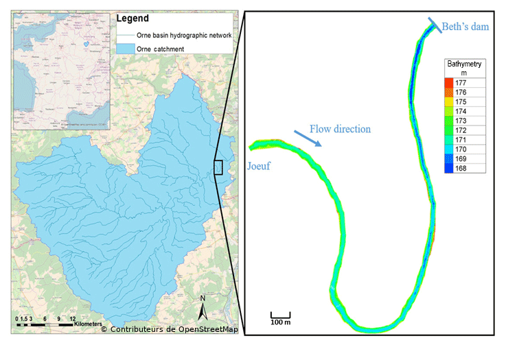
Figure 1Study area and model domain (4 km long control section of the Orne river). © OpenStreetMap contributors 2019. Distributed under a Creative Commons BY-SA License.
3.2 Available data
Since January 2014, we have concentrated the monitoring efforts on continuously recording streamflow and water turbidity as a proxy of SSC. Moreover, we monitored bathymetry (i.e. riverbed elevation) episodically at selected locations on the riverbanks and the riverbed. The continuous data used in this study were acquired during a moderate-magnitude flood event that occurred in March 2017. During this event, a peak discharge of 45 m3 s−1 was recorded, and the turbidity did not exceed 150 NTU (Fig. 2).
3.2.1 Suspended sediment concentration
SSC is generally measured occasionally, whereas models require continuous input data time series. In this context, turbidity is often recognized as a good proxy for assessing the continuous time series of SSC (Martínez-Carreras et al., 2016). In this study, turbidity was measured every 5 min at the downstream boundary using a YSI 600 OMS turbidimeter. During the flood event that occurred in March 2017, turbidity values ranged from 0 to 150 NTU. These measurements are used to calibrate the relationship between turbidity and SSC (Fig. 2). The polynomial regression between the two datasets (e.g. Versini et al., 2015) exhibits Pearson's correlation coefficient of 0.968 and a residual mean of 1.44 mg L−1 (Fig. 2).
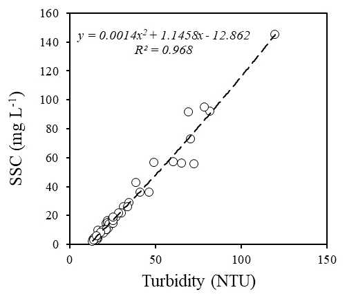
Figure 2Relationship between the river water turbidity and suspended sediment concentration (SSC) measured at the downstream boundary of the model domain (monitoring period: 1–14 March 2017; n=31).
Water samples were collected every 6 h using ISCO© automatic samplers at the upstream and downstream boundaries. The similarities between measured and estimated SSC at both locations (Fig. 3) indicate that the sampling frequency is sufficient for capturing the suspended sediment dynamics in the river section during this event. As a consequence, the interpolation of the SSC punctual measurements at the upstream boundary is used as an upstream forcing of the model. The SSC was measured by filtering 0.5 L of river water through 1.2 µm Whatman GF/C glass fibre filters by means of a Millipore vacuum pump. All filters were previously dried at 105 ∘C for 24 h, cooled in a desiccator, and weighted. After filtration, the filters were dried again at 105 ∘C and reweighted. The differences between weightings provided the total amount of sediment retained in the filters. We calculated the SSC by dividing the total amount of sediment retained in the filters by the volume of the filtered samples.
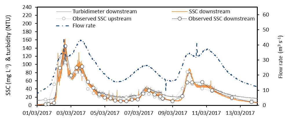
Figure 3Times series of flow rate, turbidity, and calculated SSC. Punctual SSC measured at the upstream and downstream boundaries of the model domain is also plotted for comparison.
3.2.2 Sediment grain-size distribution

Figure 4Sediment grain-size distributions estimated from the Orne river sediment samples collected in (a) the riverbed and (b) the riverbanks (average value over nine samples collected at three different river stations).
We estimated the grain-size distributions shown in Fig. 4 by sieving dried sediment samples collected in three different areas of the river section. Due to deep water at the downstream end of the river section caused by the dam, it was technically impossible to collect riverbed sediments in this part of the river. Moreover, as an extensive sampling of sediments along the river was not feasible, we assumed, as an initial condition of the model simulations, that the riverbed and riverbank sediment grain-size distributions were homogeneous along the river reach. Initial sediment grain-size distributions were estimated by averaging the three sediment samples.
3.2.3 Sediment density
In sediment transport modelling, the density of the sediment is usually set to 2600 kg m−3 (Van Rijn, 1989). Here, we suggest considering a measured sediment density for each sediment class. To this end, we measured the variation in water volume in a 400 mL graduated flask while pouring a predefined mass of sediment into the water. The density measurements exhibit a spread of 1000 kg m−3 and an average value of 2300 kg m−3. The minimum density is 1800 kg m−3 for the 63 µm sediment class (Fig. 5).
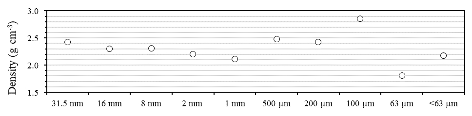
Figure 5The Orne riverbed sediment density measured for each of the 10 sediment size classes.
3.2.4 Riverbed bathymetry
The bathymetry of the riverbed and the lower part of the banks was carried out during two field campaigns (in summer 2015 and summer 2016) using a differential global navigation satellite system (GNSS; vertical accuracy of ca. 1 mm) coupled with an echo sounder (vertical accuracy of ca. 1 mm). The ground elevation of the upper parts of the banks was measured using a differential GNSS (vertical accuracy of ca. 1 mm) and a total station (vertical accuracy of ca. 1 cm) when the GNSS signal was not accurate enough due to the dense vegetation cover. These campaigns allowed us to measure riverbed elevation along the river cross section around every 100 m.
3.3 Model set-up and experimental design
Particularly well-adapted to simulate river hydrodynamics, TELEMAC-MASCARET is based on a finite-element unstructured mesh, allowing the representation of complex geometries (Hostache et al., 2014). For the study area, the unstructured mesh is composed of 16 492 nodes. The distance between neighbour nodes ranges between 7 and 25 m. It was generated using POLYMESH@ (developed by A. Roland, TU Darmstadt). The six bridge pillars located in the domain are represented in the model geometry. The riverbed and riverbank sediments are defined with two different grain-size distributions (Fig. 4).
We designed four model configurations to assess the influence of sediment grain-size distribution, sediment particle density, and the SSC boundary condition on model predictions (Table 1). The SISYPHE and TELEMAC-3D parameter values remain identical for the four different modelling configurations. The SSC distribution is assumed to be equal to the distribution of the erosion fluxes of each class at the boundary conditions. The settling velocity is calculated for each sediment class using the experimental sediment density values (Eq. 7 and Fig. 5). Moreover, due to the presence of vegetation on the riverbanks, the corresponding apparent roughness is fixed at 4 cm for the four modelling set-ups.

The first configuration (2CL) corresponds to the standard SISYPHE configuration, which only considers two classes of particle sizes with distinct densities. The second configuration (10CL) considers a riverbed bottom sediment composed of 10 classes with distinct density values (Fig. 5) and an input SSC, at the upstream boundary condition, distributed over the same 10 classes. The third configuration (10CLD) differs from the 10CL configuration in terms of sediment density: the 10 sediment classes have the same “standard” density value (i.e. 2600 kg m−3). Note that the standard density value is higher than the values we measured in the laboratory for all the sediment classes except for the 100 µm class (2850 kg m−3; Fig. 5). The last configuration (10CL1CS) is identical to the 10CL configuration except that the input SSC is imposed only on the sediment with the smallest particle size (<5 µm).
In this section, we present, evaluate, and discuss our results based on the four model configurations (Table 1). In particular, we aim to evaluate the influence of the sediment size distribution, sediment density, and representation of the upstream boundary conditions on the simulated SSC and bed evolution, respectively. To carry out this evaluation, the simulated SSC at the downstream boundary of the model domain is first compared with the corresponding measured data.
4.1 Evaluation of the simulated SSC
4.1.1 Influence of the sediment grain-size distribution
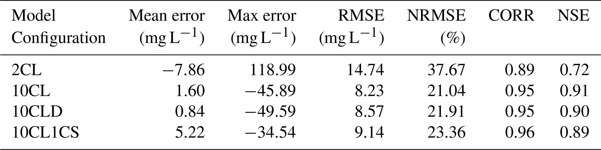
The 2CL configuration required some additional effort for the model initialization and spin-up. Indeed, without a numerical adjustment of the initial bathymetry, the 2CL configuration was unable to provide a satisfying fit with the measured SSC data as spurious fluxes of SSC appeared (Fig. 6a). Some authors (e.g. Waeles, 2005) reported the need for long-term simulations (up to 1 year) in order to obtain a satisfactory initial state of the bathymetry and the sediment repartition. In our study, we successively simulated the same event several times. Five iterations (referred to as 2CL1–2CL5) were necessary in order to stabilize the initial bathymetry and avoid a systematic overestimation of the first SSC peaks (Fig. 6a and b). We took the fifth run of the 2CL configuration (i.e. 2CL5) as a reference, as it yielded the best results in terms of simulated SSC. Model initialization and spin-up were not necessary for the other configurations, namely 10CL, 10CLD, and 10CL1CS.
Table 2 shows that better model performances are yielded when using a larger number of grain-size classes. Indeed, not only are the error metrics substantially reduced in the 10CL configuration (in comparison to the 2CL5 configuration) but Pearson's correlation coefficient and the Nash–Sutcliffe efficiency (NSE) are also significantly increased. Moreover, as shown in Fig. 6, the 2CL5 configuration tends to overestimate the first SSC peak (maximum absolute error: 118 mg L−1) and underestimate SSC for the rest of the simulation (mean error: −7 mg L−1). This highlights the limitations of a 2-class model that is not able to correctly predict SSC both at rather low and high flows. On the contrary, the 10CL configuration is able to capture the SSC accurately, as the mean and the maximum errors are 1.6 and −45 mg L−1, respectively.
4.1.2 Influence of the sediment density
As a reminder, in the 10CL model configuration, we use distinct densities for each class of sediment (Fig. 5), whereas in 10CLD, we use a unique value of density (2600 kg m−3). During the simulated event, the contribution of the non-cohesive sediment to the SSC is limited (ca. 1 mg L−1 at maximum). Both configurations reproduce the measured SSC (Fig. 6c) accurately. However, the 10CL configuration slightly outperforms 10CLD (Table 2), as the peaks of SSC are better predicted. Moreover, a substantial difference between the two model simulations is observed at the first and last peak of SSC (10 mg L−1; representing ca. 10 % of the last SSC peak). The fall velocities are directly linked to the density (Eq. 6). As a result, overestimating sediment density can significantly reduce simulated SSC. In our study, the effect of sediment density on model results is nevertheless slightly limited due to the rather low magnitude of the simulated flood event. We would certainly expect the effect of using measured nominal sediment densities to have a larger positive effect on simulated SSC time series when simulating larger flood events, as larger sediment classes would be transported.
In this sediment transport modelling study, we chose to consider an average density value of 2600 kg m−3 in the 10CLD scenario, as this is the most commonly used value. One could argue that the average measured sediment density could also perform satisfactorily. To evaluate this option, we carried out an additional simulation identical to 10CLD but using a sediment density of 2300 kg m−3 (results not shown). The results obtained were similar to those obtained with the 10CLD configuration and different from the 10CL simulations, showing the added value of using nominal measured densities. This is arguably mainly due to the fact that only fine sediment classes are transported during this flood event and that fine sediment classes have different nominal densities than the tested average values, namely 2300 and 2600 kg m−3 (see Fig. 5).
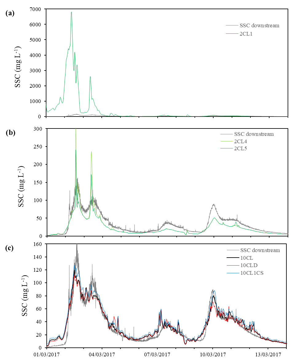
Figure 6Simulated and measured suspended sediment concentration time series at the downstream boundary for configurations (a) 2CL (first run); (b) 2CL (fourth and fifth runs); and (c) 10CL, 10CLD, and 10CL1CS. SSC: suspended sediment concentration. 10CL, 10CLD, 10CL1CS, 2CL1, 2CL4, and 2CL5: various modelling scenarios (please refer to Table 1).
Table 2Model performances computed for a 14 d simulation period (1–14 March 2017). NRMSE is the normalized root-mean-square error, and CORR is correlation.
4.1.3 Influence of the suspended sediment size distribution at the upstream boundary
The simulated SSC is generally higher in the 10CL1CS scenario than in the 10CL (Fig. 6c). This is mainly due to the way in which the upstream SSC is imposed in the 10CL configuration (i.e. distributed over 10 classes). As a result, coarser particles tend to settle more rapidly, and the predicted SSC downstream is lower than in the 10CL1CS configuration. Overall, the error metrics and the skill scores reported in Table 2 show that the 10CL configuration slightly outperforms the 10CL1CS configuration, as errors are lower and the NSE is slightly higher.
Figure 3 shows that the SSC time series have similar shapes and magnitudes at the upstream and downstream boundaries of the model. This indicates that erosion plays a limited role in the overall sediment transport budget when compared to advection and dispersion during this rather low-magnitude flood event. To further investigate this, Fig. 7 shows the cumulative (starting from larger grain size) distribution of the SSC per sediment class simulated at the downstream boundary by the 10CL and 10CL1CS configurations. The contribution of non-cohesive sediments to the overall SSC is rather limited (in the order of 1 mg L−1 at maximum) and only contains the 100 µm sediment class for both models. However, as is visible in Fig. 7b, the 63 and 30 µm sediment classes are transported in the 10CL1CS configuration. This result shows that erosion within the domain contributes slightly to the sediment transport budget because these classes are not introduced into the model domain via the upstream boundary condition. Moreover, as these two configurations yield markedly different results in terms of suspended sediment size distribution (Fig. 7), the way the upstream boundary condition is defined is shown to have significant importance, especially on the advection and diffusion processes.
It is also worth mentioning that larger differences between the two configurations are expected in terms of simulated SSC for higher-magnitude flood events. Indeed, for such flood events, larger sediment particles are transported as a result of higher flow velocities. Distributing the upstream SSC over various sediment classes would then allow the transport of larger sediment particles via advection–dispersion in configuration 10CL.
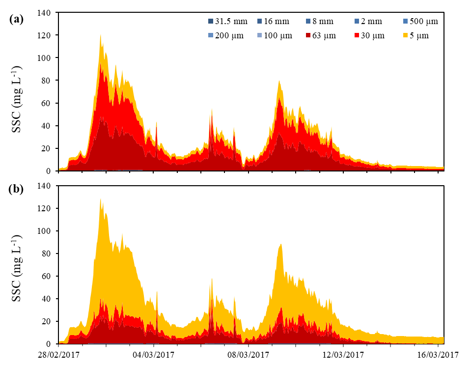
Figure 7Downstream suspended sediment grain-size cumulative distribution simulated by model configurations (a) 10CL and (b) 10CL1CS.
4.2 Cross-comparison of simulated riverbed evolution
Comparing simulated bathymetry evolution maps showing changes in riverbed elevation is not straightforward for a moderate-magnitude event on a small river. This is especially true because the evolutions are rather limited and local, and it is difficult to collect sufficiently accurate ground-truth data. To facilitate such a comparison, the evolutions of the riverbed elevation simulated by the various model configurations are compared via scatter plots (Fig. 8) using the 10CL configuration as a reference. Using bathymetry evolution instead of bathymetry itself not only allows a differentiation between erosion and deposition but also an assessment of the thickness of deposited and eroded material. The bathymetry evolutions simulated by the 10CL configuration are separated as follows: erosion area (elevation change <−5 mm), stable area (elevation change in [−5 mm : 5 mm]), and deposition area (elevation change >5 mm).
4.2.1 Influence of the sediment grain-size distribution
The comparison between evolutions obtained with the 2CL and 10CL configurations shows very low correlation coefficients (0.17 and 0.02 for erosion and deposition, respectively). Moreover, stable areas in the 10CL configuration are unstable in the 2CL configuration (−0.11 of correlation). These substantial differences between the two configurations confirm that the number of sediment size classes implemented in the model plays a central role in the simulation of erosion–deposition processes. Overall, riverbed evolutions simulated by the 2CL model configuration are very limited. This is mainly attributed to the model spin-up that was necessary for stabilizing the bathymetry (see Sect. 3.1). The simplified sediment size distribution (two classes) artificially amplifies the availability of the finest sediment class. This leads to a washout of this class during the spin-up simulation and at the beginning of the simulation.
4.2.2 Influence of the sediment density
The middle scatter plot in Fig. 8 shows a good correlation between riverbed evolutions simulated by the 10CL and 10CLD configurations. The correlation coefficients between erosion and deposition areas computed with both configurations are high, with respective values of 0.97 and 0.92. Moreover, we argue that the influence of sediment density on model simulations would be larger when simulating higher-magnitude flood events, as the range of transported sediment sizes would be broader. Indeed, during larger flood events, we might expect that coarser sediments are transported, eroded and deposited. Moreover, a change in sediment density is associated with a change in fall velocity, which implies changes in the transport processes: a higher density reduces transport, and, on the contrary, a lower density increases it. Changes in density would therefore also result in the displacement of erosion and deposition areas for coarser sediment, making bathymetry evolutions more markedly different in 10CL and 10CLD configurations during higher-magnitude flood events.
4.2.3 Influence of the suspended sediment size distribution at the upstream boundary
The right scatter plot in Fig. 8 shows a good correlation between the10CL1CS and 10CL configurations in terms of deposition and erosion areas, with respective values of 0.99 and 0.98. As previously argued, the differences in bathymetry evolution between the two configurations would likely be more important in the event of a higher flow rate.
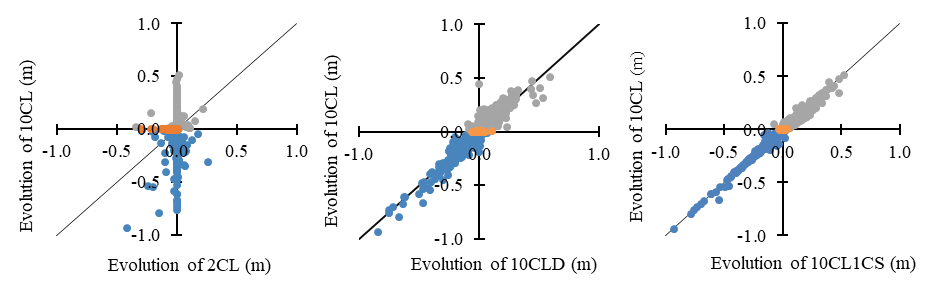
Figure 8Cross-comparison of bed elevation evolutions (elevation final–initial) simulated for the 2CL, 10CL1CS, and 10CLD configurations using the model configuration 10CL as a reference. The colours correspond to the 10CL's bathymetry evolution: grey is the deposition, orange is the stable bathymetry, and blue is the erosion.
4.3 Cross-comparison of simulated bottom-sediment median grain-size evolution
To further analyse the differences between the various modelling configurations, we propose cross comparing the evolutions of riverbed sediment median grain size at each model grid node. The 10CL configuration is again used as a reference.
4.3.1 Influence of sediment grain-size distribution
Figure 9 (left-hand-side panel) shows very limited correlation between the D50 evolutions when using the 10CL and the 2CL configurations (correlation coefficient of −0.05). The median evolution of the D50 in the whole area when using the 2CL configuration is about 70 µm: the fine particles tend to leave the domain and the D50 increases. On the contrary, the median evolution of the D50 when using the 10CL configuration is close to zero: there is an equilibrium of the D50 in the domain, indicating that the local grain-size evolution during the event does not modify the median D50 over the domain.
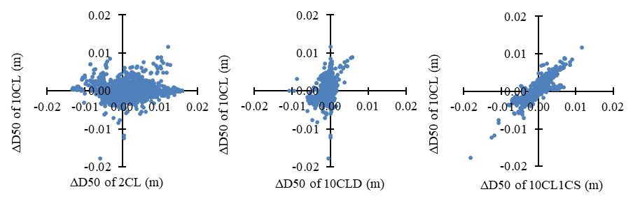
Figure 9Cross-comparison of riverbed sediment median grain-size evolution (final–initial) simulated using the 2CL, 10CL1CS, and 10CLD configurations using the 10CL configuration as a reference.
4.3.2 Influence of the sediment density
Figure 9 (centre panel) shows limited correlation between D50 evolutions when using the 10CL and 10CLD configurations (correlation coefficient of 0.32). This shows that sediment density substantially influences bottom-sediment grain-size evolution. The scatter plot exhibits a higher variance along the vertical axis (10CL configuration), indicating a more limited sediment grain-size evolution for the 10CLD configuration. The use of nominal sediment densities tends to increase the evolution of D50 during the flood event.
4.3.3 Influence of the suspended sediment size distribution at the upstream boundary
Figure 9 (right-hand-side panel) shows a high correlation between the D50 evolutions in the 10CL and 10CL1CS configurations (correlation coefficient of 0.87). The median evolution of the bottom-sediment D50 (over the whole area) in the 10CL1CS configuration is also close to zero, suggesting that there is an equilibrium of the D50 all over the domain, as in the 10CL configuration. This particular flood event was of moderate magnitude. Consequently, the fraction of suspended fine sand imposed at the upstream boundary condition in the 10CL configuration was negligible, and the suspended sediment was mainly composed of the three cohesive sediment classes. Hence, the differences between 10CL and 10CL1CS are limited due to the moderate magnitude of the flood event.
This study evaluates the influence of the sediment grain-size distribution, the sediment density, and the upstream SSC representation in sediment transport and morphodynamic modelling. In this context, we further developed the SISYPHE model to integrate 10 classes of sediment (mixture of cohesive and non-cohesive sediment) with individual sediment densities (two sediment classes are implemented in the standard version). The physical parameterization has also been rewritten, based on the parameterization proposed by Lepesqueur (2009), and has been adapted to the last release of SISYPHE (i.e. from version V5P8 to V7P7). The enhanced SISYPHE model is evaluated using a moderate-magnitude flood event that occurred in a small river (the Orne river in north-eastern France) as a test case.
The following conclusions are drawn from this study:
-
The simulated suspended sediment concentration (SSC) is markedly improved if the model takes into account 10 sediment classes instead of 2. The RMSE in SSC is reduced by a factor of 2 with 10 sediment classes. The simplified model with only two sediment classes appeared to simulate spurious sediment fluxes. Considering 2 or 10 classes of sediment in the model results in markedly different erosion–deposition areas.
-
The sediment density substantially influences model results, albeit to a smaller extent. Using a measured sediment density for each sediment class instead of a standard uniform value (i.e. 2600 kg m−3) allowed for a slight gain in the model performance compared to simulated SSC. Our analysis, based on a correlation of riverbed evolutions, also shows that using measured sediment densities instead of standard ones slightly changes the areas of erosion–deposition.
-
The way in which the input SSC is introduced at the upstream boundary also plays a role in the model performance, albeit a limited one in the simulated flood event. This was found to mainly influence advection–dispersion processes, whereas the influence on erosion–deposition was not significant.
The proposed sediment transport modelling framework is found to improve the accuracy of the results. However, additional developments could be considered in order to integrate bio-physicochemical processes. Indeed, the temporal variability in the bio-physicochemical conditions in rivers plays a key role in shaping the sediment dynamics during flood events. In this context, we envisage implementing two important developments:
-
A new generation of high-frequency measurement sensors could be used to record the model input data. A LISST sensor (Fugate and Friedrichs, 2002), which measures the size and concentration of particles suspended in water, or a combination of two acoustic doppler current profilers (Jourdin et al., 2014), could for example be used to monitor the SSC for each individual sediment class. This would provide more realistic model inputs and more accurate validation data at the same time.
-
Flocculation processes could be integrated, as they play a key role in sediment transport due to the fact that the density and the shape of flocs differ from those of individual sediment particles. As a result, their displacement in the water column is different from that of isolated sediment particles (Parker, 1972; Van der Lee, 2009). The integration of flocculation process could be implemented by coupling a morphodynamic model with a floc population model such as FLOCMOD (Verney et al., 2009; Lepesqueur et al., 2018).
In terms of longer-term developments, the erosion and deposition laws used in the morphodynamic model should also take into account interactions between sediment classes, as argued for example by Starck (2014). Indeed, many existing studies highlight the importance of the compaction of non-cohesive sediment (Swidersky, 1976), armouring (Egiazaroff, 1965), hiding and exposure (Ashida, 1973), filtration of fine particles by coarser sediment (Karim, 1982; Brunke, 1999; Herzig et al., 1970), and lubrication (Barry, 2006) together with biological processes (e.g. Athur et al., 1981; Widdows et al., 2000; Le Hir et al., 2007).
All the datasets related to the MOBISED project and, more specifically, the dataset of this paper (https://doi.org/10.24396/ORDAR-27; Hissler, 2019) are fully accessible and can be directly download on the platform OTELO from the University of Lorraine (https://doi.org/10.17616/R3F19K; re3data.org, 2019).
JL wrote the paper, with support from RH, NMC, EMP, and CH. All of these authors contributed to the design of the experiment and the analysis of the results. JL implemented the further developments of the Telemac hydroinformatic system.
The authors declare that they have no conflict of interest.
This study is part of the MOBISED project. We would like to thank Jean-François Iffly, Jérôme Juilleret, Luc Manceau, and Cyrille Taillez for the maintenance of field equipment and the accurate field data acquisition and Claire Delus and Benoît Losson for the constructive scientific discussions related to hydrological and sedimentary issues in the Orne river basin.
This research has been supported by the Luxembourg National Research Fund (FNR) and the French National Research Agency (ANR) in the framework of the FNR INTER-ANR research programme (contract no. INTER/ANR/13/9441502).
This paper was edited by Erwin Zehe and reviewed by three anonymous referees.
Ashida, K. and Mishiue, M.: Studies on bed load transport rate in alluvial streams, Trans JSCE, 1973.
Athur, R. M., Nowell, A. R. M., Jumars, P. A., and Eckman, J. E.: Effects of biological activity on the entrainment of Marine sediments, Mar. Geol., 42, 133–153, 1981.
Barrière, J., Oth, A., Hostache, R., and Krein, A.: Bedload transport monitoring using seismic observations in a low-gradient rural gravel-bed stream, Geophys. Res. Lett., 42, 2294–2301, https://doi.org/10.1002/2015GL063630, 2015.
Barry, K. M., Thieke, R. J., and Mehta, A. J.: Quasi-hydrodynamic lubrication effect on clay particles on sand grain erosion, Estuar. Coast. Shelf S., 67, 161–169, 2006.
Belleudy, P.: Modelling of deposition of sediment mixtures, part 1: analysis of a flume experiment, J. Hydraul. Res., 38, 417–425, 2000.
Belleudy, P: Modelling of deposition of sediment mixtures, part 2: a sensitivity analysis, J. Hydraul. Res., 39, 25–31, 2001.
Brunke, M.: Colmatin and Depth filtration within streambed: retention of particles in hyportheic interstices, Int. Rev. Hydrobiol., 84, 99–117, https://doi.org/10.1002/iroh.199900014, 1999.
Carter, J., Walling, D., Owens, P., and Leeks, G.: Spatial and temporal variability in the concentration and speciation of metals in suspended sediment transported by the River Aire, Yorkshire, UK, Hydrol. Process., 20, 3007–3027, 2006.
Celik, I. and Rodi, W.: Modelling suspended sediment transport in nonequilibrium situations, J. Hydrol. Eng., 114, 1157–1119, 1988.
Durafour, M., Jarno, A., Le Bot, S., Lafite, R., and Marin, F.: Bedload transport for heterogenous sediments, in: Evironmental Fluid Mechanics, Springer Verlag, 15, 731–751, https://doi.org/10.1007/s10652-014-9380-1, 2015.
Egiazaroff, I. A.: Calculation of non-uniform sediment concentrations, J. Hydr. Eng. Div.-ASCE, 91, 225–247, 1965.
Exner, F. M.: Zur Physik der Dünen, Akad. Wiss. Wien Math. Naturwiss. Klasse, 129, 929–952, 1920.
Exner, F. M.: Über die Wechselwirkung zwischen Wasser und Geschiebe in Flüssen, Akad. Wiss. Wien Math. Naturwiss. Klasse, 134, 165–204, 1925.
Fugate, D. C. and Friedrichs, C. T.: Determining concentration and fall velocity of estuarine particle populations using ADV, POBS and LISST, Cont. Shelf Res., 22, 1867–1886, 2002.
García Alba, J., Gómez, A. G., Tinoco López, R. O., Sámano Celorio, M. L., García Gómez, A., and Juanes, J. A.: A 3-D model to analyze environmental effects of dredging operations – application to the Port of Marin, Spain, Adv. Geosci., 39, 95–99, 2014.
González-Sanchis, M., Murillo, J., Cabezas, A., Vermaat, J. E., Comín, F. A., and García-Navarro, P.: Modelling sediment deposition and phosphorus retention in a river floodplain, Hydrol. Process., 29, 384–394, https://doi.org/10.1002/hyp.10152, 2014.
Grabowski, R. C., Droppo, I. G., and Wharton, G.: Erodibility of cohesive sediment: The importance of sediment properties, Earth-Sci. Rev., 105, 101–120. https://doi.org/10.1016/j.earscirev.2011.01.008, 2011.
Guillou, N. and Chapalain, G.: Numerical simulation of tide-induced transport of heterogeneous sediments in the English Channel, Cont. Shelf. Res., 30, 806–819, https://doi.org/10.1016/j.csr.2010.01.018, 2010.
Heise, S. and Förstner, U.: Risks from historical contaminated sediments in the Rhine basin, Water Air Soil Pollut., 6, 261–272, 2006.
Heise, S. and Förstner, U.: Risk assessment of contaminated sediments in river basins – theoretical considerations and pragmatic approach, J. Environ. Monit., 9, 943–952, 2007.
Hervouet, J. M.: Hydrodynamics of Free Surface Flows, John Wiley and Sons, USA, 2007.
Herzig, J. P., Leclerc, D. M., and Legoff, P.: Flow suspension through porous media – application to deep bed filtration, Industrial Engineering Chem., 62, 9–35, 1970.
Hissler, C.: Dataset related to the publication from Lepesqueur et al. (2019), OTELO, https://doi.org/10.24396/ORDAR-27, 2019.
Hissler, C. and Probst, J.-L: Chlor-alkali industrial contamination and riverine transport of mercury: Distribution and partitioning of mercury between water, suspended matter, and bottom sediment of the Thur River, France, Appl. Geochem., 21, 1837–1854, 2006.
Hissler, C., Hostache, R., Iffly, J.-F., Pfister, L., and Stille, P.: Anthropogenic rare earth element fluxes to floodplains: coupling between geochemical monitoring and hydrodynamic-sediment transport modelling, C. R. Geosci., 347, 294–303, 2015.
Hostache, R., Hissler, C., Matgen, P., Guignard, C., and Bates, P.: Modelling suspended-sediment propagation and related heavy metal contamination in floodplains: a parameter sensitivity analysis, Hydrol. Earth Syst. Sci., 18, 3539–3551, https://doi.org/10.5194/hess-18-3539-2014, 2014.
Jacobs, W., Le Hir, P., Van Kesteren, W. G. M., and Cann, P.: Erosion threshold of sand-mud mixtures, Cont. Shelf Res., 31, 14–25, https://doi.org/10.1016/j.csr.2010.05.012, 2011.
Jourdin, F., Tessier, C., Le Hir, P., Verney, R., Lunven, M., Loyer, S., Lusven, A., Filipot, J.-F., and Lepesqueur, J.: Dual-frequency ADCPs measuring turbidity, Geo.-Mar. Lett., 34, 381–397, 2014.
Kanbar, H. J., Montargès-Pelletier, E., Losson, B., Bihannic, I., Gley, R., Bauer, A., Villieras, F., Manceau, L., El Samrani, A. G., Kazpard, V., and Mansuy-Huault, L.: Iron mineralogy as a fingerprint of former steelmaking activities in river sediments, Sci. Total Environ., 599–600, 540–553, 2017.
Karim, M. F. and Kennedy, J. F.: A computer based flow and sediment routing, IIH Report N250, 1965.0, Iowa Institute of Hydraulic Research, University of Iowa, Iowa City, Iowa, 1982.
Krone, R. B.: Flume studies of the transport of sediment in estuarial shoaling processes, University of California Hydraulic Eng. and Sanitary Eng. Res. Lab. Berkeley, California, 110 pp., 1962.
Le Hir, P., Monbet, Y., and Orvain, F.: Sediment erodability in sediment transport modelling: Can we account for biota effects?, Cont. Shelf Res., 27, 1116–1142, 2007.
Le Hir, P., Cayocca, F., and Waeles, B.: Dynamics of sand and mud mixtures: A multiprocess-based modelling strategy, Cont. Shelf Res., Supplement, 31, S135–S149, 2011.
Lepesqueur, J., Chapalain, G., Guillou, N., and Villaret, C.: Quantification des flux sédimentaires dans la rade de Brest et ses abords, 31 émes Journées de l'Hydraulique de la SHF: Morphodynamique et gestion des sédiments dans les estuaires, les baies et les deltas, SHF, Paris, 2009.
Lepesqueur, J., Hostache, R., Martínez-Carreras, N., Manceau, L., Delus, C., Losson, B., Montarges-Pelletier, E., and Hissler, C.: A hydro-morphodynamic model integrating extended sediment particle size distribution and flocculation processes for better simulating hydro-sedimentary fluxes, E3S Web of Conferences, Volume 40, 5 September 2018, Article number 050259, International Conference on Fluvial Hydraulics, River Flow 2018, Lyon-Villeurbanne, France, 2018.
Martínez-Carreras, N., Schwab, M. P., Klaus, J., and Hissler, C.: In situ and high frequency monitoring of suspended sediment properties using a spectrophotometric sensor, Hydrol. Process., 30, 3533–3540, https://doi.org/10.1002/hyp.10858, 2016.
Miedima, S. A.: Constructing the Shields curve, a new theoretical approach and its applications, WODCON XIX, Beijing China, 2010.
Mignot, C.: Tassement et rhéologie des vases, 1re partie, Revue Internationale La Houille Blanche, 1, SHF, Paris, 1989.
Mitchener, H. and Torfs, H.: Erosion of sand/mud mixtures, J. Coastal Eng., 29, 1–25, 1996.
Nikuradse, J.: Gesetzmässigkeiten der Turbulente Strömung in Glatten Rohren, Ver. Deut. Ing. Forschungsheft, 356, Ver. Deut. Ing. Forschungsheft, Düsseldorf, 1932.
Panagiotopoulos, I., Voulgaris, G., and Collins, M. B.: The influence of clay on the threshold of movement of fine sandy beds, Coast. Eng., 32, 19–43, 1997.
Parker, D. S., Kaufman, W. J., and Jenkins, D.: Floc break-up in turbulent flocculation processes, J. Sanitary Eng. Div., 98, 79–99, 1972.
Partheniades, E.: Erosion and deposition of cohesive soils, J. Hydr. Eng. Div.-ASCE, 91, 105–139, 1965.
Qilong, B. and Toorman, E. A: Mixed-sediment transport modelling in Scheldt estuary with a physics-based bottom friction law, Ocean Dynam., 65, 555–587, https://doi.org/10.1007/s10236-015-0816-z, 2015.
re3data.org: ORDaR; editing status 2019-01-30; re3data.org – Registry of Research Data Repositories, https://doi.org/10.17616/R3F19K, 2019.
SedNet: The SEDNET strategy paper. The opinion of SedNet on environmentally, socially, and economically viable sediment management, TNO, the Netherlands, 22 pp., 2003.
Shields, A.: Anwendung der Aehnlichkeitsmechanik und der Turbulenzforschung auf die Geschiebebewegung, Mitteilungen der Preußischen Versuchsanstalt für Wasserbau, 26, Preußische Versuchsanstalt für Wasserbau und Shiffbau, Berlin, 1936.
Smith, J. and McLean, S.: Spatially averaged flow over a wavy surface, J. Geophys. Res., 82, 1735–1746, 1977.
Soulsby, R.: Dynamics of marine sands, Thomas Telford Publishing, London, 249 pp., 1997.
Soulsby, R. and Whitehouse, R.: Threshold of sediment motion in coastal environment, Proceedings Pacific Coasts and Ports, 149–154, University of Canterbury, Christchurch, New Zealand, 1997.
Stark, N., Hay, A. E., Cheel, R., and Lake, C. B.: The impact of particle shape on the angle of internal friction and the implications for sediment dynamics at a steep, mixed sand–gravel beach, Earth Surf. Dynam., 2, 469–480, https://doi.org/10.5194/esurf-2-469-2014, 2014.
Swidersky, R. E.: The effect of angularity on the compaction and shear strength of cohesionless material, Master thesis, New Jersey institute of technology, Newark, 1976.
Van der Lee, E. M., Bowers, D. G., and Kyte, E.: Remote sensing of temporal and spatial patterns of suspended particle size in the Irish Sea in relation of the Komolgorov microscale, Cont. Shelf Res., 29, 1213–1225, 2009.
Van Ledden, M.: Modelling of sand-mud mixtures. Part II: A process-based sand mud model. WL | DELFT HYDRAULICS (Z2840), TU Delft, Delft, 2001.
Van Rijn, L. C.: Hand book Sediment Transport by currents and waves, Delft Hydraulics, Rep. H461, TU Delft, Delft, 1989.
Verney, R., Lafite, R., and Brun-Cottan, J.: Flocculation potential of estuarine particles: the importance of environmental factors and of the spatial and seasonal variability of suspended particulate matter, Estuar. Coasts, 32, 670–693, 2009.
Versini, P. A., Joannis, C., and Chebbo, G.: Onema, LEESU et IFSTTAR/LEE: Guide technique sur le mesurage de la turbidité dans les réseaux d'assainissement, Onema, Vincennes, 2015.
Villaret, C.: Sisyphe user manual, Tech. Rep., EDF R&D, Chatou, 2010.
Villaret, C., Hervouet, J. M., Kopmann, R., Merkel, U., and Davies, A. G.: Morphodynamic modelling using the Telemac finite-element system, Comput. Geosci., 53, 105–113, 2013.
Waeles, B.: Modélisation morphodynamique de l'embouchure de la Seine, Phd Thesis, University of Caen, France, 2005.
Warner, J. C., Armstrong, B., He, R., and Zambon, J. B.: Development of a Coupled Ocean–Atmosphere–Wave–Sediment Transport (COAWST) Modeling System, Ocean Model., 35, 230–244, https://doi.org/10.1016/j.ocemod.2010.07.010, 2010.
Widdows, J., Brinsley, M. D., Salked, P. N., and Lucas, C. H.: Influence of biota on spatial and temporal variation in sediment erodability and material flux on tidal flat (Westerschelde, the Netherlands), Mar. Ecol. Prog. Ser., 194, 23–37, 2000.
Whitman, W. B., Coleman, D. C., and Wiebe, W. J.: Prokaryotes: the unseen majority, P. Natl. Acad. Sci. USA, 95, 6578–6583, 1998.
Zanke, U.: Berechnung der Sinkgeschwindigkeiten von Sedimenten, Vol. 46, Mitteilungen Franzius Institute Univ. Hannover, Hannover, 1977.
Zanke, U. C. E.: On the influence of turbulence on the initiation of sediment motion, Int. J. Sediment. Res., 18, 17–31, 2003.