the Creative Commons Attribution 4.0 License.
the Creative Commons Attribution 4.0 License.
 | 13 Sep 2019
Water restrictions under climate change: a Rhône–Mediterranean perspective combining bottom-up and top-down approaches
Bastien Richard
Alexandre Devers
Christel Prudhomme
Drought management plans (DMPs) require an overview of future climate conditions for ensuring long-term relevance of existing decision-making processes. To that end, impact studies are expected to best reproduce decision-making needs linked with catchment intrinsic sensitivity to climate change. The objective of this study is to apply a risk-based approach through sensitivity, exposure and performance assessments to identify where and when, due to climate change, access to surface water constrained by legally binding water restrictions (WRs) may question agricultural activities. After inspection of legally binding WRs from the DMPs in the Rhône–Mediterranean (RM) district, a framework to derive WR durations was developed based on harmonized low-flow indicators. Whilst the framework could not perfectly reproduce all WR ordered by state services, as deviations from sociopolitical factors could not be included, it enabled the identification of most WRs under the current baseline and the quantification of the sensitivity of WR duration to a wide range of perturbed climates for 106 catchments. Four classes of responses were found across the RM district. The information provided by the national system of compensation to farmers during the 2011 drought was used to define a critical threshold of acceptable WR that is related to the current activities over the RM district. The study finally concluded that catchments in mountainous areas, highly sensitive to temperature changes, are also the most predisposed to future restrictions under projected climate changes considering current DMPs, whilst catchments around the Mediterranean Sea were found to be mainly sensitive to precipitation changes and irrigation use was less vulnerable to projected climatic changes. The tools developed enable a rapid assessment of the effectiveness of current DMPs under climate change and can be used to prioritize review of the plans for those most vulnerable basins.
- Article
(8551 KB) - Full-text XML
- BibTeX
- EndNote


The Mediterranean region is known as one of the “hotspots” of global change (Giorgi, 2006; Paeth et al., 2017) where environmental and socio-economic impacts of climate change and human activities are likely to be very pronounced. The intensity of the changes is still uncertain; however, climate models agree on a significant future increase in frequency and intensity of meteorological, agricultural and hydrological droughts in southern Europe (Jiménez Cisneros et al., 2014; Touma et al., 2015), with climate change likely to exacerbate the variability in climate with regional feedbacks affecting Mediterranean-climate catchments (Kondolf et al., 2013). Facing more severe low flows and significant losses of snowpack, southeastern France will be subject to substantial alterations of water availability; Chauveau et al. (2013) have shown a potential increase in low-flow severity by the 2050s with a decrease in low-flow statistics to 50 % for the Rhône river near its outlet. Andrew and Sauquet (2017) have reported that global change will most likely result in a decrease in water resources and an increase both in pressure on water resources and in occurrence of periods of water limitation within the Durance river basin, one of the major water towers of southeastern France. In addition, Sauquet et al. (2016) have suggested the need to open the debate on a new future balance between the competing water uses. More recently, based on climate projections obtained from the Coupled Model Intercomparison Project Phase 5 (Taylor et al., 2012), Dayon et al. (2018) have identified a significant increase in hydrological drought severity with a meridional gradient (up to −55 % in southern France for both the annual minimum monthly flow with a return period of 5 years and the mean summer river flow), while a more uniform increase in agricultural drought severity is projected over France for the end of the 21st century.
The challenges associated with possible impact of climate change on droughts have received increasing attention by researchers, stakeholders and policymakers in the previous decades. To date climate change impact studies are usually dedicated to water resources (e.g. Vidal et al., 2016; Collet et al., 2018; Hellwig and Stahl, 2018; Samaniego et al., 2018) or water needs for the competing users (e.g. Bisselink et al., 2018). However, examining the suitability of regulatory instruments, such as drought management plans (DMPs), is also essential in establishing successful adaptation strategies. These plans state which type of water restrictions (WRs) should be imposed to non-priority uses during severe low-flow events; under climate change, those water restrictions and stakeholders' access to water resources might need to be revised, as drought patterns and severity might change. In most climate change impact studies, analyses on the regulatory measures are often limited to maintaining environmental flows – especially when assessing future hydropower potential. To date, no climate change impact on water regulatory measures has yet been assessed at the regional scale, highlighting a gap in developing robust adaptation plans. This study aims to address this gap by suggesting a framework, applying it to southeastern France and publishing the associated results.
The paper develops a framework to simulate legally binding WRs under climate change in the Rhône–Mediterranean (RM) district (southeastern France) and to assess the likelihood of future restrictions depending on their sensitivity, performance and exposure to climate deviations. The approach is adapted from the risk-based approaches such as those developed in parallel by Brown et al. (2011) – called the “decision tree framework” – and Prudhomme et al. (2010) – called the “scenario-neutral approach” – and aims to establish a ranking of areas vulnerable to climate change in terms of water access for agricultural uses. This research is a scientific contribution to the ongoing initiative of the decade 2013–2022 entitled “Panta Rhei – Everything Flows” initiated by the International Association of Hydrological Sciences and more specifically to the “Drought in the Anthropocene” working group (https://iahs.info/Commissions–W-Groups/Working-Groups/Panta-Rhei/Working-Groups/Drought-in-the-Anthropocene.do, last access: 1 August 2019, Van Loon et al., 2016). Legally binding water restrictions and their associated decision-making processes are important for the blue water footprint assessment at the catchment scale.
The paper is organized in four parts. Section 2 introduces the area of interest and the source of data. Section 3 is a synthesis of the mandatory processes for managing drought conditions implemented within the Rhône–Mediterranean district and the related water-restriction orders adopted over the period 2005–2016. Section 4 describes the general modelling framework developed to simulate WR decisions. The approach is implemented at both local and regional scales, and results are discussed in Sect. 5 before drawing general conclusions in Sect. 6.
2.1 Study area
The Rhône–Mediterranean district covers all the Mediterranean coastal rivers and the French part of the Rhône river basin, from the outlet of Lake Geneva to its mouth (Fig. 1). Climate is rather varied, with a temperate influence in the north, a continental influence in the mountainous areas, and a Mediterranean climate with dry and hot summers dominating in the south and along the coast. In the mountainous part (in both the Alps and the Pyrenees) the snowmelt-fed regimes are observed in contrast to the northern part under oceanic climate influences, where seasonal variations in evaporation and precipitation drive the monthly runoff pattern (Sauquet et al., 2008).
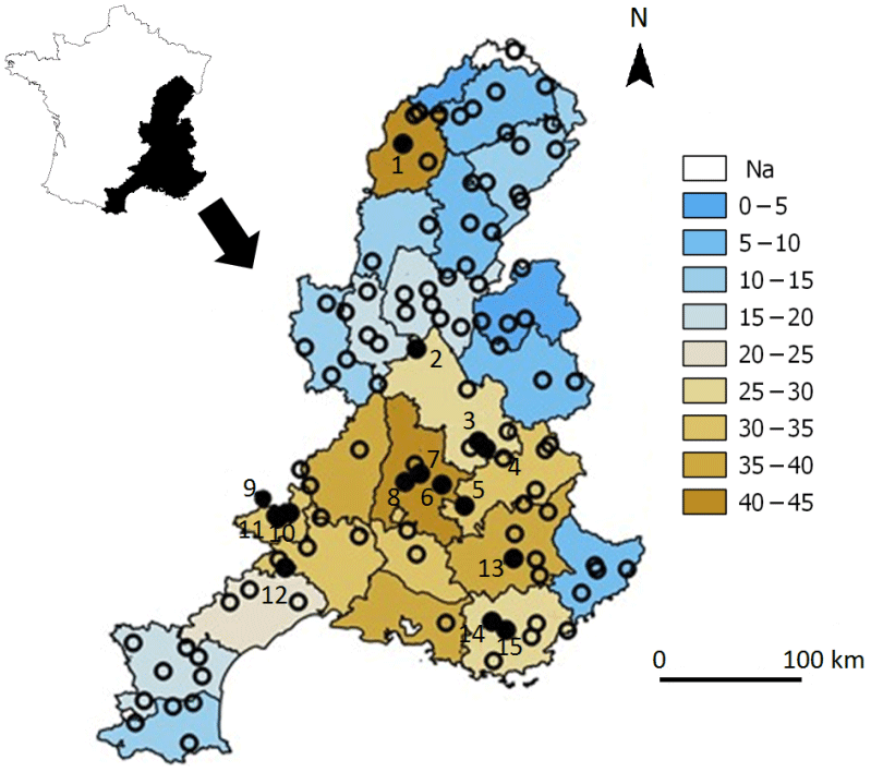
Figure 1The Rhône–Mediterranean water district, the total number of WR decisions stated by department over the period 2005–2016 and the gauged catchments (∘) where WR decisions are simulated (• denotes the subset of the 15 catchments used for evaluation purposes, and the figures are the related ranks presented in Table 1).
Water is globally abundant but uneven between the mountainous areas and the northern and southern parts of the RM district, and water resources are under high pressure due to water abstractions. For the period 2008–2013, annual total water withdrawal was around 6×10⁹ m3 (excluding any water abstraction for energy such as cooling nuclear plants and hydropower) with more used for irrigation (3.4×10⁹ m3, including 2×10⁹ m3 for channel conveyance). Use for public and industrial supply is 1.6×10⁹ and 1×10⁹ m3, respectively. Because of an intense competition for water between different users – agricultural, municipal and industrial – and the environment, some areas within the RM district can be vulnerable during low-flow periods. Around 40 % of the RM district suffers from water stress and scarcity (http://www.rhone-mediterranee.eaufrance.fr/gestion/gestion-quanti/problematique.php, last access: 1 August 2019) and has been identified by the French RM Water Agency as areas with persistent imbalance between water supply and water demand.
2.2 Drought management plan
DMPs define specific actions to be undertaken to enhance preparedness and increase resilience to drought. In France DMPs include regulatory frameworks to be applied in case of drought, called arrêtés cadres sécheresse. The past and operating DMPs and the water-restriction orders were inspected in the 28 departments of the RM district. They were obtained from the following:
-
the database of the DREAL Auvergne-Rhône-Alpes (“Direction Régionale de l'Eau, de l'Alimentation et du Logement” in French), including water-restriction levels (WRLs) and duration at the catchment scale available over the period 2005–2016 within the RM district,
-
the online national database PROPLUVIA (http://propluvia.developpement-durable.gouv.fr, last access: 1 August 2019), with WRLs and dates of adoption at the catchment scale for the whole of France available from 2012.
The most recent consulted documents date from January 2017.
2.3 Hydrological data
The hydrological observation dataset is a subset of the 632 French near-natural catchments identified by Caillouet et al. (2017). Daily flow data from 1958 to 2013 were extracted from the French HYDRO database (http://hydro.eaufrance.fr/, last access: 1 August 2019). Time series with more than 30 % missing values or more than 30 % null values were disregarded. Finally, the total dataset consists of 106 gauged catchments located in the RM district, with minor human influence and with high-quality data. The selected catchments are benchmark catchments where near-natural drought events are observed and current water availability is monitored. Water can be abstracted from other nearby streams.
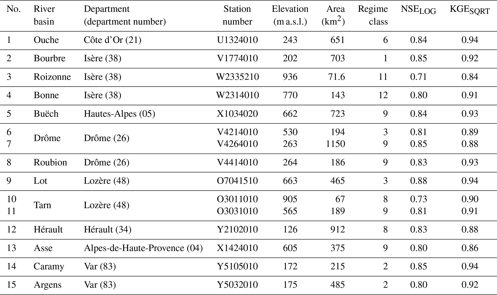
A selection of 15 evaluation catchments (Table 1) were used to calibrate and to evaluate the WRL (WR level) modelling framework (Sect. 4), selected because (i) they have complete records of stated water restriction, including dates and levels of restrictions – which was not the case in other catchments – and (ii) they are located in areas where water-restriction decisions are frequent. To facilitate interpretation, the 15 catchments were ordered along the north–south gradient. The Ouche and Argens river basins (no. 1 and 15 in Table 1) are the northernmost and the southernmost gauged basins, respectively. The 15 catchments encompass a large variety of river flow regimes according to the classification suggested by Sauquet et al. (2008; see Appendix A) that can be observed in the RM district (e.g. the Ouche – 1 in Table 1, pluvial regime; Roizonne – 3, transition regime; and Argens – 15, snowmelt-fed regime – river basins).
Table 1Main characteristics of the 15 catchments used for validation of water-restriction simulations. Station number refers to the catchment number in the HYDRO database, and regime class refers to the classification suggested by Sauquet et al. (2008) with a gradient from Class 1 – pluvial-fed regime –F moderately contrasting with Class 12 – snowmelt-fed regime.
2.4 Climate data
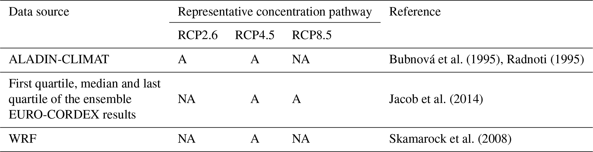
Baseline climate data were obtained from the French near-surface Safran meteorological reanalysis (Quintana-Seguí et al., 2008; Vidal et al., 2010) onto an 8 km resolution grid from 1 August 1958 to 2013. Exposure data were based on the regional projections for France (Table 2) available from the DRIAS French portal (http://www.drias-climat.fr/, last access: 1 August 2019, Lémond et al., 2011). Catchment-scale data were computed as a weighted mean for temperature and the sum for precipitation based on the river network described by Sauquet (2006).
Table 2Regional climate projections available in the DRIAS portal (A: available; NA: not available).
The “French Water Act” amended on 24 September 1992 (decree no. 92/1041) defines the operating procedures for the implementation of a DMP. Following the 2003 European heat wave, drought management plans including water restrictions have been gradually implemented in France (MEDDE, 2004). Water restrictions fall within the responsibility of the prefecture (one per administrative unit or department), as mentioned in article L211-3 II-1 of the French environmental code. Their role in drought management is to ensure that regulatory approvals for water abstraction continuously meet the balance between water resource availability and water uses including needs for aquatic ecosystems. De facto, legally binding water restrictions have to fulfil three principles: (i) being gradually implemented at the catchment scale with regards to low-flow severity observed at various reference locations, (ii) ensuring user equity and upstream–downstream solidarity, and (iii) being time-limited to fix cyclical deficits rather than structural deficits. The prefecture is in charge of establishing and monitoring the DMP operating in the related department.
Past and current drought management plans were analysed to identify the past and current modalities of application, the frequency of water-restriction orders, and the areas affected by water restrictions. Gathering and studying the regulatory documents was tedious in particular because of their lack of a clear definition of the hydrological variables used in the decision-making process.
This analysis shows that the implementation of the DMPs has evolved for many departments since 2003, e.g. with changes in the terminology and a national-scale effort to standardize WRLs. Now severity in low flows is classified into four levels, which are related to incentive or legally binding water restrictions. These measures affect recreational uses; vehicle washing; lawn watering; and domestic, irrigation and industrial uses (Table 3). Level 0 (called “vigilance”) refers to incentive measures, such as an awareness campaign to promote low water consumption from public bodies and the general public. Levels 1 to 3 are incrementally legally binding restriction levels; level 1 (called “alert”) and 2 (called “reinforced alert”) enforce reductions in water abstraction for agriculture uses or several days a week of suspension. Level 3 (called “crisis”) involves a total suspension of water abstraction for non-priority uses, including abstraction for agricultural uses and home gardening, and authorizes only water abstraction for drinking water and sanitation services. Due to change in the naming of WRLs since their creation, one task was dedicated to restate the WR decisions (hereafter “OBS”) since 2005 with respect to the current classification into four WRLs.
Table 3Uses affected by water restriction according to the drought severity.

For all catchments, a WR decision chronology was derived, showing a large spatial variability in WR (Fig. 1); note that the 15 evaluation catchments (Table 1) are located in the most affected areas. Between 2005 and 2012, WR decisions were mainly adopted between April and October (98 % of the WR decisions; Fig. 2), with 62 % in July or August, peaking in July.
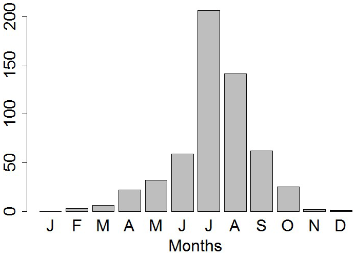
Figure 2Total number of stated WR decisions over the RM district per month over the period 2005–2016.
Decisions for adopting, revoking or upgrading a WR measure are taken after consultation of “drought committees” bringing the main local stakeholders together, the meeting frequency of which is irregular and depends on hydrological drought development. The adopted restriction level is mainly based on the existing hydrological conditions at the time, i.e. based on low-flow monitoring indicators measured at a set of reference gauging stations and their departure from a set of regulatory thresholds. This varies greatly across the RM district (Fig. 3). The low-flow monitoring indicators usually considered are as follows:
-
the daily discharge Qdaily,
-
the maximum discharge for a window with length d days, , , and
-
the mean discharge for a window with length d days, .
Both and are computed over the whole discharge time series on moving time windows with duration d, associated with the WR decision varying between 2 and 10 d depending on DMPs. (40 % of DMPs) and (17 % of DMPs) are the most commonly used, but other single indicators include Qdaily (17 %), (14 %), (8 %), (3 %) and (3 %), with mixed indicators also being used (e.g. 14 % of and Qdaily together).
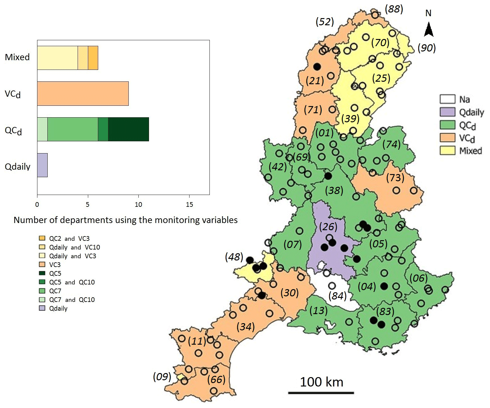
Figure 3Low-flow monitoring variables used in the current drought management plans. Qdaily denotes daily streamflow, denotes the d-day maximum discharge, refers to the d-day mean discharge, and “Mixed” refers to combinations of the aforementioned variables. Department codes are given in brackets.
The threshold associated with WR also varies within the district, generally associated with statistics derived from low-flow frequency analysis but also fixed to locally defined ecological requirements. In the context of DMPs, series of minimum or values are calculated by the block minimum approach and thereafter fitted to a statistical distribution. The block is not the year but the month, or it is given by the division of the year into thirty-seven 10 d time windows. The regulatory thresholds are given by quantiles with four different recurrence intervals associated to the four restriction levels. Generally, return periods T of 2, 5, 10 and 20 years are associated with the vigilance, alert, reinforced alert and crisis restriction levels, respectively. For example, let us consider thresholds based on the annual monthly minima of . The block minimum approach is carried out on the N years of records for each month i, i=1 …, 12, leading to 12 datasets, {min, month(t)=i, year(t)=j}, j=1, …, N}. The 12 fitted distribution allows the calculation of 48 values of thresholds (month-VCNd; 12 months × 4 levels) with four T-year recurrence intervals.
The meteorological situation is also examined in terms of precipitation deficit and likelihood of significant rainfall event considering available short- to medium-range weather forecasts. There are heterogeneities in the drought-monitoring variables, the time period on which deficit is calculated and the permissible deviation from long-term average values.
Where appropriate, other supporting local observations such as groundwater levels, reservoir water levels, field surveys provided by the ONDE network (Beaufort et al., 2018) or feedbacks from stakeholders can be used to inform final decisions.
Since their creation, DMPs have been frequently updated regarding the definition of the regulatory thresholds and the monitoring variables, the water uses affected by legally binding restrictions, the selection of the monitoring sites, etc. It was especially done following the publication of the report of the French ministry of Ecology in May 2011, and updates often occur after a year with a severe drought to include feedbacks and lessons for the future. Decision-making processes are definitely heterogeneous in both time and space, which does not make the WR modelling easy. In addition, official reports stated that the DMPs were not all available for this study. Facing this complexity, simplifying assumptions will be considered in the modelling framework presented in Sect. 4.3.4 (Risk-based framework and the related tools).
4.1 The scenario-neutral concept
Traditionally, hydrological impact studies are often based on “top-down” (scenario-driven) approaches and easy to interpret, but with associated conclusions becoming outdated as new climate projections are produced. In addition scenario-based studies may fail to match decision-making needs, since the implication in terms of water management is usually ignored (Mastrandrea et al., 2010). As a substitute to the scenario-driven approach, the scenario-neutral approach (Brekke et al., 2009; Prudhomme et al., 2010, 2013a, b, 2015; Brown et al., 2012; Brown and Wilby, 2012; Culley et al., 2016; Danner et al., 2017) has been developed to better address risk-based decision issues. The suggested framework shifts the focus to the current vulnerability of the system affected by changes and to critical thresholds above which the system starts to fail to identify possible maladaptation strategies (Broderick et al., 2019). Applied to water management issues, the scenario-neutral studies (Weiß, 2011; Wetterhall et al., 2011; Brown et al., 2011; Whateley et al., 2014) aim at improving the knowledge of the system's vulnerability to changes and at bridging the gap between scientists and stakeholders facing needs in relevant adaptation strategy. Prudhomme et al. (2010) have suggested combining of the sensitivity framework with top-down projections through climate response surfaces. This approach has been applied to low flows in the UK (Prudhomme et al., 2015), and its interests have been discussed as a support tool for drought management decisions.
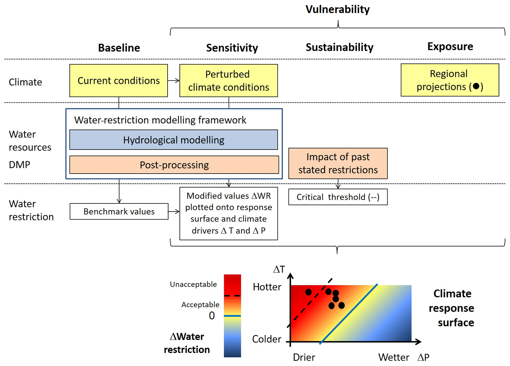
Figure 4Schematic framework of the developed approach to assess the vulnerability of the DMPs under climate change.
The risk-based framework adopted contains three independent components (Fig. 4):
- i.
Sensitivity analysis (Fronzek et al., 2010) is based on simulations under a large spectrum of perturbed climates to (a) quantify how policy-relevant variables respond to changes in different climate factors and (b) identify the climate factors that the system is the most sensitive to. Addressing (a) and (b) may help modellers in checking the relevance of their model (e.g. unexpected sensitivity to a climate factor regarding the known processes influencing the rainfall–runoff transformation). From an operational viewpoint, it may encourage stakeholders to monitor, with priority, the variables that affect the system of interest (reinforcement of the observation network, literature monitoring, etc.).
- ii.
Sustainability or performance assessment aims to identify under which climate (or other) conditions (e.g. no-rain period in spring, heat wave in summer, etc.) the system fails. A key challenge in the bottom-up framework is to define performance metrics and associated critical thresholds relevant to the system of interest. In the case of our study, these thresholds will make it possible to distinguish the duration of water restrictions which is unacceptable for users.
- iii.
Exposure is defined by state-of-the-art regional climate trajectories superimposed to the climate response surface. The exposure measures the probability of changes occurring for different lead times based on available regional projections.
All the components of the framework together contribute to the vulnerability of the system (including its management) to systematic climatic deviations.
The sensitivity analysis was conducted by applying a water-restriction modelling framework. Climate conditions were generated by applying incremental changes to historical data (precipitation and temperature) and introduced as inputs in the developed models to derive occurrence and severity of water restriction under modified climates. The tool chosen here to display the interactions between water restriction and the parameters that reflect the climate changes is a two-dimensional response surface, with axes represented by the main climate drivers. This representation is commonly used in scenario-neutral approach. For example, in both Culley et al. (2016) and Brown et al. (2012), the two axes were defined by the changes in annual precipitation and temperature. When changes affect numerous attributes of the climate inputs, additional analyses (e.g. elasticity concept combined with regression analysis – Prudhomme et al., 2015; the Spearman rank correlation and Sobol sensitivity analyses – Guo et al., 2017) may be required to point out the key variables with the largest influence on water restriction that form thereafter the most appropriate axes for the response surfaces.
Performance assessment is a challenging task for hydrologists, since it requires information on the impact of extreme hydrometeorological past events on stakeholders' activities. Simonovic (2010) used observed past events selected with local authorities on a case study in southwestern Ontario (Canada), chosen for their past impact (flood peak associated with a top-up of the embankments of the main urban centre; level 2 drought conditions of the low water response plan). Schlef et al. (2018) set the threshold to the worst modelled event under current conditions. Whateley et al. (2014) assessed the robustness of a water supply system, and the threshold is fixed to the cumulative cost penalties due to water shortage evaluated under the current conditions. Brown et al. (2012) and Ghile et al. (2014) suggested selecting thresholds according to expert judgment of unsatisfactory performance of the system by stakeholders, whilst Ray and Brown (2015) use results from cost–benefit analyses. The spatial coverage of a large area, such as the RM district, and the heterogeneity in water use (domestic needs, hydropower, recreation, irrigation, etc.) make it challenging for a systematic, consistent and comparable stakeholder consultation to be conducted and for a relevant critical threshold Tc to be fixed for all the users. Facing this complexity, only the irrigation water use will been examined here, since it is the sector which consumes most water at the regional scale, with a critical threshold defined for this single water use.
Exposure to changes here is measured using regional projections, visualized graphically by positioning the regional projections in the coordinate system of the climate response surfaces and identifying the associated likelihood of failure relative to Tc. Note that, to update the risk assessment, only the exposure component has to be examined (including the latest climate projections available onto the response surfaces).
4.2 The rainfall–runoff modelling
The conceptual lumped rainfall–runoff model GR6J was adopted for simulating daily discharge at 106 selected catchments of the RM district. The GR6J model is a modified version of GR4J originally developed by Perrin et al. (2003), which is well suited to simulate low-flow conditions (Pushpalatha et al., 2011). The four-parameter version of the model GR4J has been progressively modified. Le Moine (2008) has suggested a new groundwater exchange function and a new routing store representing long-term memory in the GR5J model. Pushpalatha et al. (2011) finally introduced in the GR6J model an exponential store parallel to the existing store of the GR5J model. Considering additional routing stores is consistent regarding the natural complexity of hydrological processes, and in particular, the dynamics of flow components in low flows (Jakeman et al., 1990).
The GR6J model has six parameters to be fitted (Fig. 5): the capacity of soil moisture reservoir (X1) and of the routing reservoir (X3), the time base of a unit hydrograph (X4), two parameters of the groundwater exchange function F (X2 and X5), and a coefficient for emptying the exponential store (X6). The GR6J model is combined here with the CemaNeige semi-distributed snowmelt runoff component (Valéry et al., 2014). The catchment is divided into five altitudinal bands of equal area on which snowmelt and snow accumulation processes are represented. For each band, daily meteorological inputs – including solid fractions of precipitation – are extrapolated using elevation as a covariate, and the snow routine is calculated separately. Finally, its outputs are then aggregated at the catchment scale to feed GR6J. The two parameters of CemaNeige, S1 and S2, control the snowpack inertia and the snowmelt, respectively. S1 is used to compute the thermal state of the snowpack eTG, which is an equivalent to the internal snowpack temperature (∘C). eTG(t) at day t is a weighted linear combination of the value of eTG(t−1) (×S1) and the air temperature at the day t (). S2 is the snowmelt degree-day factor used to calculate the daily snowmelt depth by multiplying the air temperature when it exceeds 0 ∘C, with S2. The splitting coefficient (SC) of effective rainfall between the two stores (in Fig. 5) has been fixed to 0.4 by Pushpalatha et al. (2011), since calibrating the SC leads to only slightly better performance. The allocation of the outflow from the soil moisture reservoir, with 90 % being percolation and 10 % being surface and sub-surface runoff in the GR6J model, is the result of previous studies. The GR6J model was selected for its good performance across a large spectrum of river flow regimes (e.g. Hublart et al., 2016; Poncelet et al., 2017).
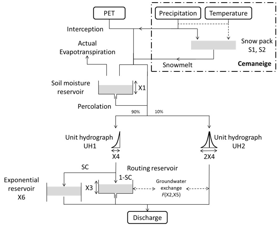
Figure 5Schematic of the rainfall–runoff model GR6J combined with the CemaNeige snowmelt runoff component (after Pushpalatha et al., 2011).
No routine to simulate water management (e.g. reservoir) was considered here, since discharges of the 106 gauging stations are weakly altered by human actions or naturalized discharges (i.e. flows corrected from the effects of water use). The eight parameters (six from the GR6J model and two from the CemaNeige module) were calibrated against the observed discharges using the baseline Safran reanalysis as input data and the Kling–Gupta efficiency criterion (Gupta et al., 2009) KGESQRT calculated on the square root of the daily discharges as an objective function. The KGESQRT criterion was used to place less emphasis on extreme flows (both low and high flows). As the climate sensitivity space includes unprecedented climate conditions (including colder climate conditions around the current-day condition), the CemaNeige module was run for all the 106 catchments, even for those not currently influenced by snow.
The two-step procedure suggested by Caillouet et al. (2017) was adopted for the calibration: first the eight free parameters were fitted only for the catchments significantly influenced by snowmelt processes – i.e. when the proportion of snowfall to total precipitation less than 10 % – and second, for the other catchments, the medians of the CemaNeige parameters were fixed, and the six remaining parameters were then calibrated. Calibration is carried out over the period 1 January 1973 to 30 September 2006, with a 3-year spin-up period to limit the influence of reservoir initialization on the calibration results. The criterion KGESQRT and the Nash–Sutcliffe efficiency criterion on the log-transformed discharge NSELOG (Nash and Sutcliffe, 1970) were calculated over the whole period 1958–2013 for the subset of 15 evaluation catchments (Table 1), showing KGESQRT and NSELOG values are above 0.80 and 0.70, respectively. These two goodness-of-fit statistics indicate that GR6J adequately reproduces observed river flow regime, from low- to high-flow conditions. The less satisfactory performances of GR6J are observed for the Tarn and Roizonne river basins, both characterized by smallest drainage areas and highest elevations of the dataset. These lowest performances are likely to be linked to their location in mountainous areas (snowmelt processes are difficult to reproduce) and to their size (the grid resolution of the baseline climatology fails to capture the climate variability in the headwaters).
4.3 The water-restriction-level modelling framework
The WRL modelling framework developed aims to identify periods when the hydrological monitoring indicator is consistent with legally binding water restrictions. Only physical components (mainly hydrological drought severity) leading to WR decisions are considered, with no sociopolitical factor accounted for to model water restrictions.
To enable comparison of results across all catchments – in particular to combine response surfaces obtained from different catchments (see Sect. 5.1) – the same drought-monitoring indicators and regulatory thresholds were adopted in all the catchments (see Sect. 3 for details), selected as the most commonly used in the 28 DMPs across the RM district, specifically choosing as a monitoring indicator and 10d-VCN3(T) with return periods T of 2, 5, 10 and 20 years as regulatory thresholds. Each regulatory threshold is defined for a 10 d calendar period between 1 April and 31 October, resulting in 21 sets of four thresholds. Water restrictions are decided after consulting drought committees that convene irregularly depending on hydrological conditions over a time window, i.e. the last N days. Here a time window for analysis of N=10 d was decided, which is consistent with the prefectural decision-making time frame (frequency of updates in water-restriction statements). The WRL modelling time step is finally fixed to 10 d, and a representative value of WRL is given to the twenty-one 10 d calendar periods from April to October. Thus WRL is thus computed as follows:
-
is computed from daily discharge Qdaily(t) every day t.
-
is compared to the corresponding regulatory thresholds to create time series of daily water-restriction level “wrl”, with wrl(t) ranging from 0 (no alert) to 3 (crisis):
-
If 10d-, wrl(t)=0.
-
If 10d-, wrl(t)=1.
-
If 10d-, wrl(t)=2.
-
If 10d-, wrl(t)=3.
-
-
A WRL(d) time series is created as the median of wrl(t) for each 10 d period.
-
The WRL(d) value is set to zero if preceding 10 d precipitation total exceeds 70 % of inter-annual precipitation average (precipitation correction).
Inputs of the WRL model are daily discharges and precipitation. Outputs are WRL time series with values for each twenty-one 10 d calendar period from April to October. Modelling is only applied to the period April–October, the irrigation period and when most water restrictions are put in place. The low-flow monitoring indicator and the regulatory thresholds 10d-VCN3(T) are computed from daily discharge time series Qdaily based on full period of records prior to 31 December 2013. The log-normal distribution is used to assess the return periods.
The WRL modelling framework can be applied to both observed and simulated time series. For the latter, outputs from GR6J are used for simulations under current and modified climate conditions. Regulatory thresholds are derived from simulated discharge using the Safran baseline meteorological reanalysis as input to moderate the possible effect of bias in rainfall–runoff modelling.
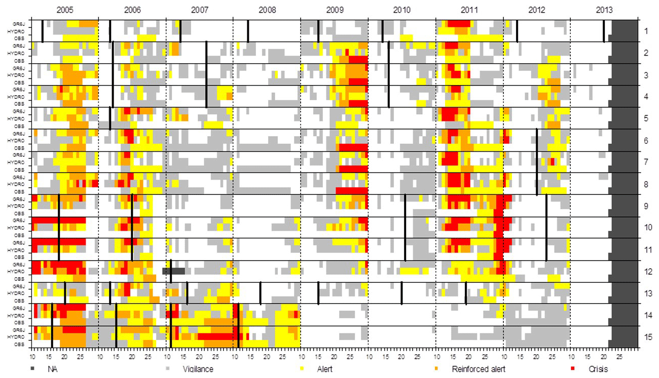
Figure 6Observed and simulated water-restriction levels considering the two sources of discharge data, GR6J and HYDRO, for each of the 15 evaluation catchments (Table 1). The x abscissa is divided into 10 d periods for each year, spanning the period April–October. Black segments identify updated DMPs.
The WRL modelling framework was verified in the 15 evaluation catchments (Table 1). WRL simulations based on modelled (hereafter GR6J) and observed (hereafter HYDRO) discharge were compared graphically to official WR measures (OBS). A further assessment was conducted using the Sensitivity and Specificity scores (Jolliffe and Stephenson, 2003) to examine how well the WRL modelling framework can discriminate WR severity levels (Table 4). The Sensitivity score assesses the probability of event detection; the Specificity score calculates the proportion of “no” events that are correctly identified. An event was defined as any legally binding water restriction of at least level 1, and a “non-event” was described as a period where WRL is zero or without WR. Comparisons were made over the 2005–2013 period, corresponding to the common period of availability for OBS, HYDRO and GR6J.
Table 4Contingency table for legally binding water restriction (WR*).

Figure 6 shows years with severe simulated WRLs (e.g. 2005 and 2011) and years with no or few simulated WRs (e.g. 2010 and 2013). Both GR6J and HYDRO simulations are generally consistent with OBS, even if misses are found (e.g. basins 9 to 11 during the year 2005). There is no systematic bias, with some overestimations (e.g. 2005 using GR6J in basins 1 and 15; 2007 using HYDRO in basin 15), underestimations (e.g. 2009 in basin 6–8) and misses (e.g. 2005 using HYDRO in basin 1).
Sensitivity and Specificity scores computed with OBS considered to be a benchmark (Fig. 7) show a large variation across the catchments, in particular for Sensitivity. Specificity scores are around 0.85 for both GR6J and HYDRO, suggesting that more than 85 % of the observed non-events were correctly simulated by the WRL modelling framework. The median of WRL Sensitivity score with HYDRO is around 45 %, indicating that for half the catchments, fewer than 45 % of observed events are detected based on HYDRO discharges, but this increases to 68 % of events detected when WRLs are simulated based on GR6J discharge. Using GR6J is more effective for detecting legally binding restriction than using observed discharges, while it is less efficient for predicting periods without restriction for most of the catchments. There is a compensatory effect, which is not easy to detect graphically, since Sensitivity scores are more sensitive than Specificity scores due to the reduced number of observed days with adopted restrictions. No evidence of systematic bias associated with catchment location or river flow regime was found: northern (blue) and southern (red) catchments are uniformly distributed in the Sensitivity and Specificity space.
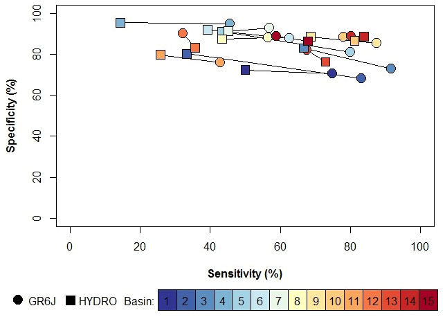
Figure 7Skill scores obtained for the WRL model over the period 2005–2013. Each segment is related to one of the 15 catchments listed in Table 2. The endpoints refer to the source of discharge data (GR6J or HYDRO).
Sensitivity and Specificity scores using HYDRO as a benchmark in the contingency table were also used to compare simulations from GR6J discharge with those obtained from HYDRO discharge. Median values reach 84 % (Sensitivity) and 92 % (Specificity), showing high consistency between HYDRO and GR6J. No statistical link between the hydrological model and WRL model performance was found, with R2 between NSELOG and Sensitivity or NSELOG and Specificity lower than 7 %. In addition, the similar skill scores of GR6J and HYDRO modelling suggest that possible biases in rainfall–runoff modelling does not impact on the ability of the WRL modelling framework to correctly simulate declared or undeclared WRs.
Choosing the same definitions for the monitoring indicator and regulatory thresholds is a simplifying assumption and may partly explain the deviations between simulated (HYDRO or GR6J) and adopted (HYDRO) WR measures. Before stating for and 10d-VCN3 the four prevalent modalities found in the current DMPs have been tested to reproduce the observed WR, and results have shown weak variables considered in the WR modelling framework. The mains reasons are that all the indicators and thresholds are derived from Qdaily time series and are highly correlated and thus share, above all, the same information on the dynamics and on the severity of drought.
Heterogeneity in basin characteristics and rules imposed by the DMPs should not result in a systematic difference in the Sensitivity and Specificity score between GR6J and HYDRO identified for most of the 15 evaluation catchments. Simulations were made on near-pristine catchments, and thus water uses are unlikely to be the main reason. Other causes of higher Sensitivity scores obtained when simulated discharges are used as input have been investigated in the WRL modelling framework. However, results of this analysis have not been conclusive. The aforementioned tests with the four prevalent modalities have all led to a higher Sensitivity score using GR6J and a higher Specificity score using HYDRO, demonstrating that the choice of the monitoring indicator and regulatory thresholds is probably not involved. A “smoothing” introduced by the hydrological modelling was also suspected, but autocorrelation in observed and GR6J-simulated time series was found to be very similar. Future works may reinvestigate these aspects. They will need to explore new aspects (e.g. the way WRL is derived from the daily values wrl for each 10 d period) using a longer verification period with a not necessarily uniform but fixed regulatory framework. Indeed some catchments have experienced only 3 years with legally binding water restrictions and DMPs were frequent during the 2005–2013 period (see the black vertical segments in Fig. 6).
Discrepancy between simulated and adopted WR measures is most likely due to the other factors involved in the decision-making process. When regulatory thresholds are crossed, restrictive measures should follow the DMPs. In reality, the measures are not automatically imposed but are the result of a negotiating process. This process includes for example some expert-judgment factors such as (i) the evolution of low-flow monitoring indicators and thresholds over the years – e.g. annual revision for the Ouche and irregular revision for the Isère (38), Gard (30), Alpes-de-Haute-Provence (04) and Lozère (48) departments (last one in 2012); (ii) the role of drought committees in negotiating a delay in WRL applications to limit economic damages or to harmonize responses across different administrative sectors sharing the same water intake; and (iii) the local expertise, especially regarding the uncertainty in flow measurements (Barbier et al., 2007) impacting the low-flow monitoring indicators, e.g. Côte d'Or (21) and Lozère (48) in the northern and southwestern parts of the RM district, respectively. Note that where WR decisions are not uniquely based on hydrological indicators but also involve a negotiation process, the results of the WRL modelling framework should be interpreted as potential hydrological conditions for stating water restrictions.
Results of our sample study on 15 evaluation catchments show deviations for most catchments but links between order restrictions and hydrological drought severity. These deviations may partly be attributed to the use of the same monitoring indicator and regulatory thresholds across the catchments in the modelling (whilst it is not true in reality) as a necessary assumption for a regional-scale analysis. Tests with as low-flow monitoring variable combined with the two dominant modalities for the regulatory thresholds show a weak sensitivity of the WRL modelling skill to the choice of the indicators (with a slight increase in Specificity score – ∼90 % – while the Sensitivity score is reduced – <50 % – using GR6J). Whilst the developed WRL modelling framework does not account for the expert decision made by drought committees – and hence is not designed to simulate the exact WR decisions – its ability to simulate 68 % of the stated restrictions over the period 2005–2013 demonstrates its usefulness as a tool to objectively simulate the potential of drought restrictions based on hydrological drought physical processes. The methodology was applied to the 106 catchments of the RM district under climate perturbations to assess the potential impact of climate change on water restriction in the region. The resulting analysis focuses on water-restriction level higher than 1, denoted thereafter as WR*.
4.4 The generation of perturbed climate conditions
The generation of climate response surfaces relies on synthetic climate time series representative of each explore climate condition and used as input to the impact modelling chain (here hydrological model and WRL modelling framework). Methods based on stochastic weather simulation have been used (Steinschneider and Brown, 2013; Cipriani et al., 2014; Guo et al., 2016, 2017), but it can be complex to apply them in a region with such a heterogeneous climate as the RM district. Alternatively, the simple “delta-change” method (Arnell, 2003) has been commonly used to provide a set of perturbed climates in a scenario-neutral approach (Paton et al., 2013; Singh et al., 2014) and was used here, similar to Prudhomme et al. (2010, 2013a, b, 2015).
Following Prudhomme et al. (2015), monthly correction factors ΔP and ΔT are calculated using single-phase harmonic functions:
with P0 and T0 as mean annual changes in precipitation (Eq. 1) and temperature (Eq. 2), respectively, i as the indicator of the month (from 1 to 12), φ as the phase parameter, and A as the semi-amplitude of change (e.g. half the difference between highest and lowest values) for precipitation (Eq. 1) and temperature (Eq. 2). These correction factors were applied to the baseline climate datasets to create perturbed daily forcings:
with P(d) and T(d) representing baseline precipitation and temperature values for day d, P*(d) and T*(d) representing the corrected (or perturbed) values for day d, and representing average monthly baseline precipitation for month(d). Corrected potential evapotranspiration PET* time series were derived from temperature values using the formula suggested by Oudin et al. (2005):
with PET(d) as baseline potential evapotranspiration values for day d; Ra is the extraterrestrial global radiation for the catchment.
The baseline climate (precipitation and temperature) time series were extracted from the Safran reanalysis over the period 1958–2013 (56 years), and perturbed time series were generated for the same length. The range of climate change factors to generate the perturbed series were chosen to encompass both the range and the seasonality of RCM-based (RCM – regional climate model) changes in projections in France. A set of 45 precipitation and 30 temperature scenarios was created (Fig. 8), spanning the range of potential future climate suggested by Terray and Boé (2013) and combined independently, resulting in a total of 1350 precipitation and temperature perturbations pairs used to define the climate sensitivity space. In this application, the following applies:
-
P0 (mm) = , j=1, …, 9,
-
AP (mm) = , j=1, …, 5,
-
T (∘C) = j−1, j= 1, …, 6,
-
AT (∘C) = , j=1, …, 5,
-
φP parameter is fixed to 1 to consider minimum change in January and maximum change in July, and
-
φT is fixed to 2 to get maximum change in August.
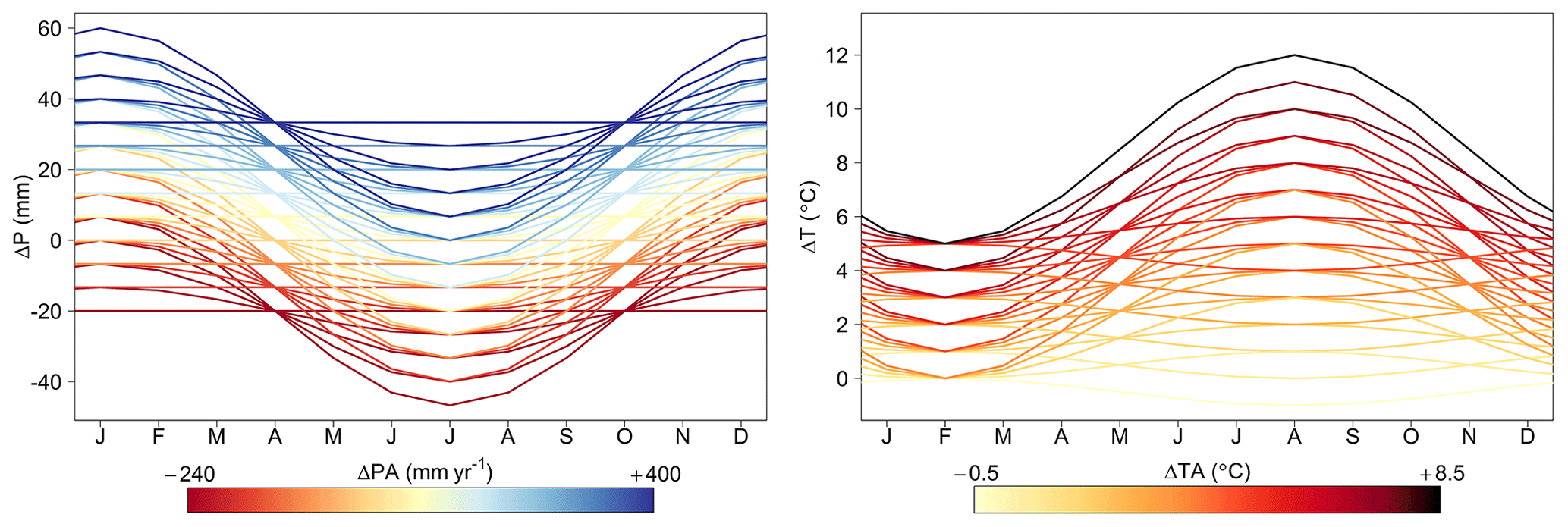
Figure 8Monthly perturbation factors ΔP and ΔT associated with the climate sensitivity domain. The colour of the line is related to the intensity of the annual change ΔPA and ΔTA.
4.5 The assumptions on water uses
Water uses and the feedbacks between use and available resources are not explicitly addressed in this application either under current or future conditions. This should not be considered to be a limitation for basins where hydrological modelling has been implemented. Indeed, the 106 basins under study have been carefully chosen, since they are currently influenced little or are not influenced by human actions. These catchments are benchmark catchments where natural water availability is monitored for the statement of restriction orders. Water can be abstracted from other neighbouring rivers. Water needs will probably evolve in the coming decades. The water requirement for irrigation may increase parallel to air temperature or may decrease due to adaptive actions (e.g. farmers may choose to plant specific crops less sensitive to water shortages). Water needs and sensitivity to water restrictions depend on socio-economic and institutional pathways. Forward-looking studies have been recently carried out with the involvement of local experts but at the local scale (Grouillet et al., 2015 for the Hérault river basin; Andrews and Sauquet, 2017 for the Durance river basin). The distinct underlying assumptions make it difficult to combine and to extend the prospective scenarios over the RM district. Thus, the water-restriction modelling framework considers, in this application, the “business-as-usual” scenario, which assumes that only minor change in water demand behaviour will occur. In particular, no major alteration of the river flow regime is projected for the 106 catchments. Despite being unrealistic, maintaining the current conditions allows for the assessment of the impact of climate change regardless of any other human-induced changes. The advantage is that results are easier to understand and to embrace by stakeholders than those obtained with complex multi-sectorial scenarios that they may not identify with.
5.1 The water-restriction response surfaces
The 1350 sets of perturbed precipitation, temperature and PET time series were each fed into the WRL modelling framework for each of the 106 catchments. Both (monitoring indicators) and 10d-VCN3(T) (regulatory thresholds) were computed from GR6J 56-year discharge simulations. For each scenario, the number of 10 d periods under a water restriction of at least level 1 (WR*) was calculated and expressed as a deviation from the simulated baseline value, ΔWR*, hence removing the effect of any systematic bias from the WRL modelling framework. Results are shown as WR response surfaces built with x and y axes that represent key climate drivers. Because different climate perturbation combinations share the same values of the key climate drivers, hence being represented at the same location of the response surface, the median ΔWR* from all relevant combinations is displayed as a colour gradient, with the standard deviation (SD) of ΔWR* shown as the size of the symbol.
Response surfaces based on different climate variables for x (precipitation) and y (temperature) were generated over the whole or part of the water-restriction period (April to October – AMJJASO; March to June – MAMJ; and July to October – JASO, the latter coinciding with the highest temperatures) and visually inspected to identify the greatest signal pattern, combined with the smallest dispersion around the surface response (i.e. analysis of the median and the maximum of SD values over the grid cells).
The response surfaces are exemplified on three of the 15 evaluation catchments (Table 1, Fig. 9):
-
the Argens river basin, along the Mediterranean coast, where severe low flows occur in summer and actual evapotranspiration is limited by water availability in the soil;
-
the Ouche river basin, in the northern part of the RM district, a typical pluvial river flow regime under oceanic climate influences where runoff generation is less bounded by evapotranspiration processes;
-
the Roizonne river basin, in the Alps, typical of summer flow regime controlled by snowmelt, with spring to summer climate conditions dominating changes in low flows.
The visual inspection of response surfaces shows the following:
-
ΔWR* is differently driven by the changes in precipitation ΔP and in temperature ΔT: ΔWR* is very sensitive to ΔP in the Argens river basin (horizontal stratification in the response surface) and to ΔT in the Roizonne river basin (vertical stratification in the response surface) whilst being controlled by both drivers in the Ouche river basin.
-
There is a high likelihood of an increase in the duration of water restriction in the Roizonne river basin, as shown by a response surface dominated by positive ΔWR*.
-
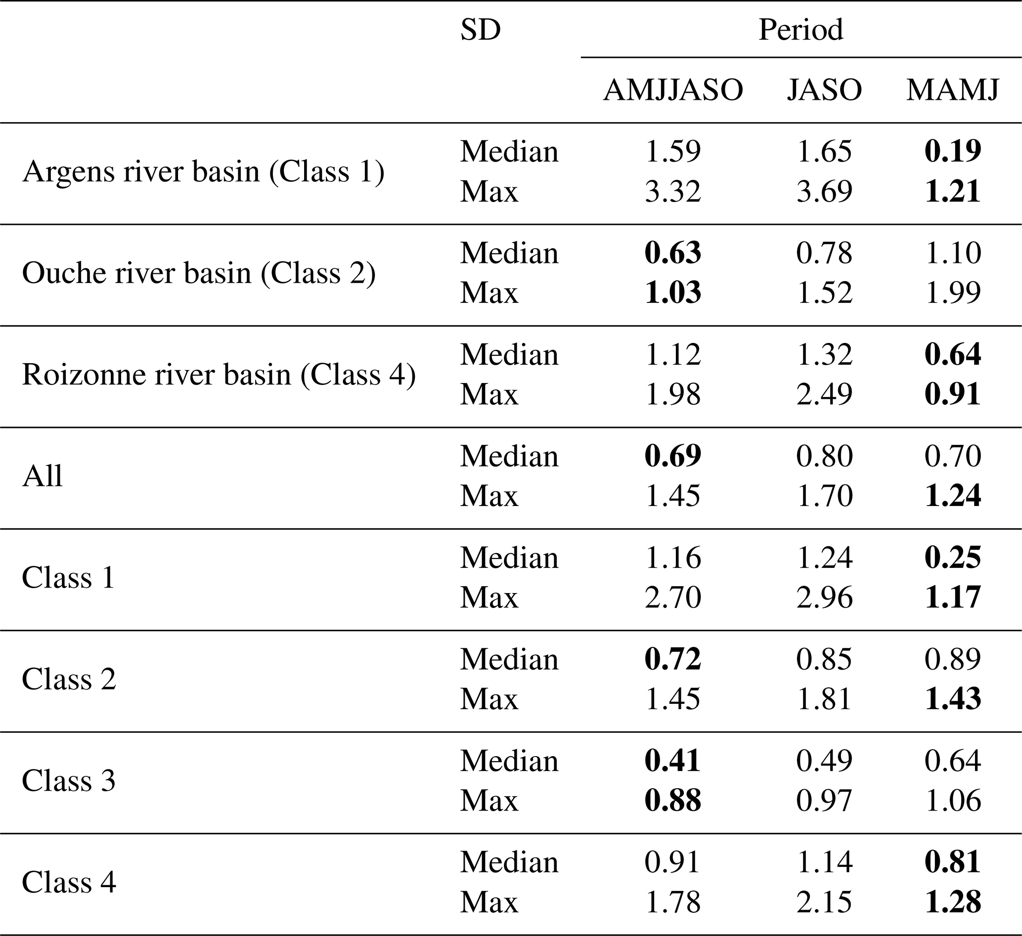
SD values may vary significantly from one graph to another (Table 5). For both the Argens and Roizonne river basins, the largest SDs are found when the response surfaces are displayed with climate variables computed over the whole period April–October (AMJJASO), while smallest SDs are associated with ΔP and ΔT drivers from March to June. Changes in mean spring to early summer precipitation and temperature mainly govern changes in WR* for these two basins. Conversely changes in precipitation ΔP and temperature ΔT over the full period April–October seem to be the dominant drivers of changes in WR* for the Ouche river basin.
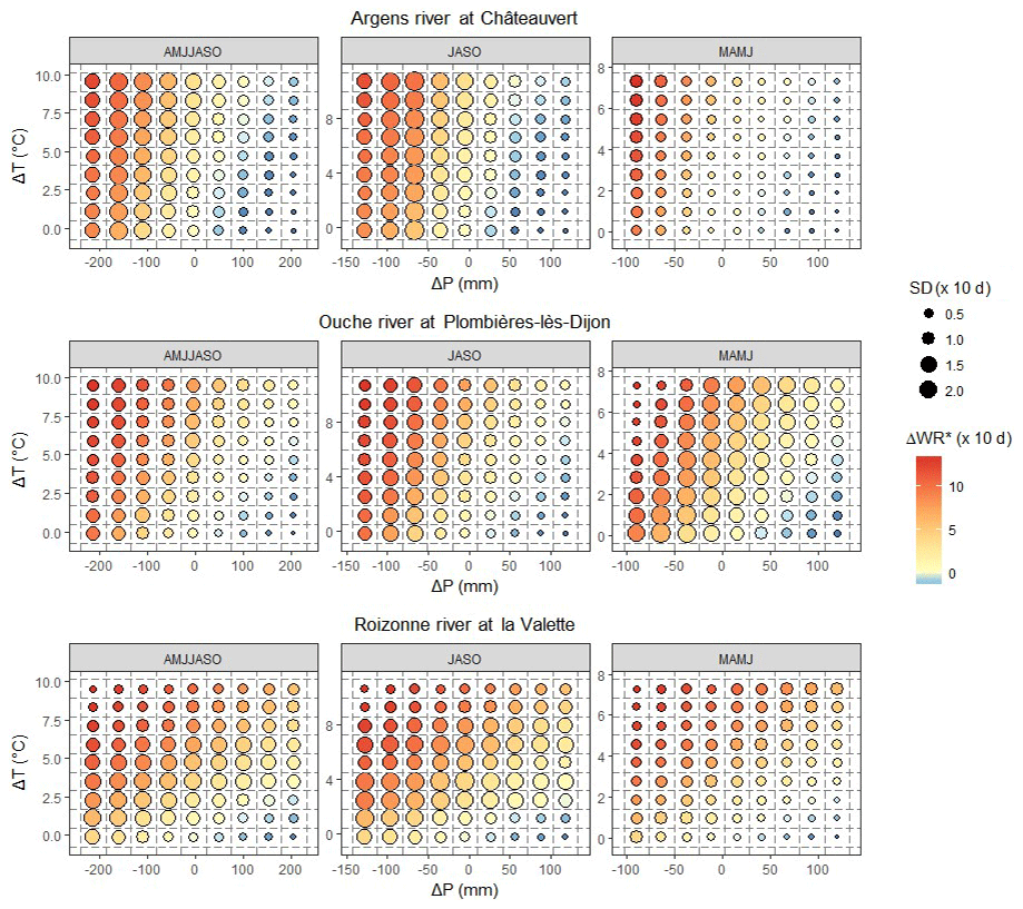
Figure 9Climate response surface of legally binding water-restriction-level anomalies ΔWR* for the Argens, Ouche and Roizonne river basins. Each graph is obtained considering changes in mean precipitation ΔP and temperature ΔT over a specific period as x and y axis.
Table 5Summary statistics for standard deviation (SD) of the grid for different axes. Best results are in bold characters.
5.2 Response surface analysis at the regional scale
Following Köplin et al. (2012) and Prudhomme et al. (2013a), the 106 response surfaces were classified to define typical response surfaces, designed as tools to help in prioritizing actions for adapting water management rules to future climate conditions in the RM district. Here a hierarchical clustering based on Ward's minimum variance method and Euclidian distance as similarity criteria (Ward Jr., 1963) was applied, and four classes were identified after inspection of the agglomeration schedule and silhouette plots (Rousseeuw, 1987). A manual reclassification was conducted for the few catchments with negative individual silhouette coefficients to ensure higher intra-class homogeneity. For each class, a mean response surface and associated SD were computed, and main climate drivers associated with WR changes were identified (Table 5).
All suggest an increase in the occurrence of legally binding water restrictions when precipitation decreases or when temperature increases (Fig. 10). An additional temperature increase and its associated PET increase can compensate for precipitation increase and lead to a decrease in ΔWR*, with intra-class differences emerging in the magnitude of changes. The identified four typical water restriction response surfaces show a weak regional pattern and common features. Class 4 (including the Roizonne river basin) regroups snowmelt-fed river flow regimes in the Alps, whilst basins of Class 1 are mainly Mediterranean river flow regimes. Class 2 (including the Ouche river basin) and Class 3 catchments are partly influenced by both precipitation and temperature, with ΔWR* in Class 2 catchments being less sensitive to climatic changes (flatter WR response surface) than catchments of Class 3. The flow regime of Class 2 to 3 ranges from rainfall-fed regimes with high flow in winter and low flow in summer in the northern part of the RM district to regimes partly influenced by snowmelt, with high flows in spring in the Alps and in the Cevennes.

Figure 10Results of the hierarchical cluster analysis applied to the climate response surface WR*-level anomalies ΔWR*.
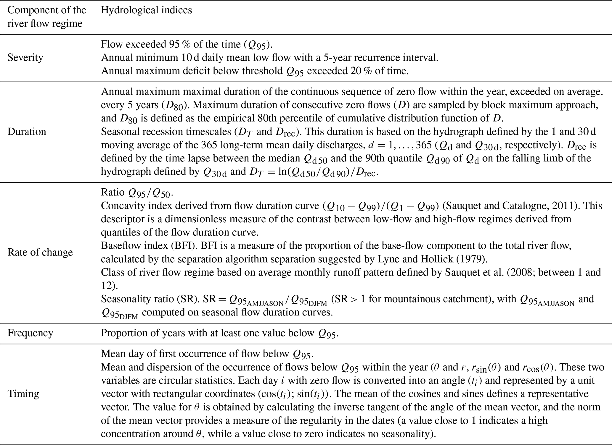
To further the regional analysis and help sensitivity assessment at unmodelled catchments, basin descriptors were investigated as possible discriminators of the four classes. A set of potential discriminators – which included measures of the severity, frequency, duration, timing and rate of change in low-flow events (Table 6); the drainage area and the median elevation for the catchment; and one climate descriptor (mean annual precipitation and mean annual potential evapotranspiration used to compute an aridity index – AI) – were introduced in a CART model (Classification And Regression Trees; Breiman et al., 1984), aimed at performing successive binary splits of a given dataset according to decision variables. Through a set of “if–then” logical conditions the algorithm automatically identifies the best possible predictors of group membership, starting from the most discriminating decision variable to the less important factors. The optimal choices are fixed recursively by increasing the homogeneity within the two resulting clusters. At each step, one of the clusters (node) is divided into two non-overlapping parts. Here, to free results from catchment size influence, descriptors related to severity were expressed in millimetres per year, millimetres per month or millimetres per day.
Table 6Hydrological metrics considered to investigate similarity in CART.
Results show three top discriminators, with the aridity index being the strongest:
-
the AI given by the mean annual precipitation divided by the mean annual potential evapotranspiration (UNEP, 1993),
-
the base-flow index (BFI), a measure of the proportion of the base-flow component to the total river flow, calculated by the separation algorithm separation suggested by Lyne and Hollick (1979),
-
the concavity index (CI; Sauquet and Catalogne, 2011) to characterize the contrast between low-flow and high-flow regimes derived from quantiles of the flow duration curve.
CART overall misclassification (18 %) suggests a satisfactory performance in the classification method, characterized by a parsimonious algorithm (five nodes and three variables) with the potential for a first-guess assessment of the WR response to disruptions and evaluation of the robustness of existing water restriction at the department-level scale. For each class, Fig. 11 shows the empirical distribution of the three main discriminators, the mean timing θ of daily discharge below Q95 and its dispersion r, which is based on circular statistics, where Q95 is the 95th quantile derived from the flow duration curve.

Figure 11Statistical distribution of the discriminating factors identified by the CART algorithm (a–c) and the mean timing θ of daily discharge below Q95 and its dispersion r (d). The boxplots are defined by the first quartile, the median and the third quartile. The whiskers extend to 1.5 of the interquartile range; open circles indicate outliers. The colour is associated to the membership to one class, and the name of the class is given along the x axis. The coloured areas in (d) are defined by the first quartile and the third quartile of r and θ. Each dot is related to one gauged basin. The dotted lines indicate the start of four meteorological seasons.
The classification discriminates catchments primarily on the seasonality of low-flow conditions and the aridity index, with the extreme classes (1 and 4) being particularly well discriminated.
Geographically, Class 1 catchments are mainly located along the Mediterranean coast and include the Argens river basin; ΔWR* is mainly driven by changes in precipitation in spring and early summer. Class 1 gathers water-limited basins with small values of the AI and a weak sensitivity to climate change in summer. In these dry water-limited basins, the mid-year period exhibits the minimal ratio P / PET, and changes in summer precipitation have hence only a moderate impact on low flows; spring is the only season when PET changes are likely to result in both actual evapotranspiration and discharge changes. WRLs are more likely controlled by antecedent soil moisture conditions in spring and early summer. This behaviour is typical of the basins under Mediterranean conditions and was discussed in the context of a scenario-neutral study in Australia (Guo et al., 2016). For those catchments, climate drivers computed in spring (over the period MAMJ) are used to describe the x and y axes of the response surface, fully consistent with water-limited basin processes.
Catchments of both Class 2 and 3 have a similar CI, hence suggesting that flow variability is not a proxy for low-flow response to climatic deviation. However, BFI values for Class 3 are lower than for Class 2, while Class 3 is characterized by high values for the AI. Despite higher capability to sustain low flows (see BFI values) the response surface representative of Class 2 is more contrasted than that of Class 3; a possible reason could be drier conditions under current conditions (the median of the AI equals 2.5 for Class 3 compared to 1.6 for Class 2). The monthly perturbation factors (see Sect. 5.1) are the same for all the classes, but the changes in relative terms are less significant regarding the current climate conditions for Class 3 than for Class 2 and may explain the limited changes in river flow patterns.
Class 4 regroups catchments with low flows in winter and significant snow storage. The BFI values are high, and due to smooth flow duration curves, the CI demonstrates also high values.
5.3 Risk assessment at the basin scale
The risk-based framework has been applied to the irrigation water use, since annual net total water withdrawal for agriculture purposes is ranked first at the regional scale. Note that in the Rhône–Mediterranean district around 90 % and 10 % of water used for irrigation originates from surface water and groundwater, respectively. To complement water needs irrigators may also have access to small reservoirs (storage capacity usually less than 1×10⁶ m3). Most of the reservoirs are filled by surface water in winter and release water later in the following summer. Water restrictions are not imposed to these reservoirs, but it is assumed here that during severe drought events the majority of them are empty, and thus the existence of potential sources auxiliary to surface water on the conclusions has limited influence on the conclusions.
We assumed here that irrigated farming is globally under failure if the duration with limited or suspended abstraction is above a critical threshold Tc that causes insufficient water for crops. The catchment or area i will be considered more vulnerable than the catchment or area j if the likelihood of failure (i.e. exceeding Tc) for catchment or area i is more than the likelihood of failure for catchment or area j. The critical threshold Tc is a value of total number of days with legally binding water restrictions that needs to be fixed. To move closer to reality and following Simonovic (2010), the value of Tc is based on the analysis of past events. A possible way to fix Tc is to simulate historic drought events observed during the period 2005–2012 and the effects of water restrictions on crop yield and quality and on economic losses. Computing water deficits was considered rather tricky at the farming scale – partly due to the high heterogeneity in crop and soil types, watering systems, conveyance efficiencies, etc., across the RM district – and we have investigated the use of “agricultural disaster” notifications as proxies to identify the damaging conditions instead.
Specifically the agricultural disaster notifications are issued by the agriculture ministry following recommendations from the prefecture to each department affected by extreme hydrometeorological events and applied uniformly over the RM district. Whilst the agricultural disaster status is a global index that may mask heterogeneity in crop losses within each department, and that reflects losses related to both agricultural and hydrological droughts, it has the advantage of being directly related to the economic impact and uniformly applied across the RM district, hence being suitable for a regional-scale analysis. The national system of compensation to farmers is initiated for areas classified under the agricultural disaster status.
Over 2005–2012, only one agriculture disaster was declared, in 2011, and this applied to 70 of the 95 departments in continental France and to 16 of the 28 departments fully or partly located in the RM district. Data are collected by the French Ministry of Agriculture and Food, and they are not publicly available. The year 2011 was the only year when the national system of compensation was triggered between 1958 and 2013, and the analysis of simulated water restrictions for this year fixed the value for Tc. The duration of water restrictions was calculated individually for each catchment and converted into anomalies ΔWR* (2011) with respect to the benchmark value (mean over the period 1958–2013). For consistency with the indicators used in the response surfaces, this threshold ΔWR* (2011) is derived from GR6J outputs.
The RCM-based projections of all the catchments of the class for the three time slices 2021–2050, 2041–2070 and 2071–2100 were superimposed to the representative response surfaces to assess the risk of failure (Fig. 4). Finally the vulnerability resulting from the combination of the three components of sensitivity, performance and exposure was measured by the proportion of RCM-based projections leading to critical situations, similarly to Prudhomme et al. (2015). Technically this vulnerability index (VI), calculated as the proportion of exposure simulations that fail below the critical threshold Tc, is the complement to the “climate-informed” robustness index (CRI; Whateley et al., 2014). Given one specific climate projection, a catchment or a group of catchments could be determined vulnerable if on average Tc is exceeded. VI is introduced here to account for the uncertainty in climate projections in risk assessment. This index should be interpreted as conditional probability (risk) with respect to a specified ensemble of future climates.
Figure 12 shows an application to the Ouche river basin, north of the RM district (1 in Fig. 1 and Table 1) and declared under the agricultural disaster status in 2011. The black dotted lines are isopleths connecting points of the response surface with ΔWRWR (seven 10 d periods for this catchment) and delimit the climate space, leading to median climatic situations more severe than 2011 (ΔWRWR* (2011); above left) or less severe than 2011 (ΔWRWR* (2011); below right) ΔWR* (2011). As reference, the black solid line (ΔWR) delimits the climate space associated with more (above left) or fewer (bottom right) water restrictions compared with the whole period average (1958–2013). Basin-scale exposure projections (Table 2) were plotted onto the WR response surface for three time periods, 2021–2050, 2041–2070 and 2071–2100 (grey symbols), showing a warmer trend but no total precipitation signal. Whilst by the end of the century, projections move towards the critical threshold ΔWR* (2011) climate space, pointing out a significant increase in more severe low flows, a large spread in signal remains (dispersion of the grey symbols), and the vulnerability index equals zero for this catchment.
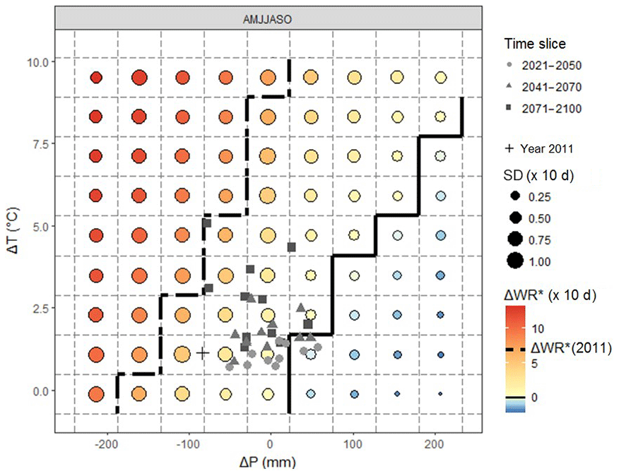
Figure 12Climate response surface of legally binding water-restriction-level anomalies ΔWR* for the Ouche river basin, including both exposure and performance characterizations.
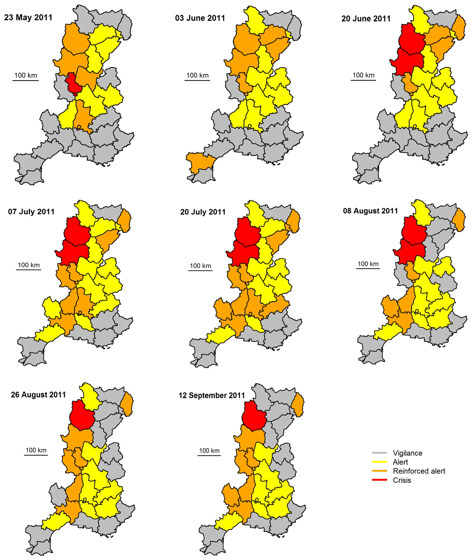
Figure 13Most severe water-restriction level adopted at the department-level scale for several dates between May and September 2011 (source: French Ministry of Ecology).
5.4 A regional perspective for prioritizing adaptation strategies
Following the methodology applied to the Ouche river basin, ΔWR* (2011) values were calculated for individual catchments and averaged to produce a value of Tc relevant for each class (Table 7). Class variation in ΔWR* (2011) is large, with Class 2 and 3 showing thresholds of at least seven 10 d periods, whilst they are close to zero for Class 1 and Class 4. The scatter in the ΔWR* (2011) values is certainly due to heterogeneity in crops, in irrigation systems, in climate conditions, etc., at the regional scale, leading to locally differentiated sensitivity to water restrictions as well as to biases in WR modelling. Since information on agricultural disaster notifications is only available for the year 2011, it is difficult to come to conclusions on the origins of the dispersion (natural or non-natural). However the distribution and absolute values of the critical thresholds reflect the spatial pattern of WR enforced from May to September 2011 well, with southern regions and the French Alps moderately affected by lack of rainfall in spring compared to the northern and western regions of the RM district (Fig. 13). Surprisingly negative values for ΔWR* (2011) are found for some catchments of Class 1 and 4, providing no evidence to support their agricultural disaster status that year. At the RM scale, average ΔWR* (2011) equals 38 d when considering all catchments and increases to 66 d when considering only catchments under agricultural disaster status. Simplified but realistic assumptions are imposed by the lack of detailed information; thus only one value was considered at the regional scale despite high dispersion in ΔWR* (2011) values (Table 7): the critical threshold Tc was set to the average of the ΔWR* (2011) values computed on all catchments in departments under agricultural disaster status in 2011 (6.6 10 d periods) and was used thereafter for all classes. Note that this value of Tc seems realistic: it represents a significant period with restrictions (66 d or 30 % of the time between 1 April and 31 October).
Table 7Summary statistics for the mean anomaly ΔWR* (2011) and for the measure of vulnerability (VI) estimated at the regional scale.
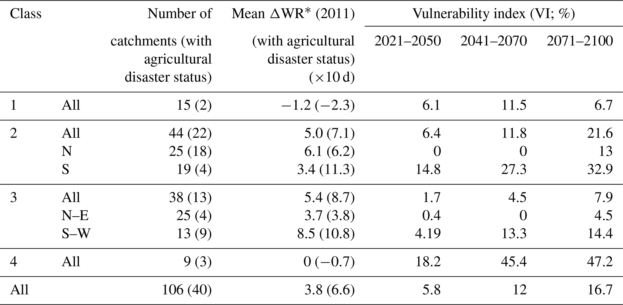
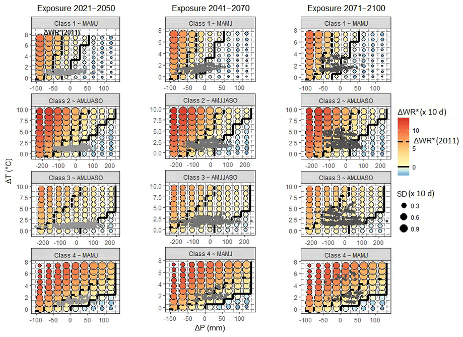
Figure 14Representative climate response surfaces for each class, including both exposure and performance characterizations.
Using the class WR response surface as a diagnostic tool, exposure information (grey symbols) and thresholds (ΔWR, solid; ΔWR* (2011), dashed black lines) were displayed (Fig. 14), and the VI was calculated (Table 7). The location of the two isopleths ΔWRWR* (2011) (black dotted line) and ΔWR (black straight line) in the WR response surface depends on the shape of the response surface and differs from one class to another. The portion of the WR response surface associated with ΔWR is gradually lower from Class 1 to Class 4, suggesting that catchments of Class 4 are more subject to an increase in water-restriction occurrence than catchments of the other classes. Class 1 and 4, the most extreme responses classes, contain fewer catchments, whilst Class 2 and 3, characterized by an intermediate response, have the most of the catchments. Because of the large geographical spread of catchments of Class 2 and 3, an expert-based division was done to distinguish catchments with continental (northern sectors, Class 2-N) and Mediterranean (southern sectors, Class 2-S) climate in terms of exposure. This is to better capture the predominantly north–south gradient in future projections of both temperature and rainfall, as they have a differing impact on the river flow regime (e.g. Boé et al., 2009; Chauveau et al., 2013; Dayon et al., 2018). For all classes, vulnerability increases with lead time, with Class 4 showing the largest vulnerability and Class 1 being the less vulnerable despite its location in the Mediterranean area. In Class 2 and 3, vulnerability increases from north to south in the RM district (VI = 13 % for Class 2-N compared to 32.9 % for Class 2-S at the end of the century). These contrasting results are mainly explained by the difference between exposure characterizations, since a common value of the threshold Tc was adopted.
5.5 Water-restriction policy implementation
In 2011, France adopted a general framework for action – the “French National Climate Change Impact Adaptation Plan” (“Plan National d'Adaptation au Changement Climatique – PNACC” in French) – with numerous recommendations related to research and observation. Five priorities of the first “PNACC” related to water resources have been highlighted. The “PNACC” was recently reviewed, and the “PNACC2” published in December 2018 confirms the place of DMPs as tools for monitoring water resources and water allocation and for driving greater public and stakeholder awareness (https://www.ecologique-solidaire.gouv.fr/adaptation-france-au-changement-climatique, last access: 1 August 2019).
However, until now, impacts of future climate change are not accounted for in DMPs. The development of DMPs has helped to ease past conflicts at the departmental scale. Water users are now facing more frequent water restrictions – more than half of France has departments experiencing WRL ≥ 1 between 2011 and 2018 (Fig. 15) – and the timing and the level of the restrictions vary from one year to another: the highest number of French departments with WRL ≥ 1 was observed in summer in both 2015 and 2017, while the year 2018 was characterized by late water restrictions (mostly in autumn). Stakeholders are now questioning the DMP implementation but only in the short term – the impact of climate change is not yet a topic. One of their main concerns is the heterogeneity in current restriction levels and timing from one department to another or from the upstream to the downstream part of the catchment. One of the options being considered to address this challenge in southeastern France is to harmonize the definition of the regulatory thresholds at the regional scale. Results obtained here show that the standardization will probably not fix the problem due to the balance between sociopolitical and hydrological factors in the final WR statement.
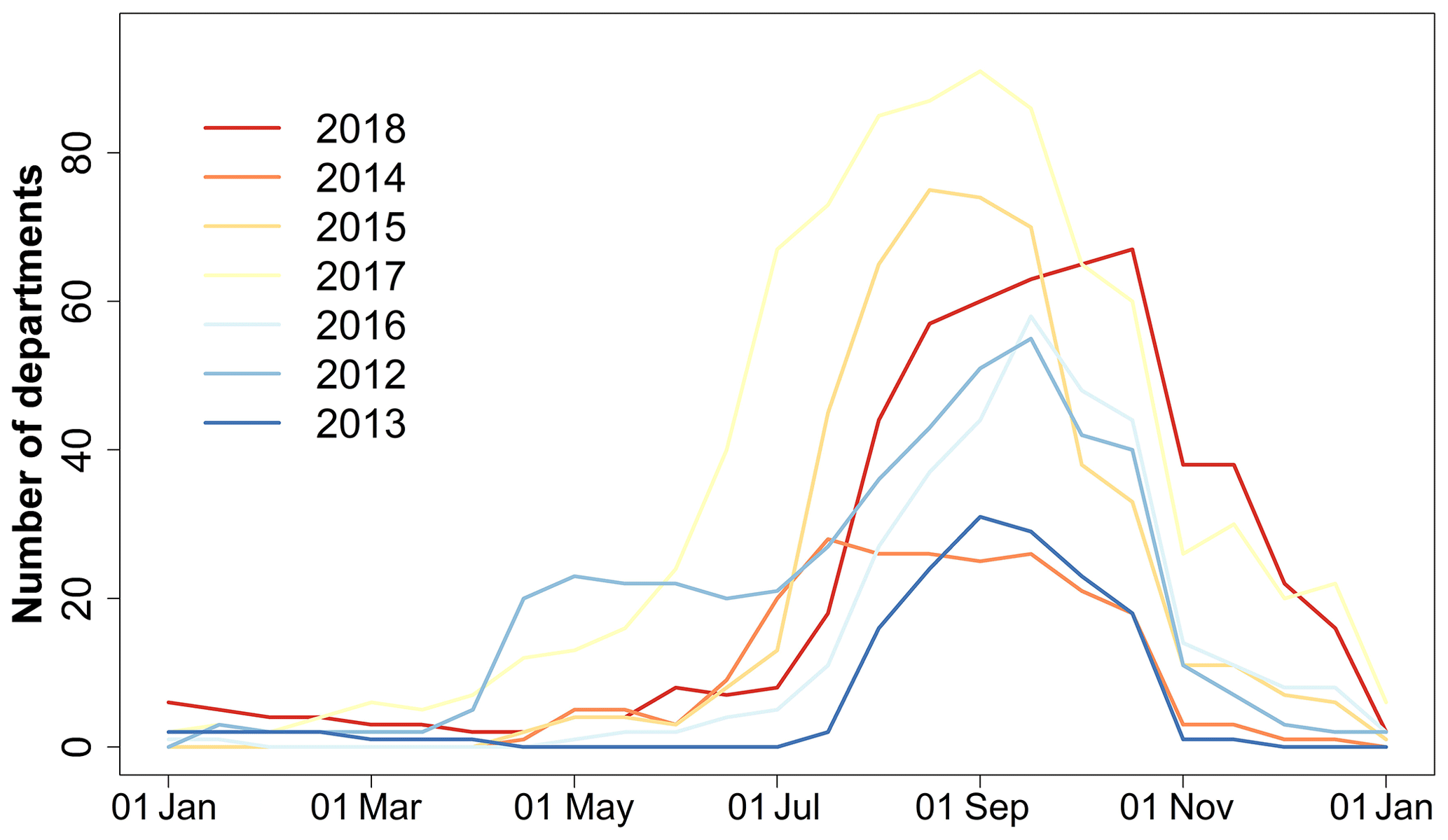
Figure 15Number of departments with at least one sub-catchment with WRL ≥ 1. The colour of the curves is associated to the annually averaged air temperature rank for France – from red to blue for the warmest (2018) to the coldest (2013) year – (sources: Météo-France and French ministry of Ecology).
The map displaying the class membership could be a convenient tool for local authorities to discuss the spatial heterogeneity in terms of impact to drought on water restrictions under both current and future climate conditions. Despite operating rules uniformly applied, there is high variability in catchment responses within the department (see the southernmost department in Fig. 10). Therefore, any investigation on DMPs at the department level disregarding this heterogeneity will be biased. The sensitivity analysis provides information for local authorities to better understand the differences in catchment responses to observed droughts in areas, which fall within their responsibility. For instance, water management in basins of Class 4 could be more problematic during a year with a severe heat wave, while it could be more problematic for a year with a pronounced precipitation deficit for catchments of Class 1. It is likely that the differences in the impact of droughts on WR will persist if stakeholders do not question the assumption of a uniform definition for the hydrological indicators within the department.
DMPs have been recognized in the “PNACC” as relevant water management tools, and our findings also have implications for adaptation strategies. We have shown that the climate change effects could be felt more acutely during the irrigation period by an increase in water restriction. Thus, relying on surface water to compensate deficits is highly hazardous. Options under consideration are saving water, enhancing water storage by building new small dams or securing water access by transferring water from the Rhône river (e.g. Ruf, 2012), which is considered to be an “overabundant” river within the RM district. Saving water is the solution favoured by the RM Water Agency. Creating new storages is increasingly considered to be a potential solution to secure water for agriculture, since they are not subject to water restrictions. Authorizing new water storages may also reduce the sense of unfairness among users in areas with no secured access. Most of the small reservoirs are filled by surface water in winter, release water later in summer for irrigation purposes and then limit the pressure on water resources during crises. However, there is actually a wide discussion about these hydraulic structures in France, since their cumulative impacts on the ecosystem and their efficiency are not well known (Habets et al., 2018). Building adaptation strategies for additional water storage may lead to maladaptation, since natural inflows will probably decrease and delay the mutation of agricultural practices and conservation measures. In addition, there is actually no guarantee that these reservoirs will be filled and that their storage capacity will be enough to cope with severe droughts.
The RM Water Agency has taken other the objectives of “PNACC” at the regional scale and has initiated an unprecedented major initiative that provides guidance for the “River Basin Management Plan” (2016–2021). The adaptation strategy partly relies on an analysis of the vulnerability in different water-related sectors (water resources, soil-moisture, biodiversity and water quality) within the RM district to climate change. The study complements this former analysis by focusing here on agricultural uses and meets the requirements for vulnerability assessment carried out by the RM Water Agency: it covers the same area, and the methodology is uniformly applied across the area of interest. It may help the RM Water Agency in identifying when and where actions and investments are the most needed to mitigate the effects of climate change (probably in catchments of Class 4 from the short perspective and later for the other areas).
This paper presents a first attempt to analyse and simulate water restrictions over a large area in France, applying an alternative approach to the classical top-down approach. The risk-based approach developed here relies on sensitivity-based analyses to a wide range of climate changes, making it scenario-neutral. However ex ante climate projections are introduced in the last stage of the framework to assess the likelihood of failure.
The analysis of the past and current DMPs in the RM district shows decision-making processes that are highly heterogeneous in terms of both the low-flow monitoring variable and regulatory thresholds. In reality, the WR statements follow a set of rules defined in the DMPs (which can be simulated and reproduced automatically) but also expert judgment or lobbying from key stakeholders – which are not accounted for in the WRL modelling framework put in place here. However, the post-processing of GR6J outputs allows for the detection of more than 68 % of severe alerts (more severe than level 1), making the developed framework a useful tool. Our study is a first step towards a comprehensive accounting of physical processes but does not capture socio-economic factors, also critically important, and reaches out with interdisciplinarity for completing the modelling framework designed here. The study at the regional scale illustrates an expected difficulty to simulate accurately a regulatory framework. Further improvement is not expected in enhancing hydrological models but in reproducing decision-making processes. The overall performance could be improved by scrutinizing the reports of the drought committees to better understand the weight of the stakeholders in the final statement.
The sensitivity analysis and the related response surfaces suggest that basins located in the southern Alps are the most responsive basins to climate change and that those experiencing a high ratio P / PET are found to be the less responsive. The classification method CART has been applied to 106 responses surfaces associated with 106 gauged basins and leads to four classes with different sensitivity. The key variables known at unmodelled but gauged catchments can be introduced in the decision tree to finally predict the assignment as a first guess to one of the four classes. Water managers are thus encouraged to monitor, with priority, more accurately temperature and/or precipitation when and where the sensitivity of their catchments is found the highest. This may mean efforts to reinforce field instrumentation within these key catchments.
Although incomplete, the proposed framework demonstrates, as expected (see Assessment Box SPM.2 in Table 1 in IPCC, 2014), a sensitivity of the DMPs to climate changes. The impact of climate change on the river flow is expected to be gradual, thus offering opportunities to update, to harmonize and to adapt DMPs to changes in climate conditions and water needs. As a consequence, the need for adaptation of existing drought action plans could differ greatly from one catchment to another and should take into account intrinsic sensitivity to climate change aside from top-down projections. Results also show the need to firstly adapt DMPs in temperature-sensitive catchments more subject to a significant increase in legally binding restrictions in the short term. In contrast, the capacity to anticipate changes in both the occurrence and severity of WR, and their consequences for water management, will be challenging in catchments where water restrictions are mainly driven by precipitation due to their high uncertainties in future regional climate projections.
The risk-based approach was applied to assess the vulnerability of irrigation due to regulatory instruments under modified climate. Evaluating the impact of climate change on irrigation was not the objective of the suggested framework; it was applied to estimate the likelihood of failure for irrigation at various lead times instead. Usually, a failure is when irrigation water needs are not fully satisfied. This case study suggests the use of a proxy obtained from a national system of compensation to define a critical threshold (maximum acceptable duration with water restriction). Analysis, however, was based on limited data (1 year), and a better failure assessment is required using other years (e.g. 2015 and 2017). The higher the probability, the more vulnerable the irrigation use within the department. Finally, socio-economic system stressors like agricultural practices, population growth, water demand, etc., should be considered to highlight combinations that would lead to unacceptable conditions and to assess the performance of various adaptation strategies under an extended set of future climate conditions (Poff et al., 2016).
Climate response surface appears to be a convenient tool for simulating and discussing future perspectives locally on the basin scale or more broadly on a given management territory. For example, they can support implement adaptive strategies (see – as an example – the robust decision-making framework suggested by Lempert and Groves, 2010): response surfaces can be drawn for different adaptation scenarios combined with periodic updates of DMPs, including rules for defining regulatory thresholds, monitoring variables evolving over time, etc.
Note that all results are based on a single hydrological model, but a multi-model approach could be applied, as the magnitude of the rainfall–runoff response was shown to vary with different hydrological models (e.g. Vidal et al., 2016; Kay et al., 2014). Finally, an extension of the area of interest to the whole of France may bring to light a more complete typology of response surfaces and a wider range of sensitivity.
Regional climate model (RCM) projections were obtained from the DRIAS portal (http://drias-climat.fr/, last access: November 2016) and consulted on November 2016. Analyses were performed in R (R Core Team, 2016), with packages airGR (Coron et al., 2017), chron (James and Hornik, 2017), circular (Lund et al., 2017), doParallel (Calaway et al., 2017), dplyr (Wickham and François, 2015), ggplot2 (Wickham, 2009), hydroTSM (Zambrano-Bigiarini, 2014), RColorBrewer (Neuwirth, 2014), reshape2 (Wickham, 2017), rpart (Therneau et al., 2018), scales (Wickham, 2016), stringr (Wickham, 2017) and zoo (Zeileis and Grothendieck, 2005).
Sauquet et al. (2008) have defined a classification based on the mean monthly runoff pattern (Fig. A1), and a map was published showing the assignment to one class along the main river network.
Group 1 to 6 are pluvial river flow regimes. The six groups mainly differ by the contrast between the maximum and the minimum of the monthly discharges. Nearly uniform flows through most of the year (Group 1) are found where large aquifers moderate flows, whereas Group 6 is characterized by very low flow in summer, reflecting the lack of deep groundwater storages in the catchment. Group 7 is representative of Mediterranean river flow regimes, where small rivers basins experience hot and dry summers and intense rainy events in autumn. Their runoff pattern therefore exhibits a severe low flow in summer and high flow in November. In mountainous areas, the uppermost basins display snowmelt-fed regimes (Group 10–12). The lower the outlet, the lower the contributions of snowmelt to runoff. Group 8 to 9 are in the transition regime. The seasonal variation in streamflow is affected as much by precipitation timing as by air temperature and topographic influences (on snowpack formation and snowmelt timing). Typically, high flows are observed in spring.
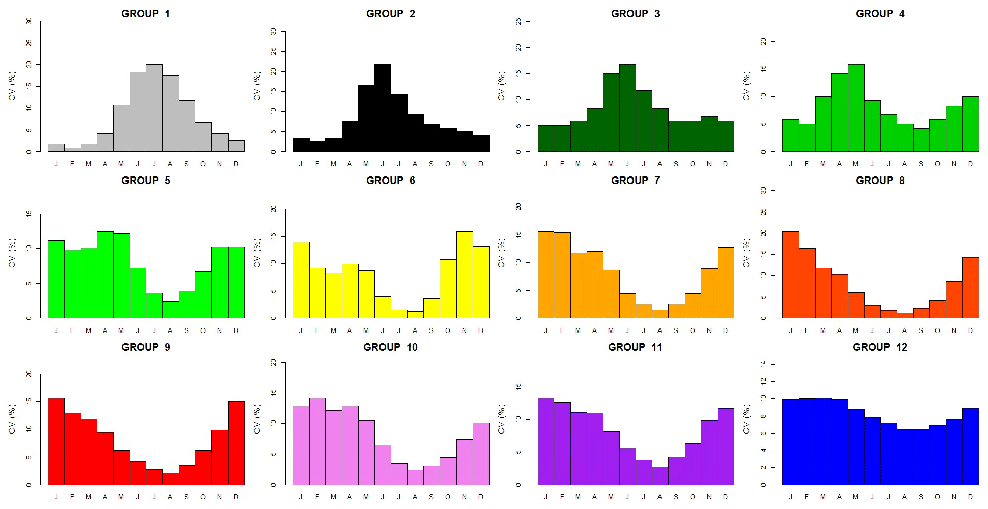
Figure A1Reference dimensionless hydrographs representative of the classification of river flow regime for France (after Sauquet et al., 2008).The 12 dimensionless coefficients CM are the 12 values of mean monthly runoff (mm) divided by the mean annual runoff.
ES and CP jointly developed the general framework. BR and AD carried out most of the simulations. BR and ES prepared the graphs and the tables. All authors contributed to the analysis and the discussion.
The authors declare that they have no conflict of interest.
The authors thank Météo-France for providing access to the Safran database. We thank Jan Seibert as well as the anonymous reviewers for their critical but very constructive comments.
This research was partly funded by the Rhône-Méditerranée-Corse Water Agency.
This paper was edited by Roberto Greco and reviewed by Brunella Bonaccorso and two anonymous referees.
Andrew, J. T. and Sauquet, E.: Climate Change Impacts and Water Management Adaptation in Two Mediterranean-Climate Watersheds: Learning from the Durance and Sacramento Rivers, Water, 9, 126, https://doi.org/10.3390/w9020126, 2017.
Arnell, N. W.: Relative effects of multi-decadal climatic variability and changes in the mean and variability of climate due to global warming: future streamflow in Britain, J. Hydrol., 270, 19–213, 2003.
Barbier, R., Barreteau, O., and Breton, C.: Management of water scarcity: between negotiated implementation of the “décret sécheresse” and emergence of local agreements, Ingénieries – EAT IRSTEA édition 2007, 3–19, 2007.
Beaufort, A., Lamouroux, N., Pella, H., Datry, T., and Sauquet, E.: Extrapolating regional probability of drying of headwater streams using discrete observations and gauging networks, Hydrol. Earth Syst. Sci., 22, 3033–3051, https://doi.org/10.5194/hess-22-3033-2018, 2018.
Bisselink, B., Bernhard, J., Gelati, E., Adamovic, M., Guenther, S., Mentaschi, L. and De Roo, A.: Impact of a changing climate, land use, and water usage on Europe's water resources, EUR 29130 EN, Publications Office of the European Union, Luxembourg, JRC110927, ISBN 978-92-79-80287-4, https://doi.org/10.2760/847068, 2018.
Boé, J., Terray, L., Martin, E., and Habets, F.: Projected changes in components of the hydrological cycle in French river basins during the 21st century, Water Resour. Res., 45, W08426, https://doi.org/10.1029/2008WR007437, 2009.
Breiman, L., Friedman, J. H., Olshen, R., and Stone, C. J.: Classification and Regression Trees, Wadsworth, Belmont, California, 1984.
Brekke, L. D., Maurer, E. P., Anderson, J. D., Dettinger, M. D., Townsley, E. S., Harrison, A., and Pruitt, T.: Assessing reservoir operations risk under climate change, Water Resour. Res., 45, W04411, https://doi.org/10.1029/2008WR006941, 2009.
Broderick, C., Murphy, C., Wilby, R. L., Matthews, T., Prudhomme, C., and Adamson, M.: Using a Scenario – neutral framework to avoid potential maladaptation to future flood risk, Water Resour. Res., 55, 1079–1104, https://doi.org/10.1029/2018WR023623, 2019.
Brown, C. and Wilby, R. L.: An alternate approach to assessing climate risks, Trans. Am. Geophys. Un., 93, 401–402, 2012.
Brown, C., Werick, W., Leger, W., and Fay, D.: A decision-analytic approach to managing climate risks: Application to the upper great lakes, J. Am. Water Resour. Assoc., 47, 524–534, 2011.
Brown, C., Ghile, Y., Laverty, M., and Li, K.: Decision scaling: Linking bottom-up vulnerability analysis with climate projections in the water sector, Water Resour. Res., 48, W09537, https://doi.org/10.1029/2011WR011212, 2012.
Bubnová, R., Hello, G., Bénard, P., and and Geleyn, J. F.: Integration of the Fully Elastic Equations Cast in the Hydrostatic Pressure Terrain-Following Coordinate in the Framework of the ARPEGE/Aladin NWP System, Mon. Weather Rev., 123, 515–535, 1995.
Caillouet, L., Vidal, J.-P., Sauquet, E., Devers, A., and Graff, B.: Ensemble reconstruction of spatio-temporal extreme low-flow events in France since 1871, Hydrol. Earth Syst. Sci., 21, 2923–2951, https://doi.org/10.5194/hess-21-2923-2017, 2017.
Calaway, R., Microsoft Corporation, Weston, S., and Tenenbaum, D.: doParallel: Foreach Parallel Adaptor for the `parallel' Package, R package version 1.0.11, available at: https://CRAN.R-project.org/package=doParallel, last access: 1 October 2017.
Chauveau, M., Chazot, S., Perrin, C., Bourgin, P.-Y., Sauquet, E., Vidal, J.-P., Rouchy, N., Martin, E., David, J., Norotte, T., Maugis, P., and de Lacaze, X.: What will be the impacts of climate change on surface hydrology in France by 2070?, La Houille Blanche, 4, 5–15, 2013.
Cipriani, T., Tilmant, F., Branger, F., Sauquet, E., and Datry, T.: Impact of climate change on aquatic ecosystems along the Asse river network, in: Hydrology in a Changing World: Environmental and Human Dimensions, edited by: Daniell, T., AIHS Publ., 363, 463–468, 2014.
Collet, L., Harrigan, S., Prudhomme, C., Formetta, G., and Beevers, L.: Future hot-spots for hydro-hazards in Great Britain: a probabilistic assessment, Hydrol. Earth Syst. Sci., 22, 5387–5401, https://doi.org/10.5194/hess-22-5387-2018, 2018.
Coron, L., Thirel, G., Delaigue, O., Perrin, C., and Andréassian, V.: airGR: A Suite of Lumped Hydrological Models in an R-Package, Environ. Model. Softw., 94, 166–171, https://doi.org/10.1016/j.envsoft.2017.05.002, 2017.
Culley, S., Noble, S., Yates, A., Timbs, M., Westra, S., Maier, H. R., Giuliani, M., and Castelletti A.: A bottom-up approach to identifying the maximum operational adaptive capacity of water resource systems to a changing climate, Water Resour. Res., 52, 6751–6768, 2016.
Danner, A., Mohammad Safeeq, G., Grant, G. E., Wickham, C., Tullos, D., and Santelmann, M. V.: Scenario-Based and Scenario-Neutral Assessment of Climate Change Impacts on Operational Performance of a Multipurpose Reservoir, J. Am. Water Resour. Assoc., 53, 1467–1482, 2017.
Dayon, G., Boé, J., Martin, E., and Gailhard, J.: Impacts of climate change on the hydrological cycle over France and associated uncertainties, Comptes Rendus Geoscience, 350, 141–153, 2018.
Fronzek, S., Carter, T. R., and Räisänen, J.: Applying probabilistic projections of climate change with impact models: a case study for sub-arctic palsa mires in Fennoscandia, Climatic Change, 99, 515–534, 2010.
Ghile Y. B., Taner, M. Ü., Brown, C., and Talbi, A.: Bottom-up climate risk assessment of infrastructure investment in the Niger River Basin, Climatic Change, 122, 97–110, 2014.
Giorgi, F.: Climate change hot-spots, Geophys. Res. Lett., 33, L08707, https://doi.org/10.1029/2006GL025734, 2006.
Grouillet, B., Fabre, J., Ruelland, D., and Dezetter, A.: Historical reconstruction and 2050 projections of water demand under anthropogenic and climate changes in two contrasted Mediterranean catchments, J. Hydrol., 522, 684–696, 2015.
Guo, D., Westra, S., and Maier, H. R.: An inverse approach to perturb historical rainfall data for scenario-neutral climate impact studies, J. Hydrol., 556, 877–890, 2016.
Guo, D., Westra ,S., and Maier, H. R.: Use of a scenario-neutral approach to identify the key hydrometeorological attributes that impact runoff from a natural catchment, J. Hydrol., 554, 317–330, https://doi.org/10.1016/j.jhydrol.2017.09.021, 2017.
Gupta, H. V., Kling, H., Yilmaz, K., and Martinez, G. F.: Decomposition of the mean squared error and NSE performance criteria: Implications for improving hydrological modelling, J. Hydrol., 377, 80–91, https://doi.org/10.1016/j.jhydrol.2009.08.003, 2009.
Habets, F., Molénat, J., Carluer, N., Douez, O., and Leenhardt, D.: The cumulative impacts of small reservoirs on hydrology: A review, Sci. Total Environ., 643, 850–867, https://doi.org/10.1016/j.scitotenv.2018.06.188, 2018.
Hellwig, J. and Stahl, K.: An assessment of trends and potential future changes in groundwater-baseflow drought based on catchment response times, Hydrol. Earth Syst. Sci., 22, 6209–6224, https://doi.org/10.5194/hess-22-6209-2018, 2018.
Hublart, P., Ruelland, D., García de Cortázar-Atauri, I., Gascoin, S., Lhermitte, S., and Ibacache, A.: Reliability of lumped hydrological modeling in a semi-arid mountainous catchment facing water-use changes, Hydrol. Earth Syst. Sci. 20, 3691–3717, https://doi.org/10.5194/hess-20-3691-2016, 2016.
IPCC: Summary for policymakers, in: Climate Change 2014: Impacts, Adaptation, and Vulnerability. Part A: Global and Sectoral Aspects, Contribution of Working Group II to the Fifth Assessment Report of the Intergovernmental Panel on Climate Change, edited by: Field, C. B., Barros, V. R., Dokken, D. J., Mach, K. J., Mastrandrea, M. D., Bilir, T. E., Chatterjee, M., Ebi, K. L., Estrada, Y. O., Genova, R. C., Girma, B., Kissel, E. S., Levy, A. N., MacCracken, S., Mastrandrea, P. R., and White, L. L., Cambridge University Press, Cambridge, UK and New York, NY, USA, 1–32, 2014.
Jacob, D., Petersen, J., Eggert, B., Alias, A., Christensen, O. B., Bouwer, L. M., and Braun, A.: EURO-CORDEX: New high-resolution climate change projections for European impact research, Reg. Environ. Change, 14, 563–578 https://doi.org/10.1007/s10113-013-0499-2, 2014.
Jakeman, A. J., Littlewood, I. G., and Whitehead, P. G.: Computation of the instantaneous unit hydrograph and identifiable component flows with application to two small upland catchments, J. Hydrol., 117, 275–300, 1990.
James, D. and Hornik, K.: chron: Chronological Objects which Can Handle Dates and Times, R package version 2.3-50, available at: https://CRAN.R-project.org/package=chron, last access: 1 October 2017.
Jiménez Cisneros, B. E., Oki, T., Arnell, N. W., Benito, G., Cogley, J. G., Döll, P., Jiang, T., and Mwakalila, S. S.: Freshwater resources, in: Climate Change 2014: Impacts, Adaptation, and Vulnerability. Part A: Global and Sectoral Aspects, Contribution of Working Group II to the Fifth Assessment Report of the Intergovernmental Panel on Climate Change, edited by: Field, C. B., Barros, V. R., Dokken, D. J., Mach, K. J., Mastrandrea, M. D., Bilir, T. E., Chatterjee, M., Ebi, K. L., Estrada, Y. O., Genova, R. C., Girma, B., Kissel, E. S., Levy, A. N., MacCracken, S., Mastrandrea, P. R., and White, L. L., Cambridge University Press, Cambridge, UK and New York, NY, USA, 229–269, 2014.
Jolliffe, I. T. and Stephenson, D. B.: Forecast verification. A practitioner's Guide in Atmospheric Science, John Wiley & Sons Ltd, Chichester, 2003.
Kay, A. L., Crooks, S. M., and Reynard, N. S.: Using response surfaces to estimate impacts of climate change on flood peaks: assessment of uncertainty, Hydrol. Process., 28, 5273–5287, https://doi.org/10.1002/hyp.10000, 2014.
Kondolf, G. M., Podolak, K., and Grantham, T. E.: Restoring mediterranean-climate rivers, Hydrobiologia, 719, 527–545, https://doi.org/10.1007/s10750-012-1363-y, 2013.
Köplin, N., Schädler, B., Viviroli, D., and Weingartner, R.: Relating climate change signals and physiographic catchment properties to clustered hydrological response types, Hydrol. Earth Syst. Sci., 16, 2267–2283, https://doi.org/10.5194/hess-16-2267-2012, 2012.
Le Moine, N.: Le bassin versant de surface vu par le souterrain: une voie d'amélioration des performances et du réalisme des modéles pluie-débit?, PhD thesis, Université Pierre et Marie Curie, Paris, Cemagref, Antony, 324 pp., 2008.
Lémond, J., Dandin, P., Planton, S., Vautard, R., Pagé, C., Déqué, M., Franchistéguy, L., Geindre, S., Kerdoncuff, M., Li, L., Moisselin, J. M., Noël, T., and Tourre, Y. M.: DRIAS: a step toward Climate Services in France, Adv. Sci. Res., 6, 179–186, https://doi.org/10.5194/asr-6-179-2011, 2011.
Lempert, R. J. and Groves, D. G.: Identifying and evaluating robust adaptive policy responses to climate change for water management agencies in the American west, Technol. Forecast. Social Change, 77, 960–974, https://doi.org/10.1016/j.techfore.2010.04.007, 2010.
Lund, U., Agostinelli, C., Arai, H., Gagliardi, A., Garcia Portugues, E., Giunchi, D., Irisson, J. O., Pocernich, M., and Rotolo, F.: circular: Circular Statistics, R package version 0.4-93, available at: https://CRAN.R-project.org/package=circular (last access: 1 August 2019), 2017.
Lyne, V. and Hollick, M.: Stochastic time variable rainfall runoff modeling, in: Proceedings of the Hydrology and Water Resources Symposium Berth, 1979, National Committee on Hydrology and Water Resources of the Institution of Engineers, Australia, 89–92, 1979.
Mastrandrea, M. D., Heller, N. E., Root, T. L., and Schneider, S. H.: Bridging the gap: linking climate-impacts research with adaptation planning and management, Climatic Change, 100, 87–101, 2010.
MEDDE – Ministère de l'Ecologie et du Développement Durable, Plan d'Action Sécheresse, available at: http://www.rhone-mediterranee.eaufrance.fr/docs/infos-secheresse/gestion-secheresse/2004/PAS_2004.pdf (last access: 1 August 2019), 2004.
Nash, J. E. and Sutcliffe, J. V.: River flow forecasting through conceptual models Part I – A discussion of principles, J. Hydrol., 10, 282–290, 1970.
Neuwirth, E.: RColorBrewer: ColorBrewer Palettes, R package version 1.1-2, available at: https://CRAN.R-project.org/package=RColorBrewer (last access: 1 August 2019), 2014.
Oudin, L., Hervieu, F., Michel, C., Perrin, C., Andréassian, V., Anctil, F., and Loumagne, C.: Which potential evapotranspiration input for a lumped rainfall–runoff model?: Part 2 – towards a simple and efficient potential evapotranspiration model for rainfall–runoff modelling, J. Hydrol., 303, 290–306, 2005.
Paeth, H., Vogt, G., Paxian, A., Hertig, E., Seubert, S., and Jacobeit, J.: Quantifying the evidence of climate change in the light of uncertainty exemplified by the Mediterranean hot spot region, Global Planet. Change, 151, 144–151, 2017.
Paton, F., Maier, H., and Dandy, G.: Relative magnitudes of sources of uncertainty in assessing climate change impacts on water supply security for the southern Adelaide water supply system, Water Resour. Res., 49, 1643–1667, 2013.
Perrin, C., Michel, C., and Andréassian, V.: Improvement of a parsimonious model for streamflow simulation, J. Hydrol., 279, 275–289, 2003.
Poff, N. L., Brown, C. M., Grantham, T. E., Matthews, J. H., Palmer, M. A., Spence, C. M., Wilby, R. L., Haasnoot, M., Mendoza, G. F., Dominique, K. C., and Baeza, A.: Sustainable water management under future uncertainty with eco-engineering decision scaling, Nat. Clim. Change, 6, 25–34, 2016.
Poncelet, C., Merz, R., Merz, B., Parajka, J., Oudin, L., Andréassian, V., and Perrin, C.: Process-based interpretation of conceptual hydrological model performance using a multinational catchment set, Water Resour. Res., 53, 7247–7268, 2017.
Prudhomme, C., Wilby, R. L, Crooks, S., Kay, A. L., and Reynard, N. S.: Scenario-neutral approach to climate change impact studies: Application to flood risk, J. Hydrol., 390, 198–209, 2010.
Prudhomme, C., Kay, A., Crooks, S., and Reynard, N.: Climate change and river flooding: Climate change and river flooding: Part 1 classifying the sensitivity of British catchments, Climatic Change, 119, 933–948, 2013a.
Prudhomme, C., Kay, A., Crooks, S., and Reynard, N.: Climate change and river flooding: Part 2 sensitivity characterization for British catchments and example vulnerability assessments, Climatic Change, 119, 949–964, 2013b.
Prudhomme, C., Sauquet, E., and Watts, G.: Low flow response surfaces for drought decision support: A case study from the UK, J. Extr. Events, 2, 1550005, https://doi.org/10.1142/S2345737615500050, 2015.
Pushpalatha, R., Perrin, C., Le Moine, N., Mathevet, T., and Andréassian, V. A downward structural sensitivity analysis of hydrological models to improve low-flow simulation, J. Hydrol., 411, 66–76, 2011.
Quintana-Seguí, P., Le Moigne, P., Durand, Y., Martin, E., Habets, F., Baillon, M., Canellas, C., Franchistéguy, L., and Morel, S.: Analysis of near-surface atmospheric variables: validation of the safran analysis over France, J. Appl. Meteorol. Clim., 47, 92–107, 2008.
Radnoti, G.: Comments on A Spectral Limited-Area Formulation with Time-Dependent Boundary Conditions Applied to the Shallow-Water Equations, Mon. Weather Rev., 123, 3122–3123, 1995.
Ray, P. A. and Brown, C. M. Confronting Climate Uncertainty in Water Resources Planning and Project Design: The Decision Tree Framework, World Bank, Washington, D.C., 2015.
R Core Team: R: A Language and Environment for Statistical Computing, R Foundation for Statistical Computing, Vienna, Austria, available at: https://www.R-project.org/ (last access: 1 August 2019), 2016.
Rousseeuw, P. J.: Silhouettes: A graphical aid to the interpretation and validation of cluster analysis, J. Comput. Appl. Math., 20, 53–65, 1987.
Ruf, T.: Le projet Aqua Domitia: intérêt et limites, Pour, 2012/1, 65–74, https://doi.org/10.3917/pour.213.0065, 2012.
Samaniego, L., Thober, S., Kumar, R., Wanders, N., Rakovec, O., Pan, M., Zink, M., Sheffield, J., Wood, E. F., and Marx, A.: Anthropogenic warming exacerbates European soil moisture droughts, Nat. Clim. Change, 8, 421–426, https://doi.org/10.1038/s41558-018-0138-5, 2018.
Sauquet, E.: Mapping mean annual river discharges: geostatistical developments for incorporating river network dependencies, J. Hydrol., 331, 300–314, 2006.
Sauquet, E. and Catalogne, C.: Comparison of catchment grouping methods for flow duration curve estimation at ungauged sites in France, Hydrol. Earth Syst. Sci., 15, 2421–2435, https://doi.org/10.5194/hess-15-2421-2011, 2011.
Sauquet, E., Gottschalk, L., and Krasovskaia, I.: Estimating mean monthly runoff at ungauged locations: an application to France, Hydrol. Res., 39, 403–423, 2008.
Sauquet, E., Arama, Y., BlancCoutagne, E., Bouscasse, H., Branger, F., Braud, I., Brun, J.-F., Cherel, J., Cipriani, T., Datry, T., Ducharne, A., Hendrickx, F., Hingray, B., Krowicki, F., Le Goff, I., Le Lay, M., Magand, C., Malerbe, F., Mathevet, T., Mezghani, A., Monteil, C., Perrin, C., Poulhe, P., Rossi, A., Samie, R., Strosser, P., Thirel, G., Tilmant, F., and Vidal, J.-P.: Water allocation and uses in the Durance River basin in the 2050s: Towards new management rules for the main reservoirs?, La Houille Blanche, 5, 25–31, 2016.
Schlef, K. E., Steinschneider, S., and Brown, C. M.: Spatiotemporal Impacts of Climate and Demand on Water Supply in the Apalachicola-Chattahoochee-Flint Basin, J. Water Resour. Plan. Manage., 144, 05017020, https://doi.org/10.1061/(ASCE)WR.1943-5452.0000865, 2018.
Simonovic, S. P.: A new methodology for the assessment of climate change impacts on a watershed scale, Current Science, 98, 1047–1055, 2010.
Singh, R., Wagener, T., Crane, R., Mann, M. E., and Ning, L.: A vulnerability driven approach to identify adverse climate and land use change combinations for critical hydrologic indicator thresholds: application to a watershed in Pennsylvania, USA, Water Resour. Res., 50, 3409–3427, 2014.
Skamarock, W., Klemp, J., Dudhia, J., Gill, D., Barker, D., Wang, W., Huang, X.-Y., and Duda, M.: A description of the advanced research WRF version 3, NCAR Technical Note NCAR/TN-475+STR, NCAR, Boulder, Colorado, USA, https://doi.org/10.5065/D68S4MVH, 2008.
Steinschneider, S. and Brown, C. M.: A semiparametric multivariate, multisite weather generator with low-frequency variability for use in climate risk assessments, Water Resour. Res., 49, 7205–7220, https://doi.org/10.1002/wrcr.20528, 2013.
Taylor, K. E., Stouffer, R. J., and Meehl, G. A.: An overview of CMIP5 and the experiment design, B. Am. Meteorol. Soc., 93, 485–498, 2012.
Terray, L. and Boé, J.: Quantifying 21st-century France climate change and related uncertainties, Comptes Rendus Geoscience, 345, 136–149, 2013.
Therneau, T., Atkinson, B., and Ripley, B.: rpart: Recursive Partitioning and Regression Trees, R package version 4.1-13, available at: https://CRAN.R-project.org/package=rpart (last access: 1 January 2019), 2018.
Touma, D., Ashfaq, M., Nayak, M. A., Kao, S.-C., and Diffenbaugh, N. S.: A multi-model and multi-index evaluation of drought characteristics in the 21st century, J. Hydrol., 526, 196–207, 2015.
UNEP: World Atlas of Desertification, The United Nations Environment Programme – UNEP, London, 1993.
Valéry, A., Andréassian, V., and Perrin, C.: `As simple as possible but not simple': What is useful in a temperature-based snow-accounting routine? Part 2 – Sensitivity analysis of the Cemaneige snow accounting routine on 380 catchments, J. Hydrol., 517, 1176–1187, 2014.
Van Loon, A. F., Gleeson, T., Clark, J., Van Dijk, A. I. J. M., Stahl, K., Hannaford, J., Di Baldassarre, G., Teuling, A. J., Tallaksen, L. M., Uijlenhoet, R., Hannah, D. M., Sheffield, J., Svoboda, M., Verbeiren, B., Wagener, T., Rangecroft, S., Wanders, N., and Van Lanen, H. A. J.: Drought in the Anthropocene, Nat. Geosci., 9, 89–91, 2016.
Vidal, J.-P., Martin, E., Franchistéguy, L., Baillon, M., and Soubeyroux, J.-M.: A 50-year high-resolution atmospheric reanalysis over France with the Safran system, Int. J. Climatol., 30, 1627–1644, 2010.
Vidal, J.-P., Hingray, B., Magand, C., Sauquet, E., and Ducharne, A.: Hierarchy of climate and hydrological uncertainties in transient low-flow projections, Hydrol. Earth Syst. Sci., 20, 3651–3672, https://doi.org/10.5194/hess-20-3651-2016, 2016.
Ward Jr., J.: Hierarchical grouping to optimize an objective function, J. Am. Stat. Assoc., 58, 236–244, 1963.
Weiß, M.: Future water availability in selected European catchments: a probabilistic assessment of seasonal flows under the IPCC A1B emission scenario using response surfaces, Nat. Hazards Earth Syst. Sci., 11, 2163–2171, https://doi.org/10.5194/nhess-11-2163-2011, 2011.
Wetterhall, F., Graham, L. P., Andréasson, J., Rosberg, J., and Yang, W.: Using ensemble climate projections to assess probabilistic hydrological change in the Nordic region, Nat. Hazards Earth Syst. Sci., 11, 2295–2306, https://doi.org/10.5194/nhess-11-2295-2011, 2011.
Whateley, S., Steinschneider, S., and Brown, C. M.: A climate change range-based method for estimating robustness for water resources supply, Water Resour. Res., 50, 8944–8961, 2014.
Wickham, H.: ggplot2: Elegant Graphics for Data Analysis, Hadley Wickham, Springer-Verlag, New York, 2009.
Wickham, H.: scales: Scale Functions for Visualization, R package version 0.4.0, available at: https://CRAN.R-project.org/package=scales (last access: 1 September 2019), 2016.
Wickham, H.: stringr: Simple, Consistent Wrappers for Common String Operations, R package version 1.2.0, available at: https://CRAN.R-project.org/package=stringr (last access: 1 March 2019), 2017.
Wickham, H. and Francois, R.: dplyr: A Grammar of Data Manipulation, R package version 0.4.3, available at: https://CRAN.R-project.org/package=dplyr (last access: 1 June 2019), 2015.
Zambrano-Bigiarini, M.: hydroTSM: Time series management, analysis and interpolation for hydrological modelling, R package version 0.4-2-1, available at: https://CRAN.R-project.org/package=hydroTSM (last access: 1 June 2019), 2014.
Zeileis, A. and Grothendieck, G.: zoo: S3 Infrastructure for Regular and Irregular Time Series. J. Stat. Softw., 14, 1–27, https://doi.org/10.18637/jss.v014.i06, 2005.
- Abstract
- Introduction
- Study area and materials
- Operating drought management plans in the Rhône–Mediterranean district
- Risk-based framework and the related tools
- Drought management plans under climate change and their impact on irrigation use
- Conclusions
- Data availability
- Appendix A: Classification of river flow regime for France
- Author contributions
- Competing interests
- Acknowledgements
- Financial support
- Review statement
- References