Quantifying thermal refugia connectivity by combining temperature modeling, distributed temperature sensing, and thermal infrared imaging

Watershed-scale stream temperature models are often one-dimensional because they require fewer data and are more computationally efficient than two- or three-dimensional models. However, one-dimensional models assume completely mixed reaches and ignore small-scale spatial temperature variability, which may create temperature barriers or refugia for cold-water aquatic species. Fine spatial- and temporal-resolution stream temperature monitoring provides information to identify river features with increased thermal variability. We used distributed temperature sensing (DTS) to observe small-scale stream temperature variability, measured as a temperature range through space and time, within two 400 m reaches in summer 2015 in Nevada's East Walker and main stem Walker rivers. Thermal infrared (TIR) aerial imagery collected in summer 2012 quantified the spatial temperature variability throughout the Walker Basin. We coupled both types of high-resolution measured data with simulated stream temperatures to corroborate model results and estimate the spatial distribution of thermal refugia for Lahontan cutthroat trout and other cold-water species. Temperature model estimates were within the DTS-measured temperature ranges 21 % and 70 % of the time for the East Walker River and main stem Walker River, respectively, and within TIR-measured temperatures 17 %, 5 %, and 5 % of the time for the East Walker, West Walker, and main stem Walker rivers, respectively. DTS, TIR, and modeled stream temperatures in the main stem Walker River nearly always exceeded the 21 ^∘C optimal temperature threshold for adult trout, usually exceeded the 24 ^∘C stress threshold, and could exceed the 28 ^∘C lethal threshold for Lahontan cutthroat trout. Measured stream temperature ranges bracketed ambient river temperatures by −10.1 to +2.3 ^∘C in agricultural return flows, −1.2 to +4 ^∘C at diversions, −5.1 to +2 ^∘C in beaver dams, and −4.2 to 0 ^∘C at seeps. To better understand the role of these river features on thermal refugia during warm time periods, the respective temperature ranges were added to simulated stream temperatures at each of the identified river features. Based on this analysis, the average distance between thermal refugia in this system was 2.8 km. While simulated stream temperatures are often too warm to support Lahontan cutthroat trout and other cold-water species, thermal refugia may exist to improve habitat connectivity and facilitate trout movement between spawning and summer habitats. Overall, high-resolution DTS and TIR measurements quantify temperature ranges of refugia and augment process-based modeling.

1 Introduction

Trout and salmon avoid heat stress by sheltering in thermal refugia, or pockets of cooler water, when stream temperatures are near upper thermal tolerances (Dunham et al., 2003; Sutton et al., 2007). Where stream temperatures are warming or where cold-water fish species are near the margins of their ranges, measuring stream temperatures at small temporal and spatial scales is important to quantify thermal refugia and stream temperature heterogeneity (Vatland et al., 2015). One-dimensional stream temperature models estimate longitudinal stream temperature changes at the watershed scale but are poor predictors of thermal micro-habitats. On the other hand, high-resolution temperature monitoring provides micro-habitat information but is typically conducted over small spatial extents and thus difficult to extrapolate to the watershed scale for management and restoration decisions.

Stream temperature models are useful for river management because they help decision-makers understand stream temperature dynamics and the potential impacts of restoration and management. Many one-dimensional temperature models exist and have been applied to understand the temperature effects of dams, reservoir re-operation, climate change, and restoration in systems all over the world (e.g., Bond et al., 2015; Elmore et al., 2016; Pelletier et al., 2006). Stream temperature models used in management are often one-dimensional because they are less data intensive and more computationally efficient than two- or three-dimensional models that account for temperature variability over channel width and depth. However, one-dimensional watershed-scale models do not identify river features like cold-water pools, lateral variability, or groundwater seeps that are smaller than the model spatial resolution (Null et al., 2017).

Distributed temperature sensing (DTS) and thermal infrared (TIR) imaging are sometimes used in conjunction with stream temperature models. DTS provides near-continuous temperature measurements in both time and space (Selker et al., 2006; Suárez et al., 2011). Raman spectra DTS is capable of measuring temperatures every meter along fiber-optic cables with an accuracy of at least ±0.1 ^∘C, and cables vary between approximately 1 and 10 km (Tyler et al., 2009). DTS has determined zones of groundwater influence (Hare et al., 2015; Selker et al., 2006; Suárez et al., 2011) and hyporheic exchange (Briggs et al., 2012). DTS data were used to calibrate and validate a 1.3 km physically based, one-dimensional stream temperature model of the Boiron de Morges River in southwest Switzerland (Roth et al., 2010) and a 580 m river reach in Luxembourg's Maisbich River (Westhoff et al., 2007). TIR imagery capture spatially continuous stream surface temperatures and have successfully identified spatial heterogeneity (Bingham et al., 2012; Fullerton et al., 2018) and located groundwater and tributary inputs (Dugdale et al., 2013; Loheide and Gorelick, 2006; Mundy et al., 2017). However, TIR data are for a single time unless acquired on multiple occasions (Dugdale, 2016; Torgersen et al., 2001). TIR data have been used in conjunction with stationary temperature loggers to calibrate reach- and basin-scale models (Bingham et al., 2012; Cardenas et al., 2014; Carrivick et al., 2012; Deitchman and Loheide, 2012). For example, TIR data were combined with instream temperature loggers to calibrate an 86 km QUAL2Kw water quality model in the Wenatchee River in Washington (Cristea and Burges, 2009) and a 100 km statistical model in the Big Hole River, MT, USA (Vatland et al., 2015). In the latter study, Vatland et al. (2015) concluded that point monitoring sites underestimate the temporal and spatial heterogeneity in stream temperatures and that DTS data would be a promising addition to TIR and stationary loggers.

Recent research has quantified when and where fish use thermal refugia, although results are system or species specific. For example, in the Pacific Northwest and northern California, thermal refugia are generally 2.7–13 km long and are spaced approximately 5.7–49.4 km apart using TIR data with spatial resolution of at least 250 m (Fullerton et al., 2018). Authors emphasized that this is the existing refugia distribution, not necessarily the distribution that is needed to support migratory fish. In northeastern Oregon, doubling the frequency of thermal refugia increased the abundance of rainbow trout and Chinook salmon, while doubling refuge area had only minor improvements for rainbow trout abundance (Ebersole et al., 2003). Brewitt and Danner (2014) showed that 80 % of juvenile steelhead trout in the Klamath River move into refuges when stream temperatures are 22–23 ^∘C, and all move when stream temperatures exceed 25 ^∘C. Similarly, adult Atlantic salmon in Canada's Quebec River thermoregulate body temperature by using large, stratified pools with temperatures of 17–19 ^∘C (Frechette et al., 2018). In Idaho's North Fork Coeur d'Alene River, westslope cutthroat trout that were larger than 300 mm used side channels that were cooler than 20 ^∘C and deeper than 2 m, although smaller fish were less likely to use thermal refugia (Stevens and DuPont, 2011). Brook char that leave cool water refugia for less than 60 min to forage maintained body temperatures below critical thresholds in laboratory experiments. Thus, short excursions allowed fish to forage during long periods of unfavorable stream temperatures (Pépino et al., 2015). To date, no studies have used DTS and TIR to quantify temperature ranges by river feature within model reaches and use that information to estimate likely temperature ranges over space and time at the watershed scale. Such insight into micro-habitats allows researchers, managers, and stakeholders to identify thermal refugia and estimate potential temperature ranges by river feature.

The objectives of this study were to (1) evaluate stream temperature variability, quantified as the range of stream temperatures, at multiple spatial scales and by river feature using DTS and TIR imagery; (2) use those data to corroborate an existing one-dimensional, 300 m spatial resolution, watershed-scale stream temperature model; and (3) add measured, spatially explicit stream temperature ranges to model results by river feature to estimate thermal habitat and thermal refugia connectivity throughout a watershed. Nevada's Walker Basin was the study watershed and is representative of other arid and semi-arid watersheds in the western USA where cold-water species like trout and salmon are temperature-limited. River restoration is ongoing in the Walker Basin and there is a clear need to understand small-scale stream temperature ranges in river features (e.g., beaver ponds, return flows) to identify thermal refugia networks.

2 Study site

The Walker River flows from the east-slope Sierra Nevada Mountains into Walker Lake, a terminal lake in the Great Basin (Fig. 1). The lower elevations of the Walker Basin have an arid climate with hot summers, whereas high elevations receive heavy snowfall during cold winters (Sharpe et al., 2008). The Walker River is a desert stream with annual flow of 15.5–30 m³ s⁻¹, mean width of approximately 7.6 m and depth of about 33 cm. The main stem Walker River is the confluence of two branches, the East Walker River and the West Walker River. In the prolonged drought of 2011–2017, lower portions of the Walker River were dry and disconnected from Walker Lake in fall of 2014 and 2015 (Null et al., 2017).

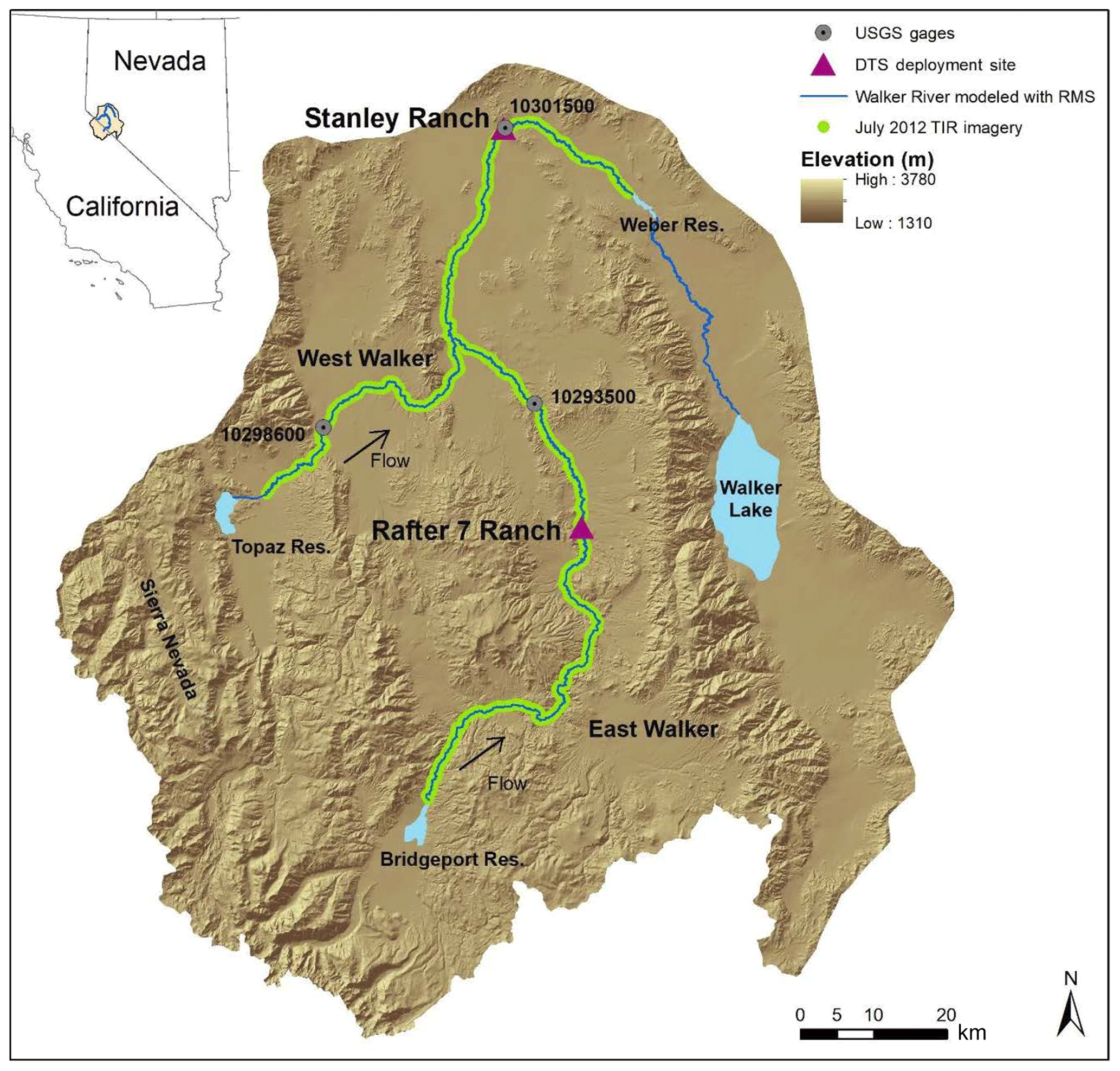
Figure 1 Walker River modeled extent, June 2015 DTS deployment sites, and July 2012 TIR imagery extent.

Agriculture is the main land use in the basin. Irrigated farmland makes up approximately 450 km² of the 10 720 km² Walker Basin (Sharpe et al., 2008). Bridgeport Reservoir on the East Walker River, Topaz Reservoir on the West Walker, and Weber Reservoir on the main stem Walker River regulate water to support agriculture and other human water uses. There are 23 diversions and 8 return flows in the East, West, and main stem Walker rivers, which influence both streamflows and stream temperatures. The Walker River generally gains water during wet years and loses flow during dry years (Carroll et al., 2010). Agricultural flood irrigation replenishes groundwater levels during the summer months (Carroll et al., 2010; Lopes and Allander, 2009).

Walker Lake once supported healthy populations of Lahontan cutthroat trout (LCT) (Oncorhynchus clarkii henshawi), which spawned in the Walker River and tributaries. The historic range of LCT is the Lahontan Basin in eastern California, southeastern Oregon, and northern Nevada, although LCT persist in less than 10 % of their historic range because they are limited by warm stream temperatures, low streamflows, and low dissolved oxygen (Coffin and Cowan, 1995; USFWS, 2003). LCT are now listed as a threatened species under the Endangered Species Act (USFWS, 1975). Field studies conducted in Coyote Lake (Oregon), Quinn River (Oregon and Nevada), and Humboldt River (Nevada) indicate LCT occurrence is reduced at stream temperatures above the acute (<2 h) threshold of 28 ^∘C (Dunham et al., 2003). Measured main stem Walker River stream temperatures exceeded the acute 28 ^∘C temperature threshold for LCT throughout summer in 2014 and 2015, demonstrating that warming stream temperatures are a concern for LCT in the Walker Basin (Null et al., 2017).

Low instream flows from surface water diversions have caused the Walker Lake level to decline, increasing dissolved salts in the lake to concentrations which do not support trout and native benthic insects (Herbst et al., 2013; Wurtsbaugh et al., 2017). To address these problems, an environmental water purchase program acquires natural flow and storage water rights from willing sellers who switch to crops that require less water or improve agricultural water use efficiency (NFWF, 2018; Walker Basin Conservancy, 2018). To date, 2.3 m³ s⁻¹ of natural flow water rights and 13.3 million m³ of storage water rights have been purchased, approximately 40 % of the water needed to restore Walker Lake salinity to tolerable levels (Walker Basin Conservancy, 2018). Previous modeling has suggested that environmental water purchases intended to increase lake elevation also improve habitat conditions for LCT and other aquatic biota in the Walker River by increasing streamflows, reducing stream temperatures, and increasing dissolved oxygen concentrations (Elmore et al., 2016; Null et al., 2017).

3 Methods

3.1 Distributed temperature sensing (DTS) data

3.1.1 DTS data collection

DTS units measure temperatures by sending a laser pulse down a fiber-optic cable and timing the return signal. Although most of the reflected energy has its original wavelength, a portion of the energy is absorbed and re-emitted at both shorter (anti-Stokes backscatter) and longer (Stokes backscatter) wavelengths. Temperatures along the cable are determined from the Stokes ∕ anti-Stokes ratio (Selker et al., 2006). A 1 km silver armored DTS cable was deployed to measure diurnal stream temperatures in the main stem and East Walker rivers. Data were collected over 400 m in the East Walker River at Rafter 7 Ranch on 18–23 June 2015 and over 450 m in the main stem Walker River at Stanley Ranch on 25–30 June 2015 (Fig. 1). The year 2015 was dry and the snowpack was at 5 % of normal levels. The DTS cable was deployed in a U shape at both sites, with approximately 400 m of cable on each side of the stream to capture lateral stream temperature differences. The cable was suspended in the water column approximately 10 cm above the streambed with steel stakes and leashes. Main stem Walker River DTS deployment included approximately 20 m of a flood irrigation return flow canal named the Wabuska Drain. The Wabuska Drain was not flowing during the drought when the DTS was deployed but contained standing water and was connected on the surface with the Walker River.

A two-channel Sensornet Orxy DTS unit measured stream temperatures at a spatial resolution of 1 m and temporal resolution of 15 min. Each data collection event measured temperatures over 30 s and averaged temperature over the 1 m spatial interval. Measurement precision from the unit was 0.01 ^∘C in the −40 to 65 ^∘C range. The DTS had two co-located fibers within the cable producing two single-ended datasets.

The DTS was dynamically calibrated during deployment with 10 m of cable placed in three recirculated calibration baths. One ambient and one ice bath were near the DTS unit and one ambient bath was at the end of the cable (Hausner et al., 2011; Tyler et al., 2009). RBRsolo thermocouple temperature sensors that are accurate to 0.002 ^∘C in the −5 to 35 ^∘C range measured calibration bath temperatures. Nine Maxim Integrated iButton thermistors provided additional stream temperature measurements along the cable every 15 min to verify DTS temperatures. iButton temperature loggers are accurate to 0.5 ^∘C in the −40 to 85 ^∘C range. Calibration used a linear transformation to correct the DTS data based on the difference between the DTS and thermocouple temperatures. Post-collection processing used the single-ended explicit calibration method developed by Hausner et al. (2011). Due to cable damage near the splice box prior to the third calibration bath, postprocessing relied upon iButton data closest to the end of the cable and the two calibration bath thermocouples near the DTS. Sections of cable that were exposed to air were removed from the dataset. Data points were also removed if the temperature difference between the two single-ended datasets was >1 ^∘C because tension on the DTS cable can result in erroneous temperature measurements (Hausner et al., 2011). Temperatures for these points were linearly interpolated between the upstream and downstream cable locations. We reported the average root mean square error (RMSE) of the two thermocouples and iButton to quantify DTS error for the length of the cable for each single-ended dataset. The single-ended dataset with the lowest calibrated RMSE was used for data analysis and results. In addition, RMSE was calculated between georeferenced iButton stream temperature measurements and the corresponding georeferenced DTS stream temperature measurements for the data collection period to provide additional corroboration of the DTS temperatures. iButton residuals were calculated as the difference between iButton temperatures and co-located DTS-measured temperatures.

A Decagon eKo Pro Series meteorological station with an eKO ET22 weather sensor collected solar radiation, wind speed and direction, air temperature, humidity, barometric pressure, and precipitation every 15 min at the DTS data collection locations for each deployment. Edge-of-water, DTS-cable-location, thalweg, and channel cross sections were surveyed with a Leica Viva GS14 GNSS Real Time Kinematic (RTK) GPS and measurements were accurate to approximately 2 cm in the x and y directions. USGS gages 10293500 and 10301500 provided flow data for the East Walker River and main stem Walker River, respectively. DTS deployments occurred on warm and clear summer days when maximum air temperatures were 34.7 ^∘C at the East Walker River and 37.9 ^∘C at the main stem Walker River DTS sites. Average flow was 1.2 m³ s⁻¹ (42 ft³ s⁻¹) in the East Walker River and 1.0 m³ s⁻¹ (36 ft³ s⁻¹) in the Walker River during deployment (Fig. S2).

3.1.2 DTS data analysis

DTS minimum ($T_{{\min }_{i,\mathrm{s}}}$), maximum ($T_{{\max }_{i,\mathrm{s}}}$), and site-averaged stream temperatures (${\stackrel{\mathrm{‾}}{T}}_{i,\mathrm{s}}$) were calculated for each DTS sample event, i, at each DTS site, s (Table 1). Similarly, minimum ($T_{{\min }_{\mathrm{p},\mathrm{s}}}$) and maximum ($T_{{\max }_{\mathrm{p},\mathrm{s}}}$) stream temperatures for the deployment period, p, at each DTS site were calculated. Deployment period average temperatures (${\stackrel{\mathrm{‾}}{T}}_{\mathrm{p},\mathrm{s}}$) were calculated from the spatial average of each sampling event, which occurred every 15 min, following Eq. (1):

$$\begin{array}{}\text{(1)}& {\stackrel{\mathrm{‾}}{T}}_{\mathrm{p},\mathrm{s}}={\displaystyle \frac{\sum _{i=\mathrm{1}}^t\left({\stackrel{\mathrm{‾}}{T}}_{i,\mathrm{s}}\right)}{p}}.\end{array}$$

Table 1 Description of DTS stream temperature variables.

The temperature range of each DTS sample event at a deployment site (R_i,s) was calculated by subtracting the minimum measured temperature ($T_{{\min }_{i,\mathrm{s}}}$) from the maximum measured temperature ($T_{{\max }_{i,\mathrm{s}}}$) for the 1000 m DTS cable. The minimum ($R_{{\min }_{\mathrm{p},\mathrm{s}}}$) and maximum ($R_{{\max }_{\mathrm{p},\mathrm{s}}}$) temperature range during the deployment period for each deployment site were also calculated. The deployment period average DTS stream temperature range (${\stackrel{\mathrm{‾}}{R}}_{\mathrm{p},\mathrm{s}}$) was calculated from the sample events for each DTS site following Eq. (2):

$$\begin{array}{}\text{(2)}& {\stackrel{\mathrm{‾}}{R}}_{\mathrm{p},\mathrm{s}}={\displaystyle \frac{\sum _{i=\mathrm{1}}^t\left(T_{{\max }_{i,\mathrm{s}}}{T}_{{\min }_{i,\mathrm{s}}}\right)}{p}}.\end{array}$$

Left and right river bank temperatures represent lateral thermal variability and were estimated from DTS data at 1, 10, 100, and 300 m extents to quantify thermal variability over multiple spatial scales. Lateral variability was evaluated for the hottest sample time during each DTS deployment in the main stem Walker and East Walker rivers. For the 1 m comparison, we used left and right bank measurements perpendicular to the thalweg. At larger spatial scales, we compared the minimum and maximum temperatures for each bank for 10, 100, and 300 m extents. The temperature range at each scale was then estimated as the maximum absolute value of the difference between the two banks. Wabuska Drain was not included in these analyses.

3.2 Airborne thermal infrared (TIR) data

3.2.1 TIR data collection

TIR imagery of the Walker River was collected by Watershed Sciences Inc. on 16–17 November 2011 (winter flight) and 18 and 24–26 July 2012 (summer flight) (Watershed Sciences Inc., 2011, 2012). We used summer TIR data for all analyses in this paper, except to identify possible cool-water seeps, which were more apparent with the winter dataset. The year 2012 was dry year and the snowpack was at 50 % of normal levels. TIR flights measured surface stream temperatures for 240 river kilometers in the East Walker, West Walker, and main stem Walker rivers to Weber Reservoir (Fig. 1). Stream temperatures warmed by 1 to 2 ^∘C (average 1.6 ^∘C) between 14:00 and 16:00 LT (local time) when TIR data were collected. A FLIR Systems, Inc. SC6000 sensor (wavelength of 8–9.2 µm, Noise Equivalent Temperature Differences of 0.035 ^∘C, and pixel array of 640×512 at a 14 bit encoding level) mounted on the underside of a Bell Jet Ranger Helicopter collected imagery and was flown at an altitude of approximately 610 m. Pixel resolution was 0.6 m (Watershed Sciences Inc., 2012).

Watershed Sciences Inc. calibrated and georeferenced the data and provided raster layers of the data. Tributary inflow temperatures were reported at their confluence with the Walker River. Watershed Sciences, Inc. also provided summary point data, which are minimum, median, and maximum temperatures of 10 pixels from the middle of the stream. Flight speed, image overlap, and river features determined which images to sample (Watershed Sciences Inc., 2012). We used georeferenced TIR rasters and summary points for analyses. TIR data were collected on warm summer days with low humidity. Average air temperature during data collection was 33.1 ^∘C and average wind speed was 11.6 km per hour (kph) in Yerrington, NV. Average flow during data collection was 1.0 m³ s⁻¹ (34 ft³ s⁻¹), 1.1 m³ s⁻¹ (39 ft³ s⁻¹), and 2.8 m³ s⁻¹ (100 ft³ s⁻¹) in the main stem Walker River (USGS gage 10301500), West Walker River (USGS gage 10298600), and East Walker River (USGS gage 10293500), respectively (Watershed Sciences Inc., 2012). Calibrated TIR radiant temperatures were validated with 28 Hobo Pro and iButton sensors. See Watershed Sciences Inc. (2012 and 2011) for additional TIR data collection details.

3.2.2 TIR data analysis

To compare measured TIR surface temperatures with model results, TIR summary points provided by Watershed Sciences Inc. (2012) were georeferenced with the 300 m modeled reaches. On average, there were three TIR summary points per 300 m modeled reach. The spatial averages of minimum, maximum, and median TIR temperature were calculated for the East Walker, West Walker, and main stem Walker rivers.

To evaluate TIR temperatures at multiple spatial scales, we clipped the TIR raster to the river channel, generated points at 50 and 300 m equal intervals along the river center line, buffered the points, and converted the layers to rasters. TIR pixels that included stream banks or vegetation were warmer than the river and skewed temperature range, average temperature, and maximum temperature zonal statistics. Thus, we compared zonal statistics for minimum pixel temperatures at the 50 and 300 m scales.

3.3 River Modeling System (RMS) modeled stream temperatures

Previous research provided modeled streamflows and stream temperatures for one wet (2011) and three dry (2012, 2014, 2015) 1 April–31 October irrigation seasons using River Modeling System (RMS) (Elmore et al., 2016; Null et al., 2017). RMS is a one-dimensional hydrodynamic and water quality model which solves the St. Venant equations for conservation of mass and momentum and the Holly–Priessmann mass transport equation (Hauser and Schohl, 2002). Input requirements for the hydrodynamics module are channel geometry, roughness coefficients, boundary condition streamflow, and initial surface water elevations. Outputs are velocity and depth at each model node which are passed to the water quality module. Additional inputs for the water quality module include weather data, riparian shading estimates, boundary temperatures, and initial water temperature. Water quality outputs are hourly stream temperatures (Hauser and Schohl, 2002).

The RMS model was developed to simulate stream temperatures from environmental water purchases that alter thermal mass. Irrigation season was modeled because it is the time period that environmental water purchases occur from irrigators. A total of 305 river kilometers were represented in RMS at an hourly time step. Model reaches over the model extent were 300 m. As a one-dimensional model, each reach was completely mixed and had a homogenous temperature. Walker River modeled extent included the East Walker River downstream of Bridgeport Reservoir (river kilometers 243 to 117), the West Walker River downstream of Topaz Reservoir (river kilometers 60 to 0) and the main stem Walker River to Walker Lake (river kilometers 117 to 0) (Fig. 1). For additional model details see Elmore et al. (2016) and Null et al. (2017).

3.4 Comparison of measured and modeled data

We calculated the percentage of time that the model over- or underpredicted DTS temperatures and the percentage of space that the model over- or underpredicted TIR temperatures to quantify the thermal range not captured within one-dimensional modeling. We used hourly, spatially averaged DTS measurements and omitted Wabuska Drain temperatures to compare DTS data to model results. TIR data were averaged for 300 m reaches to compare with model results. RMSE, mean absolute error (MAE), and mean bias summarized differences between modeled and measured data.

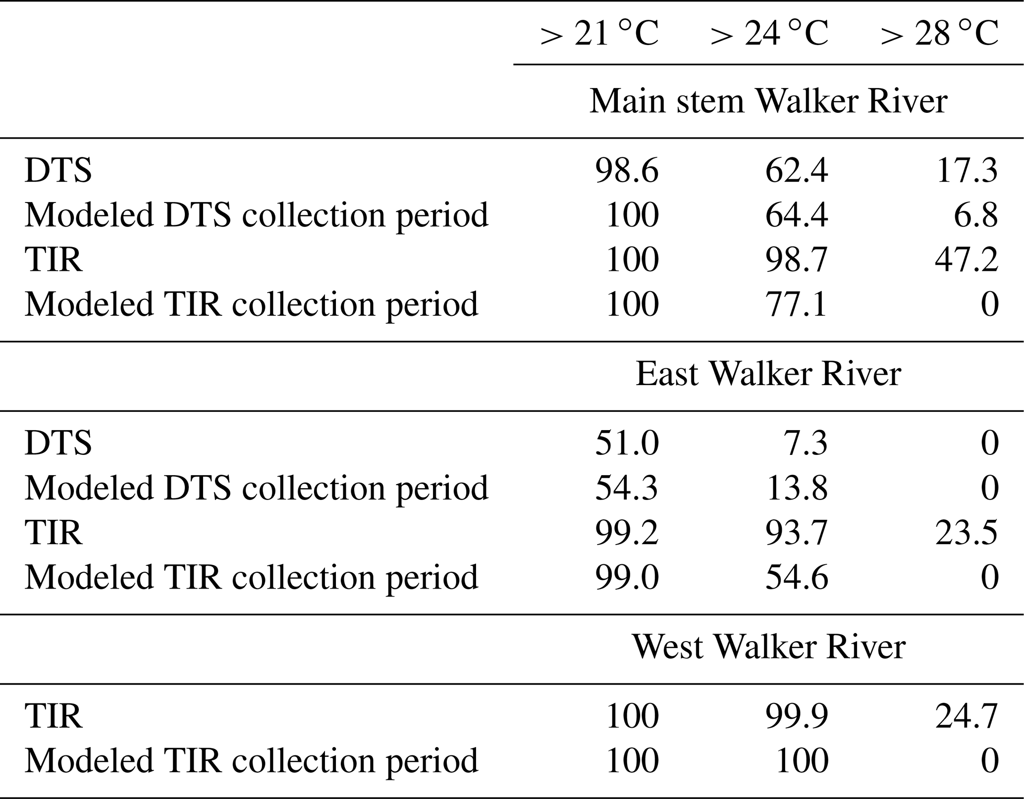
The percentage of time that DTS and modeled stream temperatures were below 21, 24, and 28 ^∘C and the river extent that TIR and modeled stream temperatures were below the same thresholds were also calculated. Temperatures below 21 ^∘C are optimal for adult LCT (Hickman and Raleigh, 1982), temperatures exceeding 24 ^∘C are stressful for LCT (Dickerson and Vinyard, 2003), and temperatures exceeding 28 ^∘C are lethal for LCT (Dunham et al., 2003).

Measured DTS and TIR temperature ranges for river features like return flows, diversions, beaver dams, and seeps provided estimates of small-spatial-scale thermal variability that may provide refugia for LCT and other cold-water species. To understand the influences of these features on temperatures throughout the basin, features were identified, georeferenced, and mapped to model reaches. Diversion and return flow locations were identified in 2012 by the Walker Basin Project (Tim Minor, personal communication, 2012). Seeps were identified during TIR surveys where stream temperatures varied from ambient river temperatures and temperature differences could not be attributed to shadows, cutbanks, or vegetation (Watershed Sciences Inc., 2011). We used seep locations identified during the winter TIR flight completed on 16–17 November 2011 because temperature differences were more obvious than the summer flight and some of the locations with groundwater seeps in the winter were dry during the summer flight (Watershed Sciences Inc., 2011, 2012). However, we quantified the observed temperature variability at seeps using the summer 2012 TIR flight (Watershed Sciences Inc., 2012). Beaver are native to the Walker Basin (Gibson and Olden, 2014) and beaver dams were identified using 2012 and 2013 Google Earth aerial imagery (Google Earth Pro, 2018). We included beaver dams that spanned the channel. Often turbulence was observed below the dam and sometimes crowdsourced photos added images of the beaver dams from the ground. We relied primarily on 2012 imagery, unless it was unavailable or of poor quality, when 2013 aerial imagery was used. Both 2012 and 2013 were dry years, and beaver dams are more abundant in the Walker River during dry years, when high flow events that limit beavers' ability to dam across the stream channel are reduced (Nevada Department of Wildlife, 2016). Using this information, we then added or subtracted measured temperature ranges to modeled temperatures at each of the georeferenced river features to provide an estimate of the thermal variability occurring at small spatial scales not captured by the one-dimensional model predictions.

4 Results

4.1 DTS stream temperatures and ranges

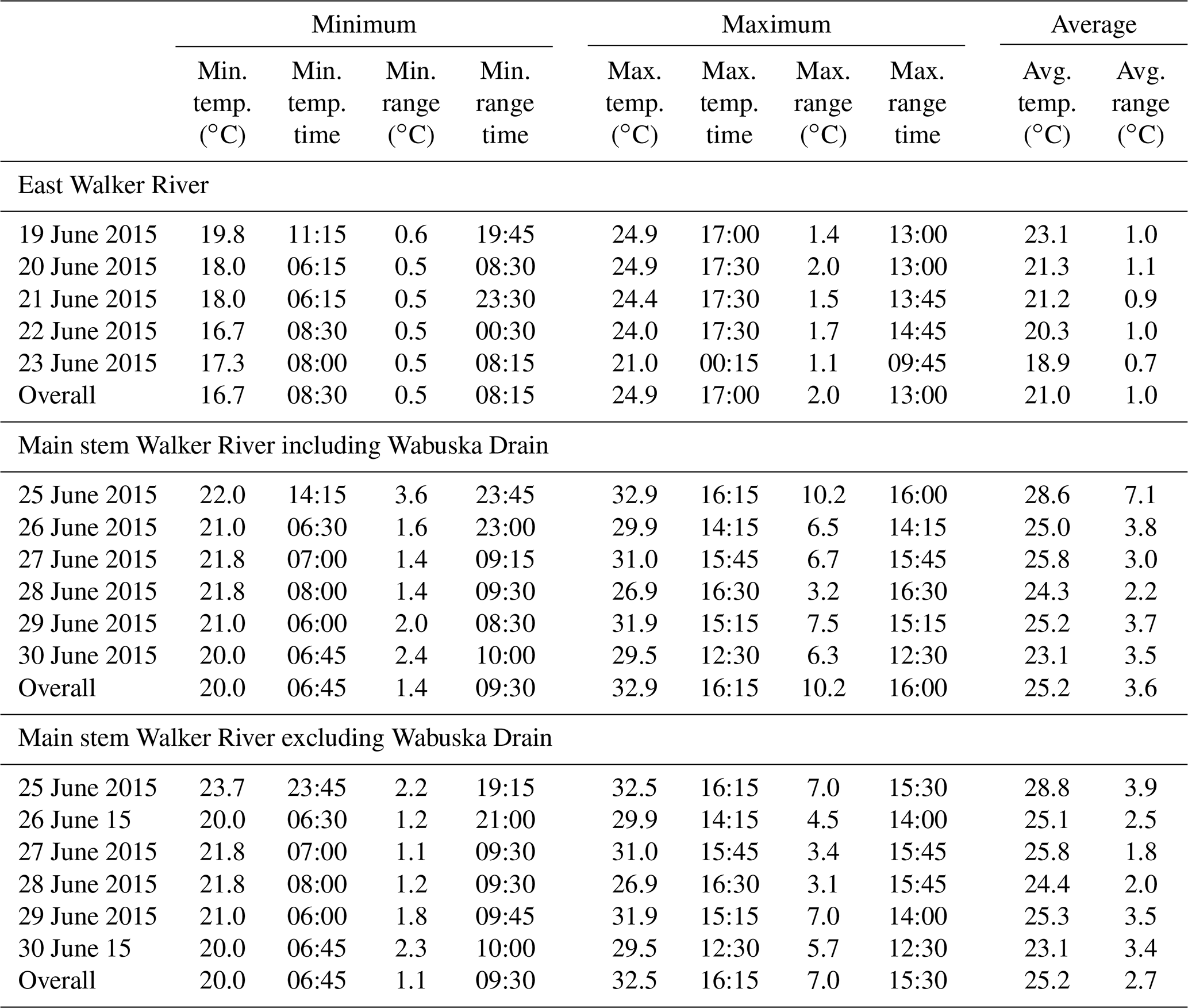
Average RMSE between calibrated DTS data and the three reference temperatures was 0.09 and 0.15 ^∘C for the East Walker River and main stem Walker River DTS sites, respectively (Table S1 in the Supplement). Average DTS error for both sites was also within the 0.5 ^∘C precision of the iButtons. There were no significant residual trends in errors for the main stem Walker River (Table S2 and Fig. S1 in the Supplement).

DTS temperatures in the East Walker River changed more through time than through space (Fig. 2). The deployment period minimum stream temperature ($T_{{\min }_{\mathrm{p},\mathrm{s}}}$) was 16.7 ^∘C, maximum temperature ($T_{{\max }_{\mathrm{p},\mathrm{s}}}$) was 24.9 ^∘C, and average stream temperature (${\stackrel{\mathrm{‾}}{T}}_{\mathrm{p},\mathrm{s}}$) was 21 ^∘C (Table 2). Maximum temperatures were measured in a straight, homogenous, unshaded section (Fig. 3). The stream temperature range for each DTS collection event (R_i,s) varied from a minimum of 0.5 ^∘C to a maximum of 2.0 ^∘C for the deployment period, with an average (${\stackrel{\mathrm{‾}}{R}}_{\mathrm{p},\mathrm{s}}$) of 1.0 ^∘C. A shaded backwater eddy and pools with overhanging shrubs and tall cottonwoods were river features with increased thermal heterogeneity in the East Walker River (Fig. 3).

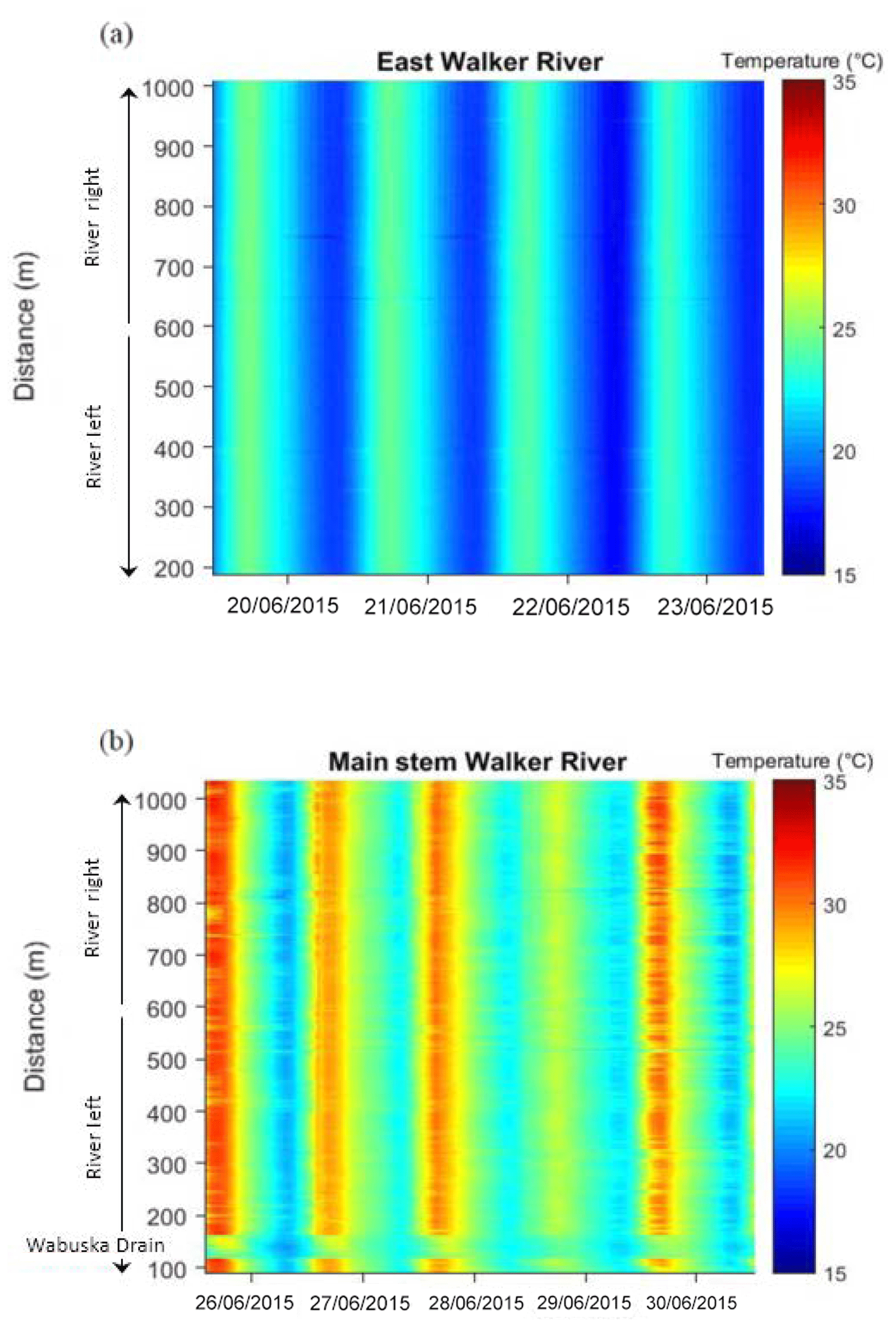
Figure 2 Stream temperatures measured for the length of the DTS cable at East Walker River (a) and main stem Walker River (b) DTS sites. Wabuska Drain, which was not flowing but had standing water during sampling, is located at cable distance 110–175 m in the main stem Walker River site.

Figure 3 East Walker River daily maximum stream temperatures on 21 June 2015. Insets show details of spatial temperature variability. Modeled reach points represent the division between 300 m modeled reaches.

Stream temperatures varied spatially throughout the main stem DTS site, visualized as color striations in Fig. 2b. Average deployment site temperature (${\stackrel{\mathrm{‾}}{T}}_{\mathrm{p},\mathrm{s}}$) was 25.2 ^∘C, not including the Wabuska Drain segment (Table 2, excluding distance 110–175 m in Fig. 2b). Maximum stream temperature ($T_{{\max }_{\mathrm{p},\mathrm{s}}}$) was 32.9 ^∘C. The average temperature range for the deployment (${\stackrel{\mathrm{‾}}{R}}_{\mathrm{p},\mathrm{s}}$) was 2.7 ^∘C, with a minimum deployment site temperature range ($R_{{\min }_{\mathrm{p},\mathrm{s}}}$) of 1.1 ^∘C and a maximum site temperature range ($R_{{\max }_{\mathrm{p},\mathrm{s}}}$) of 7.0 ^∘C. Average DTS stream temperatures (${\stackrel{\mathrm{‾}}{T}}_{\mathrm{p},\mathrm{s}}$) in the East Walker River were approximately 4 ^∘C cooler and less variable than the main stem Walker River (Fig. 2). Average DTS temperature ranges (${\stackrel{\mathrm{‾}}{R}}_{\mathrm{p},\mathrm{s}}$) were nearly 2 ^∘C greater in the main stem Walker River than the East Walker River. The East Walker River DTS site is farther upstream and close to Bridgeport Reservoir, a bottom release dam. The main stem Walker River DTS site is 92 km downstream from the East Walker River DTS site and receives contributions from the West Walker River, which is fed by surface water releases from Topaz Reservoir.

When the 20 m section of the Wabuska Drain return flow canal was analyzed with the main stem Walker River, daily minimum and maximum temperatures did not change because temperature variability across the deployment site was greater than localized variability in areas like the Wabuska Drain. However, the maximum temperature range during the deployment ($R_{{\max }_{\mathrm{p},\mathrm{s}}}$) increased considerably from 7.0 to 10.2 ^∘C and the average temperature range for the deployment (${\stackrel{\mathrm{‾}}{R}}_{\mathrm{p},\mathrm{s}}$) also increased from 2.7 to 3.6  ^∘C (Table 2, Fig. 2b). Figure 4 illustrates cooler temperatures in the Wabuska Drain during most times and spatial temperature variability during daily maximum stream temperatures on 29 July. The coolest temperature ($T_{{\min }_{i,\mathrm{s}}}$) at that time in the main stem Walker River DTS site was 24.4 ^∘C and occurred approximately 20 m into Wabuska Drain (Fig. 4). Stream temperatures of up to 31.8 ^∘C ($T_{{\max }_{i,\mathrm{s}}}$) occurred in the homogeneous main stem Walker River segment just upstream of the Wabuska Drain along the shallow right bank and at the mouth of the drain. The shallow Wabuska Drain also experienced rapid heating and cooling in response to atmospheric conditions. Cool water from the outlet of the Wabuska Drain mixed with the main stem Walker River at hot times of day, expanding the temperature range downstream of the drain. In addition to wider temperature ranges in the Wabuska Drain, the main stem Walker River had greater temperature heterogeneity from inactive, breached beaver dams. On 29 June at 15:15 LT, when average site temperature (${\stackrel{\mathrm{‾}}{T}}_{i,\mathrm{s}}$) was 29.6 ^∘C for this sample event, nearly 7 ^∘C of temperature range observed for this event occurred at a breached beaver dam (Fig. 4).

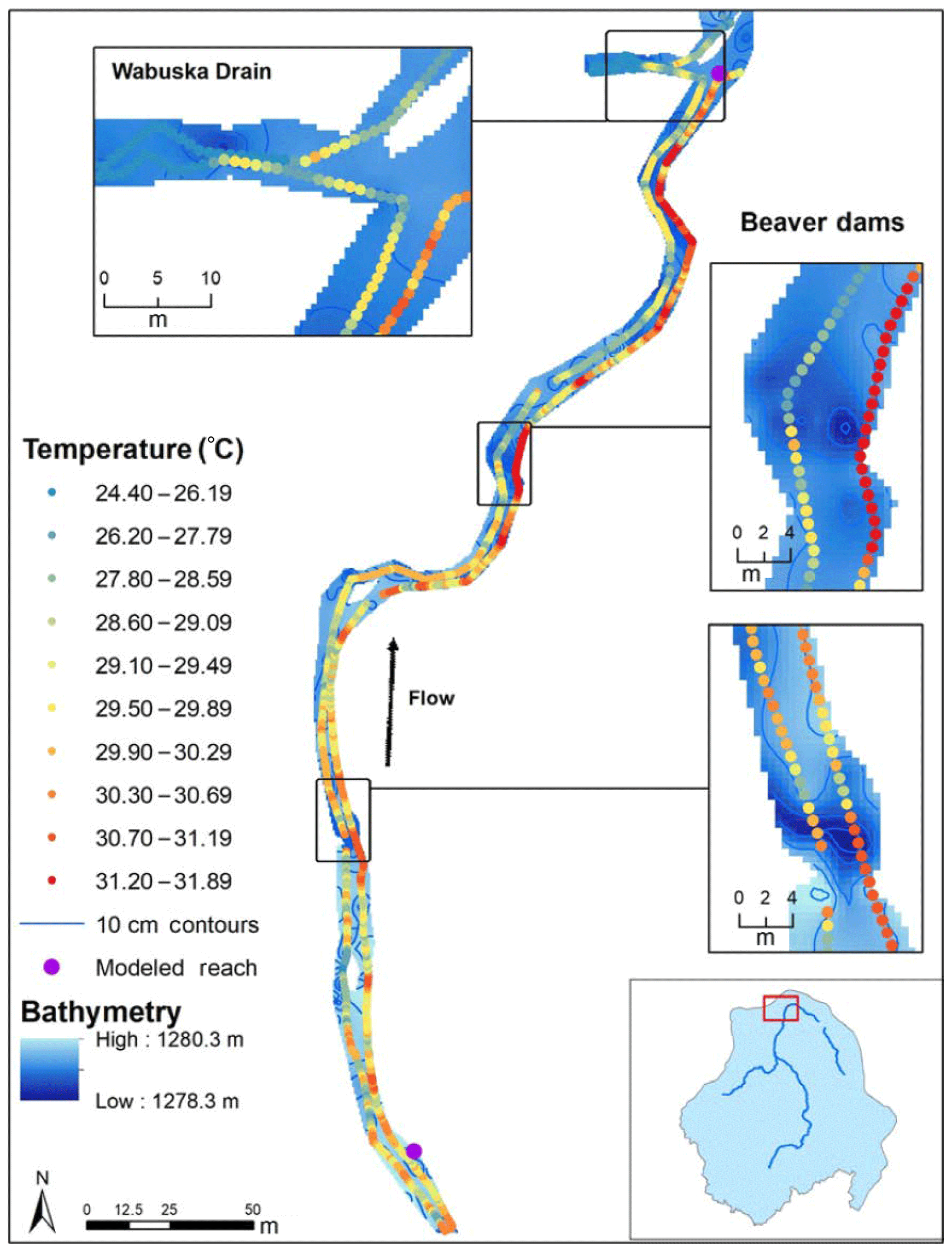
Figure 4 Main stem Walker River daily maximum stream temperature on 29 June 2015. Model reach points represent the division between 300 m model reaches.

Lateral DTS temperature variability was always greater in the main stem Walker River than the East Walker River. Temperature ranges increased as the spatial scale considered increased. The average lateral range was 0.2, 0.4, 0.7, and 0.9 ^∘C for 1, 10, 100, and 300 m spatial scales, respectively, in the East Walker River, and was 1.3, 2.7, 3.9, and 5.2 ^∘C for 1, 10, 100, and 300 m, respectively, in the main stem Walker River. These differences summarize the warmest temperature from one bank minus the coldest temperature from the other bank anywhere within the spatial scale considered. In the East Walker River site, deep pools and reaches with large wood structures were river features with distinctively lower temperatures than the rest of the river. In the main stem Walker River, deep pools with riparian vegetation, beaver dams, and islands in the channel were river features that were cooler or warmer than spatially averaged river temperatures.

Table 2 Daily stream temperatures and ranges for DTS deployments in the East Walker River (11:15 LT on 19 June 2015 to 09:45 LT on 23 June 2015) and main stem Walker River (14:15 LT on 25 June 2015 to 12:30 LT on 30 Jun 2019).

4.2 TIR stream temperatures and ranges

TIR data were within 0.5 ^∘C of iButton sensors, except for one location in the East Walker River where redundant sensors were 1.7 and 3.3 ^∘C cooler than radiant TIR temperature, and one location in the West Walker River where an iButton was 1.1 ^∘C cooler than radiant TIR temperature. TIR measures water surface temperatures, so these discrepancies may have occurred where the river was not well mixed.

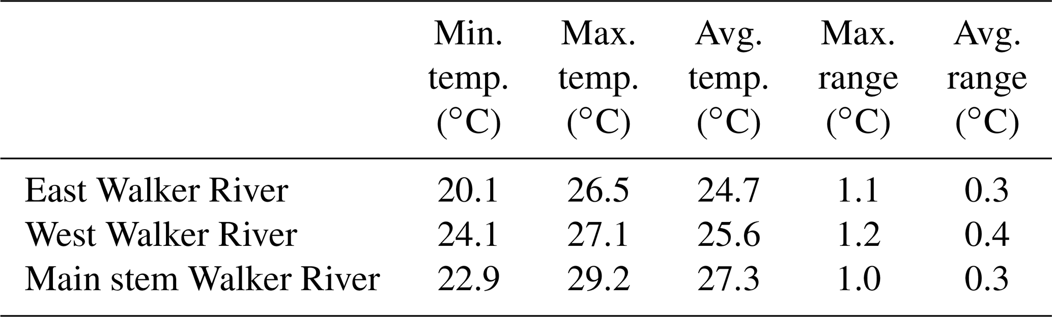
While DTS measurements provided high spatial and temporal stream temperature resolution at two sites, TIR measurements provided continuous stream surface temperatures throughout the Walker River for a single time. Maximum stream temperatures typically occurred in reaches with canal diversions and return flows. The warmest temperature in the East Walker River (Table 3) was 26.5 ^∘C where water ponds at a diversion (river kilometer 129). Maximum stream temperature in the West Walker River was 27.1 ^∘C and occurred upstream of the confluence with the main stem Walker River. Maximum temperature in the main stem Walker River was 29.2 ^∘C at the Wabuska Drain outflow (river kilometer 78). Although the Wabuska Drain received agricultural returns during the TIR flight and therefore contributed warm water, the 4.5 km stretch of river downstream from the Wabuska Drain was 1 ^∘C cooler than the river upstream of the Wabuska Drain (Fig. 5). This may be due to groundwater inflows downstream of the Wabuska Drain consistent with valley narrowing (Watershed Sciences Inc., 2012) or shallow groundwater contributions due to irrigation of adjacent fields. While groundwater interactions may have been less obvious when the return canal was flowing, DTS results showed evidence of cool water inputs when the canal was not flowing. Thus, monitoring suggests that large diversions and return flows can create warm water conditions when active, but they may also recharge shallow aquifers, increase shallow groundwater contributions, and create pockets of cold water. Shallow subsurface contributions to Wabuska Drain may not occur when groundwater levels decline outside of irrigation season (Naranjo and Smith, 2016).

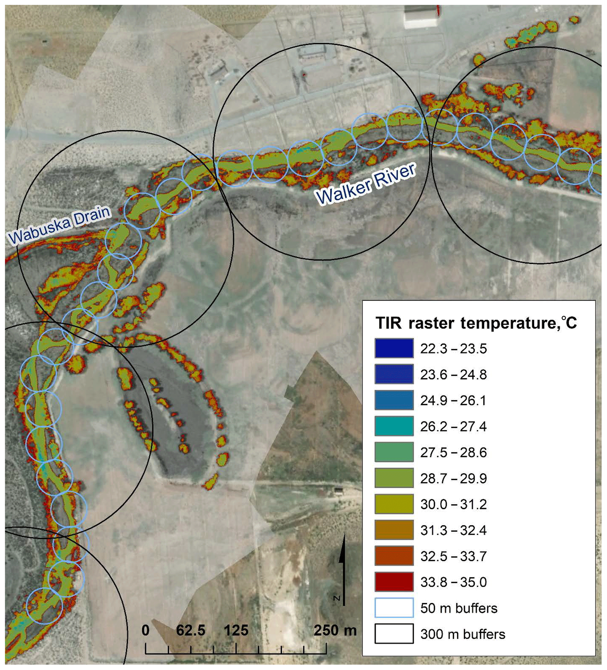
Figure 5 TIR raster data of the main stem Walker River near the Wabuska Drain with 50 and 300 m buffers.

Table 3 Stream temperatures and temperature range within 300 m modeled reaches by river from July 2012 TIR data.

The 300 m reaches with the greatest temperature ranges corresponded to locations of canal diversions, return flows, and groundwater seeps (Fig. 6). In the East Walker River, the Fox–Mickey Diversion (river kilometer 126) and Strosnider Diversion (river kilometer 140) had large temperature ranges. In the main stem Walker River, thermal variability occurred at the Spragg–Alcorn–Bewley Diversion (river kilometer 94), the Spragg–Alcorn–Bewley Canal Return (river kilometer 90), and Wabuska Drain (river kilometer 78) (Fig. 6). The maximum 300 m reach temperature range was 1.2 ^∘C in the West Walker River (river kilometer 58), which is the location of a groundwater seep (Watershed Sciences Inc., 2012). Thus, large diversions and return flows alter river depth and thermal mass while seeps increase temperature ranges by creating relatively consistent cool water. TIR data are unable to capture thermal stratification of beaver dams and ponds.

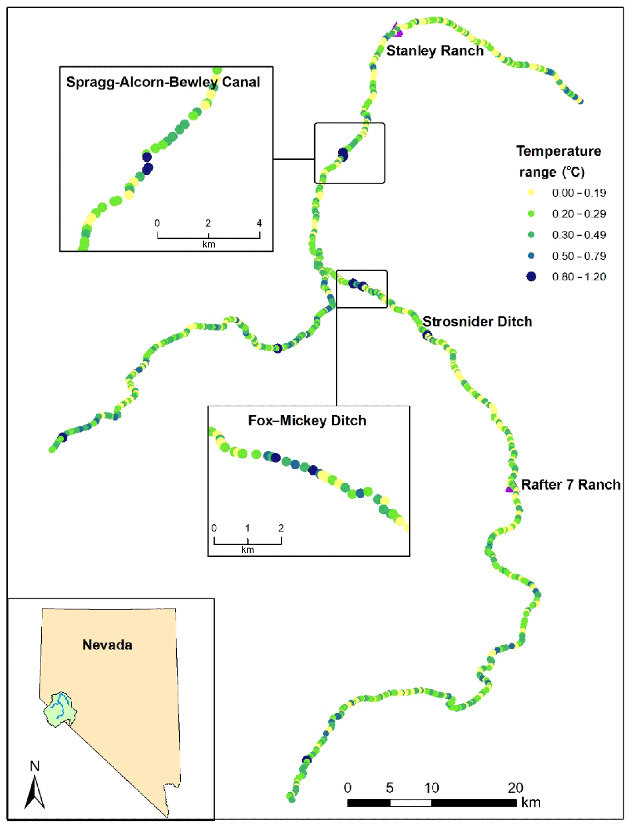
Figure 6 Temperature range within each 300 m model reach from July 2012 TIR summary point data.

Comparing minimum TIR stream temperatures at 50 and 300 m reaches improves understanding of thermal refugia at multiple spatial scales. We did not calculate temperature ranges because mixed pixels that contained water and land areas resulted in high maximum temperatures, and thus temperature ranges. We discuss this further in the limitations section. Overall, absolute minimum stream temperatures for each river were identical for 50 m and 300 m reaches, and were 21 ^∘C for the East and West Walker rivers and 22.3 ^∘C for the main stem Walker River. However, minimum temperatures varied among 50 m river segments that made up each 300 m river segment (Fig. 5). Thus, average minimum temperatures were 0.8 ^∘C warmer when analyzing data at the 50 m scale than the 300 m scale. This highlights the extent to which spatial temperature variability varies by the scale of analysis.

Table 4 RMSE, MAE, mean bias, and percent of modeled dataset outside of measured values for the East, West, and main stem Walker rivers between hourly modeled, DTS, and TIR stream temperatures.

4.3 RMS predictions vs. measured temperatures

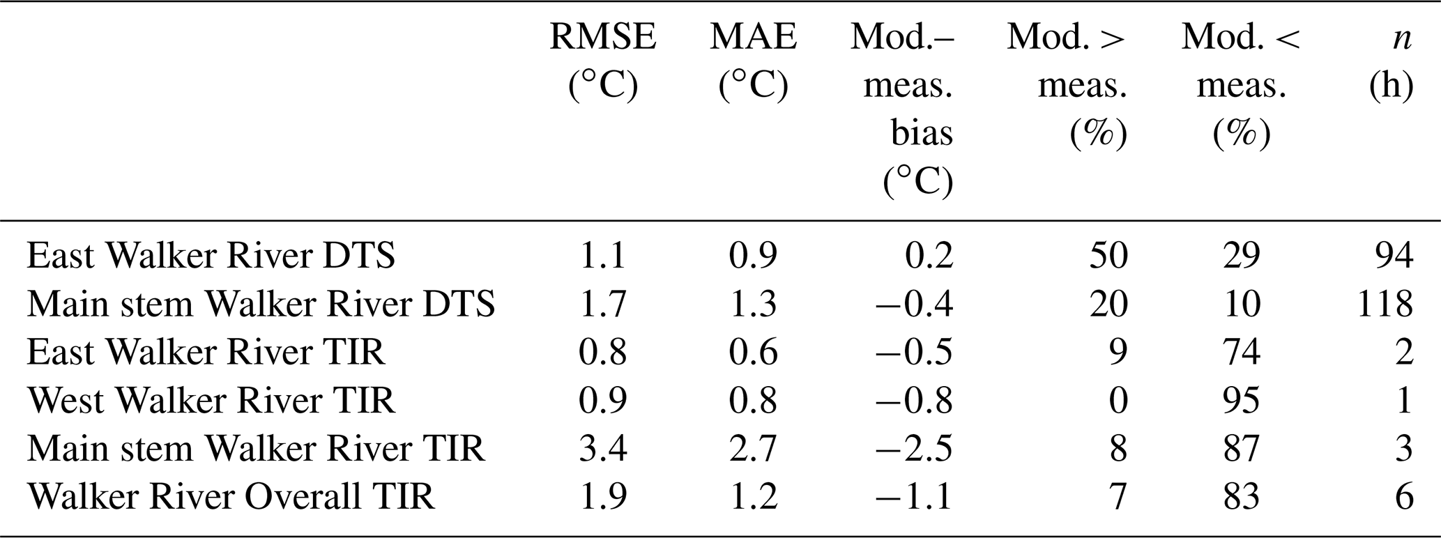
Modeled versus DTS stream temperature RMSE was 1.1 ^∘C in the East Walker River and 1.7 ^∘C in the main stem Walker River (Table 4). When compared to TIR data, RMSE and bias were both <1 ^∘C for the East and West Walker rivers. However, RMSE in the main stem Walker River was 3.4 ^∘C and bias was −2.5 ^∘C, where the model performed poorly under low flow conditions (Table 4). Main stem Walker River TIR versus modeled stream temperature was the only RMSE value that exceeded the calibrated RMS model RMSE of 2.5 ^∘C (Null et al., 2017). Model bias for the East Walker River indicated the model overestimated stream temperature by 0.2 ^∘C in the DTS site over the 5 d study period and underestimated temperature by 0.5 ^∘C for the 77 km TIR extent. In the main stem Walker River, the model underestimated stream temperatures by 0.4 ^∘C from the average DTS values and underestimated stream temperatures by 2.5 ^∘C when compared to the TIR data (Table 4).

Modeled temperatures in 2015 were warmer than DTS maximum hourly temperatures 50 % of the time in the East Walker River and 20 % of the time in the main stem Walker River. Conversely, the model underpredicted DTS temperatures 29 % and 10 % of the time in the East Walker and main stem Walker rivers, respectively (Table 4, Fig. 7a and b). Temperatures measured in Wabuska Drain were excluded from this analysis because the model simulated temperatures in the main channel only. Simulated 2012 temperatures were colder than TIR summary point minimum temperatures for 74 %, 95 %, and 87 % of survey extent in the East Walker, West Walker, and main stem Walker rivers, respectively (Fig. 7c–e, Table 4). Stream temperatures in the lower Walker River could be 4–6 ^∘C warmer than model predictions. That reach had challenging conditions for simulation models with a wide channel and low flow conditions.

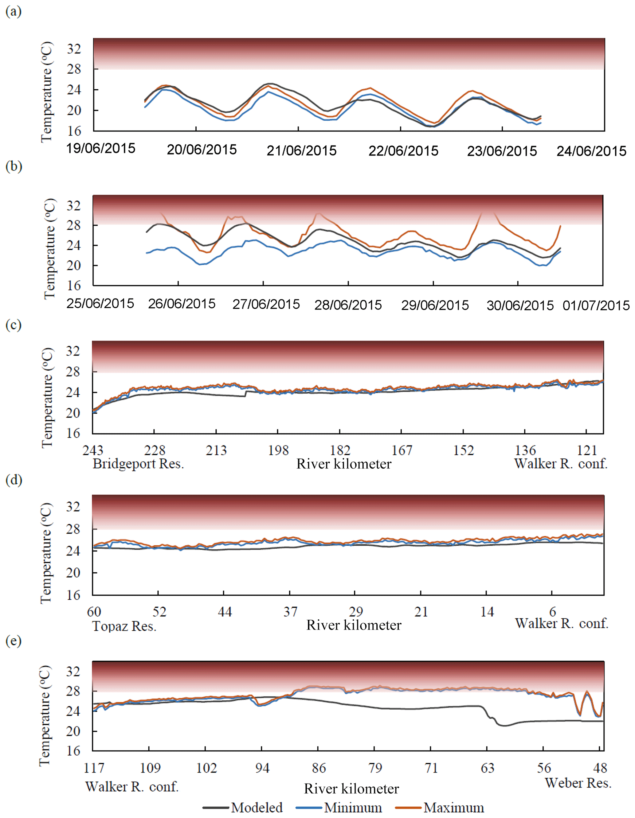
Figure 7 Hourly minimum and maximum DTS site temperatures compared to model predictions in the East Walker River (a) and main stem Walker River (b) (Wabuska Drain temperatures are not included as they were not modeled). July 2012 minimum and maximum TIR temperatures calculated for every 300 m model reach length compared to modeled temperatures for East Walker (c), West Walker (d), and main stem Walker (e) rivers. The upstream end of Weber Reservoir is river kilometer 48. The river flows from left to right in (c–e). Shaded region shows temperatures exceeding the 28 ^∘C lethal threshold for LCT.

4.4 Thermal habitat and thermal refugia connectivity

Stream temperatures were rarely cooler than 21 ^∘C, and this finding was consistent among the DTS, TIR, and modeled data (Table 5). An exception was during the East Walker River DTS deployment in June 2015, when nearly 50 % of DTS samples and modeled results were below 21 ^∘C. Of the TIR, DTS, and RMS model datasets evaluated, stream temperatures were most likely to exceed 28 ^∘C based on conditions captured in the TIR dataset. Nearly all TIR and modeled temperatures for the West Walker River were between 24 and 28 ^∘C in July 2012. However, with all datasets, the main stem Walker River nearly always exceeded 21 ^∘C, usually exceeded 24 ^∘C, and could exceed 28 ^∘C. TIR stream temperature measurements in the lower reaches of the main stem Walker River remained near the LCT lethal temperature threshold for an additional 45 km than was previously estimated using the temperature model.

Table 5 Percentage of DTS, TIR, and RMS model stream temperatures that exceed 21, 24, and 28 ^∘C temperature thresholds.

Measured DTS and TIR temperature ranges from return flows, diversions, beaver dams, and seeps were added or subtracted to perfectly mixed 300 m modeled reach stream temperatures to estimate thermal refugia connectivity. We identified 23 diversions, 8 return flows, 53 possible seeps, and 42 beaver dams throughout the modeled reach (Fig. 8a). We used average temperature changes of −2.5 ^∘C for return flows, +1.2 ^∘C for diversions, −3.2 ^∘C for beaver dams, and −1.9 for groundwater seeps, although observed temperature variability for each feature showed differences from ambient river temperatures varied from −10.1 to +2.3 ^∘C for return flows, −1.2 to +4 ^∘C for diversions, −5.1 to +2 ^∘C for beaver dams, and −4.2 to 0 ^∘C for seeps. Adding observed DTS and TIR temperature variability to model results indicates that cool-water refugia may sometimes exist to support species migration between Walker Lake and tributaries of the Walker River (Fig. 8b). The shortest distance between refugia, or cooler pockets of water, was 0.3 km, which was the spatial resolution of model reaches. The maximum distance between refugia was 37 km and occurred near Weber Reservoir in the main stem Walker River. The mean distance between refugia was 2.8 km and the median distance was 0.9 km.

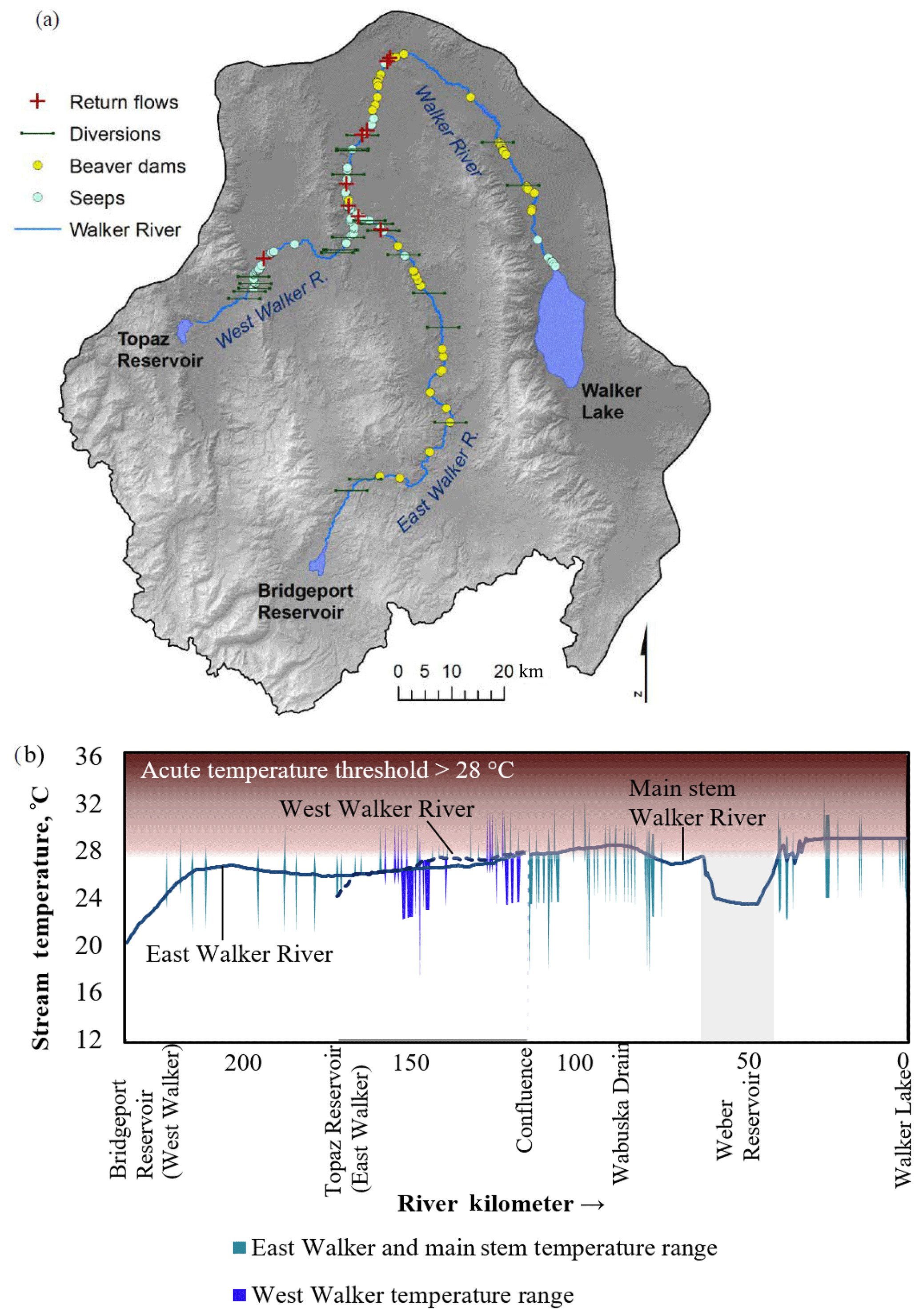
Figure 8 Locations of river features that affect stream temperatures in the Walker Basin (a). Daily maximum RMS stream temperatures for 29 June 2015 with estimated temperature variability by river feature using daily maximum DTS data from 29 June 2015 and TIR data from 2012 (b).

5 Limitations

DTS data collection limitations include cable drift, stress, and solar heating, which have been previously described in the literature (Tyler et al., 2009). In our deployments, solar heating of the DTS cable was assumed to be negligible because the cable was silver coated (Tyler et al., 2009) and solar heating of DTS cables would be limited due the reflective coating combined with the advection-dominated and turbid conditions present within most of the Walker River (Neilson et al., 2010). Field crews used leashes to secure the DTS cable, which was monitored daily to minimize stress and drift. We deployed the DTS during mid-summer when we anticipated stream temperatures would be warm as a worst-case scenario for thermal habitat. Additional research is needed to quantify how results would change when the Wabuska Drain is flowing, or for deployments earlier or later in summer.

TIR measures surface water temperatures, which may overestimate water column temperatures from vertical stratification and thermal boundary layer effects (Torgersen et al., 2001). Surface roughness, surface emissivity, surface reflection, variable background temperatures (e.g., sky versus trees), turbidity, changes in viewing aspect, aircraft type, flight speed, wind gusts, and length of time required to collect data all affect TIR image and data quality (Dugdale, 2016). Clipping TIR data to the stream channel was imprecise for datasets collected over large spatial extents. If pixels included stream banks or vegetation, they skewed calculations. For this reason, we did not report maximum temperatures of pixels within 50 or 300 m reaches, nor could we report temperature ranges which relied upon maximum temperature pixels. We assumed a vertically mixed water column when analyzing the DTS and TIR data. Pools and beaver dams may stratify vertically, increasing the local temperature variability from what was measured or predicted. Quantifying temperature range from vertical stratification was outside the scope of this paper.

Obtaining small-scale spatial and temporal stream temperatures and comparing them to model results has several limitations. First, resolution varied between DTS, TIR, and modeled data, reducing the number of comparable observations. TIR imagery represents a single point in time unless flights are repeated. DTS measurements were dense (1 m in these deployments with a 15 min temporal resolution) but were limited by cable length and field crews to monitor the deployment. Second, DTS and TIR measurements were collected in different years because we used existing TIR imagery collected as part of the Walker Basin Project, a multipartner effort to sustain the basin's economy, ecosystem, and lake. Future studies could collect data specifically to overlap in time and space so that temperature distributions along the river are not affected by different years and sample periods. However, opportunistically using existing data for reanalysis and to improve model result interpretation and river management is a laudable goal that may reduce the cost of river science and management. Multiyear and multipartner river monitoring, modeling, and management is common in large, important, or complex river basins. This research highlights the differences in temperature variability given alternative sampling and modeling methods.

6 Discussion

We measured small-scale stream temperature variability that was unquantified in an existing one-dimensional, basin-scale model. Overall, DTS measured a larger maximum temperature range than TIR imagery in the East Walker River (2.0 and 1.1 ^∘C, respectively) and main stem Walker River (10.2 and 1.0 ^∘C, respectively) (Tables 2 and 3) because DTS could measure temperatures that varied spatially within the water column and over short distances where beaver dams or return flows existed. The warmest temperatures were measured by TIR in the East Walker River (26.5 ^∘C), but by DTS in the main stem Walker River (32.9 ^∘C), indicating that these methods complement each other, but also suggesting that different years may result in alternate temperature distributions along the river (Tables 2 and 3). DTS and TIR augment process-based modeling by identifying river features that may provide thermal refugia. The range of temperatures in river features like seeps, beaver dams, diversions, and return flows were added to simulated temperatures to estimate thermal refuge distribution throughout the watershed. Coupling high-resolution stream temperature monitoring with process-based modeling results in a more realistic stream temperature range than one-dimensional modeling alone, especially when model results assess habitat suitability to identify promising restoration strategies and watershed-scale management.

Temperature ranges reported here are comparable to those previously reported in the literature. Cristea and Burges (2009) observed 2–3 ^∘C temperature differences downstream of cold-water seeps in the Pacific Northwest, which is similar to the 1–2 ^∘C temperature variability observed in the East Walker River in the DTS data and TIR imagery. Beaver dams had especially high temperature variability, consistent with findings from Majerova et al. (2015) and Weber et al. (2017). A 7 ^∘C temperature range was observed within a beaver dam in the main stem Walker River during a DTS sampling event. Fine spatial and temporal resolution stream temperature monitoring, paired with watershed-scale modeling, indicates that the distance between refugia varied from 0.3 to 37 km in the Walker River, closer together than the 5.7 to 49.4 km demonstrated by Fullerton et al. (2018) in the Pacific Northwest.

Thermal refugia are likely needed for species to persist near the margins of their distributions (Brewitt and Danner, 2014). Previous research has shown that the main stem Walker River has low streamflows and warm stream temperatures that do not support LCT or other cold-water species, but that the East and West Walker rivers are likely to support native aquatic species (Elmore et al., 2016; Hogle et al., 2014; Mehler et al., 2015; Null et al., 2017). This research nuanced those findings by highlighting the distribution and temperature ranges of likely thermal refugia in the main stem Walker River. Although detailed movement and summer home range data are unavailable for LCT, movement patterns have been described for Bonneville cutthroat trout (Schrank and Rahel, 2004) and Colorado River cutthroat trout (Young, 1996). Bonneville cutthroat trout move up to 82 km between spawning and over-summer habitats, with farther movements positively correlated to fish length (Schrank and Rahel, 2004). However, movement declines through summer. The median summer home range of Colorado River cutthroat trout is 0.2 km (Young, 2004) and Bonneville cutthroat trout typically do not move more than 0.5 km during summer (Schrank and Rahel, 2004). This suggests that the existing network of thermal refugia in the main stem Walker River may be adequate for LCT to move between spawning and lake habitats (following lake restoration) but is unlikely to provide refugia necessary for summer habitat. If native fish have not migrated through warm reaches by summer, they must shelter in refuges to thermoregulate body temperature (Frechette et al., 2018) and nearby foraging habitat would be needed to maintain body temperatures (Pépino et al., 2015). Understanding aquatic habitat availability and thermal refugia connectivity in the Walker Basin could reduce the need for large-scale river management decision-making that evaluates instream versus offstream water uses (Génova et al., 2018).

From a broader perspective, coupling high-resolution DTS and TIR measurements with process-based modeling contributes to literature describing thermal refugia networks (Isaak et al., 2012; Sutton et al., 2007). River features like diversions, return flows, and beaver dams provide temperature variability and often thermal refugia for cold-water species. However, trout use of thermal refugia may vary, as availability of thermal refugia changes with streamflow and weather conditions, and as trout habitat needs vary with life stage (Frechette et al., 2018; Dugdale et al., 2013). Additional work is needed to understand the resiliency of streamflows and thermal refugia with interannual variability and with anticipated climate change (McCullough et al., 2009; Ficklin et al., 2018; Null and Prudencio, 2016). Combining temperature modeling with small-scale stream temperature measurements upscales monitoring results and leverages existing modeling to improve understanding of small-scale temperature variability. This approach could be used by researchers and stakeholders who wish to improve interpretation of model results with observations to reduce the cost of river science and management.