Performance of bias-correction schemes for CMORPH rainfall estimates in the Zambezi River basin

Satellite rainfall estimates (SREs) are prone to bias as they are indirect derivatives of the visible, infrared, and/or microwave cloud properties, and hence SREs need correction. We evaluate the influence of elevation and distance from large-scale open water bodies on bias for Climate Prediction Center-MORPHing (CMORPH) rainfall estimates in the Zambezi basin. The effectiveness of five linear/non-linear and time–space-variant/-invariant bias-correction schemes was evaluated for daily rainfall estimates and climatic seasonality. The schemes used are spatio-temporal bias (STB), elevation zone bias (EZ), power transform (PT), distribution transformation (DT), and quantile mapping based on an empirical distribution (QME). We used daily time series (1998–2013) from 60 gauge stations and CMORPH SREs for the Zambezi basin. To evaluate the effectiveness of the bias-correction schemes spatial and temporal cross-validation was applied based on eight stations and on the 1998–1999 CMORPH time series, respectively. For correction, STB and EZ schemes proved to be more effective in removing bias. STB improved the correlation coefficient and Nash–Sutcliffe efficiency by 50 % and 53 %, respectively, and reduced the root mean squared difference and relative bias by 25 % and 33 %, respectively. Paired t tests showed that there is no significant difference (p < 0.05) in the daily means of CMORPH against gauge rainfall after bias correction. ANOVA post hoc tests revealed that the STB and EZ bias-correction schemes are preferable. Bias is highest for very light rainfall (< 2.5 mm d⁻¹), for which most effective bias reduction is shown, in particular for the wet season. Similar findings are shown through quantile–quantile (q–q) plots. The spatial cross-validation approach revealed that most bias-correction schemes removed bias by > 28 %. The temporal cross-validation approach showed effectiveness of the bias-correction schemes. Taylor diagrams show that station elevation has an influence on CMORPH performance. Effects of distance > 10 km from large-scale open water bodies are minimal, whereas effects at shorter distances are indicated but are not conclusive for a lack of rain gauges. Findings of this study show the importance of applying bias correction to SREs.

1 Introduction

Correction schemes for rainfall estimates are developed for climate models (Maraun, 2016; Grillakis et al., 2017; Switanek et al., 2017), for radar approaches (Cecinati et al., 2017; Yoo et al., 2014), and for satellite-based, multi-sensor approaches (Najmaddin et al., 2017; Valdés-Pineda et al., 2016). In this study the focus is on satellite rainfall estimates (SREs) to improve reliability in spatio-temporal rainfall representation.

Studies in satellite-based rainfall estimation show that estimates are prone to systematic and random errors (Gebregiorgis et al., 2012; Habib et al., 2014; Shrestha, 2011; Tesfagiorgis et al., 2011; Vernimmen et al., 2012; Woody et al., 2014). Errors result primarily from the indirect estimation of rainfall from visible (VIS)-, infrared (IR)-, and/or microwave (MW)-based satellite remote sensing of cloud properties (Pereira Filho et al., 2010; Romano et al., 2017). Systematic errors in SREs commonly are referred to as bias, which is a measure that indicates the accumulated difference between rain-gauge observations and SREs. Bias in SREs is expressed for rainfall depth (Habib et al., 2012b), rain rate (Haile et al., 2013), and frequency at which rain rates occur (Khan et al., 2014). Bias may be negative or positive, where negative bias indicates underestimation, whereas positive bias indicates overestimation (Liu, 2015; Moazami et al., 2013).

Recent studies on the National Oceanic and Atmospheric Administration (NOAA) Climate Prediction Center-MORPHing (CMORPH) (Wehbe et al., 2017; Jiang et al., 2016; Liu et al., 2015; Haile et al., 2015) reveal that the accuracy of this satellite rainfall product varies across regions (Gumindoga et al., 2019), but causes are not directly identifiable. As such correction schemes serve to reduce systematic errors and to improve applicability of SREs. Correction schemes rely on assumptions that adjust errors in space and/or time (Habib et al., 2014). Some correction schemes consider correction only for spatially distributed patterns in bias, commonly known as space-variant/-invariant. Approaches that correct for spatially averaged bias have roots in radar rainfall estimation (Seo et al., 1999), but are unsuitable for large-scale basins (> 5000 km²) where rainfall may substantially vary in space (Habib et al., 2014). Studies by Müller and Thompson (2013) in Nepal concluded that space-variant correction schemes are more effective in reducing bias for CMORPH and TRMM than space-invariant correction schemes. In a study conducted in the Upper Blue Nile basin in Ethiopia, Bhatti et al. (2016) show that CMORPH bias correction is most effective when bias factors are calculated for 7 d sequential windows.

Bias-correction schemes based on regression techniques have reported distortion of frequency of rainfall rates (Ines and Hansen, 2006; Marcos et al., 2018). Multiplicative shift procedures tend to adjust SRE rainfall rates, but Ines and Hansen (2006) reported that they do not correct systematic errors in rainfall frequency of climate models. Non-multiplicative bias-correction schemes preserve the timing of rainfall within a season (Fang et al., 2015; Hempel et al., 2013). Studies that have applied non-linear bias-correction schemes such as power functions report correction of extreme values (depth, rate, and frequency), thus mitigating the underestimation and overestimation of CMORPH rainfall (Vernimmen et al., 2012). The study by Tian (2010) in the United States noted that the Bayesian (likelihood) analysis techniques are found to over-adjust both light and heavy CMORPH rainfall.

Bias often exhibits a topographic and latitudinal dependency as, for instance, shown for the CMORPH product in the Nile basin (Bitew et al., 2011; Habib et al., 2012a; Haile et al., 2013). For southern Africa, Thorne et al. (2001), Dinku et al. (2008), and Meyer et al. (2017) show that bias in rainfall rate and frequency can be related to location, topography, local climate, and season. The first studies in the Zambezi basin (southern Africa) on SREs show evidence that necessitates correction of SREs. For example, Cohen Liechti (2012) show bias in CMORPH SREs for daily rainfall and for accumulated rainfall at a monthly scale. Matos et al. (2013), Thiemig et al. (2012), and Toté et al. (2015) show that bias in rainfall depth at time intervals ranging from daily to monthly varies across geographical domains in the Zambezi basin and may be as large as ±50 %. Besides elevation, there are indications that the presence of a large-scale open water body affects rainfall at short distances (< 10 km) (Haile et al., 2009).

For less developed areas such as in the Zambezi basin that is selected for this study, studies on SREs are limited. This is despite the strategic importance of the basin in providing water to over 30 million people (World Bank, 2010a). An exception is the study by Beyer et al. (2014) on correction of the TRMM-3B42 product for agricultural purposes in the Upper Zambezi basin. Studies (Cohen Liechti et al., 2012; Meier et al., 2011) on use of SREs in the Zambezi River basin mainly focused on accuracy assessment of the SREs using standard statistical indicators, with little or no effort to perform bias correction despite the evidence of errors in these products. The use of uncorrected SREs is reported for hydrological modelling in the Nile basin (Bitew and Gebremichael, 2011) and Zambezi basin (Cohen Liechti et al., 2012), respectively, and for drought monitoring in Mozambique (Toté et al., 2015). The poor performance of SREs in the above studies urges bias correction to result in more accurate rainfall representation. The selection of CMORPH satellite rainfall for this study is based on successful applications of bias-corrected CMORPH estimates in African basins for hydrological modelling (Habib et al., 2014) and flood predictions in western Africa (Thiemig et al., 2013). In the first publications on CMORPH, Joyce et al. (2004) describe CMORPH as a gridded precipitation product that estimates rainfall with information derived from IR data and MW data. CMORPH combines the retrieval accuracy of passive MW estimates with IR measurements which are available at high temporal resolution but with low accuracy. The important distinction between CMORPH and other merging methods is that the IR data are not used for rainfall estimation, but are used only to propagate rainfall features that have been derived from microwave data. The flexible “morphing” technique is applied to modify the shape and rate of rainfall patterns. CMORPH has been operational since 2002, for which data are available at the CPC of the National Centers for Environmental Prediction (NCEP) (after http://www.ncep.noaa.gov/, last access: 4 July 2019). Recent publications on CMORPH in African basins exist (Wehbe et al., 2017; Koutsouris et al., 2016; Jiang et al., 2016; Haile et al., 2015). However, studies on bias correction of CMORPH in the semi-arid Zambezi basin are limited.

In this study we use daily CMORPH and rain-gauge data for the Upper, Middle, and Lower Zambezi basins to (1) evaluate whether performance of CMORPH rainfall is affected by elevation and distance from large-scale open water bodies, (2) evaluate the effectiveness of linear/non-linear and time–space-variant/-invariant bias-correction schemes, and (3) assess the performance of bias-correction schemes to represent different rainfall rates and climate seasonality. Analysis serves to improve reliability of SREs applications in water resource applications in the Zambezi basin such as for rainfall–runoff modelling.

2 Study area

The Zambezi River is the fourth-longest river (∼2574 km) in Africa, with a basin area of ∼1 390 000 km² (∼4 % of the African continent). The river drains into the Indian Ocean and has a mean annual discharge of 4134 m³ s⁻¹ (World Bank, 2010a). The river has its source in Zambia with basin boundaries in Angola, Namibia, Botswana, Zambia, Zimbabwe, and Mozambique (Fig. 1). The basin is characterised by considerable differences in elevation and topography, distinct climatic seasons, and the presence of large-scale open water bodies and, as such, makes the basin well suited for this study. The basin is divided into three sub-basins, i.e. the Lower Zambezi comprising the Tete, Lake Malawi/Shire, and Zambezi Delta basins, the Middle Zambezi comprising the Kariba, Mupata, Kafue, and Luangwa basins, and the Upper Zambezi comprising the Kabompo, Lungwebungo, Luanginga, Barotse, and Cuando/Chobe basins (Beilfuss, 2012).

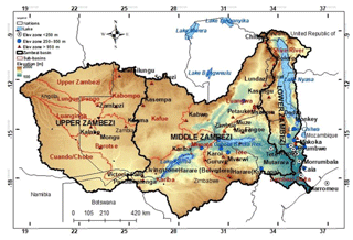
Figure 1 Zambezi River basin from Africa with sub-basins, major lakes, elevation, and locations and names of the 60 rain-gauging stations (in each respective elevation zone) used in this study.

The elevation of the Zambezi basin ranges from < 200 m (for some parts of Mozambique) to > 1500 m above sea level (for some parts of Zambia). Large-scale open water bodies in and around the basin are Kariba, Cabora Bassa, Bangweulu, Chilwa, and Nyasa. The Indian Ocean lies to the east of Mozambique. Typical land-cover types are woodland, grassland, water surfaces, and cropland (Beilfuss et al., 2000). The basin lies in the tropics between 10 and 20^∘ S, encompassing humid, semi-arid, and arid regions dominated by seasonal rainfall patterns associated with the Inter-Tropical Convergence Zone (ITCZ), a convective front oscillating along the Equator (Cohen Liechti et al., 2012). The movement of the ITCZ in the Southern Hemisphere results in the peak rainy season that occurs during the summer (October to April) and the dry winter months (May to September), and is a result of the shifting back of the ITCZ towards the Equator (Schlosser and Strzepek, 2015). The weather system in south-eastern parts such as Mozambique is dominated by Antarctic polar front (APF) and tropical temperate trough (TTT) occurrence which is positively related to La Niña and Southern Hemisphere planetary waves, whereas El Niño–Southern Oscillation (ENSO) appears to play a significant role in causing dry conditions in the basin (Beilfuss, 2012).

The basin is characterised by high annual rainfall (> 1400 mm yr⁻¹) in the northern and north-eastern areas and by low annual rainfall (< 500 mm yr⁻¹) in the southern and western parts (World Bank, 2010b). Due to this rainfall distribution, northern tributaries in the Upper Zambezi sub-basin contribute 60 % of the mean annual discharge (Tumbare, 2000). The river and its tributaries are subject to seasonal floods and droughts that have devastating effects on the people and economies of the region, especially the poorest members of the population (Tumbare, 2005). It is not uncommon to experience both floods and droughts within the same hydrological year.

3 Materials and methodology

3.1 Rainfall data

3.1.1 CMORPH

For this study, time series of CMORPH rainfall images (1998–2013) at 8 km ×8 km, 30 min resolution were selected and downloaded from the NOAA repository (ftp://ftp.cpc.ncep.noaa.gov/precip/global_CMORPH/, last access: 4 July 2019). Images are downloaded by means of the GeoNETCAST ISOD toolbox of the ILWIS GIS software (http://52north.org/downloads/, last access: 4 July 2019). Half-hourly estimates were aggregated to daily totals to match the observation interval of gauge-based daily rainfall.

3.1.2 Rain-gauge network

Time series of daily rainfall from 60 stations were obtained from meteorological departments in Botswana, Malawi, Mozambique, Zambia, and Zimbabwe for stations that cover the study area. All the stations are standard-type rain gauges with a measuring cylinder whose unit of measurement is millimetres (mm).

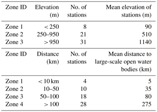
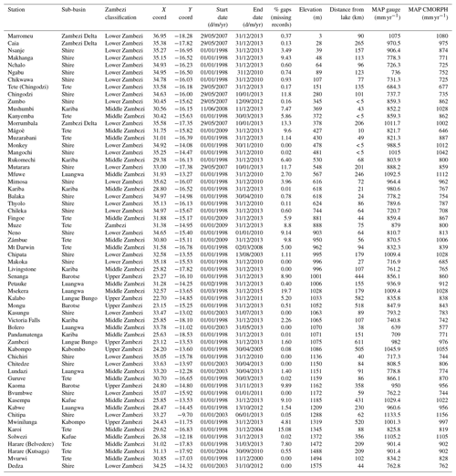
Some stations are affected by data gaps, but the available time series are of sufficiently long duration (see Appendix Table A1) to serve the objectives of this study. Stations are irregularly distributed across the vast basin and are located at an elevation between 3 and 1575 m (Fig. 1). The minimum, maximum, and average distances between the rain gauges are 3.5 km (Zumbo in Mozambique, Kanyemba in Zimbabwe), 1570 km (Mwinilunga in Zambia, Marromeu in Mozambique), and 565 km, respectively. Distances to large-scale open water bodies range between 5 and 615 km. This allows us to evaluate whether elevation and distance to large-scale open water bodies affect CMORPH performance.

3.1.3 Comparison of CMORPH and gauge rainfall

In this study, we compare gauge rainfall at point scale to CMORPH satellite-derived rainfall estimates at pixel scale (point-to-pixel). Comparison is at a daily time interval covering the period 1998–2013, following Cohen Liechti et al. (2012), Dinku et al. (2008), Haile et al. (2014), Hughes (2006), Tsidu (2012), and Worqlul et al. (2014), who report on point-to-pixel comparisons in African basins. We apply point-to-pixel comparison to rule out any aspect of interpolation error as a consequence of the low-density network with unevenly distributed stations. We refer to Heidinger et al. (2012), Li and Heap (2011), Tobin and Bennett (2010), and Yin et al. (2008), who report that interpolation introduces unreliability and uncertainty to pixel-based rainfall estimates. Also, Worqlul et al. (2014) describe that for pixel-to-pixel comparison, there is demand for a well-distributed rain-gauge network that would not hamper accurate interpolation.

3.2 Elevation and distance from large-scale open water bodies

Habib et al. (2012a) and Haile et al. (2009) for the Nile basin reveal that elevation affects the performance of SREs. Findings in the latter two studies signal that performance may possibly also be affected by the presence of Lake Tana. To assess both influences, we classified the Zambezi basin into three elevation zones for which the hierarchical cluster “within-groups linkage” method in the Statistical Product and Service Solutions (SPSS) software was used (Table 1). Based on Euclidian distance to large-scale open water bodies, four arbitrary distance zones are defined to group stations (Table 1). A detailed description of the individual stations, their elevation, and distance to large-scale open water bodies is provided in Table A1. The Advanced Spaceborne Thermal Emission and Reflection Radiometer (ASTER)-based GDEM of 30 m resolution is a product of METI and NASA obtained from https://earthexplorer.usgs.gov/ (last access: 4 July 2019) is used to represent elevation across the Zambezi basin. The Euclidian distance of each rain-gauge location to large-scale open water bodies is defined in a GIS environment through the distance calculation algorithm. Large-scale open water bodies are defined as perennial open water bodies with surface area > 700 km². The threshold is defined based on knowledge of the water bodies in the Zambezi basin study area and the detailed fieldwork the authors have conducted over the years in various other study areas in Africa (such as Lake Tana in Ethiopia and Lake Naivasha in Kenya). The relationship between lake surface area and CMORPH bias on 300 water bodies in the study area shows that at a threshold > 700 km², a signal is induced to warrant the removal from the analysis of all water bodies with surface area < 700 km².

Table 1 Elevation and distance from large-scale open water bodies.

3.3 Bias-correction schemes

Bias-correction schemes evaluated in this study are the spatio-temporal bias (STB), elevation zone bias (EZ), power transform (PT), distribution transformation (DT), and quantile mapping based on an empirical distribution (QME), this by our aim to correct for bias while daily rainfall variability is preserved. The five schemes are chosen based on merits documented in the literature (Bhatti et al., 2016; Habib et al., 2014; Teutschbein and Seibert, 2013; Themeßl et al., 2012; Vernimmen et al., 2012). We note that findings on the performance of selected bias-correction schemes in literature do not allow for generalisation, but findings only apply to the respective study domains (Wehbe et al., 2017; Jiang et al., 2016; Liu et al., 2015; Haile et al., 2015).

In the procedure to define a time window for bias correction we follow Habib et al. (2014) and Bhatti et al. (2016), who in the Lake Tana basin (Ethiopia) carried out a sensitivity analysis of moving time windows and of sequential time windows. Window lengths between 3 and 31 d were tested. Findings indicated that a 7 d sequential time window for bias factors is most appropriate, but only when a minimum of 5 rainy days were recorded within the 7 d window with a minimum rainfall accumulation depth of 5 mm d⁻¹; otherwise, no bias is estimated (i.e. a value of 1 applies as a bias-correction factor). Preliminary tests in this study on 5 and 7 d moving and sequential windows on 20 individual stations distributed over the three elevation zones indicate that the 7 d sequential approach is well applicable in the Zambezi basin. As such, the approach was selected.

The bias-correction factors are calculated using only rain days (rainfall ≥1 mm d⁻¹). Otherwise in cases where both the gauge and satellite have zero values (rain gauge (G) =0 and CMORPH (S) =0), correction is not applied and the SRE value remains 0 mm d⁻¹.

Following Bhatti et al. (2016), we spatially interpolate the bias-correction factors of the rain gauges so that SREs at all pixels can be corrected. For interpolation, the universal kriging was applied. Thus, to systematically correct all CMORPH estimates, station-based bias factors for each time window are spatially interpolated to arrive at spatial coverage across the study area and to allow for comparison with other approaches.

3.3.1 Spatio-temporal bias correction (STB)

This linear bias-correction scheme has its origin in the correction of radar-based precipitation estimates (Tesfagiorgis et al., 2011) and downscaled precipitation products from climate models. The CMORPH daily rainfall estimates (S) are multiplied by the bias-correction factor for the respective sequential time window for individual stations resulting in corrected CMORPH estimates (STB) in a temporally and spatially coherent manner (Eq. 1).

$$\begin{array}{}\text{(1)}& \mathrm{STB}=S{\displaystyle \frac{{\sum }_{t=d}^{t=d-l}G\left(i,t\right)}{{\sum }_{t=d}^{t=d-l}S\left(i,t\right)}},\end{array}$$

where G is gauged rainfall (mm d⁻¹), i is gauge number, d is day number, t is Julian day number, and l is the length of a time window for bias correction.

The advantages of this bias-correction scheme are that it is straightforward and easy to implement due to its simplicity and modest data requirements. However, just like any multiplicative shift procedures of bias correction, STB has challenges in correcting systematic errors in rainfall frequency, particularly the wet-day frequencies (Lenderink et al., 2007; Teutschbein and Seibert, 2013).

3.3.2 Elevation zone bias correction (EZ)

The elevation zone bias-correction scheme is proposed in this study and aims at correcting satellite rainfall for elevation influences. This method groups rain-gauge stations into three elevation zones based on station elevation. The grouping in this study is based on the hierarchical clustering technique and expert knowledge about the study area, but is also guided by recent past studies in the basin (e.g. World Bank, 2010b; Beilfuss, 2012). Each zone has the same bias-correction factor but differs across the three zones. In the time domain bias factors vary following the 7 d sequential window approach. The corrected CMORPH estimates (EZ) at a daily time interval are obtained by multiplying the uncorrected CMORPH daily rainfall estimates (S) by the daily bias-correction factor of each elevation zone.

$$\begin{array}{}\text{(2)}& \mathrm{EZ}=S{\displaystyle \frac{{\sum }_{t=d}^{t=d-l}{\sum }_{i=\mathrm{1}}^{i=n}G\left(i,t\right)}{{\sum }_{t=d}^{t=d-l}{\sum }_{i=\mathrm{1}}^{i=n}S\left(i,t\right)}}\end{array}$$

The merit of this bias-correction scheme is that the effects of elevation on rainfall depth are accounted for. SREs often have difficulties in capturing rainfall events due to orographic effects and thus require elevation-based correction.

3.3.3 Power transform (PT)

The non-linear PT bias-correction scheme has its origin in studies of climate change impact (Lafon et al., 2013). Vernimmen et al. (2012) show that the scheme could be applied to correct satellite rainfall estimates for use in hydrological modelling and drought monitoring. The PT method uses an exponential form to adjust the standard deviation of rainfall series. The daily bias-corrected CMORPH rainfall (PT) for a pixel that overlays a station is obtained using the equation

$$\begin{array}{}\text{(3)}& \mathrm{PT}=aG(i,t{)}^b,\end{array}$$

where G is gauged rainfall (mm d⁻¹), a is a prefactor such that the mean of the transformed CMORPH values is equal to the mean of rain-gauge rainfall, b is a factor calculated such that for each rain gauge the coefficient of variation (CV) of CMORPH matches the gauge-based counterparts, i is the gauge number, and t is the day number.

Optimised values for a and b are obtained through the generalised reduced gradient algorithm (Fylstra et al., 1998). Values for a and b vary for the 7 d sequential window since correction is at a daily time base. In the case of utilising the PT method in a certain area (or for a certain period), the bias-correction factor is spatially interpolated to result in comparable estimates with other bias-correction schemes. The advantage of the bias scheme is that it adjusts extreme precipitation values in CMORPH estimates (Vernimmen et al., 2012). PT has reported limitations in correcting wet-day frequencies and intensities (Leander et al., 2008; Teutschbein and Seibert, 2013).

3.3.4 Distribution transformation (DT)

DT is an additive bias-correction approach which has its origin in statistical downscaling of climate model data (Bouwer et al., 2004). The method transforms a statistical distribution function of daily CMORPH rainfall estimates to match the distribution by gauged rainfall. The procedure to match the CMORPH distribution function to gauge rainfall-based counterparts is described in Eqs. (4)–(8). The principle to matching is that the difference in the mean value and differences in the variance are corrected for in the 7 d sequential window. First, the bias-correction factor for the mean is determined by Eq. (4):

$$\begin{array}{}\text{(4)}& {\mathrm{DT}}_u={\displaystyle \frac{G_u}{S_u}}.\end{array}$$

G_u and S_u are mean values of 7 d gauge and CMORPH rainfall estimates.

Secondly, the correction factor for the variance (DTτ) is determined by the quotient of the 7 d standard deviations, Gτ and Sτ, for gauge and CMORPH, respectively.

$$\begin{array}{}\text{(5)}& \mathrm{DT}\mathit{\tau }={\displaystyle \frac{G\mathit{\tau }}{S\mathit{\tau }}}\end{array}$$

Once the correction factors which vary within a 7 d time sequential window are established, they are then applied to correct all daily CMORPH estimates (S) through Eq. (6) to obtain a corrected CMORPH rainfall estimate (DT). The parameters DT and u are developed within a 7 d sequential window, but correction is at daily time intervals.

$$\begin{array}{}\text{(6)}& \mathrm{DT}=\left(S\right(it)-Su)\mathrm{DT}\mathit{\tau }+\mathrm{DT}u\cdot S\mathit{\tau }\end{array}$$

Uncorrected CMORPH daily values are returned if Eq. (6) results in negative values. The merit of this bias-correction scheme is that it corrects wet-day frequencies and intensities. The disadvantage of this bias-correction scheme is that adding the gauge-based mean deviation to the satellite data destroys the physical consistency of the data. In addition, the method might result in the generation of too few rain days in the wet season, and sometimes the mean of daily intensities might be unrealistically corrected (Johnson and Sharma, 2011; Teutschbein and Seibert, 2013).

3.3.5 Quantile mapping based on an empirical distribution (QME)

This is a quantile-based empirical–statistical error correction method with its origin in empirical transformation and bias correction of regional climate model-simulated precipitation (Themeßl et al., 2012). The method corrects CMORPH precipitation based on empirical cumulative distribution functions (ecdfs) which are established for each 7 d time window and for each station. The bias-corrected rainfall (QME) using quantile mapping is expressed in terms of the empirical cumulative distribution function (ecdf) and its inverse (ecdf⁻¹). Parameters apply to a 7 d sequential window, but correction is then at daily time interval with bias spatially averaged for the entire domain to allow for comparison with other approaches:

$$\begin{array}{}\text{(7)}& \mathrm{QME}={\mathrm{ecdf}}_{\mathrm{obs}}^{-\mathrm{1}}\left({\mathrm{ecdf}}_{\mathrm{raw}}\right(S\left(it\right)\left)\right),\end{array}$$

where ecdf_obs is the empirical cumulative distribution function for the gauge-based observation and ecdf_raw is the empirical cumulative distribution function for the uncorrected CMORPH.

The advantage of this bias scheme is that it corrects quantiles and preserves the extreme precipitation values (Themeßl et al., 2012). However, it also has its limitation due to the assumption that both the observed rainfall and satellite rainfall follow the same proposed distribution, which may introduce potential new biases.

3.4 Rainfall rates and seasons

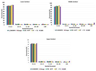
To assess the performance of SREs for different classes of daily rainfall rates, five classes are defined which indicate very light (< 2.5 mm d⁻¹), light (2.5–5.0 mm d⁻¹), moderate (5.0–10.0 mm d⁻¹), heavy (10.0–20.0 mm d⁻¹), and very heavy (> 20.0 mm d⁻¹) rainfall.

Furthermore, gauged rainfall was divided into wet and dry seasonal periods to assess the influence of seasonality on performance of bias-correction schemes. The wet season in the Zambezi basin spans from October to March, whereas the dry season spans from April to September.

3.5 Evaluation of CMORPH estimates

Corrected and uncorrected CMORPH satellite rainfall estimates are evaluated with reference to rain-gauge rainfall using statistics that measure systematic differences (i.e. percentage bias and mean absolute error (MAE)), measures of association (e.g. correlation coefficient and Nash–Sutcliffe efficiency – NSE), and random differences (e.g. standard deviation of differences and coefficient of variation) (Haile et al., 2013). Bias is a measure of how the satellite rainfall estimate deviates from the rain-gauge rainfall, and the result is normalised by the summation of the gauge values (Rientjes et al., 2013). A positive value indicates overestimation, whereas a negative value indicates underestimation. The correlation coefficient (ranging between +1 and −1) represents the linear dependence of gauge and CMORPH data. MAE is the arithmetic average of the absolute values of the differences between the daily gauge and CMORPH satellite rainfall estimates. The MAE is zero if the rainfall estimates are perfect and increases as discrepancies between the gauge and satellite become larger. NSE indicates how well the satellite rainfall matches the rain-gauge observation, and it ranges between −∞ and 1, with NSE =1 meaning a perfect fit (Nash and Sutcliffe, 1970).

Equations (8)–(11) apply.

$$\begin{array}{}\text{(8)}& {\displaystyle }\mathrm{bias}\left(\mathit{\%}\right)={\displaystyle \frac{\sum (S-G)}{\sum G}}\cdot \mathrm{100},\text{(9)}& {\displaystyle }R={\displaystyle \frac{\sum (G-\stackrel{\mathrm{‾}}{G})(S-\stackrel{\mathrm{‾}}{S})}{\sqrt{\sum (G-\stackrel{\mathrm{‾}}{G}{)}^{\mathrm{2}}}\sqrt{\sum (S-\stackrel{\mathrm{‾}}{S}{)}^{\mathrm{2}}}}},\text{(10)}& {\displaystyle }\mathrm{MAE}={\displaystyle \frac{\mathrm{1}}{n}}\sum \mathrm{|}S-G\mathrm{|},\text{(11)}& {\displaystyle }\mathrm{NSE}={\displaystyle \frac{\sum (G-S{)}^{\mathrm{2}}}{\sum (G-\stackrel{\mathrm{‾}}{G}{)}^{\mathrm{2}}}},\end{array}$$

where S are satellite rainfall estimates (mm d⁻¹), $\stackrel{\mathrm{‾}}{S}$ is the mean of the satellite rainfall estimates (mm d⁻¹), G is rainfall by a rain gauge (mm d⁻¹), $\stackrel{\mathrm{‾}}{G}$ are mean values of rainfall recorded by a rain gauge (mm d⁻¹), and n is the number of observations.

3.6 Test for differences of mean

To detect significant differences between gauge and satellite rainfall (corrected and uncorrected) and differences amongst the five bias-correction methods described in Sect. 3.3, we apply a paired t test and analysis of variance (ANOVA) tests.

3.6.1 Paired t tests

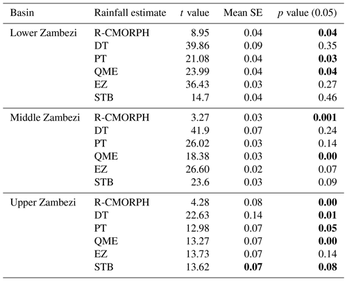
A paired t test was used to test whether there is a significant difference between rain-gauge, uncorrected, and bias-corrected CMORPH satellite rainfall for the 52 rain gauges. Results are summarised for the Upper, Lower, and Middle Zambezi. The paired t test compares the mean difference of the values to zero. It depends on the mean difference, the variability of the differences, and the number of data. The null hypothesis (H₀) is that there is no difference in mean gauge and satellite daily rainfall (uncorrected and bias corrected). If the p value is less than or equal to 0.05 (5 %), the result is deemed statistically significant, i.e. there is a significant relationship between the gauge and satellite rainfall (Wilks, 2006).

3.6.2 Analysis of variance (ANOVA) test

The ANOVA test aims to test whether there is a significant difference amongst the five bias-correction techniques. The null hypothesis (H₀) is that there are no differences amongst the five bias-correction schemes. We further determined which schemes differ significantly using three post hoc tests, namely Tukey HSD, Scheffe, and Bonferroni (Brown, 2005; Kucuk et al., 2018). Results are summarised for the Upper, Lower, and Middle Zambezi.

3.7 Taylor diagram

We apply a Taylor diagram to evaluate differences in data sets generated by respective bias-correction schemes by providing a summary of how well bias-correction results match gauge rainfall in terms of pattern, variability, and magnitude of the variability. Visual comparison of SRE performance is done by analysing how well patterns match each other in terms of Pearson's product-moment correlation coefficient (R), root mean square difference (E), and the ratio of variances on a 2-D plot (Lo Conti et al., 2014; Taylor, 2001). The reason that each point in the 2-D space of the Taylor diagram can represent the above three different statistics simultaneously is that the centered pattern of root mean square difference (Eⁱ) and the ratio of variances are related by the following:

$$\begin{array}{}\text{(12)}& E^i=\sqrt{{\mathit{\sigma }}_f^{\mathrm{2}}+{\mathit{\sigma }}_r^{\mathrm{2}}-\mathrm{2}{\mathit{\sigma }}_f{\mathit{\sigma }}_{r}R},\end{array}$$

where σ_f and σ_r are the standard deviation of CMORPH and rain-gauge rainfall, respectively.

Development and applications of Taylor diagrams have roots in climate change studies (Smiatek et al., 2016; Taylor, 2001) but also have frequent applications in environmental model evaluation studies (Cuvelier et al., 2007; Dennis et al., 2010; Srivastava et al., 2015). Bhatti et al. (2016) propose the use of Taylor diagrams for assessing effectiveness of SRE bias-correction schemes. The most effective bias-correction schemes will have data that lie near a point marked “reference” on the x axis, a relatively high correlation coefficient, and a low root mean square difference. Bias-correction schemes matching gauge-based standard deviation have patterns that have the right amplitude.

3.8 Quantile–quantile (q–q) plots

A q–q plot is used to check whether two data sets (in this case gauge vs. CMORPH rainfall) can fit the same distribution (Wilks, 2006). A q–q plot is a plot of the quantiles of the first data set against the quantiles of the second data set. A 45^∘ reference line is also plotted. If the satellite rainfall (corrected and uncorrected) has the same distribution as the rain gauge, the points should fall approximately along this reference line. The greater the departure from this reference line, the greater the evidence for the conclusion that the bias-correction scheme is less effective (NIST/SEMATECH, 2001).

The main advantage of the q–q plot is that many distributional aspects can be simultaneously tested. For example, changes in symmetry, and the presence of outliers, can all be detected from this plot.

3.9 Cross-validation of bias correction

3.9.1 Spatial cross-validation

The spatial cross-validation procedure (hold-out sample) applied in this study involves the withdrawal of 8 in situ stations from the sample of 60 when generating bias-corrected SREs for all pixels across the study area. Corrected SREs are then compared to the rain-gauge rainfall of the withdrawn stations to evaluate closeness of match. From the sample of eight we selected two stations in the < 250 m elevation zone, three stations in the 250–950 m zone, and three stations in the > 950 m elevation zone. Stations selected have elevation close to the average elevation zone value and are centred in an elevation zone. This left us with 52 stations for applying the bias-correction methods and spatial interpolation. As performance indicators to evaluate results of cross-validation, we use the percentage bias, MAE, correlation coefficient, and the estimated ratio which is obtained by dividing CMORPH rainfall totals and gauge-based rainfall totals for the 1999–2013 period.

3.9.2 Temporal cross-validation

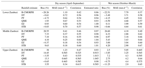
For evaluation of SREs in the time domain we followed Gutjahr and Heinemann (2013) in omitting rainfall (from both gauge and satellite) for the 1998–1999 hydrological year to remain with 14 years for bias correction of SREs. Bias-corrected estimates for the 14 years are then evaluated against estimates for the 1998–1999 period that served as a reference. For evaluation we use the percentage bias, MAE, correlation coefficient, and the estimated ratio, which all are averaged for the Upper, Middle, and Lower Zambezi but also for the wet and dry seasons.

4 Results and discussion

4.1 Performance of uncorrected CMORPH rainfall

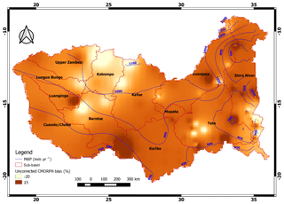
The spatially interpolated values of bias (%) across the Zambezi basin are shown in Fig. 2. Areas in the central and western parts of the basin have bias relatively close to zero, suggesting good performance of the uncorrected CMORPH product. However, relatively large negative bias values (−20 %) are shown in the Upper Zambezi's high-elevation areas such as Kabompo and the northern Barotse basin, in the south-eastern part of the basin such as the Shire River basin, and in the Lower Zambezi's downstream areas where the Zambezi River enters the Indian Ocean. CMORPH overestimates rainfall locally in the Kariba, Luanginga, and Luangwa basins by positive bias values. As such CMORPH estimates do not consistently provide results that match rain-gauge observations. Since CMORPH estimates have pronounced error (−10 > bias (%) > 10), bias needs to be removed before the product can be applied for hydrological analysis and in water resource applications. Figure 2 also shows contours for rain-gauge mean annual precipitation (MAP) in the Zambezi basin, with higher values in the northern parts of the basin (Kabompo and Luangwa) compared to localised estimates of MAP such as in the Shire River and Kariba sub-basins.

Figure 2 The spatial variation of bias (%) for gauge vs. uncorrected CMORPH daily rainfall (1998–2013) for the Zambezi basin. The gauge-based isohyets for mean annual precipitation (MAP) are shown in blue.

4.2 Effects of elevation and distance from large-scale open water bodies on CMORPH bias

Figure 3 shows Taylor diagrams with a comparison of basin lumped estimates of daily uncorrected time series (1999–2013) of CMORPH and gauge-based rainfall for the three elevation zones (Fig. 3a) and four distance zones from large-scale open water bodies (Fig. 3b). Here CMORPH performance is indicated by means of the root mean square difference (E), correlation coefficient (R), and standard deviation. Figure 3a and b show that standard deviations in the elevation zones and the distance zones (except for the < 10 km distance zone) are lower than the reference/rain-gauge standard deviation which is indicated by the black arc (value of 8.45 mm d⁻¹). The stations in the high-elevation zone (> 950 m) and long-distance zone (> 100 km) reveal lower variability than stations in lower-elevation and shorter-distance zones. With respect to the reference line, CMORPH estimates that are lumped for respective elevation zones and distance to a large water body do not match the standard deviations of rain-gauge-based counterparts. Figure 3a and b also show that CMORPH standard deviations that are close to gauge-based rainfall apply to lower-elevation and shorter-distance zones. Based on the Taylor diagrams, the statistics (R and E) for uncorrected CMORPH show increasing performance for increasing elevation and increasing distance from large-scale water bodies. Specifically, stations in the lower-elevation zones (< 250 m) have lower R and higher E than the higher-elevation zones (> 950 m). For shorter-distance zones lower R and higher E are shown than for longer-distance zones (> 100 km). These findings suggest that in general effects of distance to a large-scale water body are minimal except for distances < 10 km.

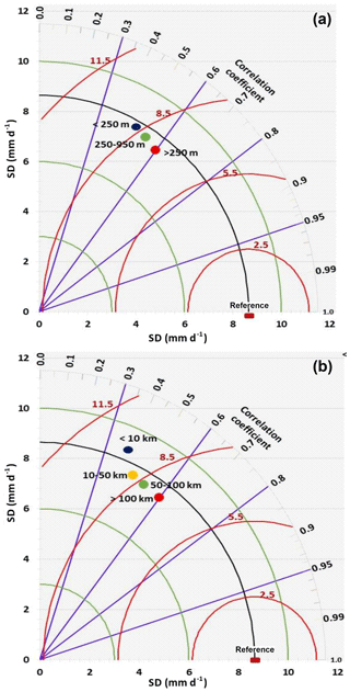
Figure 3 (a) Elevation zones. (b) Distance zones. Time series of rain-gauge (reference) vs. CMORPH estimations, period 1999–2013, for elevation zones (a) and distance zones (b) in the Zambezi basin. The correlation coefficients for the radial line denote the relationship between CMORPH and gauge-based observations. Standard deviations on both the x and y axes show the amount of variance between the two time series. The standard deviation of the CMORPH pattern is proportional to the radial distance from the origin. The angle between symbol and abscissa measures the correlation between CMORPH and rain-gauge observations. The root mean square difference (red contours) between the CMORPH and rain-gauge patterns is proportional to the distance to the point on the x axis identified as “reference”. For details, see Taylor (2001).

4.3 Evaluation of bias correction

4.3.1 Standard statistics

Figure 4 shows frequency-based statistics (mean and maximum) on the accuracy of CMORPH rainfall estimates for each bias-correction method. The ratios of cumulated estimates (1999–2013) from rain-gauge and CMORPH estimates for the Lower, Middle, and Upper Zambezi sub-basins are shown. Results show that the bias of CMORPH moderately reduced for each of the five bias-correction schemes. However, the effectiveness of the schemes varies spatially, with the best performance in the Lower and Upper Zambezi sub-basin and relatively poor performance in the Middle Zambezi sub-basin (see Fig. 4).

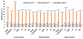
Figure 4 Frequency-based statistics (mean, max, and estimated ratio of gauged sum vs. CMORPH sum for 1999–2013) of corrected CMORPH for the Lower, Middle, and Upper Zambezi basin.

Judging by the three performance indicators (mean, max, and estimated ratio), results indicate that the STB bias-correction scheme is consistently effective in removing CMORPH rainfall bias in the Zambezi basin. STB and PT effectively adjust for the mean of CMORPH rainfall estimates. Statistics in Fig. 5 confirm these findings especially for the Upper Zambezi sub-basin, where the mean of corrected estimates improved by > 60 % from the mean of uncorrected estimates. In addition, PT in the Lower Zambezi, QME in both the Middle and Upper Zambezi, and STB in the Upper Zambezi were also effective (improvement by 16 %) in correcting for the highest values in the rainfall estimates. STB performs better than other bias schemes in reproducing rainfall for the Lower and Upper Zambezi sub-basin, where the ratio of gauge total to corrected CMORPH total is close to 1.0.

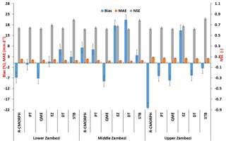
Figure 5 Percentage bias, mean absolute error (left axis), and Nash–Sutcliffe efficiency (NSE) (right axis) of corrected and uncorrected CMORPH (R-CMORPH) daily rainfall averaged for the Lower Zambezi, Middle Zambezi, and Upper Zambezi for the 1999–2013 period.

Figure 5 shows the MAE and percentage bias (% bias) on the left axis and NSE on the right axis as measures to evaluate performance of bias-correction schemes in the Zambezi basin. The effectiveness of the bias correction by all schemes varies over the different parts of the basin, but is higher in the Lower and Upper Zambezi than in the Middle Zambezi. The STB, PT, and EZ show improved performance by exhibiting smaller MAEs compared to the uncorrected CMORPH (R-CMORPH). A greater improvement is shown for the Middle Zambezi, where the uncorrected MAE of 1.89 mm d⁻¹ is reduced to 0.86 mm d⁻¹ after bias correction by the elevation zone bias-correction scheme (EZ). The signal on improved performance for the Lower and Middle Zambezi as compared to the Upper Zambezi is also evident for the majority of the bias-correction techniques. However, relatively large error remains in the MAE.

NSE for STB is larger than 0.8 for all three Zambezi sub-basins. This is followed by EZ with NSE larger than 0.7 for the three sub-basins. The lowest NSE is for QME, which is close to 0.65 for all three sub-basins. The best results for reducing bias (% bias) are obtained by EZ in the Lower Zambezi (% bias of 0.7 % ∼ absolute bias of 0.10 mm d⁻¹) and Upper Zambezi (0.22 % ∼0.23 mm d⁻¹), PT in the Lower and Middle Zambezi (−0.84 % ∼0.18 mm d⁻¹), and STB in all the basins (< 3.70 % ∼0.24 mm d⁻¹). Gao and Liu (2013) over the Tibetan Plateau assert that EZ is valuable in correcting systematic biases to provide a more accurate precipitation input for rainfall–runoff modelling. Significant underestimation for the uncorrected (−21.16 % ∼0.44 mm d⁻¹) and bias-corrected CMORPH is shown for the Upper Zambezi sub-basin.

4.3.2 Significance testing

Table 2 shows results of statistical tests to assess whether there is a significant difference (p < 0.05) between rain-gauge vs. uncorrected and bias-corrected CMORPH satellite rainfall for each of the 52 rain-gauge stations. Results are summarised for the Upper, Middle, and Lower Zambezi and in the Zambezi basin. The null hypothesis is rejected for PT (Lower Zambezi), DT (Upper Zambezi), and QME (all three sub-basins) since p < 0.05. This means that statistically the above-mentioned bias-correction schemes results deviate from the gauge. The null hypothesis is accepted for STB and EZ (all three sub-basins), DT (Lower and Upper Zambezi), and PT (Middle and Upper Zambezi), since p > 0.05, showing the effectiveness of these bias-correction schemes. Compared to uncorrected satellite rainfall (R-MORPH), results also reveal that the bias-corrected satellite rainfall is closer to the gauge-based rainfall.

Table 2 Paired t tests for the Upper, Middle, and Lower Zambezi. The mean difference is significant at the 0.05 level. Bold shows significant values.

4.3.3 Analysis of variance (ANOVA test)

The ANOVA test is similar to a t test, except that the test was used to compare mean values from three or more data samples. Results of ANOVA show that there is a significant (p < 0.05) difference in the mean values of the five bias-correction results across the three sub-basins. This warranted the running of a post hoc test to determine which schemes differ significantly. The contingency matrix in Table 3 shows results of the post hoc test results summarised for the Tukey HSD, Scheffe, and Bonferroni methods but also for the Upper, Lower, and Middle Zambezi. Table 3 also shows that STB, PT, and EZ are significantly different from distribution transformation (DT) for the three sub-basins. STB, the best performing bias-correction scheme identified, is also significantly different from QME and EZ. QME, which has performed poorly, is significantly different from EZ. Results are important for further application of the bias-correction schemes for studies such as flood, drought, and water resource modelling.

Table 3 ANOVA post hoc tests for the results of the five bias-correction schemes (p < 0.05). The checklist table gives an indication (symbol) where two bias-correction schemes' results are significantly different from each other. Where there is no symbol, it means that the schemes' results are not significantly different. The different symbols represent the Upper, Middle, and Lower Zambezi basins.

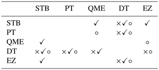
Key: × – Upper Zambezi, ✓ – Lower Zambezi, ∘ – Middle Zambezi

4.3.4 Taylor diagrams

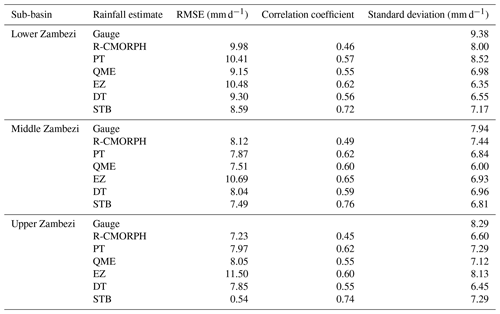
Figure 6 shows the Taylor diagram for time series of rain-gauge (reference) observations vs. CMORPH bias-correction schemes averaged for the Lower Zambezi (UZ), Middle Zambezi (MZ), and Upper Zambezi (UZ). Absolute values used to develop the Taylor diagram are shown in Table A2. The position of each bias-correction scheme and uncorrected satellite rainfall (R-MORPH) in Fig. 6 shows how closely the rainfall by uncorrected CMORPH (R-MORPH) matches rain-gauge observations as well as the effectiveness of each of the bias-correction schemes. Overall, all bias-correction schemes show intermediate performance in terms of bias removal. Only the PT and STB for the Lower Zambezi sub-basin lie on the line of standard deviation (brown dashed arc) and means the standard deviations of the data for the two bias-correction schemes match the gauge observations. This also indicates that rainfall variations after PT and STB bias correction for the Lower Zambezi resemble gauge-based standard deviation. Note however that STB performs better than EZ, as shown by the superior correlation coefficient. Compared against the reference line of the mean standard deviation (8.5 mm d⁻¹), the rainfall standard deviation for most bias-correction schemes is below this line and as such exhibits low variability across the Zambezi basin.

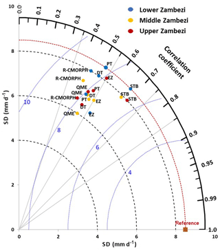
Figure 6 Taylor's diagram on rain-gauge (reference) observations and CMORPH bias-corrected estimates (all five schemes) as averaged for the Lower Zambezi (LZ), Middle Zambezi (MZ), and Upper Zambezi (UZ) for the period 1999–2013. The distance of the symbol from point (1, 0) is also a relative measure of the bias-correction scheme performance. The position of each symbol appearing on the plot quantifies how closely precipitation estimates by a respective bias-correction scheme match counterparts by rain gauges. The dashed blue lines indicate the root mean square difference (mm d⁻¹).

Figure 6 also shows that most of the bias-correction schemes have a standard deviation range of 6.0 to 8.0 mm d⁻¹. There is a consistent pattern between the bias-correction schemes that have low R and high RMSE difference, indicating that these schemes are not effective in bias removal. Overall, the best-performing bias-correction schemes (STB and EZ) have R > 0.6, standard deviation relatively close to the reference point, and RMSE < 7 mm d⁻¹. The uncorrected CMORPH (R-MORPH) lies far away from the marked reference (gauge) point on the x axis, suggesting an intermediate overall effectiveness of the bias-correction schemes such as STB, EZ, DT, and PT in removing error as they are relatively closer to the marked reference point.

The least-performing bias-correction scheme is QME, with relatively large RSMD (> 8 mm d⁻¹) and with low R (< 0.49) and standard deviation (< 6.5 mm d⁻¹). Inherent to the methodology of most of the bias-correction schemes (e.g. QME) is that the spatial pattern of the SRE does not change, and therefore R for a specific station for daily precipitation does not necessarily improve. The bias-correction results by the Taylor diagram in Fig. 6 corroborate findings shown in Figs. 4 and 5 for mean, max, ratio of rainfall totals, and bias as performance indicators.

4.3.5 q–q plots

Figure 7 shows q–q plots for the Upper, Middle, and Lower Zambezi for gauge rainfall against uncorrected and bias-corrected CMORPH rainfall. Results show that STB's q–q plots for bias-corrected CMORPH across the three basins have the majority of points that fall approximately along the 45^∘ reference line. This means that the STB bias-corrected satellite rainfall has closer distribution to the rain gauge as compared to the uncorrected CMORPH counterparts, suggesting the effectiveness of the bias-correction scheme. Other bias-correction schemes such as QME, EZ, and PT have data points showing a greater departure from the 45^∘ reference line, so performance is less effective.

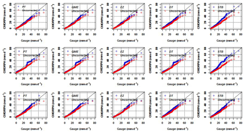
Figure 7 q–q plot for gauge vs. satellite rainfall (uncorrected and bias corrected) for the Upper (top panels), Middle (middle panes), and Lower (bottom panels) Zambezi.

In some instances, in the Upper, Middle, and Lower Zambezi, bias-corrected values are significantly higher than the corresponding gauge values, whereas in some instances there is serious underestimation. All the q–q plots also show that for all the bias-correction schemes, the differences between gauge and satellite rainfall are smallest for low rainfall rates (< 2.5 mm d⁻¹) and increasing for very heavy rainfall (> 20.0 mm d⁻¹). In more detail, all the bias-correction schemes show a larger difference for the transition area from low to heavy rainfall. QME and PT are not in good agreement with the rest of the bias-correction schemes for higher rainfall estimates (40 and 60 mm d⁻¹).

4.3.6 CMORPH rainy days

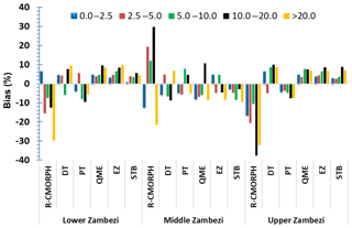
Occurrence (%) of rainfall rates in the Zambezi basin for each bias-correction scheme is shown in Fig. 8. The highest percentage (80 %–90 %) is shown for very light rainfall (0.0–2.5 mm d⁻¹). A smaller percentage is shown for 2.5–5.0 mm d⁻¹, which is the light rainfall class. The smallest percentage (< 5 %) is shown for very heavy rainfall (> 20 mm d⁻¹). The CMORPH rainfall corrected with STB, PT, and DT matches the gauge-based rainfall (%) in the Lower, Middle, and Upper Zambezi, suggesting good performance. All five bias-correction schemes in the Zambezi basin generally tend to overestimate very light rainfall (< 2.5 mm d⁻¹). There is a small difference for moderate rainy day classification of 10.0–20.0 mm d⁻¹. For QME in the Middle and Upper Zambezi, there is overestimation by > 80 %. There is underestimation of rainfall greater than 20 mm d⁻¹.

Figure 8 Percentage occurrence for rainfall rate classes.

Figure 9 gives the bias-correction performance for the different rainy-day classes. Results of bias removal vary for the Lower, Middle, and Upper Zambezi. Comparatively, the STB and EZ show effectiveness in bias removal with average bias corrections of 0.97 % and 3.6 % in the whole basin, respectively. Results show more effectiveness in reducing the percentage bias for light (2.5–5.0 mm d⁻¹) and moderate (5.0–10.0 mm d⁻¹) rainfall compared to the heavy (10.0–20.0 mm d⁻¹) and very heavy (> 20.0 mm d⁻¹) rainfall across the whole basin.

Figure 9 Bias correction (%) for the respective rainfall rate (mm d⁻¹) classes.

4.4 Spatial cross-validation

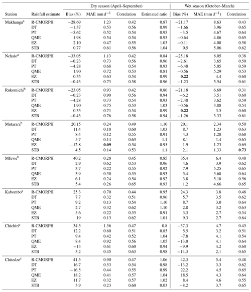
Table 4 shows the cross-validation results on bias correction for eight rain-gauge stations in the wet and dry seasons. It is evident that CMORPH has a considerable bias, although this bias is not always consistent for all eight validation stations. Overall, Mutarara station has the highest positive bias (overestimation), whereas Makhanga has the highest negative bias (underestimation) for uncorrected CMORPH. Bias is effectively being removed by the STB followed by the EZ bias-correction schemes. Bias is more effectively removed for the wet season than for the dry season. For the dry season, the STB shows good performance for Mkhanga and Nchalo stations, whereas good performance is shown for Kabompo and Chichiri stations. However, the MAE is higher for the wet season than for the dry season. The correlation coefficient for bias-corrected satellite rainfall is higher for the wet season than for the dry season.

Table 4 Cross-validation results for the bias-correction procedure with eight gauging stations for the dry and wet seasons. Stations lie in an average elevation zone and are sort of centred in an elevation zone. R-CMORPH is the uncorrected R-CMOPRPH estimate. DT, PT, QME, EZ, and STB are the bias-corrected rainfall estimate. Bold values indicate best performance. ^a Zone 1: elevation of < 250 m; ^b zone 2: elevation range of 250–950 m; and ^c zone 3: elevation > 950 m.

4.5 Temporal cross-validation

The same performance indicators in spatial cross-validation are calculated for the temporal cross-validation. Results are presented in Table 5. The MAE is higher for the wet season than for the dry season. The difference in effectiveness in the error removal between the dry and wet seasons is much larger. STB outperforms both bias-correction methods but does also have problems correcting the estimated ratios. After the correction, the correlation coefficient is much improved. The fact that MAE remains relatively large indicates that errors remain locally large. These values are almost in the same range as performance indicators obtained from the main performance assessment period (1999–2013). The estimated ratio shows improvement for the Middle Zambezi compared to the Lower and Upper Zambezi.

Table 5 Temporal cross-validation results for the period 1998–1999 for the wet and dry seasons.

5 Discussion

We present methods to assess the performance of bias-correction schemes for CMORPH rainfall estimates in the Zambezi River basin. For correction we applied sequential windows of 7 d that count 5 rain days with a rainfall threshold of 5 mm d⁻¹. First, we aimed to evaluate whether performance of CMORPH rainfall is affected by elevation and distance from large-scale open water bodies. Results in Taylor diagrams show that effects of distances > 10 km are minimal in this study. For distance < 10 km, results in the same Taylor diagrams show some effect with increased CMORPH estimation errors, although this is not clearly identifiable by the limited number of gauging stations at distance < 10 km. The low number of gauge stations constrains clear identification of bias as affected by the short distance. The low number of stations also constrains detailed analysis of dependencies of observation time series. To assess bias effects at distances < 10 km we advocate installation of a well-designed network of rain gauges with stations located at preselected locations that would allow sound geostatistical analysis of small-scale rainfall variability and spatial correlation analysis. We refer to Ciach and Krajewski (2006), who present such analysis for a dense experimental network of 53 stations. The inter-station distance of the rain gauges in this study is too large to capture the effect of distance to large-scale open water bodies on CMORPH rainfall error. For instance, such distance exceeds 350 km for most of the Upper Zambezi basin. Findings in this study show that effects of distance would be captured at distances 10–25 km or shorter. Haile et al. (2009) indicate bias effects at short distances (< 10 km) for the Lake Tana, Ethiopia.

The rainfall-elevation bias correction also shows minimal signal. Contrary to this finding, Romilly and Gebremichael (2011) showed that the accuracy of CMORPH at a monthly time base is related to elevation for six river basins in Ethiopia. A similar finding was reported by Haile et al. (2009), Katiraie-Boroujerdy et al. (2013), and Wu and Zhai (2012), who found that the performance of CMORPH is affected by elevation. However, Vernimmen et al. (2012) concluded that TRMM Multi-satellite Precipitation Analysis (TMPA) 3B42RT performance was not affected by elevation (R²=0.0001) for the Jakarta, Bogor, Bandung, Java, Kalimantan, and Sumatra regions (Indonesia). The study by Gao and Liu (2013) showed that the bias in CMORPH rainfall over the Tibetan Plateau is affected by elevation. Whilst distances from large-scale open water bodies and elevation have been assessed separately for this study, Habib et al. (2012a) revealed that both aspects interact in the Nile basin to produce unique circulation patterns to affect the performance of SRE.

Secondly, we evaluate the effectiveness of linear/non-linear and time–space-variant/-invariant bias-correction schemes. The bias-correction results by means of performance indicators such as Taylor diagrams, q–q plots, ANOVA, and standard statistics such as mean, max, ratio of rainfall totals, and bias reveal that the STB is the best bias-correction method. This method by its nature considers correction only for spatially distributed patterns in bias, commonly known as space-variant/-invariant, and thus forces the estimates to behave as observations. We did not investigate effects of the applied sequential windows of 7 d for each bias-correction scheme separately, but note that other window lengths possibly could yield more favourable results for bias schemes such as PT, DT, and QME that commonly rely on larger sample sizes. As alluded to by Habib et al. (2014), correction should improve hydrological applications by improved rainfall representation. This applies to the Zambezi basin as well with demands for applications of the product such as for drought analysis, flood prediction, weather forecasting, and rainfall–runoff modelling. The study is unique as we assess the importance of space and time aspects of CMORPH bias for rainfall–runoff modelling in a data-scarce catchment. Findings in this study on cross-validation and temporal validation contribute to efforts that aim towards enhancing applications of satellite rainfall products. The study site is the Zambezi basin, an example of many world regions that can benefit from satellite-based rainfall products for resource assessments and monitoring.

Thirdly, an assessment of the performance of bias-correction schemes in representing different rainfall rates and climate seasonality is presented. Our findings show that bias is most overestimated for the very light rainfall (< 2.5 mm d⁻¹), which is also the range that shows the best bias reduction, which in turn is most effective during the wet season. Results also show that there is underestimation of rainfall larger than 20 mm d⁻¹. The poor performance of correction for the heavy rainfall class is caused by, sometimes, large mismatch of high rain-gauge values vs. low CMORPH values. This leads to unrealistically high CMORPH values which remain poorly corrected by bias schemes. Results are consistent with findings by Gao and Liu (2013) in the Tibetan Plateau, who found consistent underestimation and overestimation of occurrence by CMORPH for rainfall rates > 10 mm d⁻¹. A study by Zulkafli et al. (2014) in French Guiana and North Brazil noted that the low sampling frequency and consequently missed short-duration precipitation events between satellite measurements results in underestimation, particularly for rainfall > 20 mm d⁻¹.

Lastly, spatial and temporal cross-validation reveals the effectiveness of bias-correction schemes. The hold-out sample of eight stations in this work showed the applicability of different bias-correction methods under different geographical domains. There is improved performance of satellite rainfall for the wet season as compared to the dry season based on the correlation coefficient and MAE. The study by Ines and Hansen (2006) for semi-arid eastern Kenya showed that multiplicative bias-correction schemes such as STB were effective in correcting the total of the daily rainfall grouped into seasons. Our results show that effectiveness in bias removal in the wet season is higher than in the dry season. This is contrary to Vernimmen et al. (2012), who showed that for the dry season, bias for PT decreased in the Jakarta, Bogor, Bandung, East Java, and Lampung regions after bias correction of monthly TMPA 3B42RT precipitation estimates over the period 2003–2008. Habib (2014) evaluated the sensitivity of STB for the dry and wet seasons and concluded that the bias-correction factor for CMOPRH shows lower sensitivity for the wet season as compared to the dry season. Our findings also reveal that bias factors for all the schemes are more variable in the dry season than in the wet season and lead to poor performance of the bias-correction schemes in the dry season.

6 Conclusions

In this study four conclusions are drawn.

1. Analysis of gauge and CMORPH rainfall estimates shows that CMORPH performance increases for higher elevation (> 950 m) in the Zambezi basin and that CMORPH has the largest mismatch at low elevation. Such analysis was established for rain gauges within elevation zone classes of < 250, 250–950, and > 950 m. The match between gauge and CMORPH estimates improved at increasing distance to large-scale open water bodies. This was established for rain gauges located within specified distances of 10–50, 50–100, and > 100 km to a large-scale open water body. For distances < 10 km errors by CMORPH increased, but the small sample size of stations and the weak signal require further study. To assess how bias is affected at short distances to a large-scale water body, a specifically designed and dense gauging network is advocated (see Ciach and Krajewski, 2006) that allows evaluation of small-scale rainfall variability. A detailed analysis of small spatial variability and spatial correlation analysis of rain-gauged observations presumably is a prerequisite before satellite rainfall effects at short distances to a large-scale water body can be assessed.

2. For each of the five bias-correction methods applied, accuracy of the CMORPH satellite rainfall estimates improved. Assessment through standard statistics, Taylor diagrams, t tests, ANOVA, and q–q plots shows that STB that accounts for space and time variation of bias is found to be more effective in reducing satellite rainfall bias in the Zambezi basin than the rest of the bias-correction schemes. This indicates that the temporal aspect of CMORPH bias is more important than the spatial aspect in the Zambezi basin. Quantile–quantile (q–q) plots for all the bias-correction schemes in general show that bias-corrected rainfall is in good agreement with gauge-based rainfall for low rainfall rates but that high rainfall rates are largely overestimated.

3. Differences in the mechanisms that drive precipitation throughout the year could result in different biases for each of the seasons, which motivated us to calculate the bias-correction factors for dry and wet seasons separately. As such, CMORPH rainfall time series were divided to assess the influence of seasonality on the performance of bias-correction schemes. Overall, the bias-correction schemes reveal that bias removal is more effective in the wet season than in the dry season.

4. We assessed whether bias correction varies for different rainfall rates of daily rainfall in the Zambezi basin. There is overestimation of very light rainfall (< 2.5 mm d⁻¹) and underestimation of very heavy rainfall (> 20 mm d⁻¹) after application of the bias-correction schemes. Bias was more effectively reduced for the very light (< 2.5 mm d⁻¹) to moderate (5.0–10.0 mm d⁻¹) rainfall compared to the heavy (10.0–20.0 mm d⁻¹) and very heavy (> 20 mm d⁻¹) rainfall. Overall, the STB and EZ more consistently removed bias in all the rainy days' classification compared to the three other bias-correction schemes. Effects of length of sequential window sizes for selected bias-correction schemes are not investigated, but different lengths possibly could yield more favourable results for PT, QME, and DT bias-correction schemes.

Analysis serves to improve the reliability of SRE applications in hydrological analysis and water resource applications in the Zambezi basin such as in drought analysis, flood prediction, weather forecasting, and rainfall–runoff modelling. In follow-up studies, we aim at hydrologic evaluation of bias-corrected CMORPH rainfall estimates at the headwater catchment of the Zambezi River.

Appendix A

Table A1 Rain-gauge stations in the Zambezi sub-basins showing x and y locations, sub-basin they belong to, year of data availability, % of missing gaps, station elevation, and distance from large-scale water bodies.

Table A2 Bias-correction scheme-based Taylor diagram performance indicators (correlation coefficients, standard deviations, and RMSE) of rain-gauge (reference) vs. CMORPH estimations (corrected and uncorrected), period 1998–2013, for the Lower, Middle, and Upper Zambezi basin.