Mapping soil hydraulic properties using random-forest-based pedotransfer functions and geostatistics

Spatial 3-D information on soil hydraulic properties for areas larger than plot scale is usually derived using indirect methods such as pedotransfer functions (PTFs) due to the lack of measured information on them. PTFs describe the relationship between the desired soil hydraulic parameter and easily available soil properties based on a soil hydraulic reference dataset. Soil hydraulic properties of a catchment or region can be calculated by applying PTFs on available soil maps. Our aim was to analyse the performance of (i) indirect (using PTFs) and (ii) direct (geostatistical) mapping methods to derive 3-D soil hydraulic properties. The study was performed on the Balaton catchment area in Hungary, where density of measured soil hydraulic data fulfils the requirements of geostatistical methods. Maps of saturated water content (0 cm matric potential), field capacity (−330 cm matric potential) and wilting point (−15 000 cm matric potential) for 0–30, 30–60 and 60–90 cm soil depth were prepared. PTFs were derived using the random forest method on the whole Hungarian soil hydraulic dataset, which includes soil chemical, physical, taxonomical and hydraulic properties of some 12 000 samples complemented with information on topography, climate, parent material, vegetation and land use. As a direct and thus geostatistical method, random forest combined with kriging (RFK) was applied to 359 soil profiles located in the Balaton catchment area. There were no significant differences between the direct and indirect methods in six out of nine maps having root-mean-square-error values between 0.052 and 0.074 cm³ cm⁻³, which is in accordance with the internationally accepted performance of hydraulic PTFs. The PTF-based mapping method performed significantly better than the RFK for the saturated water content at 30–60 and 60–90 cm soil depth; in the case of wilting point the RFK outperformed the PTFs at 60–90 cm depth. Differences between the PTF-based and RFK mapped values are less than 0.025 cm³ cm⁻³ for 65 %–86  % of the catchment. In RFK, the uncertainty of input environmental covariate layers is less influential on the mapped values, which is preferable. In the PTF-based method the uncertainty of mapping soil hydraulic properties is less computationally intensive. Detailed comparisons of maps derived from the PTF-based method and the RFK are presented in this paper.

1 Introduction

Providing information on soil hydraulic properties is desired for many environmental modelling studies (Van Looy et al., 2017). Most often, measured information on soil water retention or hydraulic conductivity is not available for environmental modelling either at the regional or continental scale. Analyses on the prediction of soil hydraulic properties were started extensively in the 1980s (Ahuja et al., 1985; Pachepsky et al., 1982; Rawls and Brakensiek, 1982; Saxton et al., 1986; Vereecken et al., 1989) and are continuously updated to increase the performance of predictions (pedotransfer functions – PTFs) when newer statistical methods and/or new data become available. Latest works include among others McNeill et al. (2018), Román Dobarco et al. (2019), and Zhang and Schaap (2017).

Tree-based machine learning algorithms have been found to be efficient tools in general for prediction purposes (Caruana et al., 2008; Caruana and Niculescu-Mizil, 2006; Olson et al., 2017), especially gradient tree boosting and random forest. These methods are used to derive ensembles of trees, providing predictions of several individual trees with built-in randomization. Tree type algorithms provide mean values of groups that can be statistically differentiated, called terminal nodes (Breiman, 2001). Due to this way of providing estimations, these methods do not derive any extraordinary values; therefore predictions will always be reasonable if training data are appropriately cleaned. For the same reason it decreases variability as well, and extreme values are smoothed out (Hengl et al., 2018b).

Ensemble predictions can be derived not only from a single method, which consist of several models through bagging or boosting of e.g. decision tree, or support vector machine, or neural network algorithms, but can consist of different models and are derived from the average of all. It has been shown that often, but not always, the more models are combined for the prediction the more accurate the results are (Baker and Ellison, 2008; Cichota et al., 2013; Nussbaum et al., 2018; Wu et al., 2018). However, the significance of improvement is often not tested. Hengl et al. (2017) also used merged ensemble predictions by calculating the weighted average of two machine learning algorithms to decrease the influence of model overfitting. However, from the application point of view it is important to avoid increasing the complexity and size of the prediction model if there is no significant improvement in performance. Accuracy, interpretability and computation power required to use the prediction algorithm have to be optimized at the same time for allowing widespread use of derived models.

Tree type ensemble algorithms were found to be successful in harmonizing different soil texture classification systems (Cisty et al., 2015) and prediction of soil bulk density (Chen et al., 2018; Dharumarajan et al., 2017; Ramcharan et al., 2017; Sequeira et al., 2014; Souza et al., 2016) but have not been intensively applied yet to derive input parameters for hydrological modelling (Koestel and Jorda, 2014; Tóth et al., 2014). Hengl et al. (2018a) tested several machine learning algorithms (i.e. neural networks, random forest, gradient boosting, K-nearest neighbours and cubist) to map potential natural vegetation. From those, random forest performed the best. Nussbaum et al. (2018) analysed different methods to map several soil properties for three study sites in Switzerland. They also found that the random forest method performed the best when a single model was used. Adhikari et al. (2014) used the cubist method combined with kriging for mapping soil organic carbon concentration and stock in Denmark, and they found that cubist was appropriate for this purpose. The same was observed by Matos-Moreira et al. (2017); they used cubist for mapping the phosphorus concentration in north-western France. Behrens et al. (2018) compared a number of state-of-the-art digital soil mapping methods including geostatistical techniques (i.e. ordinary kriging, regression kriging and geographically weighted regression) and machine learning algorithms (i.e.  multivariate adaptive regression splines, radial basis function support vector machines, cubist, random forest and neural networks). They obtained the best results with cubist, random forest and bagged multivariate adaptive regression splines. Results of Rudiyanto et al. (2018) also showed that among several tested methods tree-based models performed the best. Hengl et al. (2018b) reviewed machine learning algorithms and geostatistical methods for soil mapping and found that the random forest method combined with the calculation of geographical proximity effects is a powerful method, similarly to universal kriging.

Soil hydraulic maps are mostly derived by two ways: (i) by applying pedotransfer functions (PTFs) on available soil and/or environmental maps, called an indirect mapping method; (ii) with direct spatial inference of observation point data (Bouma, 1989), which is considered to be a direct procedure. Point data can be measured or predicted by PTFs. Several studies analysed the efficiency of geostatistical methods to map water retention at specific matric potential (Farkas et al., 2008) and saturated hydraulic conductivity (Motaghian and Mohammadi, 2011; Xu et al., 2017). Ferrer Julià et al. (2004) mapped soil hydraulic conductivity for the Spanish area of the Iberian Peninsula at 1 km resolution with both methods (i) and (ii). They found that the map derived by kriging interpolation performed the best. Farkas et al. (2008) mapped water content at field capacity and wilting point with geostatistical methods for an area of 1483 ha. They optimized the sampling density needed to derive 10 m resolution soil hydraulic maps for their study site.

In most cases there are no available point data for applying geostatistical methods; therefore in several studies soil hydraulic maps were generated with a PTF applied on easily available spatial soil data (Chaney et al., 2016; Dai et al., 2013; Marthews et al., 2014; Montzka et al., 2017; Tóth et al., 2017; Wu et al., 2018).

In addition to the spatial variability of soil hydraulic properties, information on the prediction uncertainty is important for modelling tasks. In this way extreme conditions might be better described. A possible calculation of this kind of uncertainty was provided by Montzka et al. (2017). They calculated sub-grid variability of the coupled Mualem–van Genuchten model parameters for a coarse 0.25^∘ grid based on fitting water retention and hydraulic conductivity model for each grid cell of the 1 km resolution SoilGrids. Román Dobarco et al. (2019) and McNeill et al. (2018) also provided information on the uncertainty of the prediction of soil hydraulic properties. The root mean square error (RMSE) of published PTFs predicting soil water retention is usually between 0.02 and 0.07 cm³ cm⁻³ depending on the predicted soil hydraulic property and available input information (e.g. in Nguyen et al., 2017; Zhang and Schaap, 2017; or Román Dobarco et al., 2019; to mention some of the latest results). When PTFs are used for mapping, the uncertainty of the input soil layers will further increase the uncertainty of the calculated soil hydraulic properties; for example in point-based validation RMSE was 0.073 cm³ cm⁻³ for water content at field capacity mapped for China in Wu et al. (2018); Leenaars et al. (2018) found that mean RMSE for water content at saturation, field capacity and wilting point together was 0.102 cm³ cm⁻³ for African soils; in EU-SoilHydroGrids (Tóth et al., 2017) RMSE was 0.095, 0.096 and 0.084 cm³ cm⁻³ for water content at saturation, field capacity and wilting point respectively for European soils.

Our aim was to analyse the performance of two different mapping methods in deriving 3-D soil hydraulic properties, such as water content at saturation (THS), field capacity (FC) and wilting point (WP) on the Balaton catchment area in Hungary. Soil hydraulic maps were derived by (i) an indirect method, applying local hydraulic PTFs on the available soil and other environmental spatial information of the catchment; and (ii) a geostatistical – direct – method, using available soil profile data and environmental covariates of the catchment. The performance of derived soil hydraulic maps was compared to that of the 3-D European soil hydraulic maps (EU-SoilHydroGrids v1.0) (Tóth et al., 2017).

Figure 1 Location of the Balaton catchment study site.

2 Materials and methods

2.1 Study site

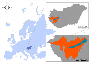
We selected the catchment area of Lake Balaton (Fig. 1) to study mapping of soil hydraulic properties, because it is an important area in Hungary from the point of modelling hydrological, ecological, and meteorological processes or planning land use and management. The size of the catchment is 5775 km². The mean depth of the lake is 3.5 m; therefore the water quality and quantity of the lake are sensitive to environmental changes. It has a warm temperate climate with 9–12 ^∘C mean annual temperature and 560–770 mm mean annual precipitation; lower temperature and higher rainfall values tend to be towards the western and elevated areas. Elevation is between 100 and 500 m on the northern part and 100 and 300 m in other areas of the catchment. The main soil types are Luvisols (53 %), Cambisols (18 %), Gleysols (10 %) and Histosols (5 %), and in addition to these Stagnosols, Arenosols, Regosols, Leptosols and Chernozems also occur (IUSS Working Group WRB, 2014).

Table 1 Available environmental covariates.

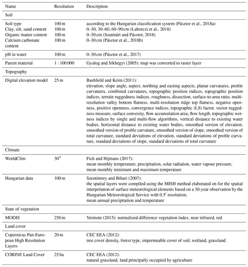
For the catchment spatial information on soil type, clay, silt and sand content, organic matter content, calcium carbonate content and pH in water (pH) at 100 m resolution were provided by the DOSoReMI.hu (Digital, Optimized Soil Related Maps and Information; Pásztor et al., 2018b) framework (Table 1). As soil chemical properties – organic matter content, calcium carbonate content and pH – were only available for the 0–30 cm depth, those could only be considered for the topsoil predictions. Information on topography, meteorology, geology and vegetation listed in Table 1 was used as predictors and environmental covariates for the elaboration of PTFs and direct mapping accordingly.

Topographical parameters were calculated with SAGA GIS tools (Conrad et al., 2015) based on the digital elevation model. For the mapping of soil hydraulic properties all covariates were harmonized, projected to the Hungarian Uniform National Projection system, rasterized if necessary and resampled to 100 m resolution.

2.2 Dataset to relate soil hydraulic properties and environmental information

For the prediction of soil hydraulic properties based on soil and other environmental variables the Hungarian Detailed Soil Hydrophysical Database (Makó et al., 2010) was used, extended with topographical, meteorological, geological information and remotely sensed vegetation properties (Table 1), called MARTHA version 3.0 (acronym of the Hungarian name of the dataset). MARTHA consists of 15 142 soil horizons' data belonging to 3970 soil profiles. The samples in it have measured information on basic soil properties – e.g. soil depth, organic matter content, clay, silt and sand content, calcium carbonate content and pH – and also on soil hydraulic properties such as soil water retention at different matric potential values.

2.3 Mapped soil hydraulic properties

We mapped soil water content at 0, −330 and −15,000 cm matric potential values, THS, FC and WP respectively, because these soil hydraulic properties are often required for various purposes. The definition of FC varies across different countries. In Hungary FC is determined at −330 cm matric potential; therefore water content at −100 or −200 cm was not analysed in the presented work.

The information on soil properties was available for 0–30, 30–60 and 60–90 cm soil depths, and this determined the vertical resolution of the soil hydraulic maps. As PTFs include depth as an independent variable, they are applicable for any soil depth intervals.

2.4 Methods for soil hydraulic properties mapping

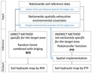
Soil hydraulic properties were mapped both with direct and indirect methods for the catchment of Lake Balaton. In direct mapping, the target soil variable is directly interpolated over the domain of interest, whereas in indirect mapping not the target variable but its components, factors and/or covariates are interpolated first, and then these interpolated surfaces are used to compute and map the target variable. In the direct method we used the geostatistical approach to spatial inference measured soil hydraulic data collected in profiles of the catchment through the modelling of their relationship with environmental covariates. In indirect mapping PTFs were derived first to describe relationships between soil hydraulic properties and easily available soil and other environmental parameters. In this approach the full national MARTHA database provided soil reference data, and nationwide, spatially exhaustive environmental auxiliary information was used. The PTF predictions were then spatially implemented on the environmental covariates clipped for the catchment area of Lake Balaton (Fig. 2).

Figure 2 Flowchart about the main steps of direct and indirect soil hydraulic mapping methods.

2.4.1 Pedotransfer-function-based indirect mapping (HUN-PTF)

We derived PTFs for THS, FC and WP using soil depth, soil properties and other environmental covariates listed in Table 1 as independent variables. Organic matter content, calcium carbonate content and pH could be considered only for the topsoil (0–30 cm) predictions, because those are not available for the subsoils on the Balaton catchment area.

For the construction of PTFs those samples were selected from MARTHA dataset which had measured values of soil horizons or layers considered dependent and independent variables. We needed two kinds of predictions: (1) for topsoils where we could include organic matter content, calcium carbonate content and pH among the predictors; and (2) for subsoils without the above soil chemical parameters, because those are not available for the 30–60 and 60–90 cm soil depths on the Balaton catchment. First we randomly selected 67 % of the samples from those which had data on the dependent and all the independent variables available on the catchment area to derive the PTFs. The remaining 33 % was used to compare the performance of the PTFs; this we called the TEST_CHEM set. In the second step we needed a training set (67 % of data) and a test set (33 % of data) also for subsoil prediction for which we did not have to apply the restriction on the soil chemical properties; therefore we could include more samples for the analysis. As a test set we used the samples of the TEST_CHEM set and further added cases to reach the 33 % of the complete data appropriate for subsoil predictions. Again the remaining 67 % was used for training.

The number of samples used to train and test the PTFs was 8157 and 12 039 for THS, 8051 and 11 931 for FC, and 8195 and 12 036 for WP, with and without soil chemical properties respectively.

We analysed the prediction performance of the two widely used machine learning algorithms, random forest (RF) of the R package “ranger” (Wright et al., 2018) and the generalized boosted regression model (GBM) of the R package “gbm” (Ridgeway, 2017), for the prediction of THS, FC and WP. The advantage of these two algorithms is that the prediction intervals of the dependent variable are computed as a function of the independent variables.

Both algorithms build ensembles of models from regression trees. In regression trees, data are recursively partitioned to increase homogeneity in the subsets; in this way the residual sum of squares is minimized (Breiman et al., 1984). The difference between GBM and RF is the way the forest is built from the individual trees. RF relies on averaging the result of the trees in the ensemble. The trees are grown on n_tree bootstrap samples of the training data independently from each other (Breiman, 2001); therefore it is a bagging type ensemble. At each split of the trees only a small set of predictors is selected randomly to analyse which variable at which split point is the best for the partition, i.e. minimize the sum of squares. In GBM the ensemble model is grown sequentially; at each iteration step the next model is built with respect to the error of the ensemble learnt so far (Friedman, 2001; Natekin and Knoll, 2013), which is characteristic for the boosting type ensemble, already included in its name (Dietterich, 2000). In each split all possible predictors are considered.

Optimization of the parameter set in the RF and GBM model was performed with the train function of the R package “caret” (Kuhn et al., 2018). A 5-fold cross validation repeated five times was used to evaluate the performance of different parameter sets. For RF, the number of input parameters selected randomly at each split – which is set under the “mtry” argument – was tuned. In the case of GBM, influence of interaction depth and shrinkage were analysed. In ranger, the RF default value is 500 for the number of trees that was used for both RF and GBM. Also for the minimum number of observations in the terminal nodes of the trees the default value of the algorithms was used. During the tuning of model parameters the importance of variables was calculated both for the GBM and RF methods to eliminate the less relevant predictors (Gregorutti et al., 2017; Nussbaum et al., 2018). Variable importance is the measure of relevance of each predictor; it is calculated from the average sum of squares improvements at each split, where the predictor was selected to partition the data (Hastie et al., 2009). A value of 100 is assigned to the largest variable importance value, and the others are scaled accordingly to provide relative measure. The most important 50–50 predictors out of 173 for topsoils and 170 for subsoils have been selected from both GBM and RF models. After concatenating the 50–50 most important variables, parameter tuning was performed again with the decreased number of predictors. We compared the accuracy of all models based on the cross-validation results and built the final prediction model (PTF) with the better performing and simpler algorithm on all training data with the optimized parameters. The performance of the PTFs was determined using the RMSE (Eq. 1) and coefficient of determination (R²; Eq. 2).

$$\begin{array}{}\text{(1)}& {\displaystyle }& {\displaystyle }\mathrm{RMSE}=\sqrt{{\displaystyle \frac{\mathrm{1}}{N}}\sum _{i=\mathrm{1}}^N{\left(y_i-{\widehat{y}}_i\right)}^{\mathrm{2}}}=\sqrt{\mathrm{MSE}}\text{(2)}& {\displaystyle }& {\displaystyle }{R}^{\mathrm{2}}=\mathrm{1}-{\displaystyle \frac{\sum _{i=\mathrm{1}}^N{\left(y_i-{\widehat{y}}_i\right)}^{\mathrm{2}}}{\sum _{i=\mathrm{1}}^N{\left(y_i-\stackrel{\mathrm{‾}}{y}\right)}^{\mathrm{2}}}}\end{array}$$

The performance of PTFs on the training dataset was based on the results of a 5-fold cross validation and out-of-bag samples – not included in the bootstrap sample used to build the tree – for GBM and RF respectively. In RF, the accuracy of out-of-bag samples was analysed. The uncertainty of the predictions was characterized with the 5 % and 95 % quantiles of the predicted values, calculated within the ranger and gbm packages during the derivation of the prediction algorithms.

HUN-PTFs derived on the MARTHA dataset were used to calculate the soil hydraulic properties (THS, FC, WP) based on the available soil and environmental covariates available for the catchment (Table 1, Sect. 2.1) as predictors; hence those were mapped indirectly. Soil information is currently available for the 0–30, 30–60 and 60–90 cm. The input information depth was set to 15, 45 and 75 cm for the first, second and third layer respectively during the calculation of soil hydraulic property maps.

We provided information on the uncertainty of the predictions by pixels. In addition to the median, the 5 % and 95 % quantiles of the predicted values were also mapped for each soil hydraulic property. The prediction intervals were calculated by the PTFs.

2.4.2 Direct mapping with the geostatistical method (RFK)

We applied random forest combined with kriging (RFK), which can be considered a new workhorse of digital soil mapping (Keskin and Grunwald, 2018). In the case of RFK, the deterministic component of spatial soil variation is modelled by the RF introduced above, whereas the stochastic part of variation is modelled by kriging using the derived residuals.

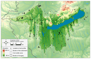
Figure 3 Location of soil profiles used for the geostatistical soil hydraulic mapping on the Balaton catchment study area. The solid line indicates the border of the catchment; the dashed line shows the area with the 5 km buffer zone.

Table 2 Description statistics of measured soil properties of the Balaton catchment.

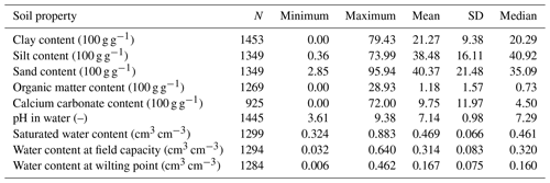
For the geostatistical analysis those samples of the MARTHA database which fall within the catchment plus a 5 km buffer zone area were selected. The buffer zone was used to increase the accuracy of geostatistical calculations also at the border of the catchment. On the study site data of 359 soil profiles are available from the MARTHA (Fig. 3). Table 2 summarizes the measured soil chemical, physical, hydraulic data of the soil profiles' horizons.

First of all, we harmonized the soil hydraulic dataset for the required soil depths (i.e. 0–30, 30–60, 60–90 cm) by using equal-area splines (Malone et al., 2009), and then we used RFK for predicting each soil hydraulic property for each soil depth, respectively. For RF, we also optimized the parameter set by the “train” function of the R package caret using a 5-fold cross validation repeated five times. The most important 50 covariates – out of 173 for topsoils and 170 for subsoils, listed in Table 1 – were selected, and the final RF model was optimized with those predictors. We used the final RF model for predicting the deterministic component. We computed the residuals, and then we estimated their variogram using Matheron's (1963) method-of-moments estimator. An isotropic variogram model was fitted to the estimated variogram by the “fit. variogram” function of the R package “gstat” (Gräler et al., 2016; Pebesma, 2004). We kriged the residuals and then we added them to the deterministic component predicted by RF. The above-described modelling procedure was applied for each soil hydraulic property and for each soil depth. The performance of RF was described with RMSE (Eq. 1) and R² (Eq. 2).

2.4.3 Evaluating the performance of soil hydraulic maps

The performance of soil hydraulic maps was evaluated based on observed soil hydraulic properties harmonized for 0–30, 30–60 and 60–90 cm depth with the method described in Sect. 2.4.2. RMSE and mean square error skill score (SS_mse) (Nussbaum et al., 2018) Eqs. (1–3) were calculated for each map.

$$\begin{array}{}\text{(3)}& {\displaystyle }{\mathrm{SS}}_{\mathrm{mse}}=\mathrm{1}-{\displaystyle \frac{\sum _{i=\mathrm{1}}^N{\left(y_i-{\widehat{y}}_i\right)}^{\mathrm{2}}}{\sum _{i=\mathrm{1}}^N{\left(y_i-\frac{\mathrm{1}}{N}\sum _{i=\mathrm{1}}^N{y}_i\right)}^{\mathrm{2}}}}\end{array}$$

The performance of soil hydraulic maps derived with HUN-PTFs and RFK was compared to the 3-D European soil hydraulic maps (EU-SoilHydroGrids v1.0) (Tóth et al., 2017). In EU-SoilHydroGrids the input information for mapping was SoilGrids 250 m (Hengl et al., 2017), on which EU-PTFs (Tóth et al., 2015) were applied; hence its resolution is 250 m. We converted the information of EU-SoilHydroGrids to 0–30, 30–60 and 60–90 cm to be able to compare its performance to the 100 m resolution new soil hydraulic maps derived by HUN-PTFs and RFK.

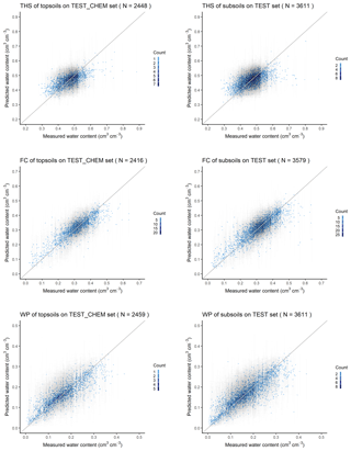
Figure 4 The scatter plot of the measured versus predicted water retention values with 90 % prediction interval on test datasets based on the random forest method. THS: saturated water content, FC: water content at field capacity, WP: water content at wilting point, TEST_CHEM set: test dataset in which chemical soil properties are available for the predictions, and TEST set: test dataset in which chemical soil properties are not necessarily available for the predictions.

The Kruskal–Wallis test implemented in the R package “agricolae” (De Mendiburu, 2017) was applied at the 5 % significance level on the mean-square-error values for the comparison of the PTFs with different input variables and also the soil hydraulic maps derived using different methods.

All statistical analyses were performed in R (R Core Team, 2018).

3 Results and discussion

3.1 Pedotransfer functions

During the parameter tuning of RF and GBM we found that decreasing the number of input variables – from 173 to 69–76 and from 170 to 65–77 in the case of topsoil and subsoil predictions respectively – significantly improved the prediction of top- and subsoil FC and subsoil WP. Although differences between RMSE values were less than 0.0001 cm³ cm⁻³, these are negligible from a practical point of view. In Nussbaum et al. (2018) the number of input parameters were decreased from 300–500 environmental covariates to the 10, 20, 30, 40 and 50 most important ones. No changes in performance were found during validation. We can assume that the performance of predictions will neither increase nor decrease if more important independent variables are used exclusively for the predictions. However, the selection of the most important independent variables can reduce (i) the unnecessarily large size of the model, which can speed up mapping of soil hydraulic properties for larger areas at fine resolution; and (ii) multicollinearity between predictor variables. Dorman et al. (2013) extensively studied the problem of collinearity to test its impact on predictions of ecological parameters. They analysed multiple regression and machine learning methods and found that prediction performance of random forest did not get worse due to high collinearity in the training dataset even when the structure of collinearity was different in training and validation data. The influence of multicollinearity on the prediction performance is partly reduced due to the random selection features of RF but could be further elaborated on in the presented methods; however, this was beyond the scope of the presented work.

In the case of RF, the optimal number of input parameters randomly selected at each split was between 10 and 20, depending on soil hydraulic parameter. In GBM optimal interaction depth varied between 20 and 40. The iteration converged during the prediction of lower 5 % and upper 95 % quantiles but did not for 50 %, which is the most probable predicted value. Therefore, the influence of shrinkage and increasing the number of trees to 1000 was also analysed but only in the prediction of FC because training with low shrinkage values is very time-consuming. We tuned shrinkage to 0.1 and 0.01 with both 500 and 1000 trees, setting the interaction depth to 4, 6 and 10. Shrinkage with a 0.1 value was more accurate than with 0.01, independent from the number of trees, and increasing the number of trees did not significantly improve the prediction; therefore shrinkage was set to 0.1 and the default 500 number of trees were used in the algorithm.

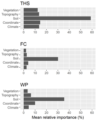
Figure 5 Mean relative importance of covariates used to predict soil hydraulic properties based on random forest analysis on the training set of the MARTHA database. THS: saturated water content, FC: water content at field capacity, and WP: water content at wilting point.

Table 3 The performance of hydraulic PTFs on training and test datasets. THS: saturated water content, FC: field capacity, WP: wilting point, RF: random forest method, GBM: generalized boosted regression method, TEST_CHEM set: test dataset in which chemical soil properties are available for the predictions, TEST set: test dataset in which chemical soil properties are not necessarily available for the predictions, RMSE: root mean square error, and R²: determination coefficient.

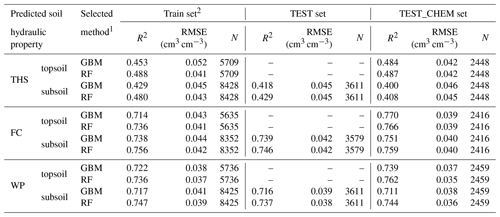
¹ Input parameters included in all analyses for topsoils: soil type according to the Hungarian classification system, sand (50–2000 µm), silt (2–50 µm) and clay content (<2 µm) (100 g g⁻¹), mean depth (cm) and information on topography, vegetation, meteorology and parent material listed in Table 1. For subsoils organic matter content (100 g g⁻¹), pH in water and calcium carbonate content (100 g g⁻¹) were included as well. ² Prediction error calculated on training is based on the out-of-bag error in the case of RF and 5-fold cross validation in the case of the GBM method.

The performance of PTFs derived by RF and GBM on training and test sets is included in Table 3. In the case of all soil hydraulic properties RF performed significantly better than GBM based on MSE on TEST and TEST_CHEM sets both for topsoil and subsoil predictions, except for WP topsoil predictions, where there was no significant difference between the methods. In this way PTFs derived with the RF method were selected for mapping soil hydraulic properties. RMSE values calculated on the test sets for RF were between 0.042 and 0.045 cm³ cm⁻³ for THS, 0.039 and 0.042 cm³ cm⁻³ for FC, and 0.035 and 0.038 cm³ cm⁻³ for WP, which is close to the performance of other internationally accepted PTFs (e.g. Botula et al., 2013; Román Dobarco et al., 2019; Zhang and Schaap, 2017). R² was 0.408–0.487, 0.746–0.766 and 0.737–0.762 for THS, FC and WP respectively on test sets in the case of RF. Figure 4 shows the scatterplots of measured versus predicted values with the 90 % prediction interval. At the lower end of the soil hydraulic property distribution, real values were closer to the lower 5 % quantile predictions; at the higher end of its distribution, the real values are closer to the upper 95 % quantile predictions. When we compared the performance of RF derived for topsoils – which includes organic matter content, pH and calcium carbonate content as well among the input parameters – and subsoils, there was no significant difference based on the results in the TEST_CHEM set. This is due to their correlation with other environmental predictors considered in the PTFs such as soil texture, depth, longitude, elevation, slope angle, multi-resolution valley bottom flatness, horizontal distance to existing water bodies, roughness, temperature, precipitation, solar radiance, spectral reflectance in red and near infrared, and normalized difference vegetation index (Adhikari et al., 2014; Hengl et al., 2017; Nussbaum et al., 2018). When other environmental covariates than soil-related variables are not included among input parameters, chemical properties significantly improve prediction (Hodnett and Tomasella, 2002; Khodaverdiloo et al., 2011; Tóth et al., 2015). In the case of the THS range, the predicted values using chemical parameters as well were closer to the range of measured values; therefore we also considered soil chemical properties for the topsoil predictions. For FC and WP, the range of values predicted with PTF not including chemical variables were closer to that of measured values; hence information on organic matter content, pH and calcium carbonate content – even though it is available – was not considered during the estimation of topsoil hydraulic properties.

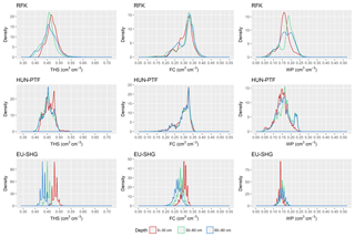
Figure 6 Density plots of mapped soil hydraulic values by mapping methods and depth. THS: saturated water content, FC: water content at field capacity, WP: water content at wilting point, RFK: derived by random forest with kriging, HUN-PTF: calculated with Hungarian pedotransfer functions, and EU-SHG: values from the EU-SoilHydroGrids 250 m dataset.

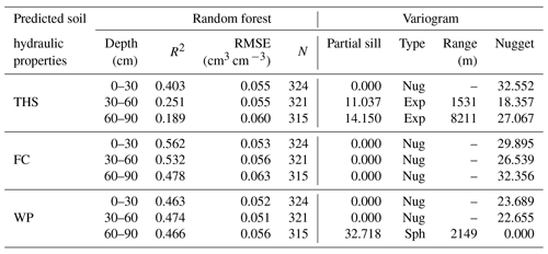
Table 4 The performance of the random forest method and parameters of the fitted variogram models during the geostatistical mapping approach.

The presented PTFs were derived on the full MARTHA dataset; therefore those are applicable to predict the THS, FC and WP of soils in the whole Pannonian region.

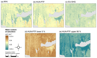
Figure 7 Map of water content at saturation in 0–30 cm soil depth derived by the random forest and kriging mapping approach (RFK) (a), Hungarian pedotransfer functions (HUN-PTF) (b), and cut from the EU-SoilHydroGrids 250 m dataset (EU-SHG) (c), as well as possible lower 5 % (d) and upper 95 % (e) quantiles based on HUN-PTF for a section of the Balaton catchment.

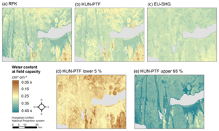
Figure 8 Map of water content at field capacity in 0–30 cm soil depth derived by the random forest and kriging mapping approach (RFK) (a), Hungarian pedotransfer functions (HUN-PTF) (b), and cut from the EU-SoilHydroGrids 250 m dataset (EU-SHG) (c), as well as possible lower 5 % (d) and upper 95 % (e) quantiles based on HUN-PTF for a section of the Balaton catchment.

3.1.1 Importance of independent variables

For THS, organic matter content, silt, sand content, pH, clay and calcium carbonate content are the most important variables with a relative importance of over 20 % based on the final RF model. In addition to those properties, soil depth, mean annual precipitation, mean monthly maximum, minimum and mean temperature of some months, mean monthly radiation, longitude, horizontal and vertical distance to existing water bodies, multi-resolution valley bottom flatness and ridge top flatness, water vapour pressure in August and spectral reflectance in the near infrared are among the most important 30 variables, having 10 %–15 % relative importance. For FC and WP, clay, silt, and sand content and organic matter content are the most important variables, having a relative importance around and over 20 %. Soil type, mean monthly precipitation in July, vertical distance to existing water bodies and longitude have a relative importance around 5 %–14 % in the case of FC. All the other environmental covariates have a relative importance of less than 5 %. For WP, longitude, mean monthly precipitation of November and July, elevation, vertical and horizontal distance to existing water bodies, calcium carbonate content, mean monthly radiation, pH, depth, mean monthly water vapour pressure, multi-resolution ridge top flatness and spectral reflectance in the near infrared have a relative importance of between 5 % and 16 %. Information on topography was found to be important for the prediction of soil hydraulic properties by Obi et al. (2014), Rawls and Pachepsky (2002), Romano and Chirico (2004), and Zhao et al. (2016) as well. Information on land cover was not retained after selecting the most important variables.

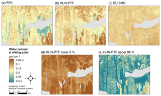
Figure 9 Map of water content at wilting point in 0–30 cm soil depth derived by the random forest and kriging mapping approach (RFK) (a), Hungarian pedotransfer functions (HUN-PTF) (b), and cut from the EU-SoilHydroGrids 250 m dataset (EU-SHG) (c), as well as possible lower 5 % (d) and upper 95 % (e) quantiles based on HUN-PTF for a section of the Balaton catchment.

When soil chemical properties (organic matter content, calcium carbonate content, pH) are not included among input parameters, sand, silt and clay content are by far the most important three independent variables (39 %–100 %). In the case of THS, depth also has a higher relative importance (52 %). For the prediction of FC, the importance of soil type increases to 18 %. In WP prediction there is no notable change in variable importance when chemical properties are not included in the RF.

The summary of the variable importance analysis showed that soil properties are by far the most important input parameters for the prediction of soil hydraulic properties (Fig. 5). In this way resolution of soil maps determined the resolution of the derived soil hydraulic maps, which was 100 m.

Figure 10 Differences between possible lower 5 % and upper 95 % water content at saturation (a), field capacity (b), and wilting point (c) in 0–30 cm soil depth for a section of the Balaton catchment.

3.2 Random forest combined with kriging (RFK)

During the RF parameter tuning we also found that decreasing the number of environmental covariates – from 173 to 50 and from 170 to 50 in the case of topsoil and subsoil respectively – significantly improved the prediction accuracy for each soil hydraulic property. For the final RF models the optimal number of randomly selected predictors at each split varied between 5 and 40 depending on the given soil hydraulic property. The performance of the final RF models is summarized in Table 4. R² varies between 0.189–0.403, 0.478–0.562 and 0.463–474 for THS, FC and WP, respectively. RMSE was 0.055–0.060, 0.053–0.063 and 0.051–0.056 for THS, FC and WP, respectively. For describing spatial variation of the soil hydraulic properties the most important environmental covariates were the soil type, organic matter content (for topsoil), clay, silt and sand content and the pH (for topsoil). The final RF models were used for estimating the deterministic component for each soil hydraulic property.

The parameters of the fitted variogram models are summarized in Table 4. In the case of exploratory variography, most of the experimental variograms did not show spatial structure, and the applied variogram fitting algorithm was not able to find a satisfactory variogram model in the case of six out of nine maps in 200 iterations. Hence, a nugget model was fitted to those variograms (Table 4), which is not rare in digital soil mapping (Hengl et al., 2015; Szatmári and Pásztor, 2018; Vaysse and Lagacherie, 2017). In Table 4 we have observed that the lower the R² value was, the higher the range parameter became. The fitted variogram models were used for kriging of the RF residuals for each soil hydraulic property. We summed the RF predictions and the kriged residuals to get the RFK maps for each of the target hydraulic properties.

Table 5 The performance of soil hydraulic maps derived by the random forest and kriging method (RFK), Hungarian pedotransfer functions (HUN-PTF) and from the EU-SoilHydroGrids 250 m dataset (EU-SHG) on the Balaton catchment. RMSE: root mean square error and SS_mse: mean square error skill score.

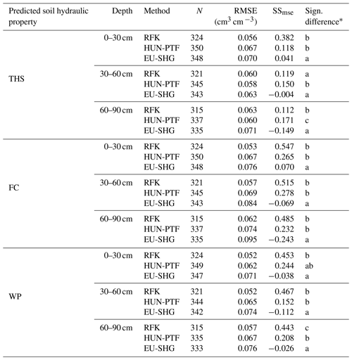
^∗ Different letters indicate significant differences at the 0.05 level between the accuracy of the methods based on the squared error; for example performance indicated with the letter c is significantly better than the one noted with letters b and a.

3.3 Performance of soil hydraulic maps

New 100 m resolution soil hydraulic maps significantly outperformed the EU-SoilHydroGrids (Table 5), which was expected because (i) reference soil data originate from the mapped area and also (ii) spatially denser and (iii) locally trained models are used. In addition, several environmental covariates were considered for the predictions and relationship between easily available soil properties, and soil hydraulic parameters were derived from local data.

In the case of mapping six out of nine soil hydraulic maps, there was no significant difference between maps derived by RFK and HUN-PTFs. In the case of THS, HUN-PTF performed significantly better for mapping the 30–60 and 60–90 cm. For calculating WP at 60–90 cm soil depth RFK, was significantly better than the HUN-PTF method.

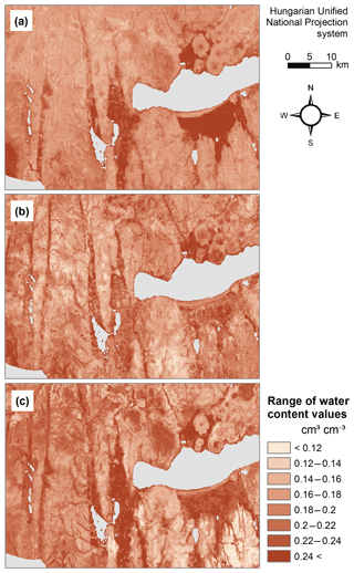
The range of predicted values is smaller in the case of the HUN-PTF method than in RFK, which is due to the averaging approach of the algorithm which in the case of RFK is spatially corrected, allowing a wider range in the predicted values (Figs. 6, 7, 8, 9). Density plots of predicted values are smoother in the case of RFK than in HUN-PTF and EU-SoilHydroGrids maps (Fig. 6). This is due to adding residuals of kriging, which modifies the values derived by random forest. In EU-SoilHydroGrids soil hydraulic values were calculated with linear regression based on soil properties available from SoilGrids, where mapping was performed with RF without kriging. In this way possible soil input combinations are limited in the European maps. In the SoilGrids, algorithms are derived from a global dataset (Hengl et al., 2017), which has sparser measured data than the Hungarian soil profile database used to map soil properties (Laborczi et al., 2018; Szatmári and Pásztor, 2018). In addition, RF is based on an averaging algorithm, which limits the ability to describe local extreme values. These result in a smaller range and variability of calculated soil hydraulic properties on EU-SoilHydroGrids maps than on RFK or HUN-PTF ones (Fig. 6) The basic Hungarian soil maps were derived with regression kriging methods, thus providing smoother soil input data for the calculations. As an example of how differences in the range of predicted soil hydraulic properties can be visualized, the maps of THS, FC and WP are shown on Figs. 7–9a, b and c for a selected area of the catchment. Differences between the new and already available maps also occur due to the differences in resolution, which are 100 m for RFK and HUN-PTF and 250 m for EU-SoilHydroGrids. Even though the influence of topographical information was less than that of soil properties when PTFs were derived, the pattern of topography is visible on the maps derived by RFK and HUN-PTFs. This is due to the soil layers used as inputs for calculating the soil hydraulic properties, because topographical information was important among the covariates when the maps on them were derived (Szatmári et al., 2013). In RFK, the influence of the topography is less visible; it could be smoothed by adding kriged residuals. A map of possible lower 5 % and upper 95 % values based on the HUN-PTF method is also shown in Figs. 7–9d and e. The range between the lower and upper possible values (Fig. 10) is usually higher for Histosols, Gleysols and Luvisols under forest land use, because these kinds of soils are underrepresented in the MARTHA database.

Although we compared the performance of the new soil hydraulic maps to that of EU-SoilHydroGrids, differentiating the uncertainty of the maps originating from the soil input layers – i.e. DOSoReMI.hu and SoilGrids – was out of the scope of our study.

Table 6 Proportion of mapped area having smaller than 0.025, 0.025–0.050, 0.050–0.100 and bigger than 0.100 cm³ cm⁻³ absolute difference between predicted soil hydraulic values derived by the geostatistical method (RFK) and applying pedotransfer functions on local soil and environmental covariates (HUN-PTF).

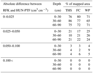
The average difference between the RFK and HUN-PTFs maps is between 0.003 and 0.012 cm³ cm⁻³ for THS, 0.011 and 0.015 cm³ cm⁻³ for FC, and 0.015 and 0.018 cm³ cm⁻³ for WP, depending on soil depth. The absolute difference between the maps derived with HUN-PTFs and RFK is less than 0.025 cm³ cm⁻³ for at least 65 % of the mapped area and was always smaller than 0.100 cm³ cm⁻³ (Table 6). On those areas where the difference between RFK and HUN-PTF was higher than 0.025 cm³ cm⁻³, HUN-PTF predicted lower water retention at all matric potential values for Histosols and Luvisols under forest land use type. WP values predicted with HUN-PTFs were higher than that of RFK for Luvisols with sandy texture and under forest land use type.

Based on SS_mse values in the case of seven out of nine soil hydraulic maps, the RFK mapping method was more accurate than HUN-PTF, although only the calculation of WP in 60–90 cm depth was significantly better. For THS, HUN-PTFs performed significantly better at 30–60 and 60–90 cm soil depth.

In this study priority was placed on the usability and transferability of the results into practical applications. The purpose of the presented research was to derive as accurate maps as possible. Thus ability for full comparability of the methods did not determine the design of the methodology and statistical analysis. Therefore, in the RFK analysis all measured data were used for the mapping. For the PTF approach, predictions were tested on randomly selected 33 % samples of the whole MARTHA database without distinguishing samples located on the catchment, as it is usually done in deriving PTFs. This provides broader information and possibility for a wider application of PTFs. The presented HUN-PTF mapping method can be applied in any catchments of Hungary.

Table 7 Differences between pedotransfer-function-based (PTF) and geostatistical (RFK) mapping methods based on calculating saturated water content, field capacity and wilting point for the Balaton catchment.

3.4 Practical use of the analysis

RF performed significantly better than GBM in seven cases out of eight on test sets. RF was found to be a suitable method to provide information on the prediction uncertainty; any desired quantiles of the predicted value can be calculated. This enables it to include extreme soil hydraulic parameters for hydrological simulations. Its further advantage is that it can handle several independent variables; the performance of prediction is not influenced by multicollinearity between independent variables and the inclusion of unimportant input parameters. Calculation on multiple cores is implemented in the random forest algorithm in the ranger R package, which can significantly decrease computation time.

Easily available soil properties such as sand, silt and clay content; organic matter content; and depth were the most important input variables for the calculation of THS, FC and WP among the analysed 173 soil and environmental covariates. For THS, calcium carbonate content and pH were also among the independent variables with higher importance. Geographical coordinates, information on topography, climate and vegetation had a smaller relative importance. Covariates on land use and parent material were not among the 50 most important variables. Therefore, the resolution of available soil maps determined the resolution of new soil hydraulic maps, which is 100 m.

The number of input variables can be decreased based on variable importance, which can significantly decrease computation time, and information not relevant for the prediction can be discarded. For practical application it is desirable to decrease the size of the prediction models when PTFs are applied for soil hydraulic mapping at the country scale at finer resolution.

If data on topography, climate and vegetation are also considered for the prediction, missing information on chemical properties, such as organic matter content, pH and calcium carbonate content, can be covered by the environmental covariates without significant loss of performance.

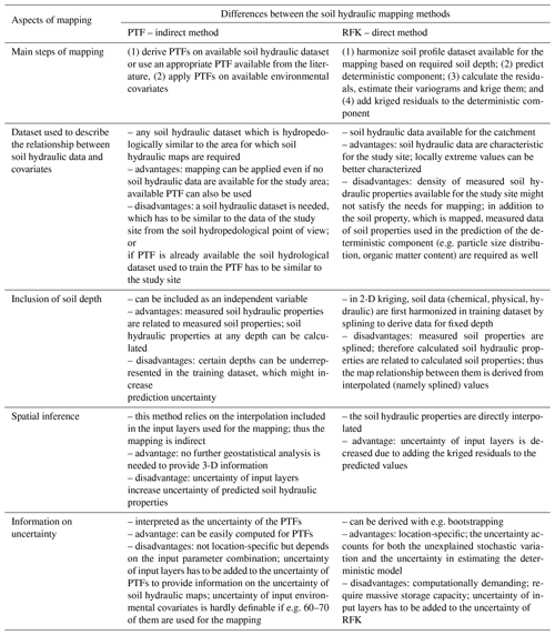
HUN-PTFs performed significantly better for the prediction of THS at 30–60 and 60–90 cm depth, although the absolute difference between the RFK and HUN-PTFs maps is less than 0.025 cm³ cm⁻³ for at least 75 % of the area. Spatial patterns of topography are less dominant on the soil hydraulic maps prepared by the RFK method due to kriging the residuals, which is an advantage. Maps prepared by the HUN-PTFs cannot decrease the influence of topography included in the input layers, even if topographical parameters are not important for the prediction of soil hydraulic properties that are visible on the soil hydraulic maps. Considering all these results we suggest using the soil hydraulic maps prepared by the RFK only if the most probable soil hydraulic value is needed for the Balaton catchment area. Information on the uncertainty of the predicted values can be derived with geostatistical methods as well; for example Szatmári and Pásztor (2018), Rudiyanto et al. (2016), Viscarra Rossel et al. (2015) presented possible methods. According to Szatmári and Pásztor (2018), quantile-regression-forest-based (Meinshausen, 2006) uncertainty quantification outperforms most of the prediction techniques used in digital soil mapping. Furthermore, they have pointed out that bootstrapping-based uncertainty quantification for RFK is quite time-consuming, as well as requiring massive storage and computing capacity. The ranger package – with which we derived the HUN-PTFs – includes the implementation of quantile regression forest (Meinshausen, 2006) for the calculations of the prediction intervals. If information on uncertainty is needed as well, the use of maps derived by the HUN-PTFs is recommended. In Table 7 we highlight the most important differences between pedotransfer-function-based (HUN-PTF) and geostatistical (RFK) soil hydraulic mapping based on the Balaton catchment. Most of the findings are in line with Hengl et al. (2018b), Tranter et al. (2009), Vaysse and Lagacherie (2017), and Webster and Oliver (2007).

4 Conclusions

Based on results of six out of nine soil hydraulic maps there is no significant difference in performance between the pedotransfer function (indirect) and geostatistical (direct) method on the Balaton catchment area. The benefit of maps computed with random forest and kriging is that locally extreme values can be characterized better. In the case of pedotransfer-function-based mapping, it is advantageous that the calculation of uncertainty is much less computationally intensive than it is with geostatistical methods, although it would be interesting in the future to analyse the difference between uncertainty maps calculated with the different methods, specifically for soil hydraulic properties.