the Creative Commons Attribution 4.0 License.
the Creative Commons Attribution 4.0 License.
 | 05 Jun 2019
Observation operators for assimilation of satellite observations in fluvial inundation forecasting
Sarah L. Dance
Javier García-Pintado
Nancy K. Nichols
Polly J. Smith
Images from satellite-based synthetic aperture radar (SAR) instruments contain large amounts of information about the position of floodwater during a river flood event. This observational information typically covers a large spatial area but is only relevant for a short time if water levels are changing rapidly. Data assimilation allows us to combine valuable SAR-derived observed information with continuous predictions from a computational hydrodynamic model and thus to produce a better forecast than using the model alone. In order to use observations in this way, a suitable observation operator is required. In this paper we show that different types of observation operators can produce very different corrections to predicted water levels; this impacts the quality of the forecast produced. We discuss the physical mechanisms by which different observation operators update modelled water levels and introduce a novel observation operator for inundation forecasting. The performance of the new operator is compared in synthetic experiments with that of two more conventional approaches. The conventional approaches both use observations of water levels derived from SAR to correct model predictions. Our new operator is instead designed to use backscatter values from SAR instruments as observations; such an approach has not been used before in an ensemble Kalman filtering framework. Direct use of backscatter observations opens up the possibility of using more information from each SAR image and could potentially speed up the time taken to produce observations needed to update model predictions. We compare the strengths and weaknesses of the three different approaches with reference to the physical mechanisms with which each of the observation operators allow data assimilation to update water levels in synthetic twin experiments in an idealised domain.
- Article
(1870 KB) - Full-text XML
- BibTeX
- EndNote


During a fluvial flood it is possible to use a numerical hydrodynamic model to predict future water levels and flood extents. Such predictions are subject to uncertainties and can be inaccurate; data assimilation can therefore be used to improve predictions by updating model forecasts based on various types of observations (e.g. Lai and Monnier, 2009; Matgen et al., 2007; Garcia-Pintado et al., 2013, 2015; Ricci et al., 2011; Barthélémy et al., 2016; Schumann et al., 2009; Oubanas, 2018; Oubanas et al., 2018a, b). For flooding, useful observations of the river flow rate or water depth could come from river gauges. However the number of gauges is declining worldwide (Vörösmarty et al., 2001), and a method that can work in ungauged catchments is therefore desirable. For this reason satellite images, and in particular synthetic aperture radar (SAR) images of flooded areas, can be a good source of information (Grimaldi et al., 2016).
SAR sensors are active, side-looking sensors included on several satellites, e.g. COSMO-SkyMed and Sentinel-1. Radiation (of wavelength cm to m), is emitted from the satellite and directed towards the surface of the Earth. The returning signal is recorded at a sensor and can be used to reconstruct information about the observed terrain. SAR radiation is cloud penetrating, giving the instruments all-weather capability. SAR instruments can also produce observations day and night, unlike passive sensors that rely on solar radiation.
The strength of the returned signal measured at the SAR sensor depends strongly on the roughness properties of the surface from which it has been reflected. During a flood event SAR images therefore generally show a clear difference between flooded and non-flooded areas. Pixels in flooded or other wet areas such as lakes and rivers have low backscatter values and appear as dark areas on SAR images; dry areas have higher backscatter values, and dry pixels therefore appear paler. There are a number of techniques for separating pixels into wet and dry areas based on backscatter. Methods include thresholding (e.g. Henry et al., 2006) with varying levels of user interpretation (as compared in Brown et al., 2016), region growing and clustering (“snakes”; e.g. Horritt et al., 2001), and change detection (e.g. Hostache et al., 2012). These techniques can be used to provide observational information for data assimilation frameworks but are also used for flood mapping and monitoring (as in, for example, Brown et al., 2016; Matgen et al., 2011) and for validation and calibration of inundation models (e.g. Mason et al., 2009; Baldassarre et al., 2009; Wood et al., 2016). In the case of model calibration, Mason et al. (2009) and Stephens et al. (2013) suggest that comparing modelled and observed derived water level measures from SAR images results in better calibration than when using binary wet–dry comparisons. However, it is not clear whether derived water levels provide better observation impact than wet–dry observations in data assimilation.
In this work we consider different ways in which information from an SAR image can be used to correct inundation forecasts using data assimilation. The use of observations requires two steps. First, we must extract relevant, useable information from an SAR image. This involves processing the raw SAR data in some way to produce an observation, or set of observations, per image. In the second step we need to use an observation operator to map our model state vector into observation space – i.e. we extract the equivalent information from our model in order to compare it to the observations. The size of the difference between the observation and the equivalent information from the model forecast is then used to calculate an update or correction to the forecast. The observation operator depends on the type of observational information used, and we show in this paper that the impact of observations on the forecast can be strongly dependent on the observation operator approach used. Despite this, the mechanisms through which different observation types and different observation operators update hydrodynamic forecasts have not received much attention in the literature.
In order to extract observational information from an SAR image, authors such as Mason et al. (2012), Giustarini et al. (2011), Neal et al. (2009) and Matgen et al. (2007) have used an approach which relies on identifying the flood edge. Terrain information, e.g. that from a digital terrain model, is then used to infer information about water levels on the floodplain. Water level observations (WLOs) can then be compared with model forecast water levels. Examples of two observation operators using flood-edge WLOs are described further in Sect. 3. A different type of observation is used for data assimilation in Wood (2016) and Hostache et al. (2018), in which flood probability maps are produced from SAR images using the method in Giustarini et al. (2016). Particle filter data assimilation techniques are then used to update a hydrodynamic model using flood probability maps as observations.
We propose a new type of observation operator which directly uses pixel-by-pixel backscatter values as observations. As in Wood (2016) and Giustarini et al. (2016), we rely on the fact that SAR images yield distinct distributions of wet and dry backscatter values. However, our method employs an ensemble transform Kalman filter (ETKF) approach with a novel observation operator; we directly use measured SAR backscatter values as observations rather than derived flood probability measures.
In this paper we examine the performance of our new observation operator and that of two flood-edge observation operators in a series of synthetic experiments. We compare the physical mechanisms by which the different approaches update predicted water levels in the ETKF; to the authors' knowledge these physical mechanisms have not been discussed in the literature before. We outline the ETKF data assimilation algorithm in Sects. 2 and 3; we describe the three observation operators which we have compared. Further details of our experiments are given in Sect. 4, including an outline of the hydrodynamic model. In Sect. 5 we demonstrate how well the assimilation can update model forecast water levels towards the truth with each observation operator and explore the different physical mechanisms by which updates are made. We also test the ability of the three operators to successfully update the model channel friction parameter through an augmented state vector approach. We find that our new backscatter operator generates better corrections to the state and parameter values than the simplest approach to assimilating flood-edge observations but does not always perform as well as the nearest wet pixel approach. In Sect. 6 we discuss issues relating to the application of our new observation operator to real data. In Sect. 7 we conclude with a comparison of the relative strengths and weaknesses of the three different observation operators.
In this paper we explore the use of observations from SAR images in updating forecasts from a hydrodynamic flood model. In Sect. 2.1 we outline the ETKF data assimilation framework we use in our experiments (Bishop et al., 2001), following the approach of Garcia-Pintado et al. (2013, 2015) and Cooper et al. (2018). In Sect. 2.2 we describe the joint state–parameter estimation method that we use to update the channel friction parameter value.
2.1 Ensemble transform Kalman filter (ETKF)
In data assimilation, forecasts from a numerical model are combined with observations of the same system. We use a state vector, x(tk)∈RN, to represent the state of the dynamical system at time tk. Here, our model domain is split into N computational cells, and the state vector contains N water depths at a given time. In this paper we use an ensemble of state vectors, where each state vector in the ensemble represents a possible state of the system. For an ensemble made up of M state vectors (members), xi, (), the best estimate of the true state of the system is represented by the mean state, , where
We can define a perturbation matrix, , that can be used to derive a measure of uncertainty in the mean state. The perturbation matrix is
We can then express the ensemble error covariance matrix, , as
The ETKF is a two-step sequential data assimilation technique. In the forecast step, each vector, xi, is evolved in time using the forecast equation,
where 𝔐 is the forecast model. Here, 𝔐 is a hydrodynamic model built using Clawpack code (see Sect. 4.1); the model evolves water levels in each ensemble member with time, generating an ensemble of flood forecast realisations.
In the update step the mean state vector and the error covariance matrix are both updated based on observational information. We use the ETKF in its standard application as a sequential filter. As such we perform an update step at the time of each available observation. We assume that the observations are related to the true state of the system, xt, according to
where the vector yobs∈Rp contains p observations. The vector ϵ represents observation error, which we assumed to be unbiased and stochastic with covariance . The observation operator, , maps the state vector into observation space. If the state vector and the observation vector contain the same quantity (e.g. water depth), then the observation operator is generally just required to pick out the values in the state vector corresponding to the spatial position of the observation or observations; this may involve spatial interpolation if observations are not located at model grid points. However, it is commonly the case that observations are different quantities to those in the state vector, and the observation operator therefore contains information about how the observed and state vector quantities are related as well as positional information. Different observation types (e.g. water elevation or wet–dry pixel information) therefore require different observation operators for the same model (i.e. for the same state vector).
In order to update the model forecast, it is useful to create a forecast–observation ensemble, which contains M forecast–observation vectors, , (), such that
Equation (6) shows that the observation operator, h, is applied to each state vector in order to extract observation-equivalent information; each forecast–observation vector, , is what would be observed if the corresponding state vector, , represented the true state of the system. The model equivalent of the observation vector is given by the mean of the forecast–observation ensemble, , where
Note that when the observation operator is non-linear,
We can also define a perturbation matrix for the forecast–observation ensemble matrix:
The mean state vector and error perturbation matrix are updated separately in the ETKF. The mean state is updated according to
where and are the means of the analysis and forecast ensemble respectively. The ETKF uses an ensemble version of the Kalman gain, , as defined in Eq. (13). The ensemble Kalman update Eq. (10) can be written in terms of the innovation, δy, where
The innovation is calculated in observation space. The term,
is known as the increment and is the difference between and . The increment is calculated in state space.
We use a square root formulation for the ETKF, following Ott et al. (2004), Livings et al. (2008) and Livings (2005). This formulation is also used in Garcia-Pintado et al. (2013) and Cooper et al. (2018). In this approach the ensemble version of K is written as
The state error perturbation matrix is updated in the ETKF according to
The perturbation matrix is updated by the matrix . We use an unbiased, symmetric square root formulation of the matrix T, constructed in a way that ensures that the analysis state error covariance, Pa=Xa(Xa)T, is the same as the analysis error covariance calculated in the Kalman covariance update (in, for example, Kalman, 1960). The formulation makes use of a singular value decomposition (Golub and Van Loan, 1996),
where and are orthogonal. The columns of U and V are the left and right singular vectors of respectively. The diagonal elements of the matrix are the singular values of . A solution for T is then
where I is the identity matrix. See Livings et al. (2008) and Cooper et al. (2018) for further details of how T is computed.
2.2 Joint state–parameter estimation
State augmentation techniques can be used to correct values of uncertain forecast model parameters at the same time as the state is updated. In this approach, parameters are appended to the state vector (see Smith et al., 2013, 2009, 2011; Navon, 1998; Evensen et al., 1998), producing an augmented state vector, xaug:
where . The vector b∈Rq contains q parameters. In this paper only one parameter is being updated, so that b is scalar. The parameter we are updating in this paper is the Manning's friction coefficient in the river channel, nch, as the evolution of a flood is known to be very sensitive to this parameter.
The forecast equation for the case of an augmented state vector can be written as
Equation (18) shows that we assume that the value of nch remains constant during the forecast step and changes only when the update equation is applied.
The augmented state vector is updated by the ETKF algorithm through Eqs. (10) and (14). Parameter values are updated according to the observations due to covariances between errors in the model state and errors in the parameters.
Model friction parameter values are more traditionally calculated using offline calibration techniques and data from previous flood events. Updating parameter values using a state augmentation approach has the advantage that it uses information from observations of the flood event of interest as it occurs. State augmentation can therefore take into account any recent changes to the river and its environment.
Much existing work on data assimilation for fluvial inundation forecasting has focussed on assimilating derived water level observations. Water level extraction is based on the fact that it is usually possible to differentiate between wet and dry areas in an SAR image; the contrast in backscatter between wet and dry pixels means that it is therefore possible to determine the position of the edge of a flooded area. Along this edge, the water elevation is the same as the elevation of the topography. This means that as long as a flood edge can be accurately identified and topographical information is available (e.g. a digital terrain model – DTM), water levels at the flood edge can be derived from an SAR image. This approach has also been used for operational flood mapping, e.g. in Brown et al. (2016). In practice, it is not possible to accurately determine flood extents from SAR images over the whole “edge” of a flooded area. This is clearly shown in Mason et al. (2012) and can lead to few, sparse observations of this type.
In the remainder of this section we describe the three different observation operators used in this study. In Sect. 3.1 we describe the simplest way to use flood-edge water level observations; the results in Sect. 5.1.2 illustrate the problems with this approach. Section 3.2 gives an outline of the more sophisticated approach to using water level observations used in Garcia-Pintado et al. (2013, 2015). In Sect. 3.3 we describe our new observation operator.
3.1 Observation operator hs: simple flood-edge assimilation
In this approach, we assume that yobs comprises p water level observations at flood-edge positions. The simplest way to use these observations to calculate an innovation is to extract water level information from each ensemble member at each observed flood-edge location. The observation operator in this approach, hs, picks out water level predictions at the positions of the observed flood edges for each ensemble member. Some method of interpolation will generally be necessary in order to locate the closest cell to the measured flood-edge location, but this was not needed in our identical twin experiments, as the truth and forecast simulations use the same grid. The simple observation operator hs in our case is therefore described by a sparse matrix, Hs, with a dimension (p by N) containing values of 1 and zero such that water elevation predictions corresponding to the positions of flood-edge observations are mapped with weight equal to 1, and all other values are mapped with weight equal to zero, i.e.
The value of is then calculated according to Eq. (7).
This approach can lead to problems in application and is therefore not widely used, but we include it here to show the importance of how observations are used in data assimilation. The problem with this simple method is essentially that it does not use all of the available information. All ensemble members that predict shallower local water levels than the truth at the position of the observation will make the same contribution to ; they will all predict zero water depth at the flood-edge position no matter how much shallower the ensemble prediction is than the truth.
3.2 Observation operator hnp : nearest wet pixel approach
In this approach we assume again that yobs comprises p water level observations at flood-edge positions. In Garcia-Pintado et al. (2013) and Garcia-Pintado et al. (2015) the authors use flood-edge water level observations with a more sophisticated observation operator, referred to here as the nearest wet pixel method. The new observation operator, can be described as a sparse matrix containing values of 1 and zero so that
Now, however, water elevation values are mapped differently. Each row of hnp contains a 1 at positions corresponding to flood-edge observation locations only if the corresponding water elevation value in is greater than the observed flood-edge elevation. Where this is not the case, the entry in corresponding to the nearest wet pixel (i.e. the local flood-edge position as predicted by the ith ensemble member) is instead given a weighting of 1. Unlike the simple approach, this method allows information to be included from ensemble members that predict shallower water levels than the truth, since the contribution to will depend on the position of the flood edge predicted by each shallower ensemble member. More information about how the observation operator works in a synthetic case is given in Sect. 5.1.2.
Finding the “nearest wet pixel” can be difficult in practice, since is it important to find the local flood edge that corresponds to the observation. In simplified topography such as that used in this study, this can be assumed to be the first wet model grid cell encountered when moving from the observation towards the centre of the river along a cross section perpendicular to the flow of the river. In situations where the topography is complex (e.g. the local direction of flow is not clear or the river has tight meanders), finding the nearest wet pixel becomes more complicated. One approach is to require that the nearest wet pixel is in the direction of the steepest downhill descent from the observation location.
A related approach has been successfully used by Matgen et al. (2007), Giustarini et al. (2011), Neal et al. (2009) and Matgen et al. (2010), in which it is assumed that the water level measured at a flood edge can be used to define the water level along the whole horizontal cross section of river valley perpendicular to the flow of the river. In other words, the observed water elevation at the flood edge is extrapolated across the river valley in a direction perpendicular to the flow of the river. Again, this could potentially cause problems in situations in which the local direction of flow is not clear or the river has tight meanders. There may also be problems if the observations relate to bodies of water on the floodplain that have become hydraulically separate from the river when the flood is receding; such ponding was observed in the floods of the Severn and Avon rivers near Tewkesbury, UK, in 2014 (Waller et al., 2018).
3.3 New observation operator hb: backscatter approach
We have developed an alternative method for extracting observations from an SAR image, which directly uses SAR backscatter measurements as observations rather than derived water elevation information. This means that the observation vector yobs comprises pb backscatter values at a number of selected pixel locations. The method potentially allows for more information to be used per SAR image, as information can be used from areas excluded from water elevation calculations. This could reduce the time taken to process an SAR image and produce useable observations.
The observations used in this method are measured SAR backscatter values; we follow the approach of Giustarini et al. (2016) in assuming that the backscatter values from an SAR image can be characterised as belonging to two separate probability density functions: one for wet pixels and one for dry pixels. We assume that we can create a histogram of backscatter values in the area of interest (Giustarini et al., 2016). Two Gaussian curves are then fitted to the histogram, corresponding to the wet and dry probability density functions. These distributions represent the probability that a pixel has a particular backscatter value, given that the pixel is wet (or dry). The distribution of wet pixels has a mean backscatter value mw and variance . The distribution of dry pixels has mean and variance md and . Dividing the SAR image into tiles may be necessary for this to work optimally; otherwise the distribution of dry pixels is likely to dominate the histogram and make the wet pixel distribution difficult to resolve (see e.g. Chini et al., 2017).
A new observation operator is required in order to use backscatter observations in data assimilation. The operator needs to take each state vector (containing water levels in each pixel) and transform that information into model equivalent backscatter values. This could potentially be achieved using an SAR simulator to generate a synthetic SAR image, but this would be computationally expensive and would require detailed knowledge of the underlying terrain and land-use cover. Instead we take a statistical approach that makes use of the wet and dry pixel backscatter distributions obtained from an SAR image. The observation operator comprises two steps. We can describe this such that
where Hb1 is a sparse matrix, with dimensions (pb×N), which extracts values corresponding to observation location positions; each row contains a value 1 at positions corresponding to backscatter observation locations, and all other values are zero. The non-linear operator hb2 is then applied to . This operation transforms each entry in the vector into mw if water is predicted in the cell or md if the cell is predicted to be dry. As for the other observation operators, interpolation will be necessary when observed backscatter cells do not correspond to the positions of model forecast information. As already mentioned, this was not necessary in our synthetic study, as we used the same model to generate both the forecast values and synthetic observations; cell locations were therefore the same. The observation equivalent forecast vector is then given by
This method potentially allows the use of more observations: in general the number of available backscatter values from an SAR image, pb, is much larger than the number of reliable flood-edge observations.
A different approach to using binary-type observations in data assimilation is used by the authors Rochoux (2014), Rochoux et al. (2014) and Rochoux et al. (2017) in an application in which the spread of wildfires is modelled. This approach uses shape recognition and front mapping; these ideas would be applicable to flood modelling but are not investigated here.
4.1 Hydrodynamic model
The inundation model used in this work is a non-linear hydrodynamic model. The model uses Clawpack code (Clawpack Development Team, 2014; Mandli et al., 2016; LeVeque, 2002) to solve the two-dimensional shallow water equations everywhere in the domain in order to simulate water flowing in a channel and overtopping onto a floodplain. Clawpack solves the shallow water equations using Riemann solvers and finite volume methods and is able to simulate the wet–dry interfaces that occur during a flood George (2008). The software considers the domain of interest as a user-defined number of cells, N, and calculates changes in depth and velocity of the water in each cell. In our simulations the boundary condition is extrapolating (outflow) on the y=0 boundary; all other boundaries are solid wall. Clawpack uses a source term in the momentum equation to model friction effects. Momentum reduction depends on a user-specified Manning's friction coefficient. Our experiments required an inflow source term to model water arriving in the river from upstream; we added this functionality to the Clawpack code; see Cooper et al. (2018) for details. The time step for the calculations is automatically adjusted to preserve numerical stability.
4.2 Domain
Experiments to compare the performance of the three operators have been carried out in an idealised river valley-like domain. The use of an idealised domain is important here so that we can examine the effects of the operators under ideal conditions, without the complications of complex topography. It will also be important to understand how the operators work under real conditions, but experiments in an idealised topography are a vital first step.
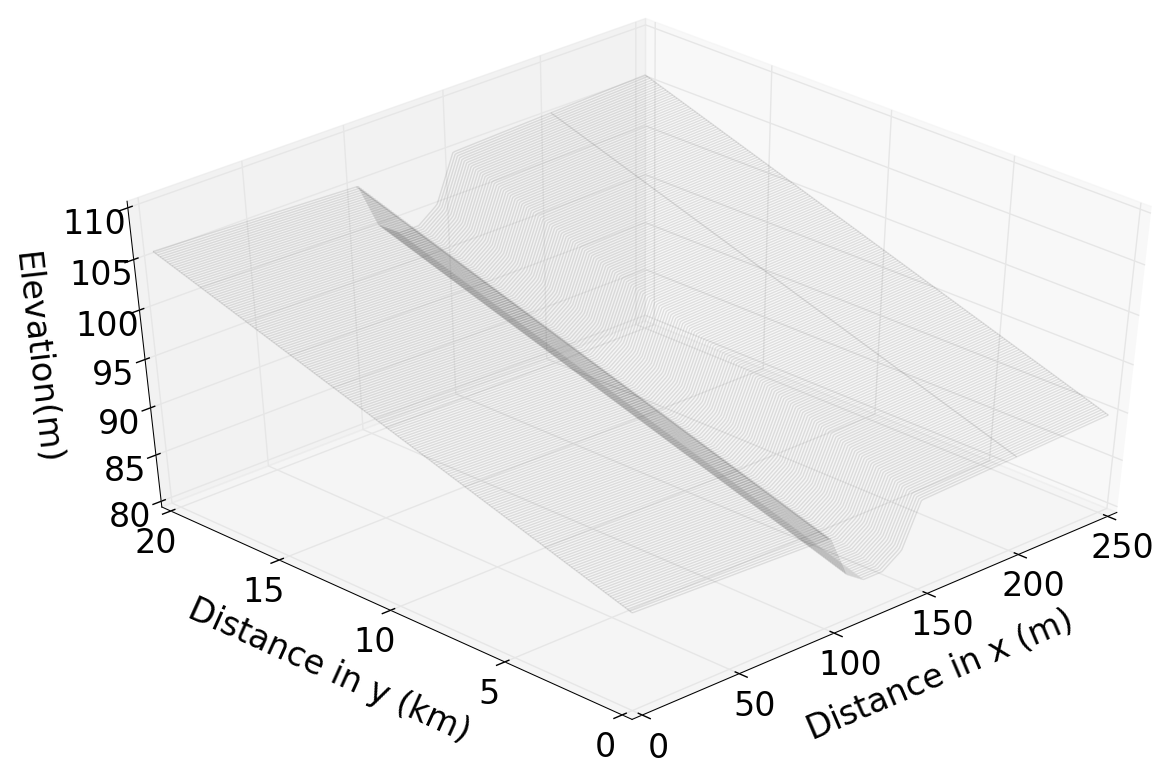
The test domain used in the experiments in this paper is the same as that used in Cooper et al. (2018) and is shown in Fig. 1. The domain has dimensions of 20 km by 250 m and describes a gently sloping valley and river channel (with an upstream–downstream slope of 0.08 %). The domain is split into grid cells of size 10 m by 10 m for computation. The river channel is prescribed to be the central five grid cells in the x direction for all values of y and is 50 m wide; the floodplain is defined as the rest of the domain. The slope of the floodplain towards the river is 0.8 % based on values derived from a DTM of a stretch of the river Severn in the U.K.
4.3 Twin experiments
We have carried out a number of twin experiments in order to illustrate and compare how well forecasts can be corrected when using the three different observation operator approaches. The experiments use a “truth” flood simulation and a forecast ensemble of flood realisations comprising 100 members. The forecast ensemble is updated using synthetic observations at several times during the simulation time; synthetic observations are created from the truth as described in Sect. 4.4. The analysis water levels (and parameter values) can then be compared to the true water levels (and parameter values) to see how well the assimilation corrects the forecast.
In this work, the truth flood is driven by a time-varying inflow based on data taken from a gauge on the river Severn during a flood in November–December 2012. The true inflow is shown in Fig. 2; the figure also shows the inflows driving the ensemble members. All the inflows used here were also used in the experiments reported in Cooper et al. (2018). Inflows for each ensemble member were generated by perturbing the true inflow with additive, time-correlated random errors. Time-correlated errors were generated for each ensemble inflow using a first-order autoregression (AR(1)) technique (Wilks, 2011) with a zero mean, according to
where ei,k is the error added to the inflow at the kth time step in the ith ensemble member. The term wi,k is taken from a normal distribution true inflow); i refers to ensemble member and k refers to the time step. The autocorrelation coefficient, r<1, was set to 0.997; this very high coefficient means that the errors are close to persistent in time for each ensemble member and that each inflow ensemble member is smooth. The standard deviation of the random part of the error corresponds to the value used to generate inflow errors in Garcia-Pintado et al. (2015) and results in inflows that fit within the range given in Di Baldassarre and Montanari (2009) (4 % to 43 %). The mean of the inflow ensemble has negligible bias relative to the true inflow. The experiments shown here all use the same inflow for the truth and the same set of perturbed inflows for the forecast ensemble. For a different true inflow and different ensemble inflow error realisations, the results obtained using the different observation operators may compare slightly differently. However, the mechanisms we describe would be the same.
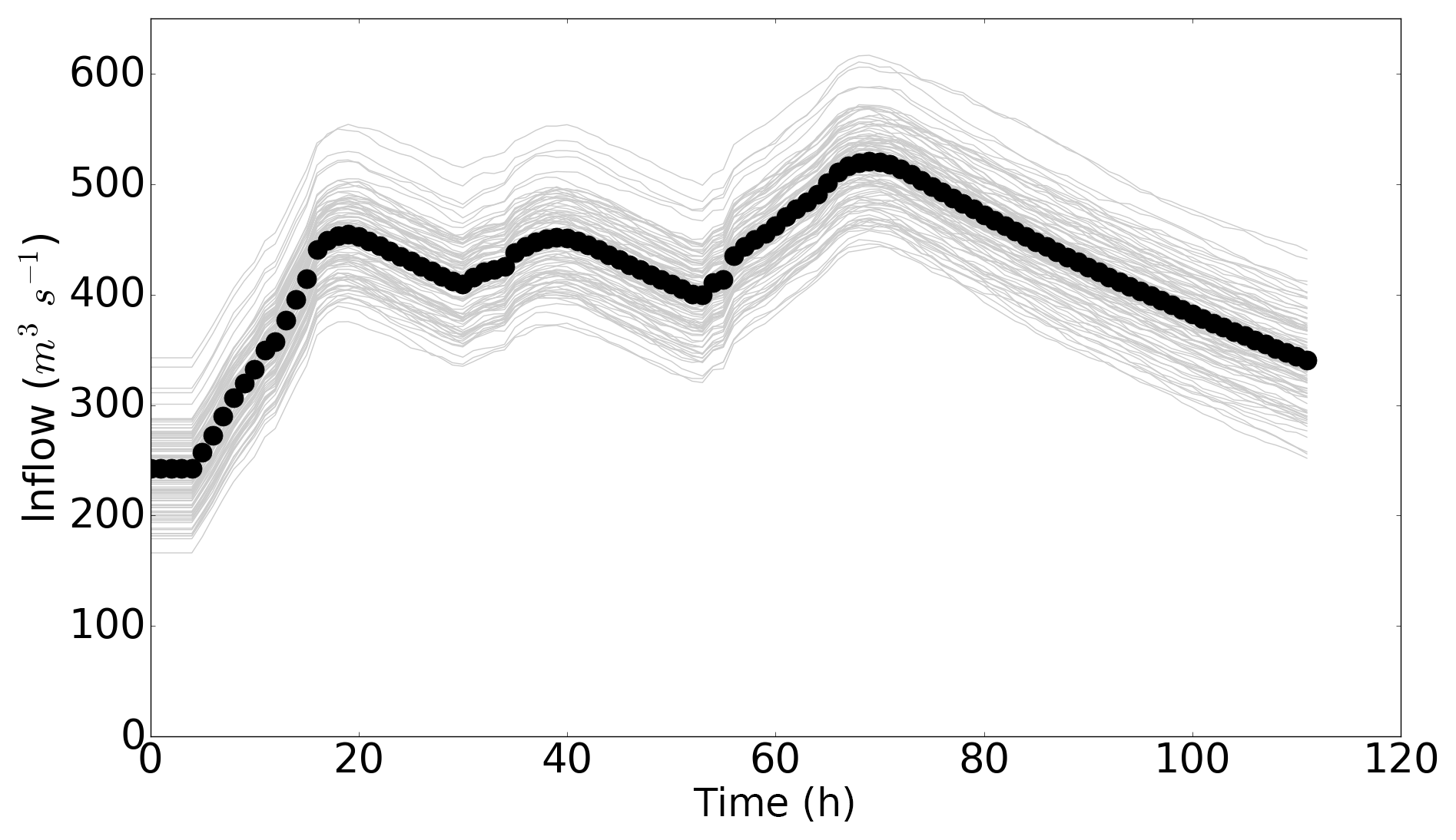
Figure 2Inflows with time. True inflow values are represented with circles, and ensemble inflows are shown by grey lines.
Each ensemble member was run with a different value of the channel friction parameter, nch. The behaviour of floodwater is highly sensitive to nch (Hostache et al., 2010; James et al., 2016), with low channel friction parameter values leading to water travelling through and leaving the domain more quickly. This leads to shallower water levels (and less flooding) in our simple domain for a given inflow. Conversely, higher channel friction parameter values lead to water moving slowly through the domain, leading to deeper water levels in the channel and more flooding. We chose a true value of nch=0.04, equal to the value for a natural stream given in Maidment and Mays (1988). For the initial forecast step, a value of nch for each forecast ensemble member was drawn from a normal distribution with the mean, μ, that is different to the true value and standard deviation σ. This imposed bias in the forecast ensemble channel friction parameter means that we can test how well data assimilation with different observation operators can correct the forecast state and parameter value towards the truth. In our state estimation experiments, the value of nch assigned to each ensemble member remained constant throughout the simulation. For joint state–parameter experiments, the values of nch were updated at each assimilation time through the ETKF equations, as described in Sect. 2.2. Using an incorrectly specified channel friction parameter in the forecast is realistic, as the true value is unlikely to be known in operational situations. Initial forecast channel friction parameters are randomly drawn from a normal distribution with μ=0.05 and σ=0.01 for experiments with positive bias in nch and with μ=0.03 and σ=0.01 for experiments with negative bias in nch. The true value of nch falls within 1 standard deviation of the mean of each initial nch distribution, and our choices of friction parameter values fit with the range used in Horritt and Bates (2002). On the floodplain the value of the friction parameter is likely to be higher than nch due to the effects of vegetation. In this paper we used a true value for the floodplain friction parameter of nfp=0.05; the same true value for nfp was used for each ensemble member. The value of this parameter is likely to have an impact on the dynamics of a flood event, but flooding is commonly understood to be less sensitive to nfp than nch (e.g. Hostache et al., 2010). Here we focus on the ability of the observation operators to update nch only.
4.4 Synthetic observations
In identical twin experiments, observations are generated from a truth run; in this case the truth flood simulation is described in Sect. 4.3. For the two conventional observation operators we selected six synthetic observations of water elevation at the true flood edge at y=500, 700, 900, 1100, 1300 and 1500 m. The elevation at these points is directly available from the state vector of water levels provided by our truth run. Each synthetic observation mimics an SAR-derived water level observation at a given cross section by locating a flood edge and using the true, calculated water elevation at this position as the observation. Here we define the flood-edge WLO to be the elevation at the first “dry” model cell encountered when moving in a perpendicular direction from the centre of the channel along one of our defined cross sections. (We use observations on the left-hand side of the domain, i.e. where x<125 m, but since the domain and inflows are symmetrical in our simple experiments, this choice is arbitrary; we could have instead used observations from the right-hand side of the channel or a combination of the two.) We added unbiased, Gaussian noise with a standard deviation of 0.25 mm to each observation; this is the same as the observation error used by Garcia-Pintado et al. (2015) in a case study. Observation error may be due to SAR instrument error or errors in determination of flood extent. The spacing of 200 mm between observations represents an optimistic best-case situation and is the same as the smallest recommended distance between thinned flood-edge values for use in an assimilation system in Mason et al. (2012) (note that the other selection criteria used in the paper are not applicable here due to the use of synthetic observations). In fact, more recent work suggests a much longer correlation length scale between observation errors in a real case study (Waller et al., 2018), in which the authors point out that part of the observation error correlation is due to the observation operator.
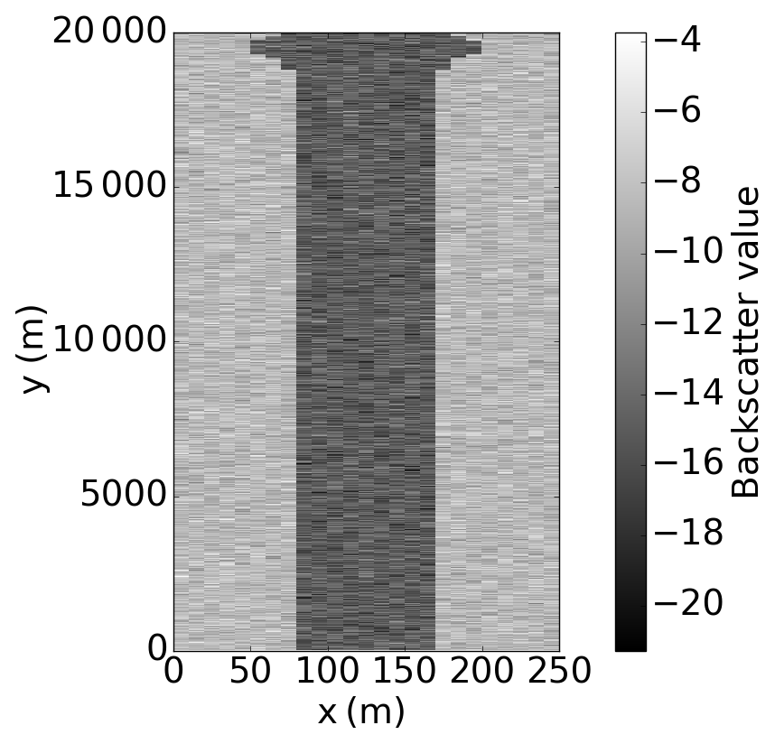
In order to test our backscatter observation operator, we require synthetic backscatter observations; we therefore create a synthetic SAR image from our truth run, comprising backscatter values in each cell. We can then extract synthetic backscatter observations at desired locations. We have taken a very simple approach to generating a simplified synthetic SAR image in order to perform proof-of-concept experiments with our new observation operator; we will apply the method to a real case study and real SAR images at a later date. To generate a synthetic SAR image, we have taken our truth run water level output and applied a threshold water level of 5 cm in each cell to determine which cells are wet and which are dry. Water levels below a threshold of a few centimetres are likely to be misclassified as dry in a real SAR image due to vegetation. Synthetic backscatter values are then assigned to each cell: dry cells are assigned a backscatter value drawn from , and wet cells are assigned a value from . For this, we have used values of , and σd=1.53, which are experimentally derived from an SAR image in Giustarini et al. (2016). An example simplified synthetic SAR image, generated from the truth run at t=40 h, is shown in Fig. 3.
In order to derive synthetic observations from the synthetic SAR image, the observation process is then carried out, i.e. we do the following:
-
We bin all the synthetic backscatter values in a histogram (see Fig. 4).
-
We fit two Gaussian curves to the synthetic backscatter values (using Python fitting algorithm scipy.optimize.curve_fit; see Fig. 4).
-
We extract new values of mw1, σw1, md1 and σd1 from these distributions; these values are naturally very similar to the experimental values used to create the synthetic SAR image. We use a different realisation of observation error for each synthetic image (i.e. at each observation time); typical values of mw1, σw1, md1 and σd1 are within 1 % of mw, σw, md and σd.
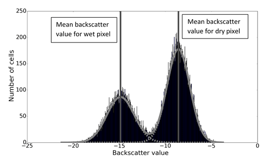
Figure 4Histograms and fitted Gaussian distributions of synthetic backscatter values. Dashed grey lines show two fitted Gaussian distributions, and the solid grey line shows the sum of the two fitted distributions. Vertical lines show the positions of the mean wet and dry backscatter values.
We then extract backscatter values to be synthetic observations. Although it would be possible to use a large number of backscatter observations in this method, for the experiments presented here we have not used all of the available synthetic observations. There are a number of reasons for limiting the number of observations. Firstly, observation errors are likely to be correlated for observations that come from positions close to each other in physical space. Some thinning of the observations is therefore necessary to meet the requirement that the observations used in the assimilation have uncorrelated errors (Mason et al., 2012); this allows use of a diagonal observation error covariance matrix. Secondly, without ensemble localisation, using a number of observations larger than the number of ensemble members can cause the assimilation algorithm to overfit the observations (Kepert, 2004).
In this study we wish to investigate the differences in the updates generated by different observation operator approaches. We therefore use equivalent observation information for each of the operators. In the case of the water level observation operators, we have used flood-edge water level observations at six locations, where the flood-edge location is defined as the position of the first dry model cell (see Sect. 4.4). For the new operator we use two backscatter observations for each transect.
Figure 5 shows a schematic of the locations of the observations we have used in this study, relative to the edge of the flood. All observations used in this study come from transects at y=500, 700, 900, 1100, 1300 and 1500 m. In practical application of the backscatter operator, observations could be used from any location covered by the SAR image.

Figure 5Schematic of observation locations used in this study for each transect in cross section. The black thick line shows the discretised domain elevation, and the blue dashed line shows the observed floodwater level. The arrows and green crosses show locations of the observations as labelled.
4.5 Observation error covariance matrices
It is important to specify the observation error statistics in data assimilation. In all cases we assume that our observation errors are uncorrelated so that we can use a diagonal error covariance matrix, R. We assume that the error in flood-edge WLOs is 0.25 m. This is close to the calculated error in SAR-derived water level observations in Mason et al. (2012) and is the same value used in Cooper et al. (2018) and Garcia-Pintado et al. (2015).
The uncertainty in each backscatter observation reflects the distribution to which it belongs (wet or dry). We assume that each entry can be set to be , corresponding to a dry observation, or for a wet observation.
4.6 Further experimental details
We present here the results from a number of data assimilation experiments, each lasting for a total simulation time of 112 h. This includes an initial spin-up period with constant inflow for 4 h (as shown in Fig. 2) to allow the water to reach an equilibrium state. In each experiment we use 100 forecast ensemble members. Assimilations are carried out at 12 h intervals. This is currently the shortest likely time between observations due to return times for satellites equipped with SAR instruments. The ETKF is used without localisation or inflation in all of the experiments, as we did not encounter any spurious correlations or problematic ensemble collapse (see Petrie and Dance, 2010). This suggests that the number of ensemble members, 100, is sufficient in this particular case.
Experiments were run as follows:
-
State-only estimation. State estimation experiments show how well data assimilation is able to correct forecast water levels at each observation time using the three different observation operators. In all of the experiments, a large bias is present in the forecast channel friction parameter values, which means that by design the error between the ensemble forecast and the truth grows quickly during each forecast step; the forecast corresponding to each of the observation operators relaxes to the same no-assimilation (open-loop) forecast. This allows us to examine the effect of each observation operator on the water levels in isolation at each observation and assimilation time, as the operators are each acting on very similar pre-assimilation forecasts.
State-only estimation experiments were carried out using a positive bias in the forecast channel friction parameter, which leads to forecast water levels that tend to be deeper than the truth (PBSO – positive bias in nch, state-only estimation – experiment) at any given cross section, and with a negative bias in the channel friction parameter, leading to shallower forecast water levels (NBSO – negative bias in nch, state-only estimation – experiment).
-
Joint state and parameter estimation. Updating the value of nch along with water levels allows us to see the effect of the observation operators on the forecast when the large parameter bias can also be corrected by the assimilation process. Correcting the channel friction parameter in this way leads to better persistence in the forecast correction (Cooper et al., 2018). Experiments were again carried out using both a positively biased initial channel friction parameter distribution for the forecast ensemble (PBJ – positive bias in nch, joint state–parameter estimation – experiment) and negatively biased initial channel friction parameter distribution (NBJ – negative bias in nch, joint state–parameter estimation – experiment).
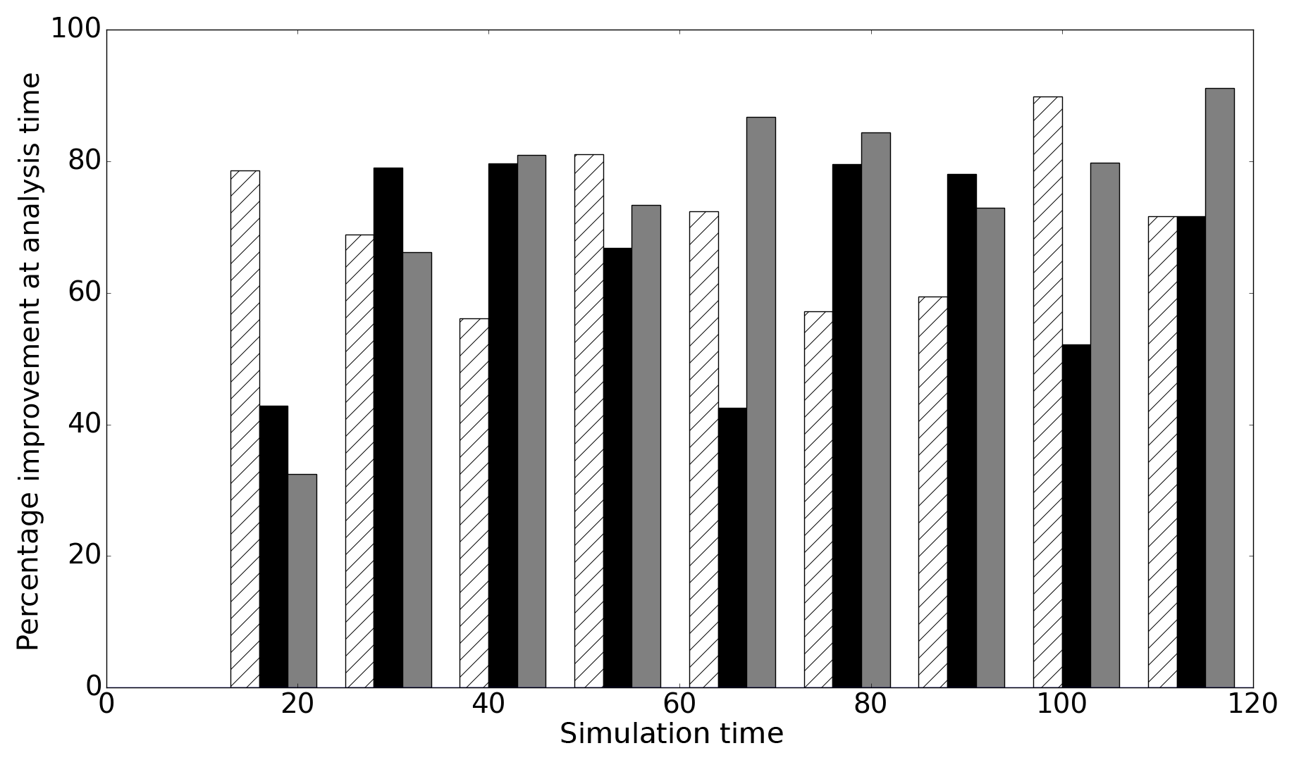
Figure 6Improvement in the forecast at each assimilation time (PBSO experiment). The hatched white bars show improvement for the hs operator, the black bars show improvement for the hnp observation operator and the grey bars show the improvement for the hb observation operator.
5.1 State-only estimation
5.1.1 Positive bias in forecast ensemble channel friction parameter (PBSO)
Figure 6 shows improvement in the analysis compared to the forecast at each observation time for the PBSO experiment. Improvement is defined as
where xt is the true state of the system. This improvement measure is positive when the error in the analysis is smaller than the error in the forecast, while negative values imply a larger error in the analysis than the forecast. A perfect analysis (xa=xt) would result in a 100 % improvement measure. Figure 6 shows that in the PBSO experiment all of the operators reduce the difference between the forecast mean and the truth at each observation time. We found that the error in the forecast then quickly relaxed back to the no-assimilation (open-loop) case for all of the observation operators. This short-lived persistence in forecast improvement (less than approximately 3 h here) when only water levels are updated is typical for such systems and is reported in many studies, including Cooper et al. (2018), Andreadis et al. (2007), Neal et al. (2009), Garcia-Pintado et al. (2013) and Matgen et al. (2010).
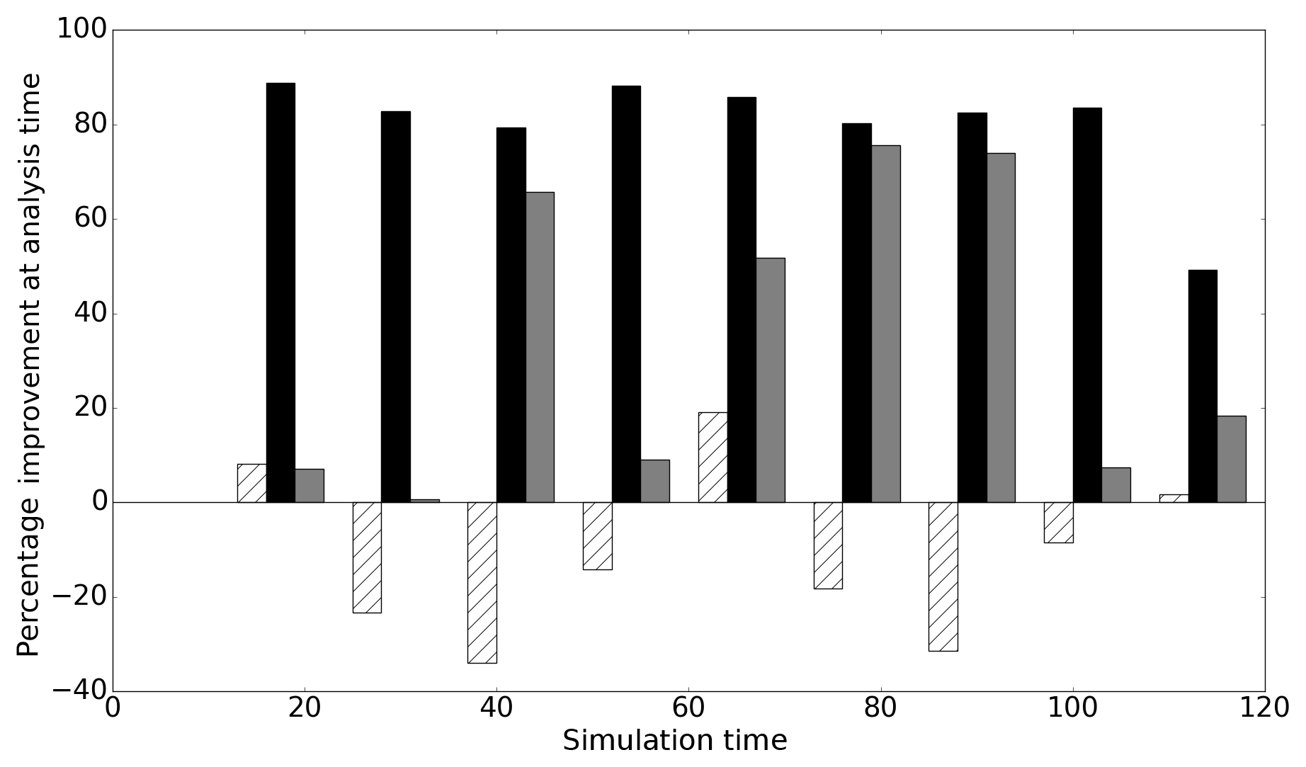
Figure 7Improvement in the forecast at each assimilation time (NBSO experiment). The white hatched bars show improvement for the hs operator, the black bars show improvement for the hnp observation operator and the grey bars show improvement for the hb observation operator.
5.1.2 Negative bias in forecast ensemble channel friction parameter (NBSO)
Figure 7 shows the improvement in the forecast at each assimilation time for the NBSO experiment. Here, the ensemble channel friction parameters are such that the mean forecast water level tends to be shallower than the truth at any given cross section in our domain. Unlike in the PBSO experiment, the operators do not all provide a good analysis at every observation time. In fact, assimilation of flood-edge observations using the simple flood-edge observation operator, hs, makes the forecast significantly worse at many assimilation times. The reason for this is illustrated by considering the innovation produced by the simple flood-edge operator when the forecast is shallower than the truth. The types of innovations produced for mean forecasts that are either deeper or shallower than the truth are shown in a schematic in Fig. 8.
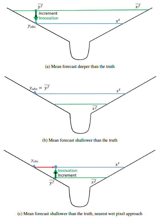
Figure 8Schematic showing innovation for flood-edge observation. In all cases blue lines represent the true water level, and blue circles represent the corresponding flood-edge observation, yobs. Green lines show the mean forecast water level, and green circles show the corresponding mean forecast–observation equivalent, . Innovations (δ) are shown with green arrows and increments by thinner black arrows; see Eq. (11) for definitions. The red arrow shows the difference between the observation location and the nearest wet pixel location.
Figure 8a shows a simple domain in a cross section where the mean forecast is deeper than the truth, with the innovation generated by the simple flood-edge operator. The innovation is such that the data assimilation algorithm can generate an increment and adjust the forecast water levels to be closer to the true water levels. However, as shown in Fig. 8b, when the mean forecast is shallower than the truth, the simple flood-edge assimilation method generates an innovation equal to zero. This is because the observation implies that at the flood edge, the water depth relative to the topography is zero; the ensemble forecast mean also predicts that the water depth is zero at the observation position. The increment is therefore also zero and the forecast cannot be adjusted to be closer to the truth (i.e. to shallower water levels), even though the observation clearly indicates that this is necessary. Figure 8c illustrates the way that the nearest wet pixel approach solves this problem by taking the water elevation at the observation position and extrapolating it in space. This effectively moves the observation location to the nearest wet pixel, allowing a non-zero innovation to be calculated.
Figure 8 illustrates the fact that the simple flood-edge operator cannot produce a useful update when the mean of the forecast ensemble is shallower than the observed water level. Figure 7 shows that in our experiments the simple flood operator in fact makes the forecast worse, increasing error relative to the truth at several assimilation times. The reason for this is linked to the fact that it is possible for the mean of the forecast ensemble to be deeper than the truth on the floodplain but shallower than the truth in the river channel.
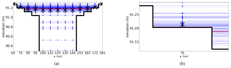
Figure 9Cross section of the domain showing bathymetry as a black solid line. The true water level is shown as a red dotted line, and water levels predicted by each ensemble member are shown as blue circles. The mean forecast in each model cell is shown as a cross. (a) shows the central part of the domain from m. (b) shows the forecast water levels and resulting forecast mean in the cell centred at 75 m in greater detail. Reprinted from Cooper et al. (2018), with permission from Elsevier.
Figure 9 shows the domain at one cross section. In Fig. 9 we see that in the channel (e.g. at x=125 m) the true water level is deeper than the ensemble mean. At the edge of the flood, the true water depth is (by definition) zero relative to the topography, and the majority of ensemble members also predict zero water depth in these cells. However, there are a small number of ensemble members that predict non-zero water depth at the flood edge; it follows that the ensemble mean at this location is therefore a small non-zero water depth as per Eq. (1). The flood-edge operator therefore generates an innovation such that the mean forecast water depth at the flood edge is reduced and the analysed water depths are closer to the truth at this location. Correlations between water levels in the domain mean that the water depth in the channel is also reduced by the update step; this increases the error relative to the truth in the channel. This explains the overall increase in error at assimilation times seen in Fig. 7.
The results in Figs. 6 and 7 show that the new backscatter operator works well at most of the observation times. The mechanism by which the backscatter observation operator works is illustrated in Fig. 10.
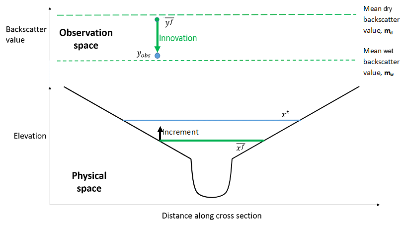
Figure 10Schematic of innovation in observation (backscatter) space and increment in physical space for one backscatter observation. The horizontal blue line represents the true water level, and the blue circle represents a corresponding backscatter observation, yobs. The solid green line shows the mean forecast water level, and the green circle shows the corresponding mean forecast–observation equivalent in observation space, . The innovation (defined in Eq. 11) is shown in observation space with a green arrow, and the increment in physical space at the observation position (Eq. 12) is represented by a thinner black arrow.
Figure 10 shows a simplified river channel in a cross section. The lower part of the figure shows an example of a true and mean forecast water level, as in Fig. 8. The upper part of the figure shows the same cross section but is a representation in observation space of an example (single) observation and equivalent mean forecast backscatter value, . The green circle in observation space shows in the cell at the observation position. The value of is calculated using water levels forecast by all the ensemble members, through Eq. (21), and is essentially a measure of the proportion of ensemble members which predict that cell to be wet (or dry). The mean forecast backscatter, , will always take a value between the mean observed wet value, mw1, and the mean observed dry value, md1; if half the ensemble members predict a cell to be dry and half predict it to be wet, the value of will lie halfway between mw1 and md1. If most ensemble members predict the cell to be wet (dry), the value of will be close to the mean observed wet (dry) backscatter value. The observed backscatter value, yobs, is shown as a blue circle in observation space.
The innovation is shown in observation space in Fig. 10. The innovation is the difference between the observed backscatter value, yobs, and the mean forecast backscatter value, . Figure 10 shows that for the hs and hnp the state variables and observed variables are the same. In the approach using hb, the observations are different to the state variables. For hb the increment is the calculated difference in the water level between the forecast and the analysis in metres, but this is calculated using an innovation that is a difference in the backscatter value between the model and the observation. In the example shown, the mean forecast backscatter value indicates that most of the ensemble members predict the cell containing the observation position to be dry. This corresponds to the shallow mean water level prediction shown in physical space. The backscatter observation indicates that the cell is wet. The innovation is therefore large and indicates that the cell is more likely to be wet than the forecast indicates. This maps into an increment in physical space through Eq. (12) such that the calculated analysis water level at the observation position is deeper than the forecast water level.
A potential problem with the backscatter operator can be illustrated through inspection of Eqs. (13) and (10). Equation (10) shows that when the value of the Kalman gain matrix is zero, there can be no update to the forecast through assimilation of observations, even when there is a large innovation – i.e. a large difference between a model prediction and an observation. Equation (13) shows that this K=0 condition can be met if either X=0 or Y=0. For Y=0 to be true, it is only required that the ensemble members all predict the cell containing the observation to be dry or that all ensemble members predict the cell to be wet. This is because if all ensemble members predict a cell to be wet, then they all give the same value of through Eq. (22). Equation (21) then shows that the value of will then also be equal to mw, and each term in Y must therefore be zero according to Eq. (9), since all the ensemble members are the same as the mean. This means that if all the ensemble members predict different but positive water depths (i.e. no non-zero water depths are predicted in the ensemble), no increment can be generated and no update can be made to the forecast, regardless of whether the observation indicates a wet or dry condition. For this reason, observations at or near the edge of the flood are most valuable to the data assimilation algorithm when using the backscatter observation operator, since these are locations where it is most likely that the ensemble members will predict a variety of wet–dry predictions. We did not observe any situation in which Y=0 in these experiments. It would in principle be possible to add a small amount of noise to each value of in order to prevent Y=0, but this risks generating an innovation and increment such that the analysis error is larger than the forecast error.
5.2 Joint state–parameter estimation
The large source of error in these experiments is, by design, due to a large bias in the forecast ensemble channel friction parameter values. In this section we show the results of updating the forecast channel friction parameter values as part of the assimilation process. One way to measure the effectiveness of a data assimilation approach is to compute the root-mean-square error (RMSE) between the resulting forecast and the truth. Here, the RMSE is defined as
where is true water depth in the jth cell; is mean forecast water depth in the same cell. As before, N represents the number of cells in the domain.
5.2.1 Positive bias in forecast ensemble channel friction parameter (PBJ)
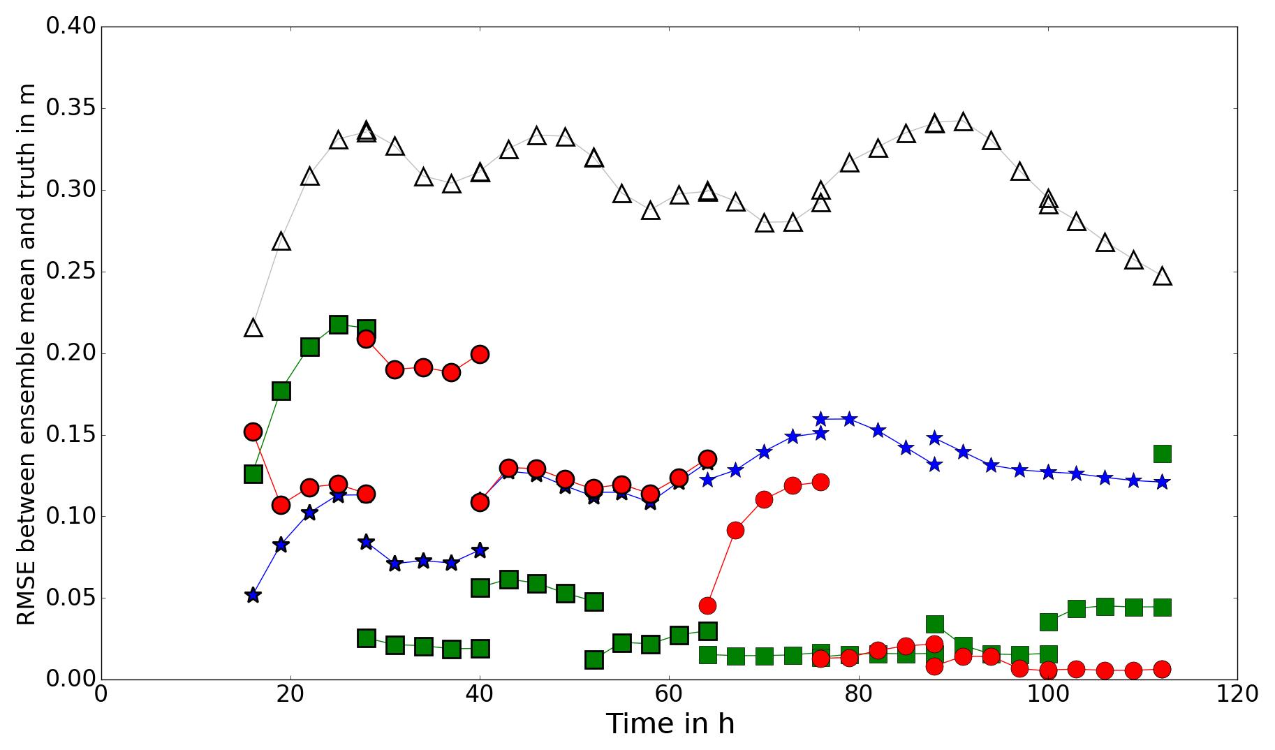
Figure 11RMSE between forecast and truth (PBJ experiment). Open triangles show the RMSE between the open-loop forecast and the truth. Blue stars, green squares and red circles show the RMSE between the forecast mean and the truth, using the hs, hnp and hb observation operators respectively.
Figure 11 shows the RMSE between the mean water levels predicted by the model and the true water levels for the PBJ experiment. The mean value of nch and the mean value of the predicted water levels are updated at 12 h intervals starting from 16 h. At each assimilation time the RMSE for both the forecast (pre-assimilation) and analysis (post-assimilation) water levels are shown; points within a forecast step are joined with a line. The results show that the assimilation leads to a much improved forecast of water levels for all of the operators at all times. There is persistence in the improvement to the forecast, and each of the observation operators provides a better forecast than the open-loop ensemble for the whole of the simulation time. The results obtained using the hs operator converge to higher RMSE values than the other two operators. Use of the hb operator shows a gradual reduction in RMSE over successive forecast–analysis cycles. The results for the hnp operator show faster reduction in the RMSE values, but the final analysis value (at 112 h) has a much higher RMSE. This is because at 112 h the inflow has reduced such that the water is well back within the bank, and in these conditions the assumptions used to derive water elevation observations break down; the sides of the river are too steep for the water edge position to accurately determine elevation. In an operational setting, it would be necessary to test for an in-bank condition and discard observations for the hnp operator when the river is within the bank. This means that it is not possible to calibrate a hydrodynamic model on a river using SAR images when it is not flooding if water level observations are being used (i.e. with either the hs or hnp observation operator).

Figure 12Calculated analysis mean channel friction parameter (PBJ experiment). Red horizontal line shows true value of channel friction parameter. Error bars show one standard deviation of ensemble parameter distribution.
Figure 12 shows the calculated (analysis) mean channel friction parameter values at each assimilation time for the three observation operators. All of the operators produce values for the parameter that are closer to the truth than the initial value. The value of the channel friction parameter calculated using the hb observation operator converges to a value close to the truth after six observations and then remains there. The value calculated using hnp converges more quickly to a value close to the truth, but the last value in the time series (at 112 h) then diverges from the true value. This is because the river is now well within the bank and water elevation observations cannot be reliably determined.
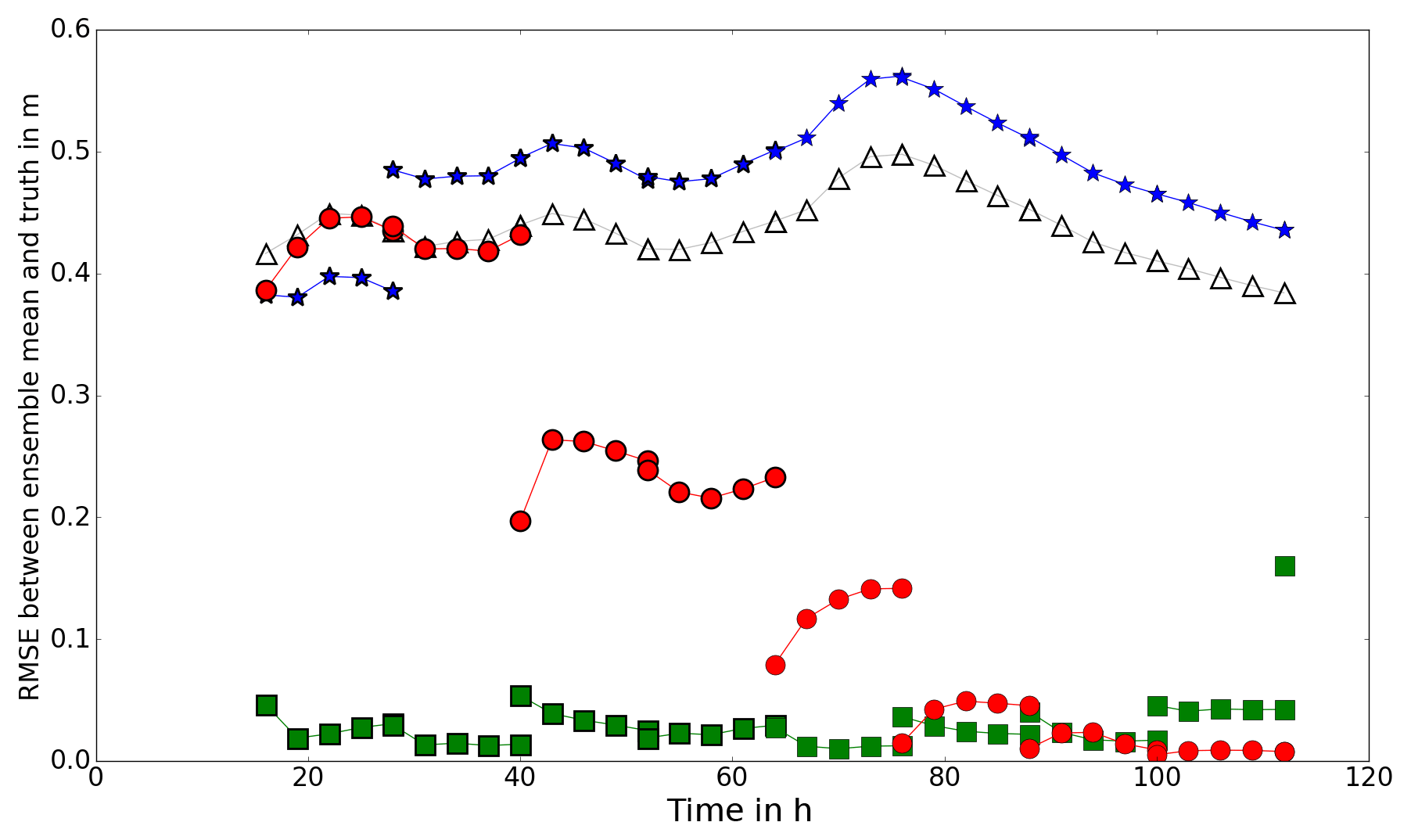
Figure 13RMSE between forecast and truth (NBJ experiment). Open triangles show the RMSE between the open-loop forecast and the truth. Blue stars, green squares and red circles show the RMSE between the forecast mean and the truth, using the hs, hnp and hb observation operators respectively.
5.2.2 Negative bias in forecast ensemble channel friction parameter (NBJ)
Figure 13 shows the RMSE between the forecast and the truth for the NBJ experiment. The nearest wet pixel approach provides a forecast which is very close to the truth for most of the simulation time. The backscatter operator performs well after the first two assimilation steps, showing a slower convergence to the true solution as in the PBJ experiments. The simple flood-edge operator performs badly, leading to a forecast which is worse than the open-loop case for most of the time. The reason for the poor performance in this particular experiment is likely due to the mechanisms outlined in Sect. 5.1.2. The forecast is adjusted in the wrong direction at the first assimilation time (at 16 h) such that the water levels are too shallow; the mechanism by which this can happen is demonstrated in Fig. 9. All subsequent corrections are very close to zero, due to the mechanisms illustrated in Fig. 8, so that the blue line appears to be unbroken.
Figure 14Calculated analysis mean channel friction parameter (NBJ experiment). Horizontal red line shows true value of channel friction parameter. Error bars show one standard deviation of ensemble parameter distribution.
Figure 14 shows the calculated analysis mean channel friction parameter values at each assimilation time in the NBJ experiment for the three observation operators. The results for the simple flood-edge operator support the scenario outlined above, whereby the friction parameter is initially adjusted in the wrong direction and then cannot be updated towards the truth. Although the details of this will depend on topography, observation error, and choice of forecast inflows and parameters, this is nevertheless an important mechanism to consider when choosing an observation operator. Both the hnp and hb operators do successfully correct the value of the parameter towards the truth, with the hnp operator recovering a good value in a shorter time than the hb operator. Both Figs. 13 and 14 show that at the final assimilation time, the analysis and parameter value provided by the nearest wet pixel operator are not close to the truth. Again, this is because the river is well within the bank, so the flood-edge observation is on ground which is too steep to provide a good observation; in operational settings observations such as these would be screened out and no update would be made with the operator.
In this study we have chosen to use a small number of backscatter observations for our experiments. This allowed us to compare updates between the three observation operators when the observation operators were all given equivalent information; in this way we can draw conclusions about the physical mechanisms responsible for the different updates. In a real case, one of the major advantages of using our new backscatter observation operator is that it would be possible to use a large number of backscatter observations compared to the number of water level observations which are typically available. The availability of a large number of observations may be a major strength of our new approach; in our simple experiments (not shown) we found that assimilating a larger number of observations with the backscatter operator provided a better analysis than using only a few. Another merit of the backscatter operator is that there is less processing involved in using backscatter observations directly, potentially reducing the amount of time between acquisition of an SAR image and its use to update an inundation forecast. The backscatter operator also removes the need for locating the nearest wet pixel in the model forecast, which can be computationally costly.
There are a number of potential problems with practical implementation of the backscatter operator. One is that using histograms to produce SAR-derived inundation maps can lead to errors in assigning pixels to wet–dry categories. One way to deal with this would be to use region-growing techniques (see e.g. Horritt et al., 2001) or change-detection techniques (see e.g. Hostache et al., 2012) to produce robust wet–dry maps for SAR images and then perform a quality control procedure to discard any backscatter observations which would lead to misclassification due to, for example, emergent vegetation. This procedure would remove the advantage of fewer processing steps for the backscatter operator but may not be necessary. Further research is required to understand how robust the method is to the proportion of misclassified SAR pixels in a real case study. We note that the backscatter operator would not generate an update the forecast in model cells that all the ensemble members predicted to be dry (or wet) as discussed in the last paragraph of Sect. 5.1.2. This means that SAR pixels far from the river wrongly classified as wet or SAR pixels in the river channel wrongly classified as dry would not degrade the forecast through an erroneous update.
The new backscatter operator is likely to work well in cases where good separation of the wet–dry distributions can be obtained through a histogram and works less well in cases where the distributions overlap. The new observation operator does not require a digital elevation model to generate forecast–observation equivalents, although the hydrodynamic model would require topography information to generate a forecast. Water level observations cannot be accurately determined in areas with high slope, whereas backscatter observations will be unaffected. Like the other observation operators, the new operator will likely provide better results in rural settings than urban settings; double-bounce and layover effects due to buildings are potential sources of problems for all of the operators (Mason et al., 2018).
We have carried out a series of experiments to test the performance of three different types of observation operators in an ETKF approach to data assimilation for fluvial inundation forecasting. Although the results are for one specific idealised domain, one realisation of true inflow and a single realisation of observation error per observation type, we believe that many of our conclusions will be applicable much more widely through the mechanisms we describe. Repeats of experiments (not reported here) with different realisations of observation error show evidence of the same behaviour in terms of the mechanisms we have described. Our experiments show the following:
-
Simple assimilation of flood-edge water elevation observations can result in no correction to the forecast even when there is a large difference between the forecast and the observation. This happens when both the model prediction and the observation predict no flooding at the observation location. We have illustrated the physical mechanism responsible for this (Fig. 8) and shown an example in which this happens in our experiments (see assimilation times from 28 h onwards in Fig. 13). The simple flood-edge operator can also generate an update such that the analysis has a larger error than the forecast. This can occur when the forecast is deeper than the truth at the observation position but shallower than the truth in the channel. In such cases the assimilation updates the water levels to shallower levels as required at the observation position but also wrongly updates the channel water levels to be shallower. The mechanism for this is shown in Fig. 9; this is responsible for the negative improvement measures in the NBSO experiments (see Fig. 7). We have shown in our experiments that the simple flood-edge operator fails in these ways when the mean ensemble channel friction parameter is negatively biased, but it would also fail if, for example, the mean forecast inflow was negatively biased, since errors in friction parameter and inflow are correlated (Cooper et al., 2018). Since in operational settings both forecast inflow and channel friction parameter values are uncertain, we conclude that the simple flood-edge operator is not a good choice.
-
The nearest wet pixel approach provides better assimilation accuracy than simple flood-edge assimilation: in our experiments we find no evidence of negative “improvement” scores or zero increments when the forecast and observations are very different. In our idealised system it is the best choice of observation operator in terms of better forecast accuracy in the state-only experiments and in terms of rapid convergence to the true solution for both water levels and the mean channel friction parameter value in the joint state–parameter experiments. However, we have shown that using water edge observations when the river is well within bank can lead to a degradation of the forecast. Also, locating the nearest wet pixel is likely to be difficult in practice for operational applications using real, more complicated topography. One way to limit the distance between the flood-edge observation position and the nearest wet pixel is to locate the nearest pixel at which some threshold of ensemble members predict a positive water depth. The predicted water elevations at this location could then be used to create . This approach balances out the need to include information from ensemble members predicting shallow water levels at the observation position, with the requirement that the nearest wet pixel is not too far from the observation location.
-
Our new backscatter observation operator performs well compared to more conventional options in our idealised domain using synthetic observations. The operator does not suffer from the problems of the simple flood-edge operator and is able to correct the forecast for the state-only assimilation cases. The backscatter operator approach also allowed the forecast to converge to the true solution for both water levels and channel friction parameter value in the joint state–parameter experiments, although in our experiments convergence was slower than for the nearest wet pixel approach. Using backscatter values operationally may speed up the time taken from image acquisition to assimilation and an improved forecast due to fewer steps in the processing. The new operator could also potentially allow the use of much more information from any given SAR image, although there is likely to be a limit to the number of backscatter observations that can be used without causing variance collapse in the channel friction parameter distribution. Tests using larger numbers of backscatter observations have not been presented here; we plan to address this question in a real case study so that the results will be more directly applicable to real world situations.
This work has shown that our novel backscatter operator has the potential to improve inundation forecasting in fluvial floods, and we believe it may have applications in other types of flooding where SAR images are available. Further work is required to test the operator against the hnp approach in a real case study, using real SAR data and real topography in order to further assess the strengths and weaknesses of the different approaches. We have explained the physical mechanisms associated with the assimilation increments for each type of observation operator; these mechanisms will also be applicable to variational data assimilation methods using similar observations. Improved understanding of these physical mechanisms provides insight into the best approaches to improve the effectiveness of assimilation of SAR data in the future.
The inundation simulations in this work were generated using Clawpack 5.2.2, a collection of Fortran and Python code available from http://www.clawpack.org/ (copyright© 1994–2017, the Clawpack Development Team; all rights reserved; see website for licensing information). Details of the amended Clawpack source code as used in this work are freely available on request from the corresponding author, as is the Python code used to perform data assimilation on the inundation simulation output. Please contact e.s.cooper@pgr.reading.ac.uk for details.
ESC ran the experiments and drafted the paper. SD, JG-P, NN and PS contributed to analysis of the results, the discussion and manuscript editing.
The authors declare that they have no conflict of interest.
The authors gratefully acknowledge CASE sponsorship for ESC from the Satellite Applications Catapult and partial support for NKN from the NERC National Centre for Earth Observation (NCEO).
This research has been supported by the Natural Environment Research Council (grant nos. NE/L002566/1, NE/K00896X/1 and NE/K008900/1) and the Engineering and Physical Sciences Research Council (grant no. EP/P002331/1).
This paper was edited by Nunzio Romano and reviewed by two anonymous referees.
Andreadis, K. M., Clark, E. A., Lettenmaier, D. P., and Alsdorf, D. E.: Prospects for river discharge and depth estimation through assimilation of swath-altimetry into a raster-based hydrodynamics model, Geophys. Res. Lett., 34, L10403, https://doi.org/10.1029/2007GL029721, 2007. a
Baldassarre, G. D., Schumann, G., and Bates, P. D.: A technique for the calibration of hydraulic models using uncertain satellite observations of flood extent, J. Hydrol., 367, 276–282, https://doi.org/10.1016/j.jhydrol.2009.01.020, 2009. a
Barthélémy, S., Ricci, S., Le Pape, E., Rochoux, M., Thual, O., Goutal, N., Habert, J., Piacentini, A., Jonville, G., Zaoui, F., and Gouin, P.: Ensemble-based algorithm for error reduction in hydraulics in the context of flood forecasting, E3S Web of Conferences, 7, 18022, 2016. a
Bishop, C. H., Etherton, B. J., and Majumdar, S. J.: Adaptive Sampling with the Ensemble Transform Kalman Filter, Part I: Theoretical Aspects, Mon. Weather Rev., 129, 420–436, https://doi.org/10.1175/1520-0493(2001)129<0420:ASWTET>2.0.CO;2, 2001. a
Brown, K. M., Hambidge, C. H., and Brownett, J. M.: Progress in operational flood mapping using satellite synthetic aperture radar (SAR) and airborne light detection and ranging (LiDAR) data, Prog. Phys. Geog., 40, 196–214, https://doi.org/10.1177/0309133316633570, 2016. a, b, c
Chini, M., Hostache, R., Giustarini, L., and Matgen, P.: A Hierarchical Split-Based Approach for Parametric Thresholding of SAR Images: Flood Inundation as a Test Case, IEEE T. Geosci. Remote, 55, 6975–6988, https://doi.org/10.1109/TGRS.2017.2737664, 2017. a
Clawpack Development Team: Clawpack software, version 5.2.2., available at: http://www.clawpack.org (last access: 18 May 2019), 2014. a
Cooper, E., Dance, S., Garcia-Pintado, J., Nichols, N., and Smith, P.: Observation impact, domain length and parameter estimation in data assimilation for flood forecasting, Environ. Modell. Softw., 104, 199–214, https://doi.org/10.1016/j.envsoft.2018.03.013, 2018. a, b, c, d, e, f, g, h, i, j, k
Di Baldassarre, G. and Montanari, A.: Uncertainty in river discharge observations: a quantitative analysis, Hydrol. Earth Syst. Sci., 13, 913–921, https://doi.org/10.5194/hess-13-913-2009, 2009. a
Evensen, G., Dee, D. P., and Schröter, J.: Parameter Estimation in Dynamical Models, Springer Netherlands, Dordrecht, https://doi.org/10.1007/978-94-011-5096-5_16, 373–398, 1998. a
Garcia-Pintado, J., Neal, J. C., Mason, D. C., Dance, S. L., and Bates, P. D.: Scheduling satellite-based SAR acquisition for sequential assimilation of water level observations into flood modelling, J. Hydrol., 495, 252–266, https://doi.org/10.1016/j.jhydrol.2013.03.050, 2013. a, b, c, d, e, f
Garcia-Pintado, J., Mason, D., Dance, S. L., Cloke, H., Neal, J. C., Freer, J., and Bates, P. D.: Satellite-supported flood forecasting in river networks: a real case study, J. Hydrol., 523, 706–724, https://doi.org/10.1016/j.jhydrol.2015.01.084, 2015. a, b, c, d, e, f, g
George, D. L.: Augmented Riemann solvers for the shallow water equations over variable topography with steady states and inundation, J. Comput. Phys., 227, 3089–3113, 2008. a
Giustarini, L., Matgen, P., Hostache, R., Montanari, M., Plaza, D., Pauwels, V. R. N., De Lannoy, G. J. M., De Keyser, R., Pfister, L., Hoffmann, L., and Savenije, H. H. G.: Assimilating SAR-derived water level data into a hydraulic model: a case study, Hydrol. Earth Syst. Sci., 15, 2349–2365, https://doi.org/10.5194/hess-15-2349-2011, 2011. a, b
Giustarini, L., Hostache, R., Kavetski, D., Chini, M., Corato, G., Schlaffer, S., and Matgen, P.: Probabilistic Flood Mapping Using Synthetic Aperture Radar Data, IEEE T. Geosci. Remote, 54, 6958–6969, https://doi.org/10.1109/TGRS.2016.2592951, 2016. a, b, c, d, e
Golub, G. H. and Van Loan, C. F.: Matrix computations. 1996, Johns Hopkins University, Press, Baltimore, MD, USA, 374–426, 1996. a
Grimaldi, S., Li, Y., Pauwels, V. R. N., and Walker, J. P.: Remote Sensing-Derived Water Extent and Level to Constrain Hydraulic Flood Forecasting Models: Opportunities and Challenges, Surv. Geophys., 37, 977–1034, https://doi.org/10.1007/s10712-016-9378-y, 2016. a
Henry, J.-B., Chastanet, P., Fellah, K., and Desnos, Y.-L.: Envisat multi/-polarized ASAR data for flood mapping, Int. J. Remote Sens., 27, 1921–1929, https://doi.org/10.1080/01431160500486724, 2006. a
Horritt, M. and Bates, P.: Evaluation of 1-D and 2-D numerical models for predicting river flood inundation, J. Hydrol., 268, 87–99, https://doi.org/10.1016/S0022-1694(02)00121-X, 2002. a
Horritt, M. S., Mason, D. C., and Luckman, A. J.: Flood boundary delineation from Synthetic Aperture Radar imagery using a statistical active contour model, Int. J. Remote Sens., 22, 2489–2507, https://doi.org/10.1080/01431160116902, 2001. a, b
Hostache, R., Lai, X., Monnier, J., and Puech, C.: Assimilation of spatially distributed water levels into a shallow-water flood model, Part II: Use of a remote sensing image of Mosel River, J. Hydrol., 390, 257–268, https://doi.org/10.1016/j.jhydrol.2010.07.003, 2010. a, b
Hostache, R., Matgen, P., and Wagner, W.: Change detection approaches for flood extent mapping: How to select the most adequate reference image from online archives?, Int. J. Appl. Earth Obs., 19, 205–213, https://doi.org/10.1016/j.jag.2012.05.003, 2012. a, b
Hostache, R., Chini, M., Giustarini, L., Neal, J., Kavetski, D., Wood, M., Corato, G., Pelich, R.-M., and Matgen, P.: Near real-time assimilation of SAR derived flood maps for improving flood forecasts, Water Resour. Res., 54, 5516–5535, https://doi.org/10.1029/2017WR022205, 2018. a
James, T. S. S., Francesca, P., Paul, B., Jim, F., and Thorsten, W.: Quantifying the importance of spatial resolution and other factors through global sensitivity analysis of a flood inundation model, Water Resour. Res., 52, 9146–9163, https://doi.org/10.1002/2015WR018198, 2016. a
Kalman, R. E.: A New Approach to Linear Filtering and Prediction Problems, J. Basic Eng.-T. ASME, 82, 35–45, 1960. a
Kepert, J. D.: On ensemble representation of the observation-error covariance in the Ensemble Kalman Filter, Ocean Dynam., 54, 561–569, https://doi.org/10.1007/s10236-004-0104-9, 2004. a
Lai, X. and Monnier, J.: Assimilation of spatially distributed water levels into a shallow-water flood model, Part I: Mathematical method and test case, J. Hydrol., 377, 1–11, https://doi.org/10.1016/j.jhydrol.2009.07.058, 2009. a
LeVeque, R. J.: Finite Volume Methods for Hyperbolic Problems, Cambridge University Press, 2002. a
Livings, D.: Aspects of the Kalman filter, MSc thesis, Unversity of Reading, available at: http://www.reading.ac.uk/web/FILES/maths/Livings.pdf (last access: 18 May 2019), 2005. a
Livings, D. M., Dance, S. L., and Nichols, N. K.: Unbiased ensemble square root filters, Physica D, 237, 1021–1028, https://doi.org/10.1016/j.physd.2008.01.005, 2008. a, b
Maidment, D. and Mays, L.: Applied Hydrology, McGraw-Hill series in water resources and environmental engineering, Tata McGraw-Hill Education, p. 35, 1988. a
Mandli, K. T., Ahmadia, A. J., Berger, M., Calhoun, D., George, D. L., Hadjimichael, Y., Ketcheson, D. I., Lemoine, G. I., and LeVeque, R. J.: Clawpack: building an open source ecosystem for solving hyperbolic PDEs, PeerJ Computer Science, 2, e68, https://doi.org/10.7717/peerj-cs.68, 2016. a
Mason, D., Bates, P., and Amico, J. D.: Calibration of uncertain flood inundation models using remotely sensed water levels, J. Hydrol., 368, 224–236, https://doi.org/10.1016/j.jhydrol.2009.02.034, 2009. a, b
Mason, D., Schumann, G.-P., Neal, J., Garcia-Pintado, J., and Bates, P.: Automatic near real-time selection of flood water levels from high resolution Synthetic Aperture Radar images for assimilation into hydraulic models: A case study, Remote Sens. Environ., 124, 705–716, https://doi.org/10.1016/j.rse.2012.06.017, 2012. a, b, c, d, e
Mason, D. C., Dance, S. L., Vetra-Carvalho, S., and Cloke, H. L.: Robust algorithm for detecting floodwater in urban areas using synthetic aperture radar images, J. Appl. Remote Sens., 12, 045011, https://doi.org/10.1117/1.JRS.12.045011, 2018. a
Matgen, P., Schumann, G., Henry, J.-B., Hoffmann, L., and Pfister, L.: Integration of SAR-derived river inundation areas, high-precision topographic data and a river flow model toward near real-time flood management, Int. J. Appl. Earth Obs., 9, 247–263, https://doi.org/10.1016/j.jag.2006.03.003, 2007. a, b, c
Matgen, P., Montanari, M., Hostache, R., Pfister, L., Hoffmann, L., Plaza, D., Pauwels, V. R. N., De Lannoy, G. J. M., De Keyser, R., and Savenije, H. H. G.: Towards the sequential assimilation of SAR-derived water stages into hydraulic models using the Particle Filter: proof of concept, Hydrol. Earth Syst. Sci., 14, 1773–1785, https://doi.org/10.5194/hess-14-1773-2010, 2010. a, b
Matgen, P., Hostache, R., Schumann, G., Pfister, L., Hoffmann, L., and Savenije, H.: Towards an automated SAR-based flood monitoring system: Lessons learned from two case studies, Phys. Chem. Earth, 36, 241–252, https://doi.org/10.1016/j.pce.2010.12.009, 2011. a
Navon, I.: Practical and theoretical aspects of adjoint parameter estimation and identifiability in meteorology and oceanography, Dynam. Atmos. Oceans, 27, 55–79, https://doi.org/10.1016/S0377-0265(97)00032-8, 1998. a
Neal, J., Schumann, G., Bates, P., Buytaert, W., Matgen, P., and Pappenberger, F.: A data assimilation approach to discharge estimation from space, Hydrol. Proc., 23, 3641–3649, https://doi.org/10.1002/hyp.7518, 2009. a, b, c
Ott, E., Hunt, B. R., Szunyogh, I., Zimin, A. V., Kostelich, E. J., Corazza, M., Kalnay, E., Patil, D. J., and Yorke, J. A.: A local ensemble Kalman filter for atmospheric data assimilation, Tellus A, 56, 415–428, https://doi.org/10.3402/tellusa.v56i5.14462, 2004. a
Oubanas, H.: Variational assimilation of satellite data into a full saint-venant based hydraulic model in the context of ungauged basins, Theses, 1–202, 2018. a
Oubanas, H., Gejadze, I., Malaterre, P.-O., Durand, M., Wei, R., Frasson, R. P. M., and Domeneghetti, A.: Discharge Estimation in Ungauged Basins Through Variational Data Assimilation: The Potential of the SWOT Mission, Water Resour. Res., 54, 2405–2423, https://doi.org/10.1002/2017WR021735, 2018a. a
Oubanas, H., Gejadze, I., Malaterre, P.-O., and Mercier, F.: River discharge estimation from synthetic SWOT-type observations using variational data assimilation and the full Saint-Venant hydraulic model, J. Hydrol., 559, 638–647, https://doi.org/10.1016/j.jhydrol.2018.02.004, 2018b. a
Petrie, R. E. and Dance, S. L.: Ensemble-based data assimilation and the localisation problem, Weather, 65, 65–69, https://doi.org/10.1002/wea.505, 2010. a
Ricci, S., Piacentini, A., Thual, O., Le Pape, E., and Jonville, G.: Correction of upstream flow and hydraulic state with data assimilation in the context of flood forecasting, Hydrol. Earth Syst. Sci., 15, 3555–3575, https://doi.org/10.5194/hess-15-3555-2011, 2011. a
Rochoux, Mélanie, C.: Towards a more comprehensive monitoring of wildfire spread: Contributions of model evaluation and data assimilation strategies, Theses, Ecole Centrale Paris, available at: https://tel.archives-ouvertes.fr/tel-01130329 (last access: 18 May 2019), 2014. a
Rochoux, M., Collin, A., Zhang, C., Trouvé, A., Lucor, D., and Moireau, P.: Front shape similarity measure for shape-oriented sensitivity analysis and data assimilation for Eikonal equation, available at: https://hal.inria.fr/hal-01625575 (last access: 19 May 2019), ESAIM: Proceedings and Surveys, 1–22, 2017. a
Rochoux, M. C., Ricci, S., Lucor, D., Cuenot, B., and Trouvé, A.: Towards predictive data-driven simulations of wildfire spread – Part I: Reduced-cost Ensemble Kalman Filter based on a Polynomial Chaos surrogate model for parameter estimation, Nat. Hazards Earth Syst. Sci., 14, 2951–2973, https://doi.org/10.5194/nhess-14-2951-2014, 2014. a
Schumann, G., Bates, P. D., Horritt, M. S., Matgen, P., and Pappenberger, F.: Progress in integration of remote sensing derived flood extent and stage data and hydraulic models, Rev. Geophys., 47, RG4001, https://doi.org/10.1029/2008RG000274, 2009. a
Smith, P. J., Dance, S. L., Baines, M. J., Nichols, N. K., and Scott, T. R.: Variational data assimilation for parameter estimation: application to a simple morphodynamic model, Ocean Dynam., 59, 697, https://doi.org/10.1007/s10236-009-0205-6, 2009. a
Smith, P. J., Dance, S. L., and Nichols, N. K.: A hybrid data assimilation scheme for model parameter estimation: application to morphodynamic modelling, 10th ICFD Conference Series on Numerical Methods for Fluid Dynamics (ICFD 2010), Computers & Fluids, 46, 436–441, 2011. a
Smith, P. J., Thornhill, G. D., Dance, S. L., Lawless, A. S., Mason, D. C., and Nichols, N. K.: Data assimilation for state and parameter estimation: application to morphodynamic modelling, Q. J. Roy. Meteor. Soc., 139, 314–327, 2013. a
Stephens, E., Schumann, G., and Bates, P.: Problems with binary pattern measures for flood model evaluation, Hydrol. Proc., 28, 4928–4937, https://doi.org/10.1002/hyp.9979, 2013. a
Vörösmarty, C., Askew, A., Grabs, W., Barry, R., Birkett, C., Döll, P., Goodison, B., Hall, A., Jenne, R., Kitaev, L., Landwehr, J., Keeler, M., Leavesley, G., Schaake, J., Strzepek, K., Sundarvel, S., Takeuchi, K., and Webster, F.: Global water data: A newly endangered species, Eos, 82, 54–58, https://doi.org/10.1029/01EO00031, 2001. a
Waller, J. A., García-Pintado, J., Mason, D. C., Dance, S. L., and Nichols, N. K.: Technical note: Assessment of observation quality for data assimilation in flood models, Hydrol. Earth Syst. Sci., 22, 3983–3992, https://doi.org/10.5194/hess-22-3983-2018, 2018. a, b
Wilks, D. S.: Statistical Methods in the Atmospheric Sciences, Academic Press, 410–411, 2011. a
Wood, M.: Improving hydraulic model parameterization using SAR data, PhD thesis, University of Bristol, 1–212, 2016. a, b
Wood, M., Hostache, R., Neal, J., Wagener, T., Giustarini, L., Chini, M., Corato, G., Matgen, P., and Bates, P.: Calibration of channel depth and friction parameters in the LISFLOOD-FP hydraulic model using medium-resolution SAR data and identifiability techniques, Hydrol. Earth Syst. Sci., 20, 4983–4997, https://doi.org/10.5194/hess-20-4983-2016, 2016. a