Spatially distributed tracer-aided runoff modelling and dynamics of storage and water ages in a permafrost-influenced catchment

Permafrost strongly controls hydrological processes in cold regions. Our understanding of how changes in seasonal and perennial frozen ground disposition and linked storage dynamics affect runoff generation processes remains limited. Storage dynamics and water redistribution are influenced by the seasonal variability and spatial heterogeneity of frozen ground, snow accumulation and melt. Stable isotopes are potentially useful for quantifying the dynamics of water sources, flow paths and ages, yet few studies have employed isotope data in permafrost-influenced catchments. Here, we applied the conceptual model STARR (the Spatially distributed Tracer-Aided Rainfall–Runoff model), which facilitates fully distributed simulations of hydrological storage dynamics and runoff processes, isotopic composition and water ages. We adapted this model for a subarctic catchment in Yukon Territory, Canada, with a time-variable implementation of field capacity to include the influence of thaw dynamics. A multi-criteria calibration based on stream flow, snow water equivalent and isotopes was applied to 3 years of data. The integration of isotope data in the spatially distributed model provided the basis for quantifying spatio-temporal dynamics of water storage and ages, emphasizing the importance of thaw layer dynamics in mixing and damping the melt signal. By using the model conceptualization of spatially and temporally variable storage, this study demonstrates the ability of tracer-aided modelling to capture thaw layer dynamics that cause mixing and damping of the isotopic melt signal.

1 Introduction

High-latitude regions are experiencing some of the most rapid rates of environmental change as a consequence of global warming (Adam et al., 2009; DeBeer et al., 2016; Walvoord and Kurylyk, 2016), with limited process-based benchmarks against which the implications are assessed. Permafrost, seasonal frost and snowmelt strongly control the hydrology and mechanisms of runoff generation in subarctic and arctic regions (Woo, 2012). There is an enhanced interest in understanding runoff processes in permafrost areas, as they are highly susceptible to climate warming (Wright et al., 2008; Quinton et al., 2009; Quinton and Baltzer, 2013; Endalamaw et al., 2017; Connon et al., 2018; Quinton et al., 2019). Knowledge of streamflow generation mechanisms and associated hydrological pathways is fundamental for understanding the functioning of these catchments and the likely impacts of changes in energy and water availability (Quinton and Carey, 2008). However, despite the enhanced interest, logistical difficulties in gauging and monitoring remote northern environments limit empirical studies and process understanding (Tetzlaff et al., 2015; Laudon et al., 2017). Thus, understanding how changes in permafrost distribution and associated storage dynamics affect the hydrology of catchments with permafrost is essential for reducing uncertainties in predicting the effects of climate change (Tetzlaff et al., 2018).

Permafrost depth and distribution are highly variable across circumpolar regions and exert a primary influence on runoff pathways, acting as an aquitard that restricts deep drainage and hydrological exchanges (Woo, 2012). Environments where permafrost is spatially discontinuous are particularly complex, as soil storage and water redistribution are also affected by the seasonal variability of the active layer (Carey and Woo, 1999; Quinton and Baltzer, 2013; Connon et al., 2018). Seasonally frozen ground (the active layer) acts as a transient subsurface zone that reduces permeability, limiting snowmelt infiltration and redistribution of water within the soils (Gray et al., 2001; Zhang et al., 2011). The influence of frozen ground on soil hydrology varies widely based on the depth of the frozen layer, the pore-size distribution and pore space volume containing ice, and the temperature of the soils, which can result in considerable exchanges of latent energy (Walvoord and Kurylyk, 2016). While the physics of heat and mass transfer are well defined, our ability to accurately observe and simulate these processes is complicated by the inherent variability in soil properties and the lack of instrumentation to track all phases of water in the soil (Zhang et al., 2011). Furthermore, in the subarctic and low arctic regions, the widespread presence of highly permeable organic soils influences runoff generation mechanisms (Quinton and Marsh, 1999; Carey and Woo, 2001a). The occurrence of overland flow is typically limited, with subsurface drainage across hillslopes in the near-surface organic layer acting as the primary flow pathway, particularly during freshet and large rain events (Dingman, 1971; Quinton and Marsh, 1999; Quinton et al., 2000; Carey and Woo, 2001b).

Unlike rainfall-dominated catchments, the heterogeneous pattern of snow accumulation and melt introduces complexities when inferring the hydrological response of cold catchments. Vegetation and topography act as first-order controls on snow accumulation and redistribution, as trapping wind from shrub vegetation causes increased accumulation and redistributed snow settles in areas of reduced wind velocity (Pomeroy et al., 2006; Bewley et al., 2007; MacDonald et al., 2009). The widespread expansion of shrub vegetation is a notable feature throughout northern circumpolar regions (Tape et al., 2006) due to a warming climate, which influences surface–atmosphere exchanges and melt (Liston and Sturm, 2002; Marsh et al., 2010; Ménard et al., 2014). Topography has a similarly important role through slope and aspect effects, with the energy balance of northern catchments resulting in runoff contributing areas that are highly variable in space and time (Quinton and Carey, 2008).

Logistical difficulties associated with access and data collection in many high-latitude catchments limit the possibilities for empirical studies and process understanding. This makes stable isotopes a potentially valuable tool for hydrological monitoring and advancing process understanding. Stable isotopes are useful in estimating water transit or travel times (TTs), defined as the elapsed time between water entry to, and exit from, a catchment as stream discharge. Few studies have employed isotope methods in permafrost-influenced catchments to determine source waters (McNamara et al., 1997; Metcalfe and Buttle, 2001; Hayashi et al., 2004; Carey et al., 2013b; Tetzlaff et al., 2018). Often, isotopic data were employed to explore runoff processes based on hydrograph separation or conceptual models for individual events (Quinton et al., 2005; Boucher and Carey, 2010; Lessels et al., 2015), but to our knowledge, no spatially distributed tracer-aided models have been applied to snowmelt-dominated permafrost catchments.

Estimating TTs and water ages within a catchment requires models that incorporate time-variant inputs from snowmelt and soil thaw, processes that can be difficult to measure in cold heterogeneous environments. In addition, various time-variant restrictions on infiltration during melt and on percolation as thaw progresses result in variable flow pathways that influence TTs in a complex manner (Walvoord and Kurylyk, 2016). Capturing these processes in hydrological models remains a challenge. STARR (the Spatially distributed Tracer-Aided Rainfall–Runoff model) facilitates fully distributed simulations of hydrological storage dynamics and runoff processes as well as the associated isotopic compositions and age distributions (van Huijgevoort et al., 2016). The most recent advancements in STARR improve modelling of the spatially distributed mass balances of snow accumulation and melt along with simulation of the isotopic composition of meltwater (Ala-aho et al., 2017a, b). STARR is now capable of simulating interactions between water storage, flux and isotope dynamics, with multi-criteria calibration in snow-influenced environments (Piovano et al., 2018).

The Wolf Creek Research Basin (WCRB), together with an alpine sub-catchment (Granger Basin; GB), is a long-term experimental site in subarctic Canada, with various gauging and weather stations and a rich data record (Rasouli et al., 2019). WCRB has been widely used as an international inter-comparison site for hydrological and biogeochemical research and model development (Pomeroy et al., 2008; Rutter et al., 2009; Carey et al., 2010, 2013a; Laudon et al., 2013) and is considered a representative montane discontinuous permafrost catchment (Janowicz et al., 2004).

Here, we further develop STARR to simulate the spatio-temporal dynamics of storage in the permafrost-influenced GB alpine catchment of WCRB. The specific objectives are the following:

1. adapt STARR for discontinuous permafrost catchments to capture thaw layer dynamics that vary in time and space,

2. conduct a multi-criteria calibration to simulate isotope fluxes in snowpack dynamics and streamflow,

3. use the model to assess the temporally and spatially variant storage dynamics in soils influenced by freeze–thaw processes and the associated ages of resulting water fluxes.

This study demonstrates the value of tracer-aided modelling to quantify catchment water storage and age dynamics in a permafrost-influenced environment for the first time.

2 Study site and data

2.1 Study site

The 7.8 km² Granger Basin (60^∘32^′ N, 135^∘11^′ W) is a subarctic alpine catchment within WCRB (Fig. 1a), 15 km south of Whitehorse, Yukon Territory, Canada. WCRB has a dry seasonal subarctic climate (Köppen classification Dfc) with a 30-year climate normal (1981–2000) reported for Whitehorse International Airport (706 m a.s.l) of −0.1 ^∘C and an annual precipitation of 262.3 mm, with approximately 40 % falling as snow. However, precipitation at WCRB ranges in magnitude and phase with elevation (Rasouli et al., 2019), and GB has on average considerably higher precipitation than Whitehorse.

The elevation of GB ranges between 1310 and 2080 m a.s.l. (Fig. 1b). At lower elevations, the main river valley trends west to east with predominantly south- and north-facing slopes (Fig. 1c, d). The geology is primarily sedimentary, consisting of limestone, siltstone, sandstone and conglomerate, overlain by a mantle of glacial till (Carey et al., 2013a). Atop bedrock, stony till and other glacial drift cover most of the basin. Soils in the top metre below 1650 m a.s.l. are sandy to silty. At lower elevations, the upper layer of soil is an organic layer with variable thickness up to 0.4 m, consisting of moss, lichens and peat (Fig. 1f). The organic layer has an average porosity ϕ = 0.88 and an average density ρ=124 kg m⁻³, while the deeper mineral layer has an average porosity ϕ=0.49 and an average density ρ=1104 kg m⁻³ (Quinton et al., 2005).

Approximately 70 %–80 % of the GB is assumed to be underlain by permafrost (Lewkowicz and Ednie, 2004), the disposition of which being controlled primarily by elevation and aspect. North-facing slopes and higher elevation areas are considered to have permafrost, whereas south-facing slopes are dominated by seasonal frost (Carey, 2003). The basin is situated in the shrub taiga and alpine tundra ecozones, above treeline (∼1200 m a.s.l.). Vegetation includes low-lying grasses, willow shrubs (Salix Sp.) and Birch (Betula Sp.) at lower elevations. Only few white spruces (Picea glauca) are present. Tall shrubs (>2 m) occur along the riparian corridor in the lower basin (Fig. 1e). The upper basin is dominated by bare rock and alpine tundra with limited vegetation (Quinton et al., 2004; McCartney et al., 2006; Carey et al., 2013a).

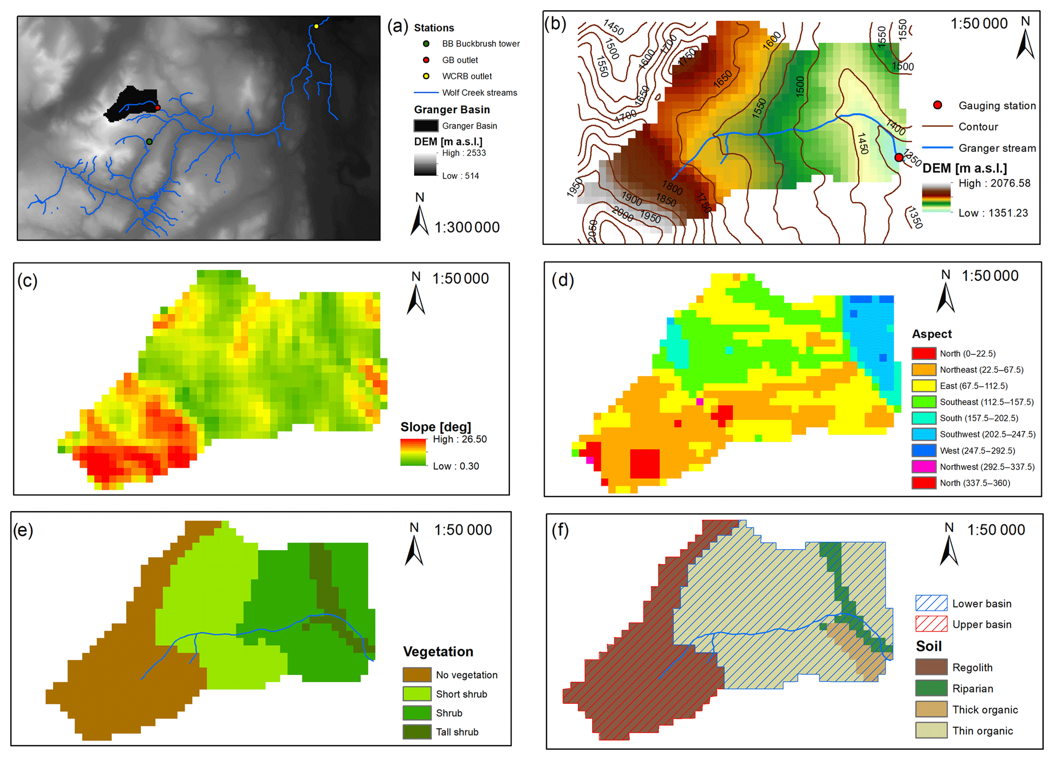
Figure 1 Granger Basin (GB) characteristics showing (a) location within the Wolf Creek Research Basin (WCRB), stream network and gauging station, (b) topography, (c) slope, (d) aspect, (e) vegetation types and (f) soil types. Lower (LB) and upper basin (UB) areas are marked.

2.2 Data

Meteorological data (air temperature – T, wind speed, solar radiation and relative humidity) were recorded every 15 min at the Buckbrush weather station (BB; 1312 m a.s.l.), located ∼2.8 km from the GB outlet in an area of WCRB with similar characteristics to GB (Fig. 1a). To fill gaps in the meteorological data, a linear regression between the Alpine weather station (1615 m a.s.l.) 6.2 km from BB within WCRB was used over the period 2008–2017 (with a R² on average >0.67; T had the best fit with R²∼0.96). T records were adjusted for altitude, assuming the moist adiabatic lapse rate of −0.006 ^∘C m⁻¹ a.s.l. (Goody and Yung, 1995). The daily precipitation time series integrated data from two precipitation gauge instruments at the BB weather station: a Geonor T-200B gauge deployed in a standard configuration with a single Alter shield and a tipping-bucket rain gauge. The challenge of measuring precipitation in these regions has been discussed by Pan et al. (2016). According to the experimental relationship suggested for WCRB, a wind factor correction has been applied to precipitation. Finally, altitude effects were considered, assuming a 0.05 % increase in the isotopic composition of precipitation for each 100 m increase in elevation. Rasouli et al. (2019) describe the elevation-dependent climatology of WCRB and the relationship between meteorological variables among the long-term weather stations used in this study.

Automated snow pillow measurements from the BB weather station were averaged to obtain a daily time series of snow water equivalent (SWE). The instrument converts weight of the snow overtop the snow pillow into SWE. Stream discharge was calculated at the outlet of GB using a rating curve updated each year. A stilling well was instrumented with a pressure transducer (Solinst Levelogger) and compensated with a co-located Solinst Barologger measuring the pressure and stage every 15 min. Manual flows were made using a SonTek Flowtracker for a range of flow conditions and with salt dilution gauging during periods when the channels were ice-covered. The loggers were in place from mid-April to October, when they were removed to prevent freezing.

Stable water isotope samples were collected from stream water, precipitation and snowmelt. Stream water isotopic composition was taken both from grab samples and an ISCO autosampler located at the gauging station of GB. The samples had an average sampling frequency of <2 d both in 2015 and 2016 during the sampling period (mid-April to October, same as the discharge measuring period). Only a few samples were collected with snowmelt lysimeters in 2015 and 2016 at different locations in the bottom valley of GB. Rainfall samples were collected using samplers adapted after Gröning et al. (2012) from different locations both in the Granger Basin and WCRB. Stable isotope ratios of δ²H (and δ¹⁸O, which was not used here) were determined using a Los Gatos Research DTL-100 water isotope analyzer at the University of Toronto. Five standards of known isotope composition, with δ²H ranging from −154 ‰ to −4 ‰, were used for calibration, in addition to periodic checks using the international standard VSMOW2. During analytical runs, samples were interweaved with standards at a ratio of 3:1. For periods when precipitation isotopes were not sampled, they were estimated via a linear regression between precipitation δ²H and T. In addition to T and precipitation time series, the precipitation isotopic composition was spatially distributed to account for altitude effects at a rate of −0.04 ‰ m⁻¹ a.s.l. for δ²H (Holdsworth et al., 1991).

Soil hydrological properties were mapped by splitting the model domain of the entire GB into two main hydropedological units, each with different properties and hydrological responses: the upper basin (UB) and lower basin (LB; Fig. 1f). The UB includes areas at upper elevations (>1650 m a.s.l.) where bare soil is classified as regolith, bedrock outcrops occur and the organic layer is absent. The LB aggregates the other soil classes comprised of organic soil of varying thickness, including riparian soil. The model domain was also divided into four classes based on vegetation properties (Fig. 1e): a tall shrub class that occurs mainly in the riparian areas of the LB, shrub at lower elevations but not in riparian areas, short shrub in areas in the central basin and no vegetation in the UB.

Table 1 Parameters and their range of variation during calibration.

3 Model development for frozen soil and thaw layer dynamics

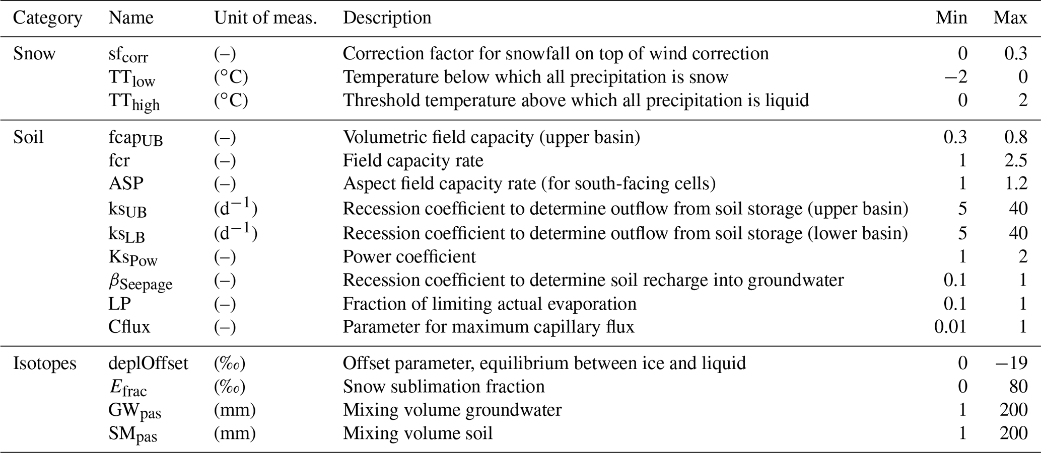
STARR is a spatially explicit hydrological model aimed at simulating water fluxes, storage dynamics, isotope ratios and water ages. It is based on a HBV-type (Hydrologiska Byråns Vattenbalansavdelning-type) conceptual structure (Lindström et al., 1997) for representing soil and groundwater storages and fluxes in terms of water flow and isotopic composition. Briefly, the model equations of the different routines (interception, snow, soil and groundwater) are applied to each grid cell. For each compartment, isotope ratios are estimated according to mixing equations with the assumption of complete mixing. The snow module is built on the assumption that the interception efficiency decreases with canopy snow load and increases with canopy density and, further, that snow unloading increases with time (Ala-aho et al., 2017a). The snow module is also energy-based; hence it accounts for the sublimation fractionation of snow isotopes both of canopy-intercepted snow and the ground-level snowpack as well as the isotopic depletion of snowmelt. Water ages are estimated by tracking the storage cell by cell at each time step, so the water ages dynamically and spatially evolves. Full details about the model structure, parameters and equations are given in van Huijgevoort et al. (2016) and in Ala-aho et al. (2017b). Here, according to the parameter sensitivity analysis conducted in previous applications of the model, some of the parameters were randomized from initial ranges and then calibrated to optimize the model in a Monte Carlo approach (Table 1). Other parameters were kept fixed to specific values selected through preliminary testing runs.

The overarching goal of STARR is to keep the model structure simple while representing the spatial distribution of dominant hydrological processes for a given environment – in this case, subarctic alpine with discontinuous permafrost. Applying the model to GB required conceptualization of the impact of frozen soil by modelling the field capacity of the soil as time-variant to represent active-layer storage (Carey and Woo, 2001b). The approach used was to (i) limit available soil storage when the soil is frozen, (ii) make available soil storage gradually increase when temperatures are above 0 ^∘C to a maximum value and then (iii) reduce available soil storage during the refreezing period (Fig. 2). The freezing dynamics were implemented by setting the field capacity (FC) to a minimum value (FC_min) when t<t₁ (where t₁ is the beginning of the thaw period) or t>t₄ (where t₄ is the end of freeze back), linearly increasing for t between t₁ and t₂ (where t₂ is the time of maximum thaw) up to the maximum value FC_max and linearly decreasing between t₃ (where t₃ is the onset of freeze back) and t₄ (Eq. 1; Fig. 2):

$$\begin{array}{}\text{(1)}& \mathrm{FC}\left(t\right)=\mathrm{FC}(t-\mathrm{1})+\mathrm{\Delta }\mathrm{FC},\end{array}$$

$$\left\{\begin{array}{l}\mathrm{FC}\left(t_{\mathrm{0}}\right)={\mathrm{FC}}_{\min }\\ \mathrm{\Delta }\mathrm{FC}=\mathrm{0},t<t_{\mathrm{1}},t>t_{\mathrm{4}},t_{\mathrm{2}}<t\le t_{\mathrm{3}}\\ \mathrm{\Delta }\mathrm{FC}=({\mathrm{FC}}_{\max }-{\mathrm{FC}}_{\min })\cdot (t_{\mathrm{2}}-t_{\mathrm{1}}{)}^{-\mathrm{1}},& t_{\mathrm{1}}\le t\le t_{\mathrm{2}}\\ \mathrm{\Delta }\mathrm{FC}=({\mathrm{FC}}_{\max }-{\mathrm{FC}}_{\min })\cdot (t_{\mathrm{3}}-t_{\mathrm{4}}{)}^{-\mathrm{1}},& t_{\mathrm{3}}\le t<t_{\mathrm{4}}\end{array}\right..$$

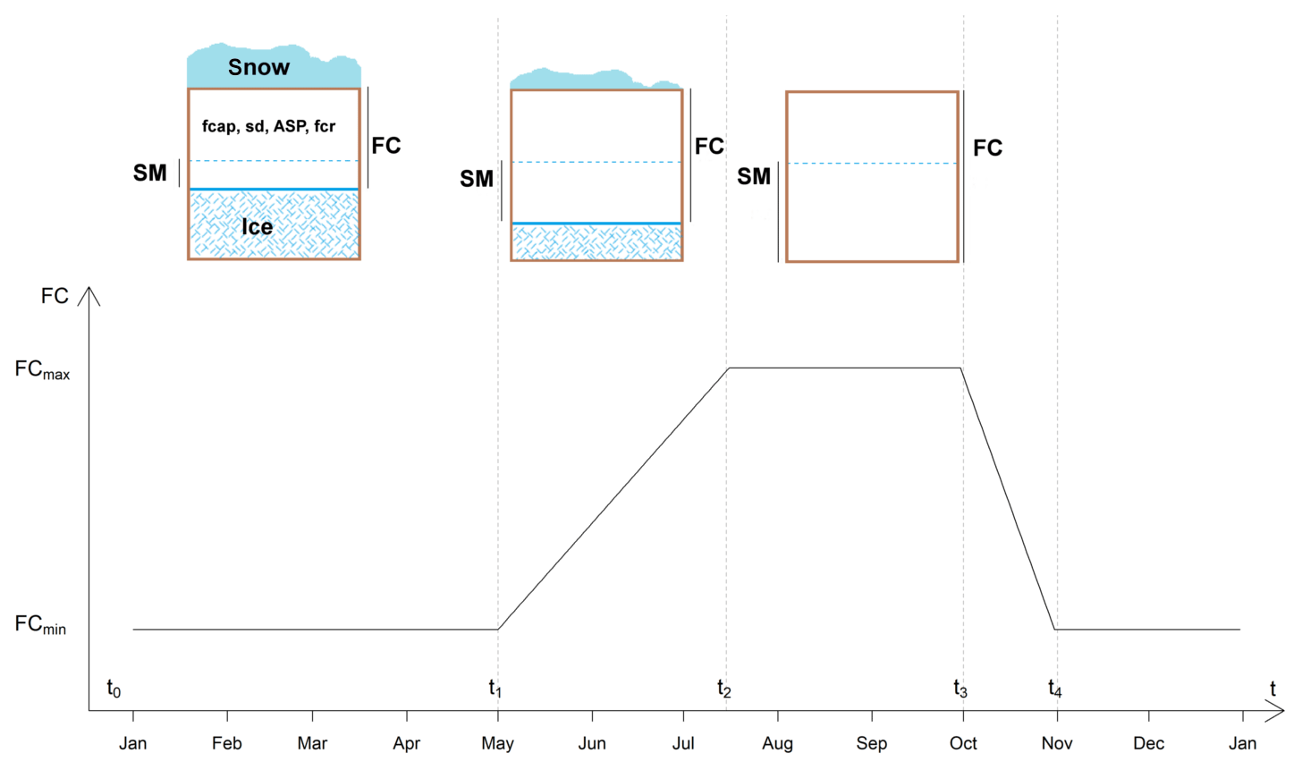
Figure 2 Field capacity (FC) parameter set to be time-variable. FC is set to a minimum value (FC_min) when t<t₁ or t>t₄, with t increasing linearly between t₁ and t₂ up to the maximum value FC_max and linearly decreasing between t₃ and t₄. The top image is a schematic representation of a soil cell to help visualize the variable FC. FC is dependent on the soil parameters: fcap (volumetric field capacity), sd (soil depth), ASP (aspect) and fcr (field capacity rate; calibrated parameter).

In addition, to make this frozen soil approximation spatially consistent with field observations, a parameter (ASP) accounting for aspect was included. Specifically, south-facing slopes were considered to have consistently higher available soil storage than the cells facing different cardinal directions. The parameter ASP was set to 1 if the cell was non-south-facing and randomly sampled from the range 1.0–1.2 for south-facing cells. This indicates that the time-variant available storage for a south-facing cell was permitted to be, at maximum, 20 % higher than a non-south-facing cell. The FC is the product of soil depth (sd) and the volumetric field capacity (fcap), and the time-variant FC is defined from FC_min (Eq. 2) and FC_max (Eq. 3):

$$\begin{array}{}\text{(2)}& {\displaystyle }& {\displaystyle }{\mathrm{FC}}_{\min }=\mathrm{sd}\cdot \mathrm{fcap},\text{(3)}& {\displaystyle }& {\displaystyle }{\mathrm{FC}}_{\max }={\mathrm{FC}}_{\min }\cdot \mathrm{fcr}\cdot \mathrm{ASP},\end{array}$$

where fcr is the field capacity rate parameter used to calibrate the ratio between FC_min and FC_max. To avoid unreasonable FC values, the fcap parameter was randomly sampled and optimized during the calibration process. For simplicity, the intervals of the piecewise function (Eq. 1) were set a priori, according to site knowledge based on previous observations of frozen ground development (Zhang et al., 2010). The endpoints were set as following: t₁ to 1 May, t₂ to 15 July, t₃ to 1 October and t₄ to 1 November. Thus, FC was set to its minimum for November–April, linearly increasing from May to mid-July, being at its maximum until October and finally sharply decreasing to represent soil freeze back. Despite most parameters values being set for the whole catchment, some were set to reflect the properties related to soil, vegetation and aspect classifications (Fig. 3).

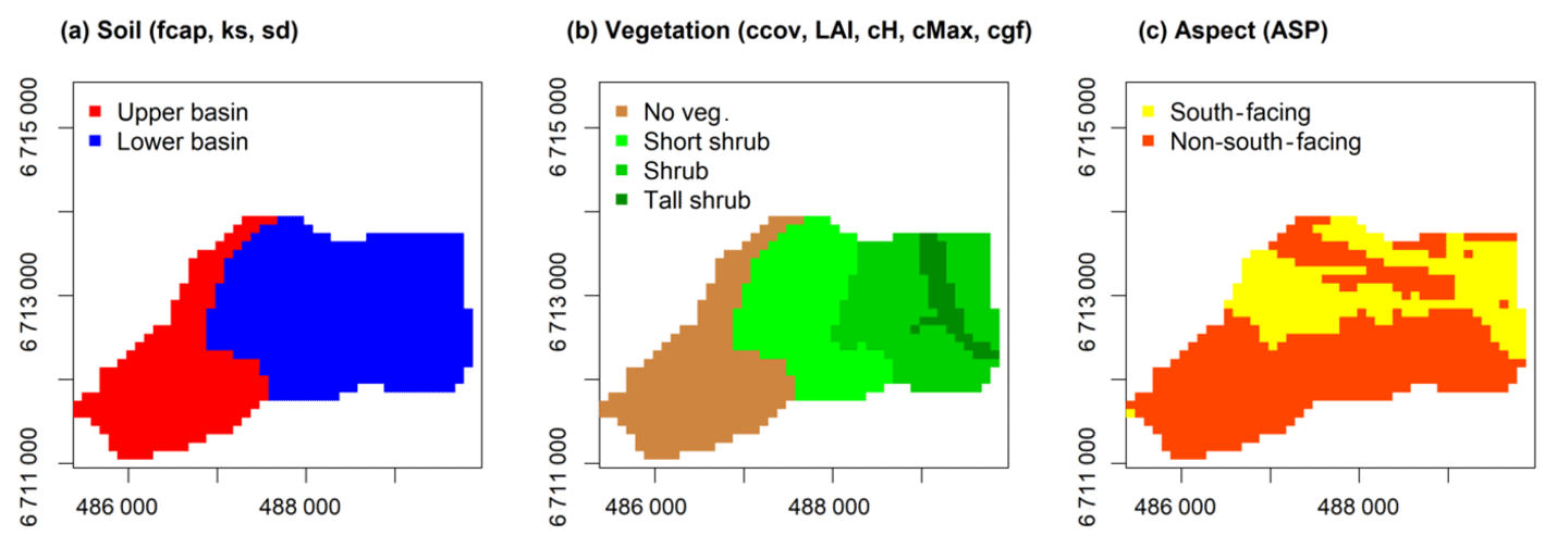
Figure 3 Aggregation used to set the spatially variable parameters: (a) soil classification for two calibrated parameters (fcap is volumetric field capacity and ks is recession coefficient) and one fixed parameter (sd is soil depth), (b) vegetation classification for five fixed parameters (ccov is canopy coverage, LAI is leaf area index, cH is canopy height, cMax is maximum canopy storage and cgf is canopy gap fraction), and (c) aspect classification for ASP parameter that was calibrated if south-facing or set to 1 for any non-south-facing aspect.

A multi-variate calibration approach (Ala-aho et al., 2017b; Piovano et al., 2018) was applied to optimize the model according to three variables: discharge, SWE and stream water isotope values. To obtain model efficiencies of discharge and stream water isotopes, we compared observations of both at the gauging station with simulated values at the outlet cell. For SWE, we compared the observed SWE at BB and the catchment average of simulated snowpack for each time step. However, the simulated values were dependent on elevation, and it was not possible to compare simulations and observations directly as measurements were taken at BB, outside of GB. We ran 7000 simulations in a Monte Carlo approach, each one being characterized by a parameter set randomly sampled from an initial range (Table 1). In each simulation, years 2014 and 2015 were looped in order to initialize the system in terms of stabilizing both water storage and isotope values. A multi-variate calibration was then conducted for the study period 1 January 2014 to 31 December 2016, and for each simulation, three efficiencies were determined: Kling–Gupta efficiency (KGE; Gupta et al., 2009) for evaluating discharge and SWE and mean absolute error (MAE) for evaluating δ²H simulations. The empirical cumulative distribution functions of these efficiencies were used to select the 100 simulations showing simultaneously the highest values of KGE for discharge and SWE and the lowest value of MAE for stream water δ²H. KGE was chosen for hydrometric variables, as it is based on equal weighting of linear correlation, bias ratio, and variability. KGE tends to be a more balanced approach than the Nash–Sutcliffe efficiency (NSE; Nash and Sutcliffe, 1970), with less biasing to peak runoff (Gupta et al., 2009). For evaluating simulation results for stable isotopes, MAE was chosen, as the error range estimates are of the same scale as observation variability and MAE provides advantages over the root-mean-square error (RMSE; i.e. MAE is a more stable measure of the magnitude of average error, while the RMSE can be confounded by the variable functional relationship between the RMSE and average error; Willmott and Matsuura, 2005). Time series results were based on the 100 best simulations, while the spatial model outputs were based on the best simulation according to the same method used for the 100 best simulations and were therefore dependent on the intrinsic characteristics of the selected simulation.

The approach used in STARR allows estimation of the spatial distribution and dynamic variation of water ages. In addition to the isotopic composition, water ages were computed according to a full-mixing assumption within each cell and time step, according to passive storage parameters for soil and groundwater reservoirs in the model (Table 1). Water ages of total runoff (i.e. overland flow and lateral soil and groundwater fluxes) were estimated using a mass balance for each cell that tracked all inflows and outflows and quantified total runoff. During each time step, water stored in each model compartment becomes a day older, with the age of incoming precipitation taken as 1 d. The age of water in each compartment evolves dynamically through mixing and water exchange between compartments and cells. Stream water ages evaluated at the outlet cell are the time-variant integration of all water fluxes from different catchment compartments, each having their own age distributions (similar to Soulsby et al., 2015). All simulations were performed at 100 m × 100 m resolution and at a daily time step.

4 Results

4.1 Temporal dynamics of water fluxes, storage and age

During the study, measured discharge ranged from 0.001 to 1.1 m³ s⁻¹ (Fig. 4). There were limited discharge measurements between October and April, except for occasional under-ice measurements. Seasonal variability in flow was more marked than the inter-annual variation (standard deviation across all years for the sampling period April–October is σ=0.139, while for each year, σ₂₀₁₄=0.147, σ₂₀₁₅=0.145 and σ₂₀₁₆=0.116). In each year, the first recorded flow peak was related to snowmelt, while later in the summer, discharge was most responsive to large rainfall events (Fig. 4a, b). In 2014, the peak discharge (1.1 m³ s⁻¹) occurred at the beginning of July, following a 36 mm rain event. In 2015 the peak was 0.67 m³ s⁻¹, recorded at the end of May during the spring melt. In 2016, peak flow (0.85 m³ s⁻¹) was measured in mid-June following a 31 mm rain event, at the end of the snowmelt period.

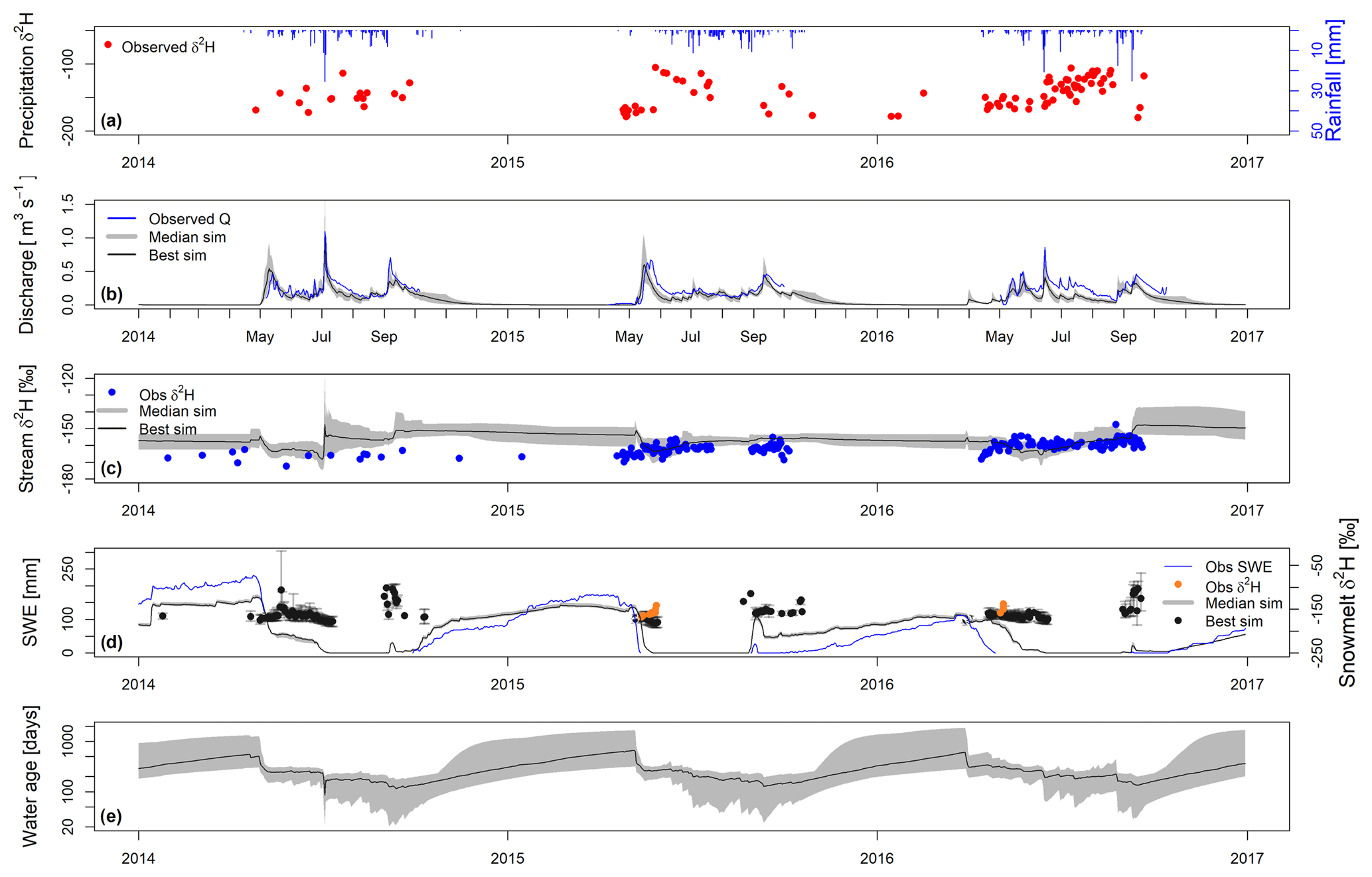
Figure 4 Time series of (a) observed precipitation isotopic signature of δ²H (‰) and observed rainfall (mm). Time series of simulated (grey) and observed (b) discharge Q (m³ s⁻¹), (c) stream water isotopic signature δ²H (‰), (d) catchment average snow water equivalent (SWE; mm) and snowmelt isotopic signature δ²H (‰), and (e) stream water ages (days) at outlet. Dark grey bands show ranges of selected best 100 runs (Best sim), and black lines are the median simulation (Median sim) among the 100 best simulations (Best sim).

Measured precipitation δ²H ranged from −76.9 ‰ to −180.2 ‰, showing seasonality with more depleted values in winter and more enriched values in summer. In contrast to the variable precipitation signal, the stream water δ²H measurements exhibited a highly damped signal that lacked the clear depression usually associated with alpine catchments during the snowmelt. If anything, δ²H shows some enrichment from the snowmelt period until the summer, albeit with some limited short-term variability (Fig. 4c). The sparse snowmelt δ²H samples were on average −155.3 ‰, which is more enriched than the minimum stream water values. The snowpack generally begins to accumulate in late August or early September, reaching a peak the following spring before the main melt period in late April to May. The highest value of the observed SWE (230 mm) was measured in April 2014 (Fig. 4d). In 2016, peak SWE was lower than in the other years (112 mm).

Given the complexity of the catchment hydrology, the model simulated the discharge dynamics quite well over the 3 years, with KGE values ranging from 0.48 to 0.70 across the 100 best simulations (Fig. 4b; Table 2). The snowmelt freshet was well reproduced, both in terms of timing and peak, yet the simulated recession limbs were slightly steeper than observed. The early summer period was characterized by the highest discharge peaks both in 2014 and 2016, which was well represented by the model. The largest underestimation of the simulated discharge was during July and August 2016 during rain-driven events. The main challenge in reproducing the stream water δ²H composition (Fig. 4c) was the limited seasonal variability of the signal, coupled with some shorter day-to-day variation. Despite the difficulties in reproducing this damped signal, the span of the efficiency across the 100 best runs (MAE between 4.41 and 5.84 ‰) was similar to the model performance obtained in previous model applications in snowmelt-driven catchments (Ala-aho et al., 2017b; Piovano et al., 2018). The simulated signal did reproduce a slight depletion after melt, followed by enrichment, although the measured melt signal showed greater seasonal mixing and damping, though greater day-to-day variation, than the simulated signal.

Table 2 Efficiency ranges of 100 best calibrations, selected to simultaneously have the highest KGE for discharge and SWE and lowest MAE for stream δ²H.

Observed and simulated temporal SWE dynamics (averaged across the catchment) are shown in Fig. 4d. The snowpack model output was highly dependent on elevation, yet the spatially averaged time series reasonably reproduced the SWE measurements, with KGEs ranging from 0.71 to 0.72 across the 100 best simulations. Overall, catchment average SWE was underestimated in 2014 and overestimated in 2016, despite capturing the peak. In 2015, the first part of the accumulation period was overestimated by the model, whereas the second part underestimated accumulation prior to melt. The melt period in 2015 was shorter than in 2016, and the decline from high values of SWE to 0 was more rapid (26 d in 2015 from early May to end of May, against 61 d in 2016 from mid-April to mid-June). Moreover, in early April 2016 the simulated melt period was interrupted by a period of refreezing, which delayed the simulated melt compared to the measured. Due to the scarcity of snowmelt isotope samples, it was not possible to include these observations in the calibration (Fig. 4d). However, simulated snowmelt δ²H was reasonable, as the majority of the observations in 2015 and 2016 fell within the uncertainty bands of the simulated composition.

Figure 4e shows the simulated stream water ages at the outlet cell of the catchment. The median water age over the calibration period was 290 d. Stream water ages showed clear seasonal dynamics: a steady increase to >1 year (with large uncertainty) when deeper sources sustained low flow periods in winter. Ages were reduced to <9 months in the early phases of the melt, gradually decreasing to around 6 months in the late summer, as younger water from melt and summer precipitation was an increasingly dominant source of runoff. The uncertainty was considerably reduced during high flow periods.

4.2 Spatial variability of water fluxes, storage and ages

Figures 5, 6 and 7 provide spatially distributed estimates of select model outputs (i.e. simulated SWE, soil storage volumes and ages of water fluxes from each cell) at hydrologically relevant dates or averaged over specific periods. The patterns in the SWE maps (Fig. 5) reflect the influence of the vegetation parametrization (e.g. presence of shrubs in the lower basin with interception and unloading processes) in addition to the influence of elevation. In 2015, the simulated snow accumulation was less variable across the catchment compared to the more heterogeneous snowpack in 2016. In 2015, melt occurred with a short time lag between lower and upper elevations (16 d difference when SWE = 0 in the lowest and highest catchment cells). In contrast, in early 2016 simulated SWE values were more heterogeneous across the catchment. Highest simulated averaged values occurred when the lower catchment had values ≤50 mm, whereas the upper basin reached 300 mm. In contrast to the rapid melt in 2015, the time lag between the day when SWE = 0 occurred at the lowest and the highest cell in the catchment was 59 d. This reflected the slower observed melt, though the modelled melt was delayed.

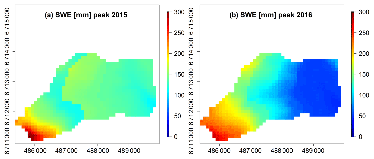
Figure 5 Spatial distribution of snow water equivalent SWE (mm) for the day of peak SWE in both study years: (a) 23 February 2015 and (b) 19 March 2016.

Spatially simulated liquid soil water storages are shown in Fig. 6 for different periods. The highest simulated values of soil water storage occurred immediately after the melt period in 2015 (Fig. 6a) and in 2016 (Fig. 6b). As the melt period was shorter and occurred more uniformly across the catchment in 2015 compared to 2016, the variability in soil storage across the cells was lower in 2015 than in 2016 (standard deviations σ=13.8 mm compared with σ=22.2 mm in 2015 and 2016, respectively). In 2016, the upper basin cells received considerable water inputs (up to 183 mm) from melt, while in the lower basin the storage was lower than 36 mm. In addition, estimated soil water storage averaged on biweekly windows provided information on the spatial variability in soil water storage, as the thaw layer increased while soils approached the highest overall field capacity (Fig. 6c and d). The highest field capacity occurred when the available storage was maximized (Fig. 6e and f) and then when available liquid storage was declining during freeze back (Fig. 6g and h). Overall, spatial patterns in the soil storage maps reflect a combination of the empirically based parametrization of aspect (south-facing and non-south-facing) as well as the distinct vegetation and soil characteristics of the upper and lower basin.

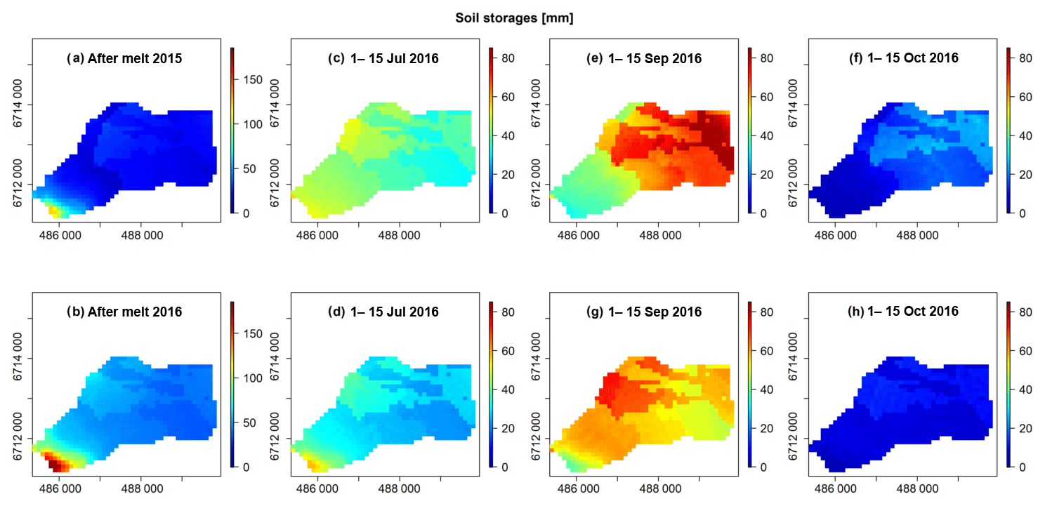
Figure 6 Spatial distribution of simulated water soil storages (mm). Daily snapshots on first snow-free day in the year: (a) 28 May 2015 and (b) 18 June 2016. Values averaged over 15 d: (c) 1–15 July 2015, (d) 1–15 July 2016, (e) 1–15 September 2015, (f) 1–15 September 2016, (g) 1–15 October 2015 and (h) 1–15 October 2016. Note that scales in (a) and (b) are different to the scales in (c).

Simulated ages of runoff (as combined overland flow and lateral flow from model cells) varied across the catchment during the period simulated (Fig. 7), according to the spatial variation of storage reservoirs and water fluxes. Deep groundwater contributions were generally negligible, consistent with the conceptual model of hydrology in GB that accounts for runoff generation occurring primarily from shallow lateral flow in the upper organic soil layers (Carey and Woo, 2001). Estimated water ages were predominantly influenced by soil runoff ages, as overland flow only occasionally occurred during melt. Overall, patterns of simulated water ages reflected flow path lengths and soil storage patterns, with ages increasing along drainage directions from hillslopes towards the valley bottom. Cells located at the convergence of the longest flow paths had modelled water ages consistently older than in the other catchment cells (usually older than 300 d). From the oldest ages immediately following melt (catchment average of 295 d for 2015 – Fig. 7a – and 233 d for 2016 – Fig. 7b), as stored water was displaced, water ages decreased with increasing soil storage, summer precipitation and discharge in July (catchment average of 242 d for July 2015 – Fig. 7c – and catchment average of 234 d for July 2016 – Fig. 7d), reaching the youngest overall ages at the end of the summer (catchment average of 177 d September 2015 – Fig. 7e – and 185 d for September 2016 – Fig. 7f). Ages increased again in October (2015 in Fig. 7g and 2016 in Fig. 7h), when the availability of soil storage became restricted as refreezing occurred. Water ages after melt were greater in 2015 than in 2016. This is consistent with the different characteristics of the snowmelt periods in the 2 years in terms of timing, magnitude and heterogeneity across the catchment. As in 2015, melting was more homogenous compared to 2016, and the day after complete snowmelt (i.e. the first day with SWE = 0 in all cells) occurred less than 1 month after highest values of SWE, the hydrological system was still affected by the mobilization of old water in storage, and the influence of newer meltwater became stronger several days later. However, the melt period in 2016 was longer with a gradual decrease in the snowpack (2 months from high values of SWE to 0), and so the model compartments had already time to be filled with newer water inputs, which made the overall age pattern younger.

Figure 7 Spatial distribution of simulated water ages (days) of runoff contributions (overland and lateral flow) from model cells. Daily snapshots on first snow-free day in the year: (a) 28 May 2015 and (b) 18 June 2016. Values averaged over 15 d: (c) 1–15 July 2015, (d) 1–15 July 2016, (e) 1–15 September 2015, (f) 1–15 September 2016, (g) 1–15 October 2015 and (h) 1–15 October 2016.

5 Discussion

5.1 How well can spatially distributed tracer-aided modelling capture thaw layer dynamics and runoff generation in permafrost catchments?

In discontinuous permafrost environments, storage dynamics and water distribution are strongly affected by the seasonal variability of frozen ground, the heterogeneity in snow accumulation and melt, and (particularly in alpine areas) the strong variability in energy receipt due to low sun angles (Quinton and Carey, 2008; Woo, 2012). There has been limited application of isotopes to investigate water sources and pathways in permafrost regions (McNamara et al., 1997; Metcalfe and Buttle, 2001; Hayashi et al., 2004; Carey et al., 2013b; Suzuki et al., 2006; Tetzlaff et al., 2018). There have been fewer studies that have used hydrological models that explicitly incorporate tracers in permafrost and snow-dominated regions (e.g. Lessels et al., 2015). Here, a spatially distributed model that integrates isotopic composition and discharge was applied to simulate runoff generation, stable isotopes, snowmelt and track water ages. By taking thaw dynamics into account, a time-variant available soil storage was implemented for the first time in STARR. Previous applications of STARR demonstrated that multiple data sets and calibration criteria helped to constrain models and provided information on the relative value of observations (Ala-aho et al., 2017b; Piovano et al., 2018), guiding experimental design and providing information on gaps in process understanding (Kuppel et al., 2018). In this work, by incorporating a simple but distributed conceptualization of thaw dynamics, STARR was able to effectively simulate the temporal dynamics of discharge with an adequate damping of the stream isotope signal. Despite the large variability in storages and fluxes – which are well-documented for GB – the model was able to efficiently simulate the three calibration variables, providing confidence that the dominant governing processes were generally well simulated and parameters well represented. That said, although the overall damping of the isotopes was captured, the detailed short-term day-to-day variation was not. Also, the model exaggerated the effect of the depleted snowmelt pulse reaching the stream.

At WCRB and GB, previous research has documented how frozen ground status, organic soils, aspect and permafrost dominate the hydrological response to rain and snowmelt events (Quinton et al., 2004, 2005; McCartney et al., 2006). In complex alpine landscapes, aspect and altitude control the timing of melt and the subsequent delivery of water to soils. Organic soils are hydrologically complex, with a high porosity that can rapidly convey water to the stream when thawed or near 0 ^∘C during melt. Lateral flow in organic soils is a key process in subarctic permafrost regions, as hydraulic conductivity is typically orders of magnitude greater than underlying mineral substrates (Carey and Woo, 1999, 2001b; Quinton et al., 2005). The descent of the frost table along permafrost slopes allows deeper flow pathways to become active even as water tables typically fall, muting streamflow response (Carey et al., 2013a). Areas without permafrost are thought to contribute less to runoff, yet the overall disposition of permafrost in alpine landscapes is difficult to fully ascertain (Bonnaventure et al., 2012) and the relative influence of deeper groundwater flow is uncertain at present. Given this complexity, the day-to-day isotope dynamics are likely underpinned by more localized spatially heterogeneous processes, which are probably not fully captured by the current model set-up (Ala-aho et al., 2017a).

This is because in this study, STARR was set up to best represent the process understanding described above by (i) splitting the model domain into two hydropedological units based on organic soil presence, (ii) including a classification based on aspect to reflect permafrost presence and available soil storage, and (iii) allowing soil storage to be time-variant to reflect the seasonal development of frozen ground. Previous research in GB highlighted the importance of spatially representing processes in both field and modelling studies. For example, for the snowmelt period, McCartney et al. (2006) divided GB into nine hydrological response units (HRUs) based on similarities in hydrological, physiographic, vegetation and soil properties. Dornes et al. (2008) showed that a distributed hydrological model based on five HRUs was necessary to describe the observed magnitudes of both snowmelt and basin runoff. In this work, we explicitly simulated processes in GB at a 100 m scale. Model results support the observations that overland flow is largely absent in this basin (Carey and Woo, 2001a; Carey et al., 2013a) and that spatially represented melt is critical in accurately predicting snowmelt freshet (McCartney et al., 2006; Dornes et al., 2008). The spatial representation of processes in GB was also important in simulating biogeochemical processes as shown in Lessels et al. (2015). However, it is likely that the 100 m grid is too coarse to pick up small-scale processes, which might affect the day-to-day isotope variability.

5.2 Spatio-temporal variations in water storage, flux and ages

Spatial heterogeneity in modelled hydrological response was most strongly influenced by the timing and magnitude of ground freeze–thaw and also by the heterogeneities of inflows from snowmelt. Simulated melt rates were highly variable among years due to the disparate nature of snow accumulation and contrasts in melt rates across elevation, vegetation type and aspect. The differential melt rates affect various aspects of hydrological response, including the distribution of soil storage, isotopic composition and water ages. STARR explicitly tracks the spatial distribution of water isotopes from melt and rainfall inputs and through the soil system to the stream. This approach provides an additional temporal dynamic of soil water ages throughout the catchment. Linking runoff generation processes to water ages is similar to, yet distinct from, hydrograph separation approaches that isolate sources of water (Laudon et al., 2002; Carey and Quinton, 2004; He et al., 2015). Other techniques for estimating water ages, such as convolution integral transit time distributions (McGuire and McDonnell, 2006), lumped conceptual models (Soulsby et al., 2015) and storage selection functions (Rinaldo et al., 2015), are useful, yet they are limited in terms of capacity to track the spatial distribution of water ages in the catchment. To our knowledge, there has been no estimate of spatially distributed water age in subarctic and arctic regions.

Simulated water ages at the end of the melt season were older than in any other season, as the main water source at this time is the stored water within the catchment which is being mixed with, and displaced by, snowmelt (Figs. 4 and 7). So the main source of water at the end of the snowmelt period is relatively old water that has been stored in the catchment over winter. The sources of water that lead to streamflow response have been previously studied in GB and other permafrost catchments using stable isotopes and more traditional hydrograph separation techniques (Quinton et al., 2005; Boucher and Carey, 2010). Conceptual models often suggest that low storage capacities and high runoff ratios observed during the freshet must be dominated by inflow from directly connected melt, or “new” water, as opposed to “old” water that resides in the catchment over winter when soils are frozen. However, empirical results have been variable, with some catchments showing a predominance of new water (Cooper et al., 1991, 1993; McNamara et al., 1997; Hayashi et al., 2004) or old water (Obradovic and Sklash, 1986; Gibson et al., 1993; Carey and Quinton, 2004; Carey et al., 2013a) depending on site characteristics and/or the time of year. While the cause of the differing new and old water contributions is unclear, there appears to be considerable inter-annual variability based on hydrological conditions of the ice-rich soil and the nature of melt (Metcalfe and Buttle, 2001; Carey et al., 2013a). In this study, water ages as determined by STARR were the oldest after melt and then decreased throughout the summer. While there was considerable variability within the catchment, this pattern generally holds until freeze back begins in October and soil storages decline. The decline in soil storage, however, represents a dynamic liquid water storage, not total water storage in soils. For GB, Carey et al. (2013a) reported event water contribution from two-component hydrograph separation ranging from 10 % to 26 %, suggesting that most of the water reporting to the outlet during freshet is old water (up to 90 %). This observation agrees well with results of STARR, suggesting that streamflow water during freshet is primarily displaced old water that has resided in the watershed over winter. This is also consistent with the findings of recent small catchment observations at Trail Valley in Canada (Tetzlaff et al., 2018) and larger-scale observations in the catchment of the Ob River in Russia (Ala-aho et al., 2018a, b).

The mechanism of old water displacement from soil storage to the stream during melt results in the mixing and dampening of the isotope signal (Unnikrishna et al., 2002). This appears to be the case in GB, where despite the presence of frozen ground and permafrost, multiple years of study suggest that pre-event water predominates, and model results presented here suggest that water is oldest during freshet. Previous model runs (Ala-aho et al., 2017a; Piovano et al., 2018) in snow-influenced catchments (in Idaho, US; Sweden; and Ontario, Canada), not affected by permafrost, showed a dominance of young soil water ages during melt, followed by a gradual increase in water ages. The difference to these previous studies suggests that the permafrost and thaw of frozen ground play a key role in the predominance of old water during freshet in GB. The question remains as to how soils that are largely frozen or at 0 ^∘C during melt can contribute old water to the stream and why the new water signal from large volumes of meltwater is strongly damped. The most plausible explanation is the presence of organic soils, which are able to mix and transmit water during melt, even at 0 ^∘C. It is also worth noting that the freshet also coincides with the “first flush” of high DOC values, underlining the mobilization of organic-rich soil waters by the melt (Lessels et al., 2015). The ability of organic-rich soil horizons to mix and dampen isotope signals has been documented in other cold environments (Tetzlaff et al., 2014). In GB, organic soils cover much of the basin, and empirical studies have shown that their high porosity allow several hundred millimetres of total water storage when saturated (Quinton et al., 2005). Depending upon their moisture content at freeze back, there may be a considerable infiltration opportunity during melt (McCartney et al., 2006). Carey et al. (2013a) hypothesized a mechanism where in the early stages of melt, there is limited transfer of water to the stream until unsaturated storage capacity is satisfied and infiltrating meltwater supplies sensible heat to bring soils to 0 ^∘C (yet not necessarily thawed). At this time, mixing with pre-meltwater occurs and runoff generation begins. It is instructive that the contribution of old water increases throughout the melt period (Carey and Quinton, 2004; Boucher and Carey, 2010), which corresponds to the age estimates from STARR. Furthermore, the differences in ages between years (Fig. 7), particularly during melt, support the observations that there is considerable inter-annual variability in the ages and source of water contributions, which are linked to conditions of the previous fall and the rate and timing of melt.

The use of STARR as a spatially distributed tracer-aided model provided a number of new insights into the hydrology of GB, which has a rich history of observation and model application. While prior work identified the dominance of old water during freshet (Carey and Quinton, 2004; Carey et al., 2013a), STARR was able to support this finding in a conceptual model that captured the dominant runoff generation mechanisms and mixing processes. The role of organic soils and variable soil storage was highlighted through multiple lines of evidence, and the importance of over-winter storage and melt dynamics on water ages was partially clarified. The implications of this enhanced understanding are important in terms of hydrological and biogeochemical response to climate change. In this region, temperatures are warming rapidly, particularly in winter (DeBeer et al., 2016). Changes in flows and biogeochemical fluxes for northern regions have been reported at larger scales (Frey and McClelland, 2009; Tank et al., 2016), yet their link to process understanding at the headwater scale remains scarce. At the larger continental scale of arctic river basins, increased temperatures have been shown to decrease in amounts of catchment water storage due to increased thaw and evapotranspiration (Suzuki et al., 2018), suggesting a gradually decreasing influence of permafrost on controlling hydrological function. This possible scenario of an accelerating hydrological cycle in cold regions requires further multi-scale investigation. At the headwater scale, the fact that there is considerable inter-annual variability in the hydrological and isotopic response suggests large potential variability in ages, which may amplify as the soil freezing regimes change. Furthermore, the influence of permafrost thaw on water ages remains unclear. Considering how water ages links to soil contact times and biogeochemical processes, further application of age estimation and understanding water storage dynamics may aid in understanding ecosystem response in a warmer world.

6 Conclusions

In this work, we applied the spatially distributed, tracer-aided model STARR to a cold, permafrost-influenced catchment in Yukon Territory, Canada. The model was subject to multi-criteria calibration with multi-year field data to simulate runoff, snowpack dynamics and stream isotope composition. The model captured all three variables reasonably well, and notably, the highly damped stream isotope signature was reproduced. Critical to this was the conceptualization of the thaw layer dynamics and thick organic soils, which provided a sufficient mixing volume that buffered the snowmelt isotope signature prior to water reporting to the stream network. Simulation results from the model output correspond with previous field investigation and hydrograph separation studies that indicate relatively old water (pre-event) dominating runoff generation during spring freshet. The relatively flashy nature of spring freshet in this largely frozen alpine catchment may seem counter-intuitive to this finding, yet water stored within the catchment from the previous year is the main source of stream water at the end of the melt season and explains isotopic damping of the signal. This result has important implications for processes that drive inter-annual variability and biogeochemical cycling, as there are considerable time lags in the system. How climate warming affects frozen ground and water ages is uncertain, yet water ages will likely increase with a reduction in the cold season. Another important conclusion is that the snowmelt regime, which is variable each year, is an important factor in controlling water ages.