the Creative Commons Attribution 4.0 License.
the Creative Commons Attribution 4.0 License.
 | 17 May 2019
The recent developments in cloud removal approaches of MODIS snow cover product
Xinghua Li
Yinghong Jing
Huanfeng Shen
Liangpei Zhang
The snow cover products of optical remote sensing systems play an important role in research into global climate change, the hydrological cycle, and the energy balance. Moderate Resolution Imaging Spectroradiometer (MODIS) snow cover products are the most popular datasets used in the community. However, for MODIS, cloud cover results in spatial and temporal discontinuity for long-term snow monitoring. In the last few decades, a large number of cloud removal methods for MODIS snow cover products have been proposed. In this paper, our goal is to make a comprehensive summarization of the existing algorithms for generating cloud-free MODIS snow cover products and to expose the development trends. The methods of generating cloud-free MODIS snow cover products are classified into spatial methods, temporal methods, spatio-temporal methods, and multi-source fusion methods. The spatial methods and temporal methods remove the cloud cover of the snow product based on the spatial patterns and temporal changing correlation of the snowpack, respectively. The spatio-temporal methods utilize the spatial and temporal features of snow jointly. The multi-source fusion methods utilize the complementary information among different sources among optical observations, microwave observations, and station observations.
- Article
(2264 KB) - Full-text XML
- BibTeX
- EndNote


Because of the high albedo, high thermal emissivity, low thermal conductivity, and water storage ability (Tait et al., 2000; Tekeli and Tekeli, 2012), snow has a significant influence on the energy balance (Robinson et al., 1993; Crawford et al., 2013), the hydrological cycle (Şorman et al., 2007; Kostadinov and Lookingbill, 2015), and climate change (Cohen and Entekhabi, 1999; Brown, 2000). In recent years, increasing attention has been focused on monitoring the spatial and temporal change of snow cover (Gao et al., 2012). The traditional in situ snow monitoring approach is conducted only sparsely and is limited due to the large gaps in both space and time (Brown and Braaten, 1998). In contrast, remote sensing data have the advantage of a wide coverage area and relatively short revisit period (Lopez et al., 2008; Zeng et al., 2013) and have been an effective and alternative supplement for in situ data since April 1960 through the Television Infrared Observation Satellite (TIROS; Singer and Popham, 1963). According to the data source, snow cover products based on remote sensing mainly include microwave-based products, optically based products, and combined products (Frei et al., 2012), as shown in Fig. 1.
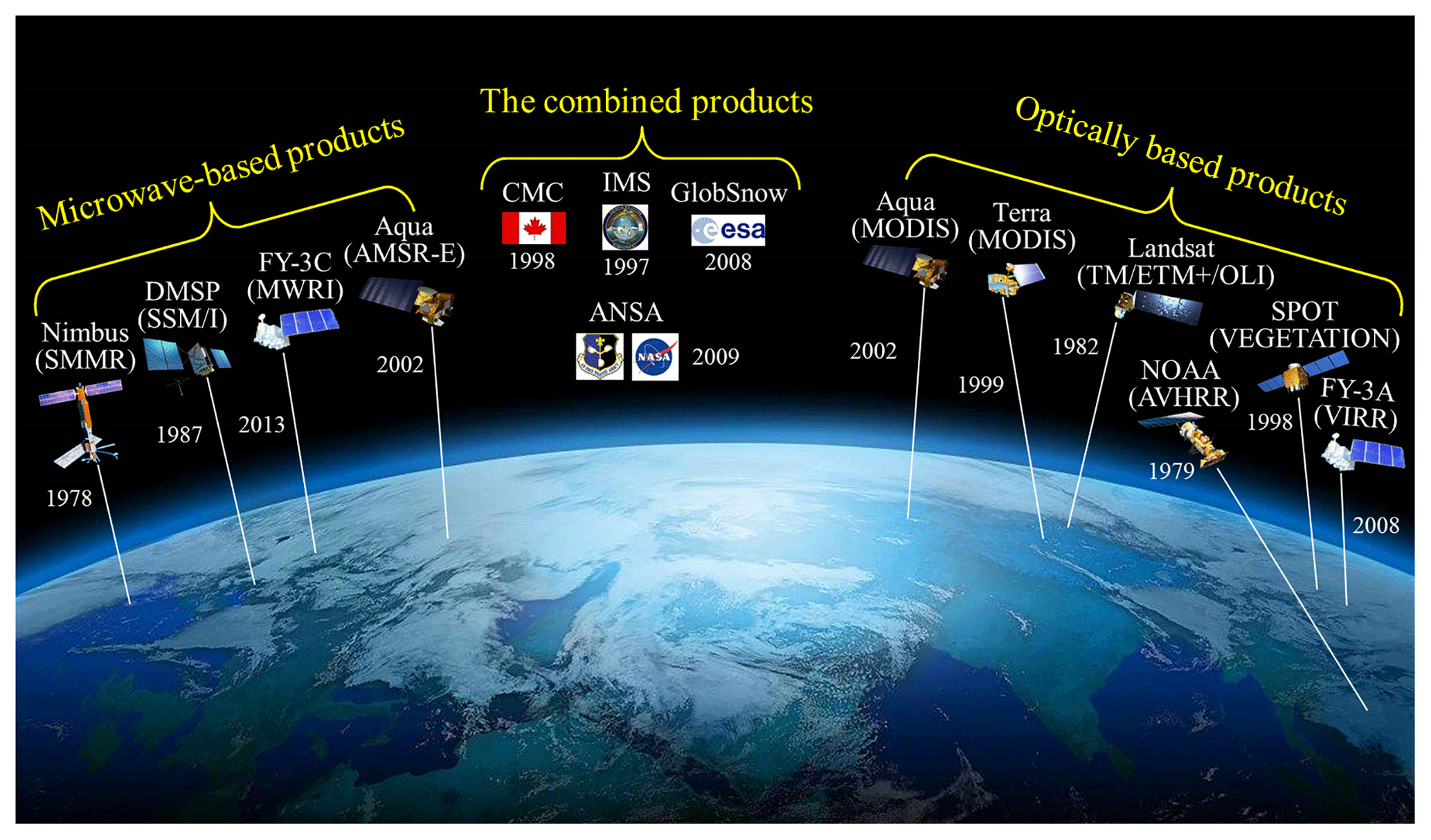
Microwave-based products are derived according to the relationship between microwave energy and snow depth (SD) or the snow water equivalent (SWE) when the snowpack is dry (Tait et al., 2000; Wulder et al., 2007). Microwave-based products are free from cloud cover contamination and can capture the snow information with an all-time and all-weather ability. Since microwaves penetrate most of the snow cover, it is possible to detect the SD and the SWE. The typical products include the Scanning Multichannel Microwave Radiometer (SMMR) SD product (Chang et al., 1987), the Special Sensor Microwave/Imager (SSM/I) SD product (Grody and Basist, 1996), the Microwave Radiation Imager (MWRI) SD product (Che et al., 2016), and the Advanced Microwave Scanning Radiometer – Earth Observing System (AMSR-E) – SWE product (Gao et al., 2010a; Anthony et al., 2008). Microwave-based products, which include both active and passive forms, have a high temporal resolution and can quickly cover the Earth's surface in 3 to 5 d. Compared to the passive microwave platform, active microwave remote sensing has a higher spatial resolution (<1 km) and can provide the details of snow cover. However, active microwave remote sensing is rarely used in research into the SD because it features a highly transparent frequency to snow (Baghdadi et al., 1997) and can only recognize wet snow reliably (Dietz et al., 2012a). In contrast, passive microwave remote sensing is effective in retrieving both the SD and SWE. However, the spatial resolution of passive microwave remote sensing systems is usually so low (>1 km) that they are not able to acquire the detailed information of snow (Foster et al., 1984). Generally speaking, passive microwave-based products are not suitable for mesoscale or micro-scale research and may result in confusion between wet snow, thin snow, and forest (Tait et al., 2000). In addition, because of the limitations of the imaging orbit gap, microwave-based products are subject to spatial gaps.
Compared to the microwave-based products, optically based products have no spatial gaps resulting from the imaging orbit gap. Optically based products are derived according to the differences in visible and infrared spectra between snow and cloud, bare land, and vegetation. The representative products are mainly derived from the Moderate Resolution Imaging Spectroradiometer (MODIS) sensor onboard the Aqua and Terra satellites (Hall et al., 2002), AVHRR data (Simpson et al., 1998), VEGETATION data (Xiao et al., 2004), Thematic Mapper (TM) data (Rosenthal and Dozier, 1996), Enhanced Thematic Mapper Plus (ETM+) data (McFadden et al., 2011), Operational Land Imager (OLI) data (Crawford, 2015), and Visible and Infrared Radiometer (VIRR) data (Zhang et al., 2017). Moreover, the weekly snow cover product (Brown et al., 2010) from NOAA is also derived from optical remote sensing imagery. The optically based products have formed long observation time series (from 1960) and have a high spatial resolution (≤1 km). The unique spectral signature (e.g., high albedo or high thermal emissivity) of snow derived from optical observations is commonly used in the snow cover mapping algorithms (Simic et al., 2004). Optical observations can also be used to extract useful snow information. For example, the snow cover area (SCA) or snow cover extent (SCE) is usually extracted by binary classification or the use of the subpixel snow-fraction algorithm with the optical observations (Rittger et al., 2013; Salomonson and Appel, 2004). The optically based products can not only be applied for monitoring the spatio-temporal variation of snow cover but can also be set as the input of atmospheric forecast and hydrological models. As a result, the optically based products are widely used in practical applications. However, they are inevitably subject to cloud cover contamination. Especially in the snow period, the cloud fraction of snow product is usually more than 10 % (Liang et al., 2008b).
In order to derive cloud-free snow cover products, combined products are generated, which are combinations of satellite data (optical and microwave), climate station observations, and models (Frei et al., 2012; Tait et al., 2000). For example, the Canadian Meteorological Centre (CMC) snow product (Drusch et al., 2004) is a combination of station observations and models, and GlobSnow (Metsämäki et al., 2015), from the European Space Agency (ESA), is a multiple-dataset snow cover product generated from satellite data, station observations, and models. In addition, the Interactive Multisensor Snow and Ice Mapping System (IMS) produced by the US National Ice Center (NIC; Ramsay, 1998) is the fusion of many kinds of optical and microwave data, including Advanced Very High Resolution Radiometer (AVHRR) data, SSM/I data, AMSR-E data, Geostationary Operational Environmental Satellite (GOES) data, Polar Operational Environmental Satellite (POES) data, european geostationary meteorological satellite (METEOSAT) data, Japanese Geostationary Meteorological Satellite (GMS) data, the National Centers for Environmental Prediction (NCEP) model data, US Air Force (USAF) snow and ice analysis data, and so on. The IMS is also jointly supported by the US National Oceanic and Atmospheric Administration (NOAA), the US Navy, and the US Coast Guard. Regardless of cloud cover, the IMS produces near-real-time products with spatial resolutions of ∼1, ∼4, and ∼24 km, which provide the input for atmospheric forecast models (Brown et al., 2014). In addition, the Air Force Weather Agency (AFWA) and National Aeronautics and Space Administration (NASA) snow algorithm (ANSA) blends AMSR-E, MODIS, and Quick Scatterometer (QuikSCAT) data products (Foster et al., 2011). Since ANSA integrates optical, passive, and active microwave data, it can map the snow-covered area (SCA), the fractional snow cover (FSC), the SWE, and the snowmelt area. The combined products draw together the respective advantages of each of the component products to improve the accuracy, quality, and spatio-temporal continuity of snow cover. Several problems encountered when the component products are used alone, including cloud cover and low accuracy, have been solved. The combined products provide more information on the state of snow cover than each of the component products. However, the primary disadvantage of the combined products is the poor spatial resolution (>1 km; Tait et al., 2000).
Although the combined products have the advantage of spatio-temporal continuity, they need many different data sources, and their spatial resolution is restricted to the lowest spatial resolution among the data sources. As a result, many attempts have been made to derive spatio-temporally continuous snow cover products from optical remote sensing data. Among the existing optically based snow cover products (e.g., AVHRR, VEGETATION, and VIRR), the MODIS products have become one of the main data sources for ice and snow research. The MODIS products have advantages in the spatial and temporal resolutions, global coverage, long time series, and free access, which together allow real-time, accurate, and large-area snow cover variation monitoring. The MODIS products are available through the National Snow and Ice Data Center Distributed Active Archive Center (NSIDC DAAC). The snow cover products of MODIS are derived from the SNOMAP algorithm (Hall et al., 1995). SNOMAP automatically uses the normalized difference snow index (NDSI) and decision strategies to identify snow cover (Hall et al., 2002), which makes this type of snow product more consistent with station observation data and other higher-spatial-resolution remote sensing data (Parajka and Blöschl, 2006; Wang et al., 2008; Bitner et al., 2002; Klein and Barnett, 2003; Chelamallu et al., 2014; Huang et al., 2011). According to accuracy assessments, under clear-sky conditions, the overall accuracy (OA) of MODIS snow cover products ranges from 85 % to 99 % (Parajka et al., 2012), and the overall absolute accuracy is ∼93 % (Hall and Riggs, 2007). Version 5 of MODIS snow cover products provides a binary product and a fractional snow product (Rittger et al., 2013; Li et al., 2018). The binary product is the SCA and the fractional snow product is the FSC, which are both derived from the NDSI (Singh et al., 2014; Liang et al., 2017). The SCA can be used to estimate the regional snow resource when combined with the SWE, and the FSC is a very important parameter for estimating the SWE (Molotch and Margulis, 2008). The MODIS products have temporal resolutions of 1 to 8 d and 1 month and spatial resolutions from 500 m to 0.05∘ (Déry et al., 2005). Like other optically based products, the MODIS products are prone to contamination by a large percentage of cloud cover (Wang et al., 2009; Maskey et al., 2011), which limits the continuity of snow cover monitoring in space and time. Cloud cover also causes confusion in snow discrimination (Ault et al., 2006). As a result, it is of importance to remove the cloud coverage from the MODIS snow cover products.
In the past decades, there have been a large number of algorithms developed to improve the spatio-temporal continuity of the MODIS SCA products. The SCA products are usually just classification data, so the cloud removal method is notably different from the methods for traditional remote sensing images (Li et al., 2016; Shen et al., 2015; X. Li et al., 2014). In this review, we comment on the recent developments in producing cloud-free MODIS snow cover products (without any special instructions, the product is MODIS SCA). The algorithms for generating cloud-free MODIS snow cover products are mainly categorized into temporal methods, spatial methods, spatio-temporal methods, and multi-source fusion methods.
The remainder parts of this paper are arranged as follows. Section 2 introduces the spatial methods for generating spatio-temporally continuous snow cover products. The temporal methods, spatio-temporal methods, and multi-source fusion methods are then introduced in Sects. 3–5, respectively. Section 6 summarizes the current validations and evaluations of the cloud removal methods for MODIS snow cover products. Section 7 exposes the future direction. Finally, the conclusions are provided in Sect. 8.
The spatial methods remove the cloud cover of the snow product based on the spatial patterns of the snowpack. The main spatial methods are the spatial filter (SF), the snow line mapping (SNOWL) approach, and the locally weighted logistic regression (LWLR).
2.1 The spatial filter (SF)
The most common spatial method is the SF (Gafurov and Bárdossy, 2009; Parajka and Blöschl, 2008; Paudel and Andersen, 2011), where the idea is to replace a cloudy pixel using the four or eight neighboring non-cloud pixels. There have been many rules put forward to replace the cloudy pixel, as follows: (1) the cloud pixel should be reassigned as a snow pixel on the condition that three of its four direct “side-bordering” neighboring pixels are snow (Paudel and Andersen, 2011; Lindsay et al., 2015). (2) The cloudy pixel is replaced by the main classification (land or snow); i.e., the class of the majority of the non-cloud pixels in a neighborhood is used to replace the cloudy pixel (when there is a tie, the cloudy pixel is replaced by snow; Parajka and Blöschl, 2008; Tong et al., 2009a, b). (3) Gafurov and Bárdossy (2009) proposed that when the eight neighboring pixels with a lower elevation than the cloudy pixel are covered by snow, the cloudy pixel should be labeled as being snow covered. (4) López-Burgos et al. (2013) replaced the cloudy pixel based on the elevation and aspect; that is, if any neighboring pixel has snow cover and has the same aspect and a lower elevation, then the cloudy pixel is classified as snow. In some cases, the same cloudy pixel may be labeled as snow or no snow by applying different rules. Therefore, the most suitable rule should be chosen according to the regional snow cover change rule.
The SF is usually effective for small-area cloud cover, and cloud with a proportion of no more than 10 % can be removed. For example, the SF in an eight-neighborhood pixel decreases the cloud coverage of MODIS products by 7 %, and the decrease in OA is just 0.7 % (Parajka and Blöschl, 2008). According to practical application, the SF is not very sensitive to the size of filter window (Zhou et al., 2005). Additionally, in mountainous regions, the elevation is assumed to be the dominant factor affecting the snow cover distribution. Due to the complicated topography, the accuracy of the SF usually declines with rising elevation (Tong et al., 2009b).
2.2 The snow line mapping approach (SNOWL)
The SNOWL method (Parajka et al., 2010; Dietz et al., 2013), which is also called the snow transition elevation method (Gafurov and Bárdossy, 2009; Shea et al., 2013), reclassifies the cloudy pixels as snow or land according to the elevation distribution characteristics of the snowpack. The cornerstone of SNOWL is the snow line and the land line. The snow line is the snow-covered elevation where all pixels above it are covered by snow, and the land line is the minimum elevation where snow exists (Krajčí et al., 2014, 2016; Lei et al., 2012). On that account, all the cloudy pixels above the snow line are labeled as snow, and all the cloudy pixels below the land line are labeled as land by SNOWL. The cloudy pixels between the snow line and land line are labeled as partial snow. However, the partial snow brings some uncertainties to the monitoring of snow cover variation.
SNOWL is relatively simple and easy to implement and performs well in both high and low elevations. In order to make sure that the snow line and land line are accurately labeled, the product should be at least 70 % cloud free (Gafurov and Bárdossy, 2009). Generally speaking, as the cloud fraction increases, the accuracy of cloud removal decreases. Some scholars considered aspect, topography, and land cover classes to improve the accuracy of SNOWL (Paudel and Andersen, 2011; Da Ronco and De Michele, 2014a). In a few special cases, the snow line for the whole area is hard to find, so the regional snow line for the local area is labeled (Parajka et al., 2010). In the Trans-Himalayan region, the improved regional SNOWL method removes 38.28 % of the cloud, and the misclassification error is less than 2 % (Paudel and Andersen, 2011).
2.3 Locally weighted logistic regression (LWLR)
For the LWLR method (López-Burgos et al., 2013), the snow cover probability of the cloudy pixel is predicted by the topographic and spatial relations with its neighboring cloudless pixels. LWLR uses two explanatory variables of elevation and aspect for snow occurrence probability. The information of the neighboring pixels is inversely weighted with distance and is fit to a logistic curve. The pixels closer to the cloudy pixel are assigned with a heavier weight than those that are farther apart. Finally, the estimated snow probability by LWLR is converted to a binary result according to a selected threshold. However, the method for choosing a better threshold to obtain a binary result needs more tests, and its high cost (>20 h in the Salt River basin in Arizona) limits its application to some degree. Experiments demonstrated that the LWLR method could reduce the cloud obscuration by 93.8 % in the Salt River basin in Arizona (López-Burgos et al., 2013).
Among all the spatial methods, the computational complexity of LWLR is the highest. The spatial methods mainly depend on the spatial patterns of the snowpack to reclassify the cloudy pixels. For the majority of the spatial methods, the core idea is to utilize neighboring cloud-free pixels. However, when the cloud fraction is high, the accuracy will decrease.
The temporal methods reclassify the cloudy pixels according to the temporal correlation and change rule of the snow cover. According to the time span of the product used, the temporal methods are mainly classified as the Terra and Aqua combined (TAC) method and temporal filters. The reason why the TAC method is considered to be a kind of temporal method, in our opinion, other than the multi-source fusion, is that the Aqua and Terra satellites are both equipped with MODIS (of nearly the same design). Their combination amounts to a composite of MODIS at different times.
3.1 Terra and Aqua combined (TAC)
Among the temporal methods, the TAC method is the simplest and most straightforward method. Since cloud coverage is very variable in a few hours, the TAC method (Parajka and Blöschl, 2008; Xie et al., 2009; Wang and Xie, 2009; Mazari et al., 2013) has become the most popular temporal method. The TAC method can decrease the cloud coverage ratio by 5 %–20 % without significantly sacrificing accuracy of the products. This method blends the same-day MODIS snow products on a pixel basis. If a pixel is cloudy in one product and cloud-free in another product, the cloudy pixel will be updated by the classification of the cloud-free pixel. The combination usually has the following priority scheme: snow > no snow > cloud.
The basic assumption of the TAC method is that complete snowmelt and snowfall did not occur during the time interval. In the process of merging the two products, they are considered to be identical. In fact, the Terra and Aqua products still have some small differences, for the following reasons. The first is that they are acquired at different times (3 h). The second is that most of the detectors in Aqua MODIS band 6 failed (Shen et al., 2014). In the early days (before 2012), the snow mapping method for Aqua used band 7 as a substitute for band 6; later on, Aqua MODIS band 6 was restored by the quantitative image restoration method (Gladkova et al., 2012) with a high degree of accuracy. Even so, the two products still have slight differences. According to the ground observations, the TAC method inherits the reclassification errors of the input data of Terra and Aqua (Xia et al., 2012). Gao et al. (2010b) confirmed that the TAC method can reduce the cloud cover by 5 %–14 % and 8 %–12 % at the yearly and monthly scale, respectively, and the OA is 89.7 %, which is lower than MOD10A1 by 0.7 % and higher than MYD10A1 by 1.4 %.
3.2 Temporal filters
Another popular kind of temporal method is the temporal filter methods (Parajka et al., 2012; Hori et al., 2017), which mainly include adjacent temporal deduction (ATD), multi-day combination (MDC), season filter (SFil), and temporal interpolation using a mathematical function. The first three kinds of methods are applied to the SCA product (as shown in Fig. 2), and the last method is suitable for the FSC product. It should be noted that temporal filters are also referred to as temporal interpolation methods in some literature (López-Burgos et al., 2013; Hüsler et al., 2014).
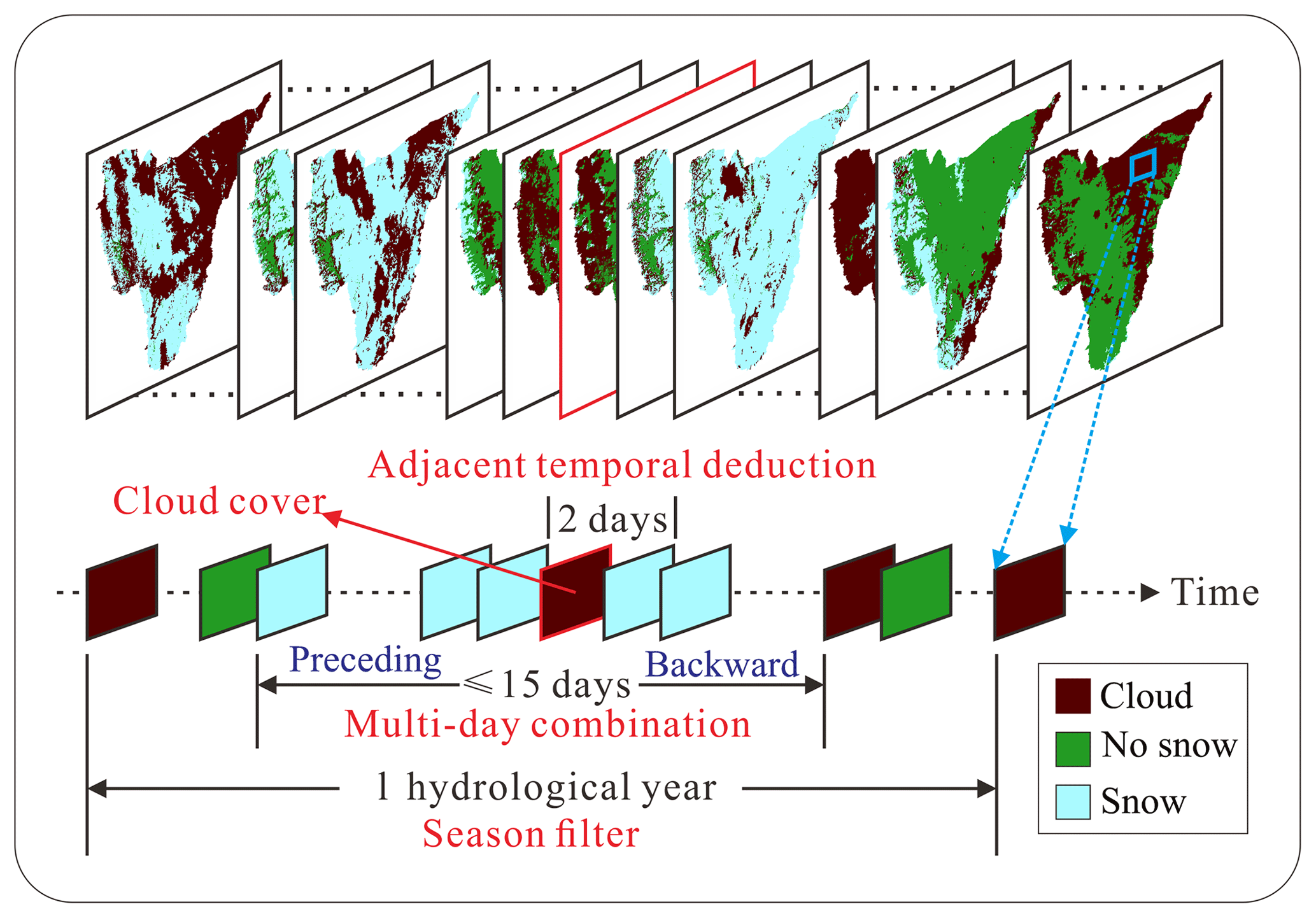
3.2.1 Adjacent temporal deduction (ATD)
ATD (Paudel and Andersen, 2011; Lindsay et al., 2015; Dietz et al., 2013) is an effective way to deduce the surface conditions via the same pixel in the previous and subsequent days without reducing the spatial and temporal resolution. It is assumed that if the preceding and the following day of the cloudy pixel remain the same (land or snow), the condition of the cloudy pixel will remain unchanged (Gafurov and Bárdossy, 2009). When the previous and the next day are different, the cloudy pixel is still labeled as cloud. In fact, ATD uses ±1 d information and is similar to the works of Li et al. (2008) and Gafurov and Bárdossy (2009), who used ±1 or ±2 d information. However, ATD is different from direct temporal replacement (Zhao and Fernandes, 2009), with the sacrifice of the 1 d temporal resolution.
Owing to the useful information from the previous day and the subsequent day, the accuracy of cloudy pixel reclassification is high. On the basis of the TAC method, ATD can not only decrease cloud fraction by 25 % but can also achieve an accuracy of 96.3 % (Gafurov and Bárdossy, 2009). However, since the snow cover is assumed to remain unchanged in the given temporal interval, the accuracy in snow-transitional periods is obviously lower than that in snow-stable periods (Gao et al., 2010b). In other words, ATD is not suitable for a context with variable snow covers.
3.2.2 Multi-day combination (MDC)
Among the temporal filter methods, MDC (Parajka and Blöschl, 2008; Dietz et al., 2012b; Zhang et al., 2012; Gao et al., 2011a) is the most widely used method. The cloudy pixels are replaced by the cloudless pixels in a temporal interval ranging from 1 d to more than 10 d with a constant or flexible way (Chen et al., 2014). For example, given a temporal window of 10 d, the constant way of MDC means that the combination is implemented in 10 d, and the flexible way represents how the combination can be implemented in varying days (≤10 d). To some degree, the above-mentioned ATD can be regarded as a special case of MDC. As far as MDC is concerned, the temporal window can be preceding (Wang et al., 2014) or preceding and backward (Sharma et al., 2014; Foppa and Seiz, 2012; Coll and Li, 2018). Usually, priority is given to the preceding days (Marchane et al., 2015). For the preceding temporal window, it amounts to a backward temporal filter in which the cloudy pixel is replaced by the previous cloud-free pixel in turn. The cloud-gap-filled method (Hall et al., 2010) also belongs to this scenario. When the land cover is considered to be unchanged, the information of the next 2 d and the previous 2 d can be used (Gafurov and Bárdossy, 2009; Da Ronco and De Michele, 2014a). To improve the accuracy of the cloud removal, certain thresholds (e.g., cloud percentage and the number of composite days) should be imposed in MDC (Gao et al., 2010b).
MDC can reduce a high fraction of cloud coverage. On the one hand, as the temporal window increases, the temporal resolution and accuracy of the result will decrease (blur). For example, it has been demonstrated that the accuracies of the 2, 4, 6, and 8 d combinations are 89.5 %, 89.0 %, 88.2 %, and 87.8 %, respectively (Gao et al., 2010b). On the other hand, the remaining cloud cover will decrease with the increase of the temporal window span. Hence, it is a trade-off between the remaining cloud and the blurring of the snow information (Hüsler et al., 2014). The longer temporal window also corresponds to a larger area of snow cover. Thus, a balance between temporal resolution and SCA should be considered. When cloud covers the pixel for more than the temporal window, MDC does not work. In this situation, the remaining cloudy pixels should be processed by other methods.
3.2.3 Season filter (SFil)
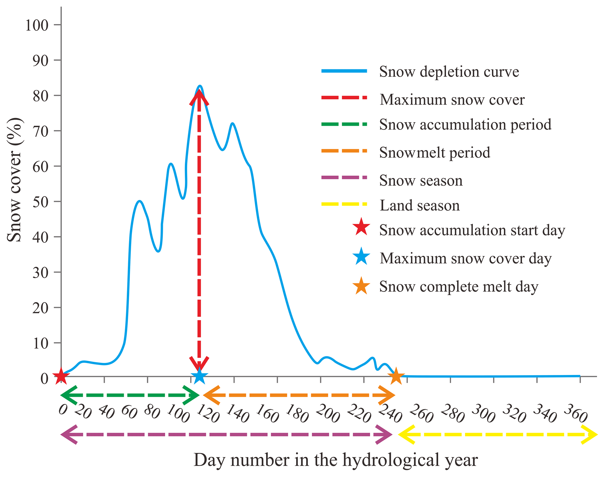
Among the temporal methods, SFil (Gafurov and Bárdossy, 2009; Gafurov et al., 2013; Lindsay et al., 2015) uses the longest time-series information to reclassify the cloudy pixels. This method needs two thresholds in one unbroken hydrological year: a complete snowmelt day and snow accumulation start day. As shown in Fig. 3, the complete snowmelt day is the day when the pixel is no longer covered by snow, and the snow accumulation start day is the start day when the snow accumulates. The hydrological year is divided into a land season and a snow season by SFil (Da Ronco and De Michele, 2014a). For example, the cloudy pixels before the snow accumulation start day and after the complete snowmelt day are in the land season, and they will be reclassified as land.
SFil can remove all the cloud cover; however, it does not take the phenomenon of more than one snow cycle occurring in 1 hydrological year into consideration. Thus, three thresholds are introduced in each hydrological year (Paudel and Andersen, 2011): the maximum snow extent day, the minimum snow extent day, and snow accumulation start day. In this way, the improved SFil effectively increases the accuracy. Similarly, Lindsay et al. (2015) defined two snow seasons: the full snow season and the continuous snow season. The full snow season is the period between the first day and the last day of snow cover, and the continuous snow season has snow cover for at least 14 d, with intervening snow-free periods of no more than 2 d. Since the short-term snowfall or snowmelt is not considered by SFil, it is often applied after other spatial or temporal methods. On the whole, SFil obtains a slightly lower accuracy than other temporal filter methods.
3.2.4 Temporal interpolation using a mathematical function
As stated previously, ATD, MDC, and SFil are applied to the binary MODIS product, and very little attention has been paid to the FSC product. For example, Tang et al. (2013) filled the cloud-contaminated pixels by cubic spline interpolation with the cloud-free observation pixels, and the mean absolute error was less than 0.1. This method is based on the the features of cloud that are rapidly changing and shift daily. In order to distinguish it from the temporal interpolation of SCA products, the temporal interpolation for FSC products is called temporal interpolation using a mathematical function, which involves interpolating the cloudy information of the FSC product along the temporal dimension of the same pixel (Tang et al., 2013, 2017; Xu et al., 2017).
In summary, the temporal methods make use of the cloud instability and the snow correlation in time. They can effectively reduce the cloud cover, partly or completely, and the accuracy is high. ATD and MDC (with time series that are not long enough) cannot reduce the cloud cover completely and may neglect short snowfall events. SFil can remove the cloud cover completely. However, when the cloud cover exists persistently in a region, the accuracy of the temporal methods will decrease. For the FSC products, temporal interpolation using a mathematical function is effective (Tang et al., 2017).
Although the spatial methods and temporal methods remove the cloud with a high accuracy, the majority of them cannot reduce the cloud completely. In order to minimize the extent of the cloud cover, many scholars have come up with spatio-temporal methods to use the complementary advantages of the temporal methods and spatial methods. This type of method relies on the correlations of snow cover in space and time with two basic forms. One is to utilize the spatial and temporal information step by step, usually as a multi-step combination method (Parajka and Blöschl, 2008; Da Ronco and De Michele, 2014b; Gurung et al., 2011; Zhou et al., 2013; Şorman et al., 2019). The other is to utilize the spatial and temporal information simultaneously (Li et al., 2017; Xia et al., 2012; Huang et al., 2018; Poggio and Gimona, 2015), which we call one-step utilization.
4.1 Multi-step combination
Multi-step combination combines the spatial methods and temporal methods alternately (Dariane et al., 2017). Although the spatial methods or temporal methods are not able to remove cloud absolutely, their successive combination can make a difference. By removing cloud progressively in each step, an accumulated cloud-free result can be obtained by multi-step combination. In other words, attempts at further reducing the residual cloud in the result of the previous step are made in the next step. Among the combined multiple steps, the TAC method is the first step in most cases. SF, SNOWL, and temporal filters are then applied in a variety of ways.
For example, a three-step method of TAC, the SF, and the temporal filter in turn was proposed (Parajka and Blöschl, 2008). Gafurov and Bárdossy (2009) proposed six steps of TAC, MDC, SNOWL, the SF with direct side-border neighboring pixels, the SF with eight neighboring pixels, and SFil. Paudel and Andersen (2011) proposed a five-step approach of TAC, ATD, the SF with four neighboring pixels, SNOWL, and SFil. López-Burgos et al. (2013) proposed a four-step combination of TAC, temporal filter, the SF, and LWLR. Da Ronco and De Michele (2014a) proposed the five-step method of TAC, the conservative temporal filter, SNOWL, the 6-day backward temporal filter, and SFil.
Whatever the combination of spatial methods and temporal methods, multi-step combination independently utilizes snow correlations in space and time, and the result from the previous step directly influences the next step. The combination order of the multiple steps is determined by their respective characteristics. For example, SNOWL requires the cloud fraction to be less than 30 %, which can be satisfied after the use of the TAC method and other temporal methods. As a result, SNOWL is often applied immediately after these methods. No matter what the combination, multi-step combination needs to adopt a feasible strategy based on the topographic features, temporal variation, and spatial heterogeneity of the snow cover. At the same time, a trade-off exists between the accuracy and the cloud fraction for the various steps. These simple multi-step combination methods have been proven to be effective and efficient in cloud reduction and agree well with station observations (Paudel and Andersen, 2011). However, this independent and successive utilization cannot take full consideration of the spatio-temporal information.
4.2 One-step utilization
In contrast, one-step utilization utilizes the spatio-temporal information simultaneously, rather than step by step. As we know, to date, most attention has been paid to the multi-step combination methods. It is only in the last few years that efforts have been made with one-step utilization methods. The one-step utilization methods are introduced in the following.
Xia et al. (2012) first introduced variational interpolation (Shen and Zhang, 2009) from the image processing field to construct a three-dimensional implicit function with five consecutive daily images (space–time manifold), which has an advantage over representing the complicated surfaces in high-dimensional spaces. The shape of the snow boundary can be easily obtained by the implicit function. It is a good case of utilizing the snow cover evolution with continuity in space and time. The results indicate that variational interpolation can maintain a close accuracy to the original product. However, its computational efficiency needs to be improved, since it intends to retrieve the space–time surface of snow cover on consecutive days.
The cloud-filling method (Poggio and Gimona, 2015) is a hybrid of the generalized additive model (GAM) and the geostatistical space–time model. The multi-dimensional spatio-temporal GAM models the binary variables, and geostatistical kriging accounts for the spatial details. The space–time correlations of snow cover are well exploited by the cloud-filling method. Even for a high fraction of cloud cover, the cloud-filling method still achieves a satisfactory accuracy and is suitable for the seasonal variation of snow cover. However, the requirement for a lot of ancillary data (e.g., land surface temperature, land cover, and soil pattern data) limits its application to some degree.
The adaptive spatio-temporal weighted method (ASTWM; Li et al., 2017) estimates the cloudy pixel according to the probability of snow cover, which is the adaptively weighted combination of the snow probabilities in space and time. Experiments demonstrated that the ASTWM not only removes the cloud completely but also achieves a high OA of above 93 % under different cloud fractions. However, the ASTWM resorts to the optimal weight of spatial and temporal probability with a high cost, and it may be able to reclassify snow cover as not being snow cover under darker conditions (Krajčí et al., 2014).
Combining the spatio-temporal–spectral information and environmental relation, Huang et al. (2018) proposed a spatio-temporal model based on the hidden Markov random field (HMRF). The information of the cubic spatio-temporal neighborhood is effectively utilized by the HMRF-based method. The snow mapping accuracy of HMRF-based method can reach 88 % and decrease the cloud cover to 1 %, which improves the overall snow mapping accuracy and reduces the omission error of the original product. For the challenging task of snow cover mapping in the transition periods of snow and in forest areas, it also obtains promising results.
Recently, increasing spatio-temporal methods have been proposed to alleviate cloud cover. In fact, multi-step combination has a numerical advantage over one-step utilization. Multi-step combination usually makes an assurance of removing the whole cloud by successive multiple steps. In contrast, one-step utilization achieves this goal in one step. One-step utilization jointly utilizes the spatio-temporal information from the snow coverage, which contributes to more promising cloud removal results.
The above-mentioned three types of methods mainly use the spatial and temporal information of the snow cover from the same optical remote sensing sensor. In contrast, multi-source fusion methods (Romanov et al., 2000; Gao et al., 2010a; Yu et al., 2012; Gafurov et al., 2015; Wang et al., 2015; Dong and Menzel, 2016) utilize the complementary information among different sources (Shen et al., 2016), such as optical observations, microwave observations, and station observations.
5.1 Optical and microwave observations
In general, optically based products have a high spatial resolution and are influenced by cloud cover, whereas microwave-based products have a low resolution and a good cloud-penetrating capacity. Therefore, the fusion of optical and microwave data has been the most representative multi-source fusion method of cloud removal, e.g., MODIS and AMSR-E (Liang et al., 2008a; Gao et al., 2011b; Akyurek et al., 2010; Huang et al., 2014, 2016; Deng et al., 2015; H. Li et al., 2014; Bergeron et al., 2014), GOES and SSM/I (Romanov et al., 2000), and the visible/infrared spin–scan radiometer (VISSR) and microwave radiation imager (MWRI; Yang et al., 2014).
The fusion of MODIS and AMSR-E is the most frequently used method. For the AMSR-E SWE product, a value of zero represents a land surface, and values of 1–240 mm represent a snow-covered surface. The cloudy pixels of the MODIS product are reclassified as land if SWE = 0 or as snow if SWE ranges from 1 to 240 (Wang et al., 2015). For more fusion rules, please refer to Liang et al. (2008a). After recoding the MODIS and AMSR-E products, some scholars have adopted a rule of the maximum value composite (Yu et al., 2012; Wang et al., 2018). It is noted that the spatial resolution (25 km) of the AMSR-E SWE should be resampled to the 500 m of the MODIS snow cover product before fusion. In addition, for the AMSR-E SWE, the gaps with daily changing locations are filled by the ATD method (Wang et al., 2015). The fusion accuracy is much higher than the MODIS daily and 8 d products (Liang et al., 2008a). However, the fusion decreases the spatial resolution and results in uncertainties because of the low spatial resolution of AMSR-E (Gao et al., 2010a, b).
In addition, to remove the cloud cover in the MODIS product, Yu et al. (2016) developed the method of fusing MODIS and the combined IMS product, where the cloudy pixels of MODIS are replaced by the values of the IMS pixels. As stated previously, the IMS product itself is a combination of optical and microwave data. Compared with the AMSR-E spatial resolution of 25 km, the cloud-free IMS product has a much higher spatial resolution of ∼1 and ∼4 km, which is also resampled to the same resolution as MODIS. Therefore, the fusion of MODIS and the IMS product has an advantage over the fusion of MODIS and AMSR-E. Moreover, Wang et al. (2018) proposed fusing MODIS and the AMSR-E daily with the SWE product or IMS product. They pointed out that the accuracy of the cloudy pixel reclassification is dependent on AMSR-E and IMS.
5.2 Optical and station observations
The observations of the existing meteorological stations are long-term, high-precision, and point-based observations. In contrast, remote sensing observations are spatially continuous. Based on the correlations between station observations and spatial snow cover patterns, the snow cover can be reconstructed by fusing station data and high-spatial-resolution remote sensing data. For example, based on station observations and optical observation data, the conditional probability of each cloudy pixel being snow can be calculated to reclassify the residual cloudy pixels (Dong and Menzel, 2016; Gafurov et al., 2015, 2016). The conditional probability represents the probability of a pixel being snow cover, on the condition of the SD being higher than zero at the station. The conditional probability also implies the similarity between different meteorological stations. In other words, the snow presence in one station is predicted by the information about the presence of snow at another station. This method has been confirmed as being effective, especially during the snow season. In the Zerafshan River basin, the accuracy is only slightly lower than the original MODIS product (Gafurov et al., 2015), according to Landsat-derived snow cover (Gafurov et al., 2013). However, to some degree, the distribution and number of meteorological stations limit the predictive ability of snow cover reconstruction.
Gafurov et al. (2016) developed an all-in-one software package called MODSNOW-Tool, with advanced cloud removal algorithms for MODIS snow cover products. The integrated algorithms include the six-step method in Gafurov and Bárdossy (2009) and the conditional probability method in Gafurov et al. (2015). MODSNOW-Tool is equipped with operational and non-operational modes, which consist of seven processing modules. The operational mode generates a daily cloudless snow cover map without user interaction, and the non-operational mode generates a historical snow cover map. This tool can remove the complete cloud cover, which is a major breakthrough.
5.3 Optical, microwave, and station observations
In terms of multi-source fusion methods, the fusion of optical and microwave data is the most common approach, and the fusion of optical and station observations has attracted relatively little attention. Moderate attention has been paid to the fusion of optical, microwave, and station observations. Brown et al. (2010) utilized 10 data sources, including optical, microwave, and station observations, to estimate the cloud-free snow cover. Before the fusion of the 10 data sources, the consistency of each dataset was assessed by their correlations. The fusion result was then obtained by converting the average anomaly series to the first differences then joining the difference series, in which the average anomaly series was computed from each reference period (Brown et al., 2010). This method has been well validated for monitoring the SCE variation in the Arctic region (Brown et al., 2010).
6.1 In situ and remote sensing data based evaluation
The evaluation of the accuracy and effectiveness of cloud removal is also very important to the cloud-removed MODIS snow cover products. When the SD data of climate stations are available, a time series of in situ observations can be used to validate the temporal effectiveness of the cloud-removed products in real-data experiments. The SD data of the in situ observations are usually set as the standard data. The nearest pixel to the site is classified as snow when the SD exceeds a threshold value; otherwise, it is classified as no snow (Parajka and Blöschl, 2008). Through the comparison of the in situ SD and the reclassified snow cover product, the effect can be evaluated.
In situ observation based evaluation is a direct and valid method. However, in most cases, because of data privacy policies or the absence of climate stations, researchers cannot acquire in situ observations of snow cover. To conduct the validation, the majority of researchers resort to evaluation based on remote sensing data via simulated experiments, following the work of Gafurov and Bárdossy (2009). Firstly, the Aqua and Terra snow cover products were combined by the TAC method. A number of images with a cloud fraction of less than 10 % were selected as “truth” products, and the cloud masks of the other images with a larger cloud fraction were applied to cover the truth products and get the “observation” products. Next, the observation products were reclassified. Finally, the results were compared with the truth products. In addition, some other SCA products with a higher resolution can also be considered as the true ground data. For example, the Landsat TM/ETM+/OLI FSC products have been used to validate the MODIS FSC products (Liang et al., 2017; Crawford, 2015; Kuter et al., 2018). However, when the MODIS snow products are covered by cloud, the optically based products with a higher spatial resolution will also be covered by cloud. This method is thus only effective for the validation of clear-sky accuracy.
6.2 Quantitative evaluation indicators
There have been many kinds of indicators used to evaluate the result of cloud-removed MODIS snow products. Usually, the effectiveness is described by cloud fraction, while the accuracy is evaluated by the OA, overall clear-sky accuracy (OC), overestimation error (OE), and underestimation error (UE; Gafurov and Bárdossy, 2009), which are calculated by the following expressions:
where Na denotes the amount of cloudy pixels from the observation product, Nc denotes the amount of cloudy pixels in the observation product, denotes the amount of cloudy pixels which are reclassified as snow pixels in the observation product and are snow pixels in the true product, denotes the amount of cloudy pixels which are reclassified as not being snow pixels in the observation product and are not snow pixels in the true product, denotes the amount of cloudy pixels which are reclassified as snow pixels in the observation product and are not snow pixels in the true product, and denotes the amount of cloudy pixels which are reclassified as not being snow pixels in the observation product and are snow pixels in the true product.
Firstly, multi-source fusion is still a promising direction for the cloud removal of the MODIS snow cover product. Although optical observations, microwave observations, and station observations have been fused to derive the spatially seamless snow cover product, the complementary information of the multi-source observations is not utilized best. For example, the microwave-based snow cover product is just used to replace the optically based snow cover product under cloud coverage simply. On one hand, the correlations of heterogeneous products are not well modeled for a better use. On the other hand, most of the existing fusion is to replace MODIS with the coarser AMSR-E; the difference between the spatial resolution of microwave-based and optically based products is very great, which is usually neglected in the replacement process. Additionally, the station observations, which are sparsely distributed in space, usually provide the temporal variation rule of snow cover. Dong and Menzel (2016) provided an available approach to fuse the optical and station observation with the conditional probability interpolation. However, the overestimation error of the fused snow cover products is still high. In the future, the mathematical relation among the optical observations, microwave observations, and station observations should be modeled comprehensively.
Secondly, the cloud removal algorithms of MODIS snow cover products will be a benefit of the platforms with higher spatial resolution more easily and frequently. With the development of the technology, the spatial resolution of the sensor becomes higher and higher. In the framework of the multi-source fusion, the microwave-based observation with a higher spatial resolution than AMSR-E should make a difference, especially with the Sentinel series. For example, Sentinel-1 SAR has the spatial resolution of 20 m (Snapir et al., 2019; Nagler et al., 2016), which will significantly improve the fusion accuracy of the MODIS snow cover product. Additionally, the optical observations of Sentinel series, e.g., the Sentinel-2 Multispectral Instrument (MSI) and Sentinel-3 Sea Land Surface Temperature Radiometer (SLSTR; Nagler et al., 2018; Zhu et al., 2015), also have the potential to provide a snow cover product with higher spatial resolution in the future. However, the spatial resolution of Sentinel series is higher than MODIS, which results in the problem with a smaller image swath and a longer revisit period. In addition, the high-spatial-resolution data will not only contribute to snow mapping, e.g., unmanned aerial vehicles (UAVs) acting as an effective supplement for snow mapping (Liang et al., 2017), but they will also play a significant part in the accuracy validation of the cloud-removed MODIS snow cover products in the near future.
Thirdly, the new algorithms for MODIS Collection 6 (C6) products should be developed correspondingly. As we know, the most common algorithms of cloud removal for MODIS snow products have been aimed at the binary product (V005). In the spring of 2016, MODIS C6 products were published (Malmros et al., 2018). In the MODIS C6 products, the binary SCA products have been substituted by the NDSI, and the FSC product is not supplied at all (Hall and Riggs, 2016a, b; Riggs et al., 2017). Research work has demonstrated that the has a strong spatial and temporal agreement with Landsat TM/ETM+ (Kuter et al., 2018). Increasing research is thus moving toward MODIS C6 data (Malmros et al., 2018; Huang et al., 2018). On the one hand, the aforementioned spatial methods, temporal methods, spatio-temporal methods, and multi-source fusion methods will still work well, on the condition that the newly released MODIS C6 data are converted into a binary SCA product by the MODIS snow mapping algorithm SNOMAP. On the other hand, the cloud removal algorithms for the NDSI products should also be paid attention to. For the snow product transformation from binary product to NDSI, the cloud removal methods should be changed accordingly. The NDSI has the property of seasonal periodicity and is similar to a vegetation index to some degree, e.g., the normalized difference vegetation index (NDVI) or enhanced vegetation index (EVI). In this sense, the methods of reconstructing a gap-free vegetation index (Yang et al., 2015; Chen et al., 2004; Lovell and Graetz, 2001; Roerink et al., 2000; Poggio et al., 2012) will provide a reference for the cloud-free NDSI. Without doubt, the particular features of the NDSI should be considered. In terms of the cloud removal algorithms for the NDSI, machine learning (Tahsin et al., 2017), with its advantages in processing high-dimensional data, will also be a promising direction. Owing to the long time series of observed snow cover, the variation rule of snow cover could be discovered more easily by machine learning.
In this paper, the existing methods of generating cloud-free MODIS snow cover products have been summarized from the four aspects of spatial algorithms, temporal algorithms, spatio-temporal algorithms, and multi-source fusion algorithms. These methods utilize the spatial and temporal variation characteristics and the complementary properties of different observation approaches. Thanks to the spatially correlated relations of snow cover, the spatial methods are relatively effective in the removal of neighboring cloudy pixels but are usually ineffective for large-area cloud cover. The temporal methods remove the cloud cover of the products using the temporal variation rule of snow cover. In addition to a high accuracy of cloud removal, the temporal methods have the ability to remove all the cloud, on the condition that the time series is long enough. As their name implies, the spatio-temporal methods take advantage of the spatial methods and temporal methods by successive or one-step utilization of them. The multi-source fusion methods are based on the complementary observations of different types. The fusion of optical, microwave, and station observations contributes to a promising cloud removal result. Algorithms oriented towards the MODIS C6 product will be developed in the near future.
No data sets were used in this article.
The research topic was designed by HS. XL wrote the paper, but all authors discussed the contents and enhanced the final draft of the paper.
The authors declare that they have no conflict of interest.
The authors would like to thank the anonymous reviewers.
This research has been supported by the National Natural Science Foundation of China (grant no. 41701394); the Hubei Natural Science Foundation (grant no. 2017CFB189); the Open Research Fund of the Key Laboratory of Spatial Data Mining and Information Sharing of Ministry of Education, Fuzhou University (grant no. 2018LSDMIS02); the Key Laboratory of Satellite Mapping Technology and Application, the National Administration of Surveying, Mapping and Geoinformation (grant no. KLSMTA-201703); the Key Laboratory of Digital Earth Sciences, the Institute of Remote Sensing and Digital Earth, the Chinese Academy of Sciences (grant no. 2016LDE004); and the Fundamental Research Funds for the Central Universities (grant no. 2042017kf0034).
This paper was edited by Günter Blöschl and reviewed by two anonymous referees.
Akyurek, Z., Hall, D. K., Riggs, G. A., and Sensoy, A.: Evaluating the utility of the ANSA blended snow cover product in the mountains of eastern Turkey, Int. J. Remote Sens., 31, 3727–3744, https://doi.org/10.1080/01431161.2010.483484, 2010.
Anthony, P. W., Markus, T., Adam, D. S., Victoria, I. L., and Robert, A. M.: Evaluation of AMSR-E snow depth product over East Antarctic sea ice using in situ measurements and aerial photography, J. Geophys. Res.-Oceans, 113, C05S94, https://doi.org/10.1029/2007JC004181, 2008.
Ault, T. W., Czajkowski, K. P., Benko, T., Coss, J., Struble, J., Spongberg, A., Templin, M., and Gross, C.: Validation of the MODIS snow product and cloud mask using student and NWS cooperative station observations in the Lower Great Lakes Region, Remote Sens. Environ., 105, 341–353, https://doi.org/10.1016/j.rse.2006.07.004, 2006.
Baghdadi, N., Gauthier, Y., and Bernier, M.: Capability of multitemporal ERS-1 SAR data for wet-snow mapping, Remote Sens. Environ., 60, 174–186, https://doi.org/10.1016/S0034-4257(96)00180-0, 1997.
Bergeron, J., Royer, A., Turcotte, R., and Roy, A.: Snow cover estimation using blended MODIS and AMSR-E data for improved watershed-scale spring streamflow simulation in Quebec, Canada, Hydrol. Process., 28, 4626–4639, https://doi.org/10.1002/hyp.10123, 2014.
Bitner, D., Carroll, T., Cline, D., and Romanov, P.: An assessment of the differences between three satellite snow cover mapping techniques, Hydrol. Process., 16, 3723–3733, https://doi.org/10.1002/hyp.1231, 2002.
Brown, L. C., Howell, S. E. L., Mortin, J., and Derksen, C.: Evaluation of the Interactive Multisensor Snow and Ice Mapping System (IMS) for monitoring sea ice phenology, Remote Sens. Environ., 147, 65–78, https://doi.org/10.1016/j.rse.2014.02.012, 2014.
Brown, R., Derksen, C., and Wang, L.: A multi-data set analysis of variability and change in Arctic spring snow cover extent, 1967–2008, J. Geophys. Res.-Atmos., 115, D16111, https://doi.org/10.1029/2010JD013975, 2010.
Brown, R. D.: Northern Hemisphere Snow Cover Variability and Change, 1915–97, J. Climate, 13, 2339–2355, https://doi.org/10.1175/1520-0442(2000)013<2339:NHSCVA>2.0.CO;2, 2000.
Brown, R. D. and Braaten, R. O.: Spatial and temporal variability of Canadian monthly snow depths, 1946–1995, Atmosphere-Ocean, 36, 37–54, https://doi.org/10.1080/07055900.1998.9649605, 1998.
Chang, A. T. C., Foster, J. L., and Hall, D. K.: Nimbus-7 SMMR Derived Global Snow Cover Parameters, Ann. Glaciol., 9, 39–44, https://doi.org/10.3189/S0260305500200736, 1987.
Che, T., Dai, L., Zheng, X., Li, X., and Zhao, K.: Estimation of snow depth from passive microwave brightness temperature data in forest regions of northeast China, Remote Sens. Environ., 183, 334–349, https://doi.org/10.1016/j.rse.2016.06.005, 2016.
Chelamallu, H. P., Venkataraman, G., and Murti, M. V. R.: Accuracy assessment of MODIS/Terra snow cover product for parts of Indian Himalayas, Geocarto Int., 29, 592–608, https://doi.org/10.1080/10106049.2013.819041, 2014.
Chen, J., Jönsson, P., Tamura, M., Gu, Z., Matsushita, B., and Eklundh, L.: A simple method for reconstructing a high-quality NDVI time-series data set based on the Savitzky–Golay filter, Remote Sens. Environ., 91, 332–344, https://doi.org/10.1016/j.rse.2004.03.014, 2004.
Chen, S., Yang, Q., Xie, H., Zhang, H., Lu, P., and Zhou, C.: Spatiotemporal variations of snow cover in northeast China based on flexible multiday combinations of moderate resolution imaging spectroradiometer snow cover products, J. Appl. Remote Sens., 8, 084685, https://doi.org/10.1117/1.JRS.8.084685, 2014.
Cohen, J. and Entekhabi, D.: Eurasian snow cover variability and northern hemisphere climate predictability, Geophys. Res. Lett., 26, 345–348, https://doi.org/10.1029/1998GL900321, 1999.
Coll, J. and Li, X.: Comprehensive accuracy assessment of MODIS daily snow cover products and gap filling methods, ISPRS J. Photogram. Remote Sens., 144, 435–452, https://doi.org/10.1016/j.isprsjprs.2018.08.004, 2018.
Crawford, C. J.: MODIS Terra Collection 6 fractional snow cover validation in mountainous terrain during spring snowmelt using Landsat TM and ETM+, Hydrol. Process., 29, 128–138, https://doi.org/10.1002/hyp.10134, 2015.
Crawford, C. J., Manson, S. M., Bauer, M. E., and Hall, D. K.: Multitemporal snow cover mapping in mountainous terrain for Landsat climate data record development, Remote Sens. Environ., 135, 224–233, https://doi.org/10.1016/j.rse.2013.04.004, 2013.
Dariane, A. B., Khoramian, A., and Santi, E.: Investigating spatiotemporal snow cover variability via cloud-free MODIS snow cover product in Central Alborz Region, Remote Sens. Environ., 202, 152–165, https://doi.org/10.1016/j.rse.2017.05.042, 2017.
Da Ronco, P. and De Michele, C.: Cloud obstruction and snow cover in Alpine areas from MODIS products, Hydrol. Earth Syst. Sci., 18, 4579–4600, https://doi.org/10.5194/hess-18-4579-2014, 2014a.
Da Ronco, P. and De Michele, C.: Cloudiness and snow cover in Alpine areas from MODIS products, Hydrol. Earth Syst. Sci. Discuss., 11, 3967–4015, https://doi.org/10.5194/hessd-11-3967-2014, 2014b.
Deng, J., Huang, X., Feng, Q., Ma, X., and Liang, T.: Toward Improved Daily Cloud-Free Fractional Snow Cover Mapping with Multi-Source Remote Sensing Data in China, Remote Sensing, 7, 6986–7006, https://doi.org/10.3390/rs70606986, 2015.
Déry, S. J., Salomonson, V. V., Stieglitz, M., Hall, D. K., and Appel, I.: An approach to using snow areal depletion curves inferred from MODIS and its application to land surface modelling in Alaska, Hydrol. Process., 19, 2755–2774, https://doi.org/10.1002/hyp.5784, 2005.
Dietz, A. J., Kuenzer, C., Gessner, U., and Dech, S.: Remote sensing of snow – a review of available methods, Int. J. Remote Sens., 33, 4094–4134, https://doi.org/10.1080/01431161.2011.640964, 2012a.
Dietz, A. J., Wohner, C., and Kuenzer, C.: European Snow Cover Characteristics between 2000 and 2011 Derived from Improved MODIS Daily Snow Cover Products, Remote Sensing, 4, 2432–2454, https://doi.org/10.3390/rs4082432, 2012b.
Dietz, A. J., Kuenzer, C., and Conrad, C.: Snow-cover variability in central Asia between 2000 and 2011 derived from improved MODIS daily snow-cover products, Int. J. Remote Sens., 34, 3879–3902, https://doi.org/10.1080/01431161.2013.767480, 2013.
Dong, C. and Menzel, L.: Producing cloud-free MODIS snow cover products with conditional probability interpolation and meteorological data, Remote Sens. Environ., 186, 439–451, https://doi.org/10.1016/j.rse.2016.09.019, 2016.
Drusch, M., Vasiljevic, D., and Viterbo, P.: ECMWF's Global Snow Analysis: Assessment and Revision Based on Satellite Observations, J. Appl. Meteorol., 43, 1282–1294, https://doi.org/10.1175/1520-0450(2004)043<1282:EGSAAA>2.0.CO;2, 2004.
Foppa, N. and Seiz, G.: Inter-annual variations of snow days over Switzerland from 2000–2010 derived from MODIS satellite data, The Cryosphere, 6, 331–342, https://doi.org/10.5194/tc-6-331-2012, 2012.
Foster, J. L., Hall, D. K., Chang, A. T. C., and Rango, A.: An overview of passive microwave snow research and results, Rev. Geophys., 22, 195–208, https://doi.org/10.1029/RG022i002p00195, 1984.
Foster, J. L., Hall, D. K., Eylander, J. B., Riggs, G. A., Nghiem, S. V., Tedesco, M., Kim, E., Montesano, P. M., Kelly, R. E. J., Casey, K. A., and Choudhury, B.: A blended global snow product using visible, passive microwave and scatterometer satellite data, Int. J. Remote Sens., 32, 1371–1395, https://doi.org/10.1080/01431160903548013, 2011.
Frei, A., Tedesco, M., Lee, S., Foster, J., Hall, D. K., Kelly, R., and Robinson, D. A.: A review of global satellite-derived snow products, Adv. Space Res., 50, 1007–1029, https://doi.org/10.1016/j.asr.2011.12.021, 2012.
Gafurov, A. and Bárdossy, A.: Cloud removal methodology from MODIS snow cover product, Hydrol. Earth Syst. Sci., 13, 1361–1373, https://doi.org/10.5194/hess-13-1361-2009, 2009.
Gafurov, A., Kriegel, D., Vorogushyn, S., and Merz, B.: Evaluation of remotely sensed snow cover product in Central Asia, Hydrol. Res., 44, 506–522, https://doi.org/10.2166/nh.2012.094, 2013.
Gafurov, A., Vorogushyn, S., Farinotti, D., Duethmann, D., Merkushkin, A., and Merz, B.: Snow-cover reconstruction methodology for mountainous regions based on historic in situ observations and recent remote sensing data, The Cryosphere, 9, 451–463, https://doi.org/10.5194/tc-9-451-2015, 2015.
Gafurov, A., Lüdtke, S., Unger-Shayesteh, K., Vorogushyn, S., Schöne, T., Schmidt, S., Kalashnikova, O., and Merz, B.: MODSNOW-Tool: an operational tool for daily snow cover monitoring using MODIS data, Environ. Earth Sci., 75, 1078, https://doi.org/10.1007/s12665-016-5869-x, 2016.
Gao, J., Williams, M. W., Fu, X., Wang, G., and Gong, T.: Spatiotemporal distribution of snow in eastern Tibet and the response to climate change, Remote Sens. Environ., 121, 1–9, https://doi.org/10.1016/j.rse.2012.01.006, 2012.
Gao, Y., Xie, H., Lu, N., Yao, T., and Liang, T.: Toward advanced daily cloud-free snow cover and snow water equivalent products from Terra–Aqua MODIS and Aqua AMSR-E measurements, J. Hydrol., 385, 23–35, https://doi.org/10.1016/j.jhydrol.2010.01.022, 2010a.
Gao, Y., Xie, H., Yao, T., and Xue, C.: Integrated assessment on multi-temporal and multi-sensor combinations for reducing cloud obscuration of MODIS snow cover products of the Pacific Northwest USA, Remote Sens. Environ., 114, 1662–1675, https://doi.org/10.1016/j.rse.2010.02.017, 2010b.
Gao, Y., Lu, N., and Yao, T.: Evaluation of a cloud-gap-filled MODIS daily snow cover product over the Pacific Northwest USA, J. Hydrol., 404, 157–165, https://doi.org/10.1016/j.jhydrol.2011.04.026, 2011a.
Gao, Y., Xie, H., and Yao, T.: Developing Snow Cover Parameters Maps from MODIS, AMSR-E, and Blended Snow Products, Photogram. Eng. Remote Sens., 77, 351–361, https://doi.org/10.14358/PERS.77.4.351, 2011b.
Gladkova, I., Grossberg, M., Bonev, G., Romanov, P., and Shahriar, F.: Increasing the Accuracy of MODIS/Aqua Snow Product Using Quantitative Image Restoration Technique, IEEE Geosci. Remote Sens. Lett., 9, 740–743, https://doi.org/10.1109/LGRS.2011.2180505, 2012.
Grody, N. C. and Basist, A. N.: Global identification of snowcover using SSM/I measurements, IEEE T. Geosci. Remote, 34, 237–249, https://doi.org/10.1109/36.481908, 1996.
Gurung, D. R., Kulkarni, A. V., Giriraj, A., Aung, K. S., Shrestha, B., and Srinivasan, J.: Changes in seasonal snow cover in Hindu Kush-Himalayan region, The Cryosphere Discuss., 5, 755–777, https://doi.org/10.5194/tcd-5-755-2011, 2011.
Hall, D. K. and Riggs, G. A.: Accuracy assessment of the MODIS snow products, Hydrol. Process., 21, 1534–1547, https://doi.org/10.1002/hyp.6715, 2007.
Hall, D. K. and Riggs, G. A.: MODIS/Aqua Snow Cover Daily L3 Global 500 m Grid, Version 6, available at: http://nsidc.org/data/MYD10A1/versions/6 (last access: 13 May 2019), 2016a.
Hall, D. K. and Riggs, G. A.: MODIS/Terra Snow Cover Daily L3 Global 500 m Grid, Version 6, available at: http://nsidc.org/data/MYD10A1/versions/6 (last access: 13 May 2019), 2016b.
Hall, D. K., Riggs, G. A., and Salomonson, V. V.: Development of methods for mapping global snow cover using moderate resolution imaging spectroradiometer data, Remote Sens. Environ., 54, 127–140, https://doi.org/10.1016/0034-4257(95)00137-P, 1995.
Hall, D. K., Riggs, G. A., Salomonson, V. V., DiGirolamo, N. E., and Bayr, K. J.: MODIS snow-cover products, Remote Sens. Environ., 83, 181–194, https://doi.org/10.1016/S0034-4257(02)00095-0, 2002.
Hall, D. K., Riggs, G. A., Foster, J. L., and Kumar, S. V.: Development and evaluation of a cloud-gap-filled MODIS daily snow-cover product, Remote Sens. Environ., 114, 496–503, https://doi.org/10.1016/j.rse.2009.10.007, 2010.
Hori, M., Sugiura, K., Kobayashi, K., Aoki, T., Tanikawa, T., Kuchiki, K., Niwano, M., and Enomoto, H.: A 38-year (1978–2015) Northern Hemisphere daily snow cover extent product derived using consistent objective criteria from satellite-borne optical sensors, Remote Sens. Environ., 191, 402–418, https://doi.org/10.1016/j.rse.2017.01.023, 2017.
Huang, X., Liang, T., Zhang, X., and Guo, Z.: Validation of MODIS snow cover products using Landsat and ground measurements during the 2001–2005 snow seasons over northern Xinjiang, China, Int. J. Remote Sens., 32, 133–152, https://doi.org/10.1080/01431160903439924, 2011.
Huang, X., Hao, X., Feng, Q., Wang, W., and Liang, T.: A new MODIS daily cloud free snow cover mapping algorithm on the Tibetan Plateau, Sci. Cold Arid Reg., 6, 116–123, https://doi.org/10.3724/SP.J.1226.2014.00116, 2014.
Huang, X., Deng, J., Ma, X., Wang, Y., Feng, Q., Hao, X., and Liang, T.: Spatiotemporal dynamics of snow cover based on multi-source remote sensing data in China, The Cryosphere, 10, 2453–2463, https://doi.org/10.5194/tc-10-2453-2016, 2016.
Huang, Y., Liu, H., Yu, B., Wu, J., Kang, E. L., Xu, M., Wang, S., Klein, A., and Chen, Y.: Improving MODIS snow products with a HMRF-based spatio-temporal modeling technique in the Upper Rio Grande Basin, Remote Sens. Environ., 204, 568–582, https://doi.org/10.1016/j.rse.2017.10.001, 2018.
Hüsler, F., Jonas, T., Riffler, M., Musial, J. P., and Wunderle, S.: A satellite-based snow cover climatology (1985–2011) for the European Alps derived from AVHRR data, The Cryosphere, 8, 73–90, https://doi.org/10.5194/tc-8-73-2014, 2014.
Klein, A. G. and Barnett, A. C.: Validation of daily MODIS snow cover maps of the Upper Rio Grande River Basin for the 2000–2001 snow year, Remote Sens. Environ., 86, 162–176, https://doi.org/10.1016/S0034-4257(03)00097-X, 2003.
Kostadinov, T. S. and Lookingbill, T. R.: Snow cover variability in a forest ecotone of the Oregon Cascades via MODIS Terra products, Remote Sens. Environ., 164, 155–169, https://doi.org/10.1016/j.rse.2015.04.002, 2015.
Krajčí, P., Holko, L., Perdigão, R. A. P., and Parajka, J.: Estimation of regional snowline elevation (RSLE) from MODIS images for seasonally snow covered mountain basins, J. Hydrol., 519, 1769–1778, https://doi.org/10.1016/j.jhydrol.2014.08.064, 2014.
Krajčí, P., Holko, L., and Parajka, J.: Variability of snow line elevation, snow cover area and depletion in the main Slovak basins in winters 2001–2014, J. Hydrol. Hydromech., 64, 12–22, https://doi.org/10.1515/johh-2016-0011, 2016.
Kuter, S., Akyurek, Z., and Weber, G.-W.: Retrieval of fractional snow covered area from MODIS data by multivariate adaptive regression splines, Remote Sens. Environ., 205, 236–252, https://doi.org/10.1016/j.rse.2017.11.021, 2018.
Lei, L., Zeng, Z., and Zhang, B.: Method for Detecting Snow Lines From MODIS Data and Assessment of Changes in the Nianqingtanglha Mountains of the Tibet Plateau, IEEE J. Select. Top. Appl. Earth Obs. Remote Sens., 5, 769–776, https://doi.org/10.1109/JSTARS.2012.2200654, 2012.
Li, B., Zhu, A. X., Zhou, C., Zhang, Y., Pei, T., and Qin, C.: Automatic mapping of snow cover depletion curves using optical remote sensing data under conditions of frequent cloud cover and temporary snow, Hydrol. Process., 22, 2930–2942, https://doi.org/10.1002/hyp.6891, 2008.
Li, C., Su, F., Yang, D., Tong, K., Meng, F., and Kan, B.: Spatiotemporal variation of snow cover over the Tibetan Plateau based on MODIS snow product, 2001–2014, Int. J. Climatol., 38, 708–728, https://doi.org/10.1002/joc.5204 2018.
Li, H., Tang, Z., Wang, J., Che, T., Pan, X., Huang, C., Wang, X., Hao, X., and Sun, S.: Synthesis method for simulating snow distribution utilizing remotely sensed data for the Tibetan Plateau, J. Appl. Remote Sens., 8, 084696, https://doi.org/10.1117/1.JRS.8.084696, 2014.
Li, X., Shen, H., Zhang, L., Zhang, H., Yuan, Q., and Yang, G.: Recovering Quantitative Remote Sensing Products Contaminated by Thick Clouds and Shadows Using Multitemporal Dictionary Learning, IEEE T. Geosci. Remote, 52, 7086–7098, https://doi.org/10.1109/TGRS.2014.2307354, 2014.
Li, X., Shen, H., Li, H., and Zhang, L.: Patch Matching-Based Multitemporal Group Sparse Representation for the Missing Information Reconstruction of Remote-Sensing Images, IEEE J. Select. Top. Appl. Earth Obs. Remote Sens., 9, 3629–3641, https://doi.org/10.1109/JSTARS.2016.2533547, 2016.
Li, X., Fu, W., Shen, H., Huang, C., and Zhang, L.: Monitoring snow cover variability (2000–2014) in the Hengduan Mountains based on cloud-removed MODIS products with an adaptive spatio-temporal weighted method, J. Hydrol., 551, 314–327, https://doi.org/10.1016/j.jhydrol.2017.05.049, 2017.
Liang, H., Huang, X., Sun, Y., Wang, Y., and Liang, T.: Fractional Snow-Cover Mapping Based on MODIS and UAV Data over the Tibetan Plateau, Remote Sensing, 9, 1332, https://doi.org/10.3390/rs9121332, 2017.
Liang, T., Zhang, X., Xie, H., Wu, C., Feng, Q., Huang, X., and Chen, Q.: Toward improved daily snow cover mapping with advanced combination of MODIS and AMSR-E measurements, Remote Sens. Environ., 112, 3750–3761, https://doi.org/10.1016/j.rse.2008.05.010, 2008a.
Liang, T. G., Huang, X. D., Wu, C. X., Liu, X. Y., Li, W. L., Guo, Z. G., and Ren, J. Z.: An application of MODIS data to snow cover monitoring in a pastoral area: A case study in Northern Xinjiang, China, Remote Sens. Environ., 112, 1514–1526, https://doi.org/10.1016/j.rse.2007.06.001, 2008b.
Lindsay, C., Zhu, J., Miller, E. A., Kirchner, P., and Wilson, L. T.: Deriving Snow Cover Metrics for Alaska from MODIS, Remote Sensing, 7, 12961–12985, https://doi.org/10.3390/rs71012961, 2015.
Lopez, P., Sirguey, P., Arnaud, Y., Pouyaud, B., and Chevallier, P.: Snow cover monitoring in the Northern Patagonia Icefield using MODIS satellite images (2000–2006), Global Planet. Change, 61, 103–116, https://doi.org/10.1016/j.gloplacha.2007.07.005, 2008.
López-Burgos, V., Gupta, H. V., and Clark, M.: Reducing cloud obscuration of MODIS snow cover area products by combining spatio-temporal techniques with a probability of snow approach, Hydrol. Earth Syst. Sci., 17, 1809–1823, https://doi.org/10.5194/hess-17-1809-2013, 2013.
Lovell, J. and Graetz, R.: Filtering pathfinder AVHRR land NDVI data for Australia, Int. J. Remote Sens., 22, 2649–2654, https://doi.org/10.1080/01431160116874, 2001.
Malmros, J. K., Mernild, S. H., Wilson, R., Tagesson, T., and Fensholt, R.: Snow cover and snow albedo changes in the central Andes of Chile and Argentina from daily MODIS observations (2000–2016), Remote Sens. Environ., 209, 240–252, https://doi.org/10.1016/j.rse.2018.02.072, 2018.
Marchane, A., Jarlan, L., Hanich, L., Boudhar, A., Gascoin, S., Tavernier, A., Filali, N., Le Page, M., Hagolle, O., and Berjamy, B.: Assessment of daily MODIS snow cover products to monitor snow cover dynamics over the Moroccan tlas mountain range, Remote Sens. Environ., 160, 72–86, https://doi.org/10.1016/j.rse.2015.01.002, 2015.
Maskey, S., Uhlenbrook, S., and Ojha, S.: An analysis of snow cover changes in the Himalayan region using MODIS snow products and in-situ temperature data, Climatic Change, 108, 391–400, https://doi.org/10.1007/s10584-011-0181-y, 2011.
Mazari, N., Tekeli, A. E., Xie, H., Sharif, H. I., and Hassan, A. A. E.: Assessment of ice mapping system and moderate resolution imaging spectroradiometer snow cover maps over Colorado Plateau, J. Appl. Remote Sens., 7, 073540, https://doi.org/10.1117/1.JRS.7.073540, 2013.
McFadden, E. M., Ramage, J., and Rodbell, D. T.: Landsat TM and ETM+ derived snowline altitudes in the Cordillera Huayhuash and Cordillera Raura, Peru, 1986–2005, The Cryosphere, 5, 419–430, https://doi.org/10.5194/tc-5-419-2011, 2011.
Metsämäki, S., Pulliainen, J., Salminen, M., Luojus, K., Wiesmann, A., Solberg, R., Böttcher, K., Hiltunen, M., and Ripper, E.: Introduction to GlobSnow Snow Extent products with considerations for accuracy assessment, Remote Sens. Environ., 156, 96–108, https://doi.org/10.1016/j.rse.2014.09.018, 2015.
Molotch, N. P. and Margulis, S. A.: Estimating the distribution of snow water equivalent using remotely sensed snow cover data and a spatially distributed snowmelt model: A multi-resolution, multi-sensor comparison, Adv. Water Resour., 31, 1503–1514, https://doi.org/10.1016/j.advwatres.2008.07.017, 2008.
Nagler, T., Rott, H., Ripper, E., Bippus, G., and Hetzenecker, M.: Advancements for Snowmelt Monitoring by Means of Sentinel-1 SAR, Remote Sensing, 8, 348, https://doi.org/10.3390/rs8040348, 2016.
Nagler, T., Rott, H., Ossowska, J., Schwaizer, G., Small, D., Malnes, E., Luojus, K., Metsämäki, S., and Pinnock, S.: Snow Cover Monitoring by Synergistic Use of Sentinel-3 Slstr and Sentinel-L Sar Data, in: IEEE International Geoscience and Remote Sensing Symposium, 22–27 July 2018, Valencia, Spain, 8727–8730, 2018.
Parajka, J. and Blöschl, G.: Validation of MODIS snow cover images over Austria, Hydrol. Earth Syst. Sci., 10, 679–689, https://doi.org/10.5194/hess-10-679-2006, 2006.
Parajka, J. and Blöschl, G.: Spatio-temporal combination of MODIS images – potential for snow cover mapping, Water Resour. Res., 44, W03406, https://doi.org/10.1029/2007WR006204, 2008.
Parajka, J., Pepe, M., Rampini, A., Rossi, S., and Blöschl, G.: A regional snow-line method for estimating snow cover from MODIS during cloud cover, J. Hydrol., 381, 203–212, https://doi.org/10.1016/j.jhydrol.2009.11.042, 2010.
Parajka, J., Holko, L., Kostka, Z., and Blöschl, G.: MODIS snow cover mapping accuracy in a small mountain catchment-comparison between open and forest sites, Hydrol. Earth Syst. Sci., 16, 2365–2377, https://doi.org/10.5194/hess-16-2365-2012, 2012.
Paudel, K. P. and Andersen, P.: Monitoring snow cover variability in an agropastoral area in the Trans Himalayan region of Nepal using MODIS data with improved cloud removal methodology, Remote Sens. Environ., 115, 1234–1246, https://doi.org/10.1016/j.rse.2011.01.006, 2011.
Poggio, L. and Gimona, A.: Sequence-based mapping approach to spatio-temporal snow patterns from MODIS time-series applied to Scotland, Int. J. Appl. Earth Obs. Geoinf., 34, 122–135, https://doi.org/10.1016/j.jag.2014.08.005, 2015.
Poggio, L., Gimona, A., and Brown, I.: Spatio-temporal MODIS EVI gap filling under cloud cover: An example in Scotland, ISPRS J. Photogram. Remote Sens., 72, 56–72, https://doi.org/10.1016/j.isprsjprs.2012.06.003, 2012.
Ramsay, B. H.: The interactive multisensor snow and ice mapping system, Hydrol. Process., 12, 1537–1546, https://doi.org/10.1002/(SICI)1099-1085(199808/09)12:10/11<1537::AID-HYP679>3.0.CO;2-A, 1998.
Riggs, G. A., Hall, D. K., and Román, M. O.: Overview of NASA's MODIS and Visible Infrared Imaging Radiometer Suite (VIIRS) snow-cover Earth System Data Records, Earth Syst. Sci. Data, 9, 765–777, https://doi.org/10.5194/essd-9-765-2017, 2017.
Rittger, K., Painter, T. H., and Dozier, J.: Assessment of methods for mapping snow cover from MODIS, Adv. Water Resour., 51, 367–380, https://doi.org/10.1016/j.advwatres.2012.03.002, 2013.
Robinson, D. A., Dewey, K. F., and Heim, R. R.: Global Snow Cover Monitoring: An Update, B. Am. Meteorol. Soc., 74, 1689–1696, https://doi.org/10.1175/1520-0477(1993)074<1689:GSCMAU>2.0.CO;2, 1993.
Roerink, G. J., Menenti, M., and Verhoef, W.: Reconstructing cloudfree NDVI composites using Fourier analysis of time series, Int. J. Remote Sens., 21, 1911–1917, https://doi.org/10.1080/014311600209814, 2000.
Romanov, P., Gutman, G., and Csiszar, I.: Automated Monitoring of Snow Cover over North America with Multispectral Satellite Data, J. Appl. Meteorol., 39, 1866–1880, https://doi.org/10.1175/1520-0450(2000)039<1866:AMOSCO>2.0.CO;2, 2000.
Rosenthal, W. and Dozier, J.: Automated Mapping of Montane Snow Cover at Subpixel Resolution from the Landsat Thematic Mapper, Water Resour. Res., 32, 115–130, https://doi.org/10.1029/95WR02718, 1996.
Salomonson, V. V. and Appel, I.: Estimating fractional snow cover from MODIS using the normalized difference snow index, Remote Sens. Environ., 89, 351–360, https://doi.org/10.1016/j.rse.2003.10.016, 2004.
Sharma, V., Mishra, V. D., and Joshi, P. K.: Topographic controls on spatio-temporal snow cover distribution in Northwest Himalaya, Int. J. Remote Sens., 35, 3036–3056, https://doi.org/10.1080/01431161.2014.894665, 2014.
Shea, J. M., Menounos, B., Moore, R. D., and Tennant, C.: An approach to derive regional snow lines and glacier mass change from MODIS imagery, western North America, The Cryosphere, 7, 667–680, https://doi.org/10.5194/tc-7-667-2013, 2013.
Shen, H. and Zhang, L.: A MAP-Based Algorithm for Destriping and Inpainting of Remotely Sensed Images, IEEE T. Geosci. Remote, 47, 1492–1502, https://doi.org/10.1109/TGRS.2008.2005780, 2009.
Shen, H., Li, X., Zhang, L., Tao, D., and Zeng, C.: Compressed Sensing-Based Inpainting of Aqua Moderate Resolution Imaging Spectroradiometer Band 6 Using Adaptive Spectrum-Weighted Sparse Bayesian Dictionary Learning, IEEE T. Geosci. Remote, 52, 894–906, https://doi.org/10.1109/TGRS.2013.2245509, 2014.
Shen, H., Li, X., Cheng, Q., Zeng, C., Yang, G., Li, H., and Zhang, L.: Missing Information Reconstruction of Remote Sensing Data: A Technical Review, IEEE Geosci. Remote Sens. Mag., 3, 61–85, https://doi.org/10.1109/MGRS.2015.2441912, 2015.
Shen, H., Meng, X., and Zhang, L.: An Integrated Framework for the Spatio-Temporal – Spectral Fusion of Remote Sensing Images, IEEE T. Geosci. Remote., 54, 7135–7148, https://doi.org/10.1109/TGRS.2016.2596290, 2016.
Simic, A., Fernandes, R., Brown, R., Romanov, P., and Park, W.: Validation of VEGETATION, MODIS, and GOES+SSM/I snow-cover products over Canada based on surface snow depth observations, Hydrol. Process., 18, 1089–1104, https://doi.org/10.1002/hyp.5509, 2004.
Simpson, J. J., Stitt, J. R., and Sienko, M.: Improved estimates of the areal extent of snow cover from AVHRR data, J. Hydrol., 204, 1–23, https://doi.org/10.1016/S0022-1694(97)00087-5, 1998.
Singer, F. S. and Popham, R. W.: Non-meteorological observations from weather satellites, Astronaut. Aerospace Eng., 1, 89–92, 1963.
Singh, S. K., Rathore, B. P., Bahuguna Ajai, I. M.: Snow cover variability in the Himalayan–Tibetan region, Int. J. Climatol., 34, 446–452, https://doi.org/10.1002/joc.3697, 2014.
Snapir, B., Momblanch, A., Jain, S. K., Waine, T. W., and Holman, I. P.: A method for monthly mapping of wet and dry snow using Sentinel-1 and MODIS: Application to a Himalayan river basin, Int. J. Appl. Earth Obs. Geoinf., 74, 222–230, https://doi.org/10.1016/j.jag.2018.09.011, 2019.
Şorman, A. A., Uysal, G., and Şensoy, A.: Probabilistic snow cover and ensemble streamflow estimations in the Upper Euphrates Basin, J. Hydrol. Hydromech., 67, 82–92, https://doi.org/10.2478/johh-2018-0025, 2019.
Şorman, A. Ü., Akyürek, Z., Şensoy, A., Şorman, A. A., and Tekeli, A. E.: Commentary on comparison of MODIS snow cover and albedo products with ground observations over the mountainous terrain of Turkey, Hydrol. Earth Syst. Sci., 11, 1353–1360, https://doi.org/10.5194/hess-11-1353-2007, 2007.
Tahsin, S., Medeiros, C. S., Hooshyar, M., and Singh, A.: Optical Cloud Pixel Recovery via Machine Learning, Remote Sensing, 9, 527, https://doi.org/10.3390/rs9060527, 2017.
Tait, A. B., Hall, D. K., Foster, J. L., and Armstrong, R. L.: Utilizing Multiple Datasets for Snow-Cover Mapping, Remote Sens. Environ., 72, 111–126, https://doi.org/10.1016/S0034-4257(99)00099-1, 2000.
Tang, Z., Wang, J., Li, H., and Yan, L.: Spatiotemporal changes of snow cover over the Tibetan plateau based on cloud-removed moderate resolution imaging spectroradiometer fractional snow cover product from 2001 to 2011, J. Appl. Remote Sens., 7, 073582, https://doi.org/10.1117/1.JRS.7.073582, 2013.
Tang, Z., Wang, X., Wang, J., Wang, X., Li, H., and Jiang, Z.: Spatiotemporal Variation of Snow Cover in Tianshan Mountains, Central Asia, Based on Cloud-Free MODIS Fractional Snow Cover Product, 2001–2015, Remote Sensing, 9, 1045, https://doi.org/10.3390/rs9101045, 2017.
Tekeli, Y. and Tekeli, A. E.: A technique for improving MODIS standard snow products for snow cover monitoring over Eastern Turkey, Arab. J. Geosci., 5, 353–363, https://doi.org/10.1007/s12517-010-0274-3, 2012.
Tong, J., Déry, S. J., and Jackson, P. L.: Interrelationships between MODIS/Terra remotely sensed snow cover and the hydrometeorology of the Quesnel River Basin, British Columbia, Canada, Hydrol. Earth Syst. Sci., 13, 1439–1452, https://doi.org/10.5194/hess-13-1439-2009, 2009a.
Tong, J., Déry, S. J., and Jackson, P. L.: Topographic control of snow distribution in an alpine watershed of western Canada inferred from spatially-filtered MODIS snow products, Hydrol. Earth Syst. Sci., 13, 319–326, https://doi.org/10.5194/hess-13-319-2009, 2009b.
Wang, W., Huang, X., Deng, J., Xie, H., and Liang, T.: Spatio-Temporal Change of Snow Cover and Its Response to Climate over the Tibetan Plateau Based on an Improved Daily Cloud-Free Snow Cover Product, Remote Sensing, 7, 169–194, https://doi.org/10.3390/rs70100169, 2015.
Wang, X. and Xie, H.: New methods for studying the spatiotemporal variation of snow cover based on combination products of MODIS Terra and Aqua, J. Hydrol., 371, 192–200, https://doi.org/10.1016/j.jhydrol.2009.03.028, 2009.
Wang, X., Xie, H., and Liang, T.: Evaluation of MODIS snow cover and cloud mask and its application in Northern Xinjiang, China, Remote Sens. Environ., 112, 1497–1513, https://doi.org/10.1016/j.rse.2007.05.016, 2008.
Wang, X., Xie, H., Liang, T., and Huang, X.: Comparison and validation of MODIS standard and new combination of Terra and Aqua snow cover products in northern Xinjiang, China, Hydrol. Process., 23, 419–429, https://doi.org/10.1002/hyp.7151, 2009.
Wang, X., Zheng, H., Chen, Y., Liu, H., Liu, L., Huang, H., and Liu, K.: Mapping snow cover variations using a MODIS daily cloud-free snow cover product in northeast China, J. Appl. Remote Sens., 8, 084681, https://doi.org/10.1117/1.JRS.8.084681, 2014.
Wang, Y., Huang, X., Liang, H., Sun, Y., Feng, Q., and Liang, T.: Tracking Snow Variations in the Northern Hemisphere Using Multi-Source Remote Sensing Data (2000–2015), Remote Sensing, 10, 136, https://doi.org/10.3390/rs10010136, 2018.
Wulder, M. A., Nelson, T. A., Derksen, C., and Seemann, D.: Snow cover variability across central Canada (1978–2002) derived from satellite passive microwave data, Climatic Change, 82, 113–130, https://doi.org/10.1007/s10584-006-9148-9, 2007.
Xia, Q., Gao, X., Chu, W., and Sorooshian, S.: Estimation of daily cloud-free, snow-covered areas from MODIS based on variational interpolation, Water Resour. Res., 48, W09523, https://doi.org/10.1029/2011WR011072, 2012.
Xiao, X., Zhang, Q., Boles, S., Rawlins, M., and Moore, B.: Mapping snow cover in the pan-Arctic zone, using multi-year (1998–2001) images from optical VEGETATION sensor, Int. J. Remote Sens., 25, 5731–5744, https://doi.org/10.1080/01431160410001719867, 2004.
Xie, H., Wang, X., and Liang, T.: Development and assessment of combined Terra and Aqua snow cover products in Colorado Plateau, USA and northern Xinjiang, China, J. Appl. Remote Sens., 3, 033559, https://doi.org/10.1117/1.3265996, 2009.
Xu, W., Ma, H., Wu, D., and Yuan, W.: Assessment of the Daily Cloud-Free MODIS Snow-Cover Product for Monitoring the Snow-Cover Phenology over the Qinghai-Tibetan Plateau, Remote Sensing, 9, 585, https://doi.org/10.3390/rs9060585, 2017.
Yang, G., Shen, H., Zhang, L., He, Z., and Li, X.: A Moving Weighted Harmonic Analysis Method for Reconstructing High-Quality SPOT VEGETATION NDVI Time-Series Data, IEEE T. Geosci. Remote, 53, 6008–6021, https://doi.org/10.1109/TGRS.2015.2431315, 2015.
Yang, J., Jiang, L., Shi, J., Wu, S., Sun, R., and Yang, H.: Monitoring snow cover using Chinese meteorological satellite data over China, Remote Sens. Environ., 143, 192–203, https://doi.org/10.1016/j.rse.2013.12.022, 2014.
Yu, H., Zhang, X., Liang, T., Xie, H., Wang, X., Feng, Q., and Chen, Q.: A new approach of dynamic monitoring of 5-day snow cover extent and snow depth based on MODIS and AMSR-E data from Northern Xinjiang region, Hydrol. Process., 26, 3052–3061, https://doi.org/10.1002/hyp.8253, 2012.
Yu, J., Zhang, G., Yao, T., Xie, H., Zhang, H., Ke, C., and Yao, R.: Developing Daily Cloud-Free Snow Composite Products From MODIS Terra-Aqua and IMS for the Tibetan Plateau, IEEE T. Geosci. Remote, 54, 2171–2180, https://doi.org/10.1109/TGRS.2015.2496950, 2016.
Zeng, C., Shen, H., and Zhang, L.: Recovering missing pixels for Landsat ETM+ SLC-off imagery using multi-temporal regression analysis and a regularization method, Remote Sens. Environ., 131, 182–194, https://doi.org/10.1016/j.rse.2012.12.012, 2013.
Zhang, G., Xie, H., Yao, T., Liang, T., and Kang, S.: Snow cover dynamics of four lake basins over Tibetan Plateau using time series MODIS data (2001–2010), Water Resour. Res., 48, W10529, https://doi.org/10.1029/2012WR011971, 2012.
Zhang, Y., Kan, X., Ren, W., Cao, T., Tian, W., and Wang, J.: Snow Cover Monitoring in Qinghai-Tibetan Plateau Based on Chinese Fengyun-3/VIRR Data, J. Indian Soc. Remote Sens., 45, 271–283, https://doi.org/10.1007/s12524-015-0527-4, 2017.
Zhao, H. and Fernandes, R.: Daily snow cover estimation from Advanced Very High Resolution Radiometer Polar Pathfinder data over Northern Hemisphere land surfaces during 1982–2004, J. Geophys. Res.-Atmos., 114, D05113, https://doi.org/10.1029/2008JD011272, 2009.
Zhou, H., Aizen, E., and Aizen, V.: Deriving long term snow cover extent dataset from AVHRR and MODIS data: Central Asia case study, Remote Sens. Environ., 136, 146–162, https://doi.org/10.1016/j.rse.2013.04.015, 2013.
Zhou, X., Xie, H., and Hendrickx, J. M. H.: Statistical evaluation of remotely ensed snow-cover products with constraints from streamflow and SNOTEL measurements, Remote Sens. Environ., 94, 214–231, https://doi.org/10.1016/j.rse.2004.10.007, 2005.
Zhu, Z., Wang, S., and Woodcock, C. E.: Improvement and expansion of the Fmask algorithm: cloud, cloud shadow, and snow detection for Landsats 4–7, 8, and Sentinel 2 images, Remote Sens. Environ., 159, 269–277, https://doi.org/10.1016/j.rse.2014.12.014, 2015.