Assessing the effect of flood restoration on surface–subsurface interactions in Rohrschollen Island (Upper Rhine river – France) using integrated hydrological modeling and thermal infrared imaging

Rohrschollen Island is an artificial island of the large Upper Rhine river whose geometry and hydrological dynamics are the result of engineering works during the 19th and 20th centuries. Before its channelization, the Rhine river was characterized by an intense hydromorphological activity which maintained a high level of biodiversity along the fluvial corridor. This functionality considerably decreased during the two last centuries. In 2012, a restoration project was launched to reactivate typical alluvial processes, including bedload transport, lateral channel dynamics, and surface–subsurface water exchanges. An integrated hydrological model has been applied to the area of Rohrschollen Island to assess the efficiency of the restoration regarding surface and subsurface flows. This model is calibrated using measured piezometric heads. Simulated patterns of water exchanges between the surface and subsurface compartments of the island are checked against the information derived from thermal infrared (TIR) imaging. The simulated results are then used to better understand the evolutions of the infiltration–exfiltration zones over time and space and to determine the physical controls of surface–subsurface interactions on the hydrographic network of Rohrschollen Island. The use of integrated hydrological modeling has proven to be an efficient approach to assess the efficiency of restoration actions regarding surface and subsurface flows.

1 Introduction

Interactions between surface and subsurface flow processes are key components of the continental hydrological cycle (Winter et al., 1998; Sophocleous, 2002), which have received particular attention in the last decades partly because of their substantial impact on the overall response of hydrologic systems (Boano et al., 2014; Brunner et al., 2017, and citations herein). Several studies have recently highlighted the hydrological interactions between surface and subsurface that have a major impact on the biogeochemical and ecological responses of hydrosystems (e.g., Stegen et al., 2016, 2018; Danczak et al., 2016; Partington et al., 2017). These interactions, which are partly driven by the geomorphological structure and the channel dynamics (Namour et al., 2015), influence flow pathways, water mixing, residence time in the hyporheic zone along streambeds, and the overall ecological functioning (Schmitt et al., 2011). They are complex for several reasons, including (a) the nonlinearity of the processes involved, (b) the strong heterogeneity of the hydrological systems, and (c) the incidence of small-scale features on large-scale behavior (Hester et al., 2017). Although these surface–subsurface interactions have been extensively investigated in the last decades, several issues relating to them require a deeper understanding to address contemporary challenges associated with water quality and water resources management (Brunner et al., 2017). Among these issues, monitoring and modeling the evolution of these interactions over space and time is fundamental (Krause et al., 2014), especially in the context of river restoration.

River restoration has been applied worldwide to counteract the undesired effects of anthropogenic actions on river ecosystems and ecosystem services (e.g., Wohl et al., 2015, and citations herein). From a general perspective, the goal of restoration projects is to enhance the hydrological, biogeochemical, and ecological functioning of large rivers and stream hydrosystems through the reactivation of lost geophysical, geochemical, or biological processes. Due to their firm control on biogeochemical and ecological signatures in the so-called hyporheic zone (e.g., Peralta-Maraver et al., 2018), the interactions between surface and subsurface hydrological processes may become a focus of restoration projects (e.g., Boulton et al., 2010; Friberg et al., 2017). As examples, surface–subsurface water exchanges generate oxygen–carbon transfers (e.g., Stegen et al., 2016; Danczak et al., 2016) and thermal refuges for various aquatic species (e.g., Kurylyk et al., 2015); they also revive ponding and renewal of water in wetlands that could otherwise turn to perishing swamps partly disconnected from stream flow. Many projects try to improve the water quality and/or ecological processes of the hydrosystem through engineering works that target hyporheic exchange enhancements. Maintaining or amplifying these interactions could prove crucial regarding climate change effects to preserve aquatic species. Nevertheless, it is still very difficult to assess the efficiency of such restoration projects as this requires a refined characterization of the location and amplitude of surface–subsurface interactions (e.g., Morandi et al., 2014).

Several advances in measurement techniques and modeling approaches appear very promising to improve our current understanding and our forecasting capabilities regarding surface–subsurface interactions (Krause et al., 2014; Brunner et al., 2017). Many experimental/field projects are related to the use of temperature as a tracer of hydrological connectivity and locations where groundwater discharges into surface water bodies (e.g., Pfister et al., 2010; Daniluk et al., 2013). Two different thermal techniques – fiber-optic distributed temperature sensing (FO-DTS) and thermal infrared (TIR) survey – have been used for their potential to inform on spatial and temporal patterns of water fluxes in large areas of the hyporheic zone through the determination of thermal anomalies. FO-DTS provides one-dimensional profiles of these anomalies with a fine spatial resolution by submerging fiber-optic cables along a streambed. TIR surveys can be performed from air and satellite and informs on surface temperature with two-dimensional images of various resolutions (e.g., Hare et al., 2015).

For their part, integrated hydrologic models emerged in the late 1990s, and they are now recognized as suitable tools to investigate streamflow generation processes at the catchment scale (e.g., Paniconi and Putti, 2015; Fatichi et al., 2016). Although most integrated models rely on the solution to the 3-D Richards equation to describe subsurface flow (e.g., Maxwell et al., 2014), alternative low-dimensional approaches that simplify the description of the subsurface compartment (still with some physical meaning) have recently appeared (e.g., Hazenberg et al., 2015, 2016; Jeannot et al., 2018). Solving the 3-D Richards equation with a proper discretization to capture the complex and small-scale physics of flow in the vadose zone over large areas may require substantial computational resources. Low-dimensional integrated approaches that are efficient regarding computation time could also prove beneficial to tackle practical water management issues. Integrated models, irrespective of their level of complexity, explicitly account for the interaction between surface and subsurface hydrological processes. Thus, their application to hydrosystems renders insights on the evolution over time and space of surface–subsurface interactions (e.g., Partington et al., 2013; Camporese et al., 2014).

Hydrologic modeling has already been used to assess the potential effects of restoration works on the hydrologic response of a given system. The studies reported in the ongoing literature are mainly geared towards the effect of restoration on subsurface water table dynamics (e.g., Ohara et al., 2014), floodplain responses (e.g., Martinez-Martinez et al., 2014; Clilverd et al., 2016), and vegetation dynamics (e.g., Hammersmark et al., 2010). To our knowledge, the prediction with models of hyporheic exchanges has not yet been considered. No integrated hydrologic model has been applied to a restored fluvial hydrosystem even though the application could reveal noteworthy data in rendering quantitative indicators of restoration efficiency. In addition, the combined use of thermal information with integrated hydrological models is not yet common even though comparing and discussing both seems fruitful. Ala-aho et al. (2015) used thermal imaging and integrated modeling to study the exchanges between groundwater and lakes in Finland. Glaser et al. (2016) used integrated modeling and TIR surveys to improve the calibration procedure and investigate the dynamics of the saturated area in a small catchment in Luxembourg. Munz et al. (2017) combined thermal measurement along the banks of a stream and integrated modeling at the reach scale to improve the determination of residence times in the hyporheic zone.

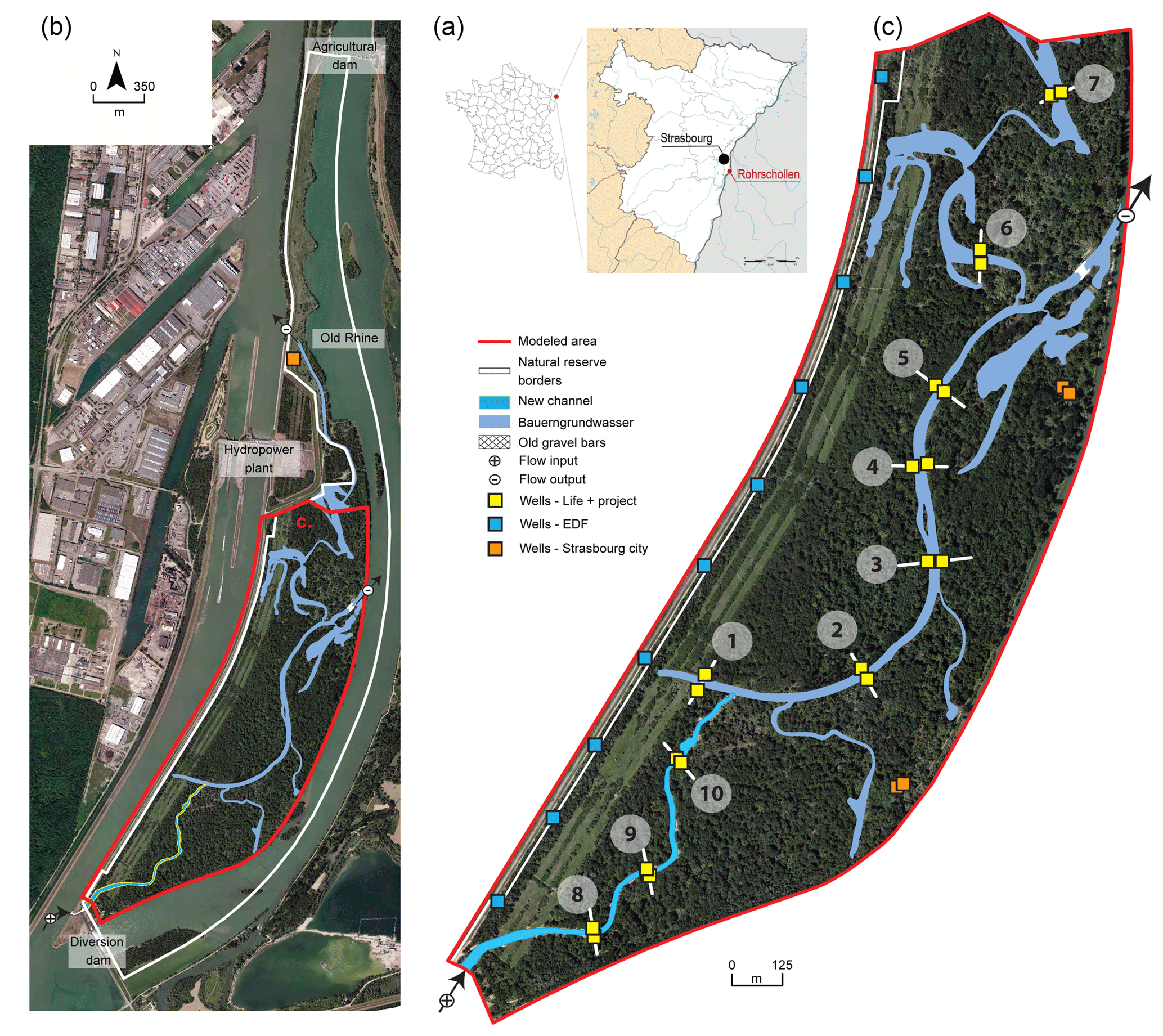
Figure 1 (a) Location of the studied area (France), (b) aerial view of Rohrschollen Island, and (c) network of hydrologic response measurements (mainly hydraulic heads and water fluxes).

In this paper, the low-dimensional integrated hydrologic model NIHM (for Normally Integrated Hydrologic Model) is applied to the restored hydrosystem of Rohrschollen Island, which is an artificial island located 8 km south of Strasbourg (Upper Rhine, France; see Fig. 1a). Previous studies have shown that the hydrological, sedimentological, and geomorphological dynamics of the island were very active due to intense hyporheic exchanges and surface processes (Eschbach et al., 2017, 2018). These dynamics were tightly linked to the flood dynamics of the Rhine river that were progressively lost because of territorial developments along the Rhine fluvial corridor. A restoration project started in 2012 with the idea of improving the overall functioning of the ecosystem through artificial injections. The restoration actions specifically target short-term enhancement of hyporheic exchanges over the whole island and the reactivation of sediment transport in the main channel of the island. Even though short-term horizon effects are the main target of the restoration, it is expected that duplicating flooding episodes over time in the island could result in beneficial impacts on the long-term ecological and biological health of the island.

The proposed study addresses and models a couple of these flooding episodes with the four main objectives that are (i) to test the performance of NIHM regarding the description of highly transient hydrologic behavior over short periods of time; (ii) to check on the correspondences and discrepancies between model results and TIR imaging in the delineation of exfiltration patterns; (iii) to investigate the efficiency of restoration actions undertaken at Rohrschollen Island, especially regarding surface–subsurface water exchanges, and (iv) to propose optimal short-term management procedures regarding the enhancement of surface–subsurface exchanges.

It could be argued that short-term analysis of a restored system does not fit the general understanding stating that restoration processes are intended to render benefits over long-term horizons. In the present case (but also in many other cases), restoration works are recent and the system is still evolving. This means that long-term simulations on the basis of the actual settings of the system would probably miss its further evolution. It makes sense to assess the behavior of a recently restored hydrosystem in response to short-terms events. Duplicating calculations for various short stress periods is also a way to foresee how the system could behave, even though uncertainty and model robustness associated with the evolution of the system over time persist. This study is limited to the analysis of the short-term response (to flood events that are also pulse stresses) of a transient hydrosystem via a highly resolved model in time and space.

2 Data and hydrological modeling

2.1 Study area – Rohrschollen Island

2.1.1 General description

Rohrschollen Island is the result of historical engineering works carried out along the Rhine river mainly to prevent flooding and to develop navigation and agriculture. The hydrological and geomorphological dynamics of the area were massively impacted (Eschbach et al., 2017, 2018). Three structures completely control the current geometry and hydraulic behavior of Rohrschollen Island (Fig. 1): (a) the diversion dam (built in 1970) at the southern end of the island that diverts most of the river flow into the Rhine Canal at the western bank of the island, (b) the hydropower plant (built in 1970) located on the Rhine Canal downstream of Rohrschollen Island, and (c) an agricultural dam (built in 1984) at the northern part of the island to keep a constant water level in the by-passed Old Rhine at the eastern bank of Rohrschollen Island.

Rohrschollen Island was regularly flooded in the past (Eschbach et al., 2018). The main anastomosed channel inside the island, the Bauerngrundwasser (BGW; Fig. 1), was disconnected on its upstream mouth from the Rhine river by the excavation of the Rhine Canal. This disconnection, combined with dampened groundwater dynamics along the island, impacted the hydrological, geomorphological, and ecological functioning of the hydrosystem (Eschbach et al., 2017). The former flood dynamics induced large water table fluctuations, lively interactions between the surface and subsurface domains, intense rejuvenation of habitat mosaic driven by geomorphological processes, and a high level of biodiversity for species of aquatic and riverine habitats. As a result of engineering works performed to control the Rhine river, the ecological services associated with the flood dynamics and the hydrologic connection between the floodplain of the island and the river were lost.

In 2012, the European Union funded a restoration project (LIFE + program) in order to counteract the loss of various natural processes and thus re-establish part of the former dynamics of the system. The Rhine river water is now injected through a floodgate into a 900 m long new artificial channel (south of the island; Fig. 1b) following rules that relate the injected discharge with the discharge of the Rhine river. A constant discharge of 2 m³ s⁻¹ – later referred to as the base flow injection – is injected when the discharge of the Rhine river does not exceed 1550 m³ s⁻¹. When the discharge of the Rhine river rises above this value, the injected discharge is increased accordingly up to a maximum rate of 80 m³ s⁻¹. These injections should contribute to (a) enhancing discharge into the surface water bodies of the island (especially in the BGW) and partly recovering floods on the island (floods occur when the injected rate exceeds the top-edge discharge of the new channel at 20 m³ s⁻¹), (b) recovering bedload transport and lateral channel dynamics (especially along the new channel), (c) activating surface–subsurface interactions, and (d) stimulating the renewal of aquatic and riverine ecosystems. Overall, it is worth noting that the hydrologic behavior of Rohrschollen Island is primarily controlled by water levels in the Old Rhine and the Rhine Canal (regulated by the two dams and the hydropower plant mentioned above) and by the injection discharge in the new channel.

2.1.2 Hydrologic monitoring

A large interdisciplinary environmental monitoring was conducted to investigate the effects and the efficiency of the restoration, but also to check on some risks such as the eventual collapsing of the new channel banks under strong water injections. As an example, a dense network of piezometers (yellow squares in Fig. 1c) was installed along both the artificial new channel and the BGW. More precisely, 10 transects along these channels were instrumented with a piezometer on each channel bank. The time resolution of measurements in the 20 piezometers ranges from 5 min along the new channel to 10 min along the BGW. This network is particularly crucial for hydrological model calibration and to understand the interactions between groundwater and surface water bodies. Other subsurface head measurements are also available on the eastern and western sides of the island. The French national electricity company (EDF) is operating devices at the western side of the island (along the Rhine Canal) to monitor the state of the dike road (blue squares in Fig. 1c) and, as the owner and manager of the Rohrschollen Island Nature Reserve, the city of Strasbourg is following subsurface water table dynamics at the eastern side (orange squares in Fig. 1c).

2.1.3 Historical and sedimentological surveys

Geohistorical and sedimentological surveys were used to reconstruct the morpho-sedimentary temporal trajectory of the island since the middle of the 18th century. The geohistorical survey is partly based on six old maps, two sets of aerial photographs, and the actual digital elevation model of the island (see Fig. 2a). Planimetric data were georeferenced in a GIS (geographic information system) and processed to highlight the temporal dynamics of the main morpho-ecological units. The sedimentological study was based on seven coring transects distributed along the BGW. Grain size analysis was also performed on sediment samples from three transects and two pits in the floodplain to determine the transport and deposition processes of fine sediments. The combination of the geohistorical and sedimentological analysis helped to reconstruct the sedimentary deposition trajectory and to locate precisely historical gravel bars (see Fig. 2b). This information was used to spatialize the parameters of the hydrological model and to preset the initial values of key parameters related to the composition of the sediment units. More details on this part of the study can be found in Eschbach et al. (2018).

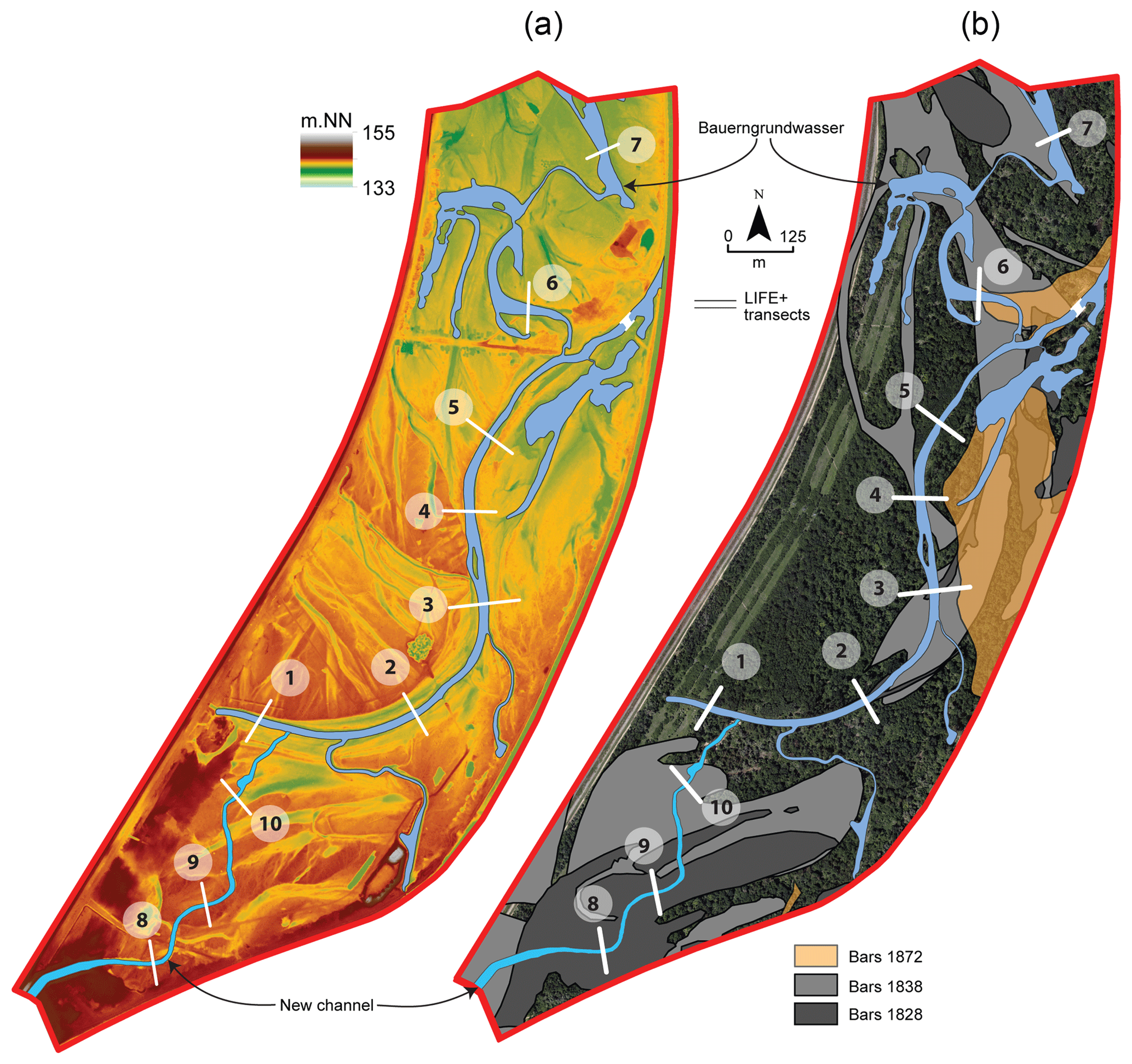
Figure 2 Digital elevation model of Rohrschollen Island (a) and location of the main gravel bars reconstructed from the geohistorical and sedimentological studies (b). The black and white lines correspond to transects of hydrologic measurements (see Fig. 1).

2.1.4 Thermal infrared imaging

Thermal infrared (TIR) imaging was carried out at Rohrschollen Island to investigate the relationship between the evolution of some geomorphological features (e.g., riffles and pools) and the interactions between surface and subsurface waters. A FLIR b425 infrared camera was fixed under a paraglider to take pictures covering the whole island. The camera was calibrated using several key parameters such as water emissivity and the height above the topography. The flight took place on 22 January 2015, a date chosen to have minimal canopy extension and maximal temperature contrast between surface and subsurface waters (with approximately 4 ^∘C surface temperature and 10 ^∘C groundwater temperature). The thermal images were processed to locate thermal anomalies along the new artificial channel and the BGW. The radiance was first converted into temperature using Planck's law and in situ measurements as references. The temperature maps were then georeferenced, and pixels associated with high uncertainty on temperatures were also discarded. Further treatments based on optic images (in the visible wavelengths) delineated and located surface objects such as banks, vegetation, logjams, and gravel bars. Further details about thermal image processing can be found in Eschbach et al. (2017).

2.2 Hydrological modeling strategy

2.2.1 The Normally Integrated Hydrologic Model (NIHM)

The integrated hydrological model used to model Rohrschollen Island is the Normally Integrated Hydrologic Model (NIHM) (Pan et al., 2015; Weill et al., 2017; Jeannot et al., 2018). This tool is a physically based and spatially fully distributed model that describes flow processes in the surface and subsurface domains of a catchment and their couplings. For the sake of simplicity, only the model parts used for this study are presented here. A detailed presentation of the model (primarily concerning treatment of the flow equations) is available, for example, in Jeannot et al. (2018).

The subsurface flow processes are described using a low-dimensional equation that results from the integration of the 3-D Richards equation along a direction normal to the bedrock (i.e., the impervious bottom of the aquifer). The final equation for subsurface flow can be written as

$$\begin{array}{}\text{(1)}& {\displaystyle }{\displaystyle \frac{\partial \stackrel{\mathrm{‾}}{\mathit{\theta }}}{\partial t}}+\stackrel{\mathrm{‾}}{S}\left(h\right){\displaystyle \frac{\partial h}{\partial t}}+{\mathrm{\nabla }}_{x,y}\cdot \left(-\stackrel{\mathrm{‾}}{T}\left(\mathit{\theta }\right){\mathrm{\nabla }}_{x,y}h\right)=Q_{\mathrm{w}},\end{array}$$

where $\stackrel{\mathrm{‾}}{\mathit{\theta }}\left(h\right)=\underset{z_{\mathrm{w}}}{\overset{z_{\mathrm{s}}}{\int }}\mathit{\theta }\left(z\right)\mathrm{d}z$, $\stackrel{\mathrm{‾}}{S}\left(h\right)=S_{\mathrm{sat}}h$, $\stackrel{\mathrm{‾}}{T}(h$, $\mathit{\theta })=K_{\mathrm{sat}}h+\underset{z_{\mathrm{w}}}{\overset{z_{\mathrm{s}}}{\int }}K(\mathit{\theta }\left(z\right))\mathrm{d}z$. K_sat and S_sat are averages along the integration direction z of the saturated hydraulic conductivity tensor and the specific storage capacity in the saturated zone, respectively. θ (–) is the water content, K (L T⁻¹) is the tensor of hydraulic conductivity, h (L) is the hydraulic head (or the capillary head), and Q_w (L T⁻¹) is a source term that accounts for the subsurface interactions with both the 1-D river network and the 2-D overland flow. It is worth noting that the 1-D river network compartment was not used in this study because the precision of the digital elevation model (Fig. 2a) was enough to delineate and model streams, channels, and other small water routing in slight topographic depressions of the 2-D overland flow layer.

The 2-D overland flow layer is described using the so-called diffusive wave equation, which is written as

$$\begin{array}{ll}{\displaystyle \frac{\partial \left(h_{\mathrm{s}}+z_{\mathrm{s}}\right)}{\partial t}}& {\displaystyle }-{\mathrm{\nabla }}_x\cdot \left(T_{\mathrm{s},x}{\mathrm{\nabla }}_x\left(h_{\mathrm{s}}+z_{\mathrm{s}}\right)\right)\\ \text{(2)}& {\displaystyle }& {\displaystyle }-{\mathrm{\nabla }}_y\cdot \left(T_{\mathrm{s},x}{\mathrm{\nabla }}_y\left(h_{\mathrm{s}}+z_{\mathrm{s}}\right)\right)=q,\end{array}$$

with

$${\displaystyle }{\displaystyle }{T}_{\mathrm{s},x}={\displaystyle \frac{h_{\mathrm{s}}^{\mathrm{5}/\mathrm{3}}}{N_{\mathrm{man},x}^{\mathrm{2}}\mathit{\beta }\mathrm{\nabla }\left(h_{\mathrm{s}}+z_{\mathrm{s}}\right)}};T_{\mathrm{s},y}={\displaystyle \frac{h_{\mathrm{s}}^{\mathrm{5}/\mathrm{3}}}{N_{\mathrm{man},y}^{\mathrm{2}}\mathit{\beta }\mathrm{\nabla }\left(h_{\mathrm{s}}+z_{\mathrm{s}}\right)}}$$

$$\begin{array}{ll}{\displaystyle }\mathit{\beta }\mathrm{\nabla }\left(h_{\mathrm{s}}+z_{\mathrm{s}}\right)=& {\displaystyle }\left[{\left({\displaystyle \frac{\partial \left(h_{\mathrm{s}}+z_{\mathrm{s}}\right)}{\partial x}}\right)}^{\mathrm{2}}{\displaystyle \frac{\mathrm{1}}{N_{\mathrm{man},x}^{\mathrm{4}}}}+{\left({\displaystyle \frac{\partial \left(h_{\mathrm{s}}+z_{\mathrm{s}}\right)}{\partial y}}\right)}^{\mathrm{2}}\right.\\ {\displaystyle }& {\displaystyle }{\left.{\displaystyle \frac{\mathrm{1}}{N_{\mathrm{man},y}^{\mathrm{4}}}}\right]}^{\mathrm{1}/\mathrm{4}}.\end{array}$$

h_s (L) is the water depth at the surface; z_s (L) is the soil surface elevation; u_x and u_y (L T⁻¹) are the water velocity components along the x and y directions (that are locally defined in the plane normal to the direction of integration z of Eq. 1); q (L T⁻¹) is a source term including the exchanges with the 1-D river flow compartment and with the subsurface; and N_man,x and N_man,y (L${}^{-\mathrm{1}/\mathrm{3}}$ T) are the Manning coefficients in the x and y directions, respectively.

The coupling between Eqs. (1) and (2) relies upon a first-order law stating that the flux exchanged between surface and subsurface flows is proportional to the head gradient between the two compartments. The exchanged flux $Q_{\mathrm{Ex},\mathrm{2}\mathrm{D}\leftrightarrow \mathrm{SS}}$ (L T⁻¹) can be formalized as

$$\begin{array}{}\text{(3)}& {\displaystyle }& {\displaystyle }{Q}_{\mathrm{Ex},\mathrm{2}\mathrm{D}\leftrightarrow \mathrm{SS}}=K_{\mathrm{Int}}{\displaystyle \frac{\left(z_{\mathrm{s}}+h_{\mathrm{s}}\right)-h}{l_{\mathrm{e}}}}{F}_{\mathrm{s}},\text{(4)}& {\displaystyle }& {\displaystyle }{F}_{\mathrm{s}}=\min \left[{\left({\displaystyle \frac{h_{\mathrm{s}}}{h_{\mathrm{ob}}}}\right)}^{\mathrm{2}\left(\mathrm{1}-h_{\mathrm{s}}/h_{\mathrm{ob}}\right)};\mathrm{1}\right],\end{array}$$

where K_Int (L T⁻¹) is the vertical hydraulic conductivity at the interface between the surface and subsurface compartments, l_e is a user-defined coupling length (i.e., an empirical thickness of the interface between surface and subsurface compartments), F_s (–) is a scaling function accounting for the saturated–unsaturated character of the interface between the surface and subsurface, and h_ob is the total obstruction height accounting for small irregularities of the topography.

Regarding the numerical solution, both equations are solved together in a fully implicit manner using advanced numerical schemes. Note that both equations are two-dimensional and that only one computation mesh mimicking the topographic surface of the system is required for simulating both surface and subsurface processes, including their interactions. It is worth noting that employing a partly simplified model is an incentive to the duplication of calculations, as is necessary for example when solving inverse problems, evaluating model sensitivities, and testing hypotheses. This possibility is not exploited in this study which can be seen as a test of feasibility to capture the short-term very transient dynamics of a hydrological system via a model highly resolved in time and space. Simulations discussed below take between 5 and 24 h of calculation (for simulation times of 7 to 45 days, respectively) on a single core of a modern processor. Duplicating calculations for the purposes mentioned above remains tractable by distributing the calculation load over multiple cores.

2.2.2 Model setup and parametrization

The computation mesh for all the simulations of the study was built from data from an airborne lidar survey performed in 2015 that produced high-resolution images of the topography (50 cm in the horizontal plane and 1–2 cm in elevation). The whole Rohrschollen Island is meshed using triangular elements of 20 m on a side. The exception is a 120 m wide corridor surrounding the new channel and the BGW where a refined spatial resolution of 10 m is used. The higher resolution is assumed to better capture the hydrological dynamics and the surface–subsurface interactions along the surface water bodies of the island.

As mentioned previously, the two key drivers of the hydrological response at Rohrschollen Island are (i) the water levels in the Old Rhine and the Rhine Canal and (ii) the discharge injected in the artificial channel. In base flow conditions, the routine value of 2 m³ s⁻¹ as the injected discharge brings the equivalent of 20 m of annual rainfall over the whole island. Moreover, the water table in the island is always fed by the Old Rhine and the Rhine Canal, reducing considerably the potential effect of evapotranspiration on piezometric levels. Provided that the time horizon of the simulations is rather short (less than 50 days), the meteorological forcing – i.e., rainfall and evapotranspiration – is thus considered negligible in the study. Prescribed-head (Dirichlet) boundary conditions are imposed at the western and eastern banks of Rohrschollen Island for the subsurface model, and they have been documented by measurements collected by the EDF and the city of Strasbourg. These boundary conditions may vary over time, depending on the modeled period and availability of data. The northern and southern parts of the island were considered as no-flow boundaries. The initial conditions were set up by running the model with consistent boundary conditions for the subsurface and the base flow injection rate of 2 m³ s⁻¹ at the new channel inlet until stable hydrological conditions were reached.

Several exploratory calculations were performed by varying a single parameter one at the time to obtain some kind of rough sensitivity analysis. A rigorous sensitivity analysis would have required the analytical differentiation of the state variable derivatives with respect to model parameters, which was out of the scope of a study mainly testing whether hydrological modeling would be suited to quantify the effects of restoration works. These exploratory calculations showed us that the model was mainly sensitive to the values of saturated hydraulic conductivity and the exchange coefficient between the surface and subsurface. The calculations also showed us that the other parameters, for example the Manning coefficient, were less sensitive. Therefore, only the saturated hydraulic conductivity and the exchange coefficient were considered as variable in space while the other parameters were supposed uniform over the whole island. The initial spatial distribution of the saturated hydraulic conductivity and the exchange coefficient mainly relies upon patterns drawn from the geohistorical and sedimentological surveys of the island (Eschbach et al., 2018). As an example, Fig. 2 maps three historical snapshots of the main geomorphological units (gravel bars). Corridors around the new channel, the BGW, and the network of paleo-channels visible in the floodplain (see the digital elevation model in Fig. 2) were defined and parametrized separately to account for specific deposition histories resulting in specific sediment grain size. Both the saturated hydraulic conductivity and the exchange coefficient were considered as uniform over zones (subareas) of the modeled domain (a block-heterogeneous system), and the initial spatial delineation of these zones was processed via a GIS.

Results from particle size laboratory analysis were used to define the initial values of the hydraulic conductivity, the retention curve parameters of the sediments, and the exchange coefficient between the surface and subsurface. Sediment cores were taken along the artificial channel and the BGW at different depths and locations when the piezometric network of the island was installed. The samples were then analyzed in the lab to determine their textural and particle size characteristics. The Rosetta model (US Salinity Lab, Riverside, CA) was then used to relate textural properties of soils with the model parameters. Regarding Manning's coefficient, the initial values for the artificial channel and the BGW were set following standard tables and field observations.

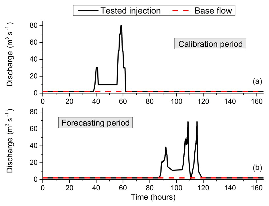
Figure 3 Evolution over time of flow rates injected in the new artificial channel feeding Rohrschollen Island during the period selected for calibrating the integrated hydrological model (a) and the period chosen as a validation (forecasting) exercise (b).

2.2.3 Model calibration and validation

The integrated model was calibrated and validated using two periods of time for which high-rate injections in the new artificial channel were carried out. The first period (9–15 December 2014) was used as a model calibration exercise which encompassed two peaks of injection with one reaching 80 m³ s⁻¹. The second selected period (15–21 May 2015) was employed as a validation exercise with three injection peaks, two of them exceeding 70 m³ s⁻¹. In both cases, peak injections superimpose onto a continuous base flow fed by the routine injection of 2 m³ s⁻¹ in the inlet channel. Figure 3 reports the evolution of the injected flow rates over time at the system inlet for both the calibration and validation periods.

Table 1 List of parameters that were calibrated with initial and final value after calibration. Only the saturated hydraulic conductivity and the exchange coefficient were considered variable in space. The other parameters are considered homogeneous for the whole simulated domain.

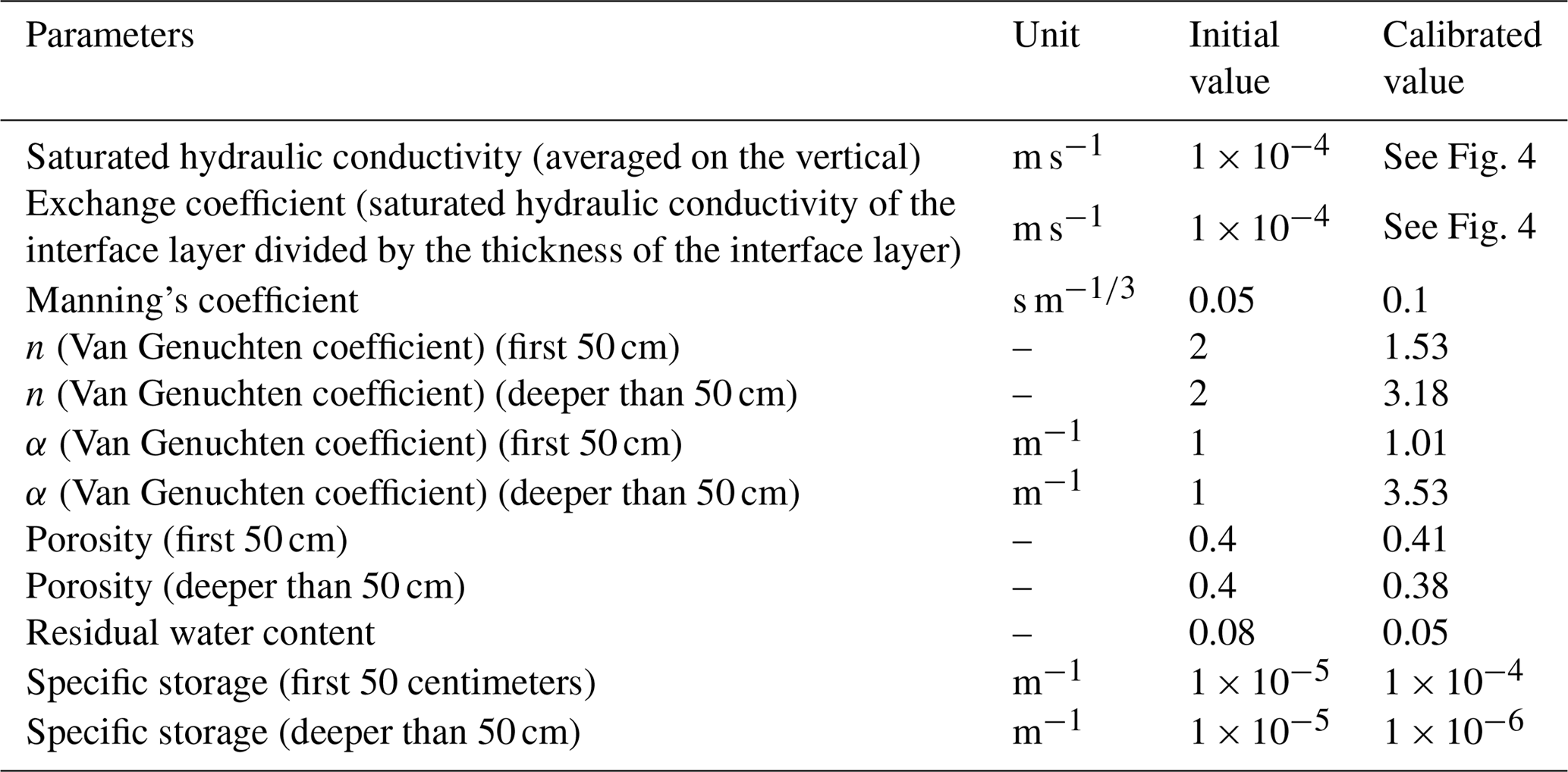
After a first simulation employing the initial parametrization (defined in Sect. 2.2.2), all the parameters were manually calibrated to match up to the simulated head levels in the subsurface with observations. Both the root mean square error (RMSE) and the Kling–Gupta efficiency (KGE) associated with observed heads at the 10 transects cross-cutting the new channel and the BGW were used as indicators to evaluate the quality of the simulations. Table 1 gathers the initial and optimal (i.e., after calibration) parameter values, showing that – except for the saturated hydraulic conductivity, the exchange coefficient, and the Van Genuchten parameters of the deeper part of the subsurface – the optimal parameters are very close to the initial ones. During the calibration process, the initial spatial zonation was also modified even if the preservation of the main spatial units initially defined was attempted. More precisely, a few additional zones were delineated, mainly along the new channel and the BGW to account for partly clogged zones that showed delayed or smoothed responses of subsurface heads to infiltration. Figure 4 maps the final set of parameters for the saturated hydraulic conductivity and the exchange coefficient. The sets of calibrated parameters were then used for simulating the validation period to check whether the calculated subsurface head levels match up to the measured values.

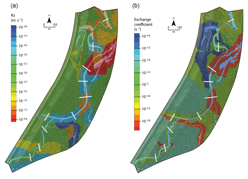
Figure 4 Calibrated fields of saturated hydraulic conductivity in the subsurface compartment (a) and exchange coefficient between surface and subsurface compartments (b).

It is worth noting here that the calibration exercise was performed over a period where the TIR images were not available, which means, in turn, that the calibration only relied upon measured groundwater head levels as a reference. The goal of the calibration was not to match the exfiltration patterns identified through the TIR imaging. When this information became available, the simulation period used for the calibration was extended to reach the date of the airborne flight (22 January 2015), and the boundary conditions were updated. The exfiltration patterns were then used as verification information to confirm that the model could properly describe the interactions between surface and subsurface and thus be used as a forecasting tool. Forecasts discussed hereinafter cover optimizations of injections in the artificial channel upstream of the island, which are mainly supposed to maintain active ponding and wetlands (mainly from groundwater outcrops) over long periods.

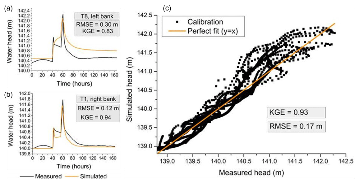
Figure 5 Comparison between simulated and measured hydraulic heads in the subsurface during the calibration period. (a, b) Evolution over time at the two transects, that is, the worst (a) and best (b) transects regarding RMSE. (c) Local in space and time values of simulated hydraulic heads as a function of observed ones. RMSE is the root mean square error, and KGE is the Kling–Gupta efficiency.

3 Results and discussion

3.1 Model outputs

Figure 5 displays the evolution over time of simulated and observed piezometric heads at two locations (transects) in the island. It also plots simulated versus observed heads for all locations and sampling times used during the calibration period. Heads at transects in Fig. 5 were selected to show the best and worst match concerning RMSE between simulation and observation. It is worth noting that, before injections peaks, the simulated heads are mainly influenced by the Dirichlet-type boundary conditions on the east and west sides of the island. Few data (one measure each 15 days) were available to set up these Dirichlet boundary conditions, and the almost-constant-over-time simulated heads before peak injections do not fully match up to the head transients observed along the BGW. That being said, in general the model adequately reproduces the system dynamics, capturing the two peaks of head response associated with the injection patterns at the new channel inlet. The recession part of the response is also captured well with a slight overestimation of the final head value for transect T8 (Fig. 5a). The plot of simulated versus observed heads (Fig. 5c) confirms that the model tends to overestimate the piezometric heads as more points are located above the 1:1 straight line. This feature is associated with one of the founding assumptions of the model regarding the vadose zone, which is integrated with the saturated zone and can be excessively or not sufficiently capacitive, depending on the mean soil moisture (see Weill et al., 2017). The values of the two performance indicators that are the RMSE and the KGE are satisfying, at 17 cm and 0.93, respectively. Regarding the KGE value of all measured versus simulated heads, the Pearson correlation coefficient is 0.97, the bias ratio is 1, and the variance ratio is 1.07.

Figure 6 depicts the same information as Fig. 5 but for the validation period. The agreement between simulated and measured heads remains good with an RMSE of 24 cm and a KGE of 0.75, associated with a Pearson correlation coefficient of 0.94, a bias ratio of 1, and a variance ratio of 1.24. The decrease in the KGE values from calibration to validation steps does not generate bias between observed and simulated head values. Nevertheless, the variance ratio slightly increases, showing that errors between observed and simulated heads also increase from calibration to validation. That being said, both exercises show that the NIHM and its calibrated set of parameters render convincing simulations of the highly transient hydrologic behavior of the system.

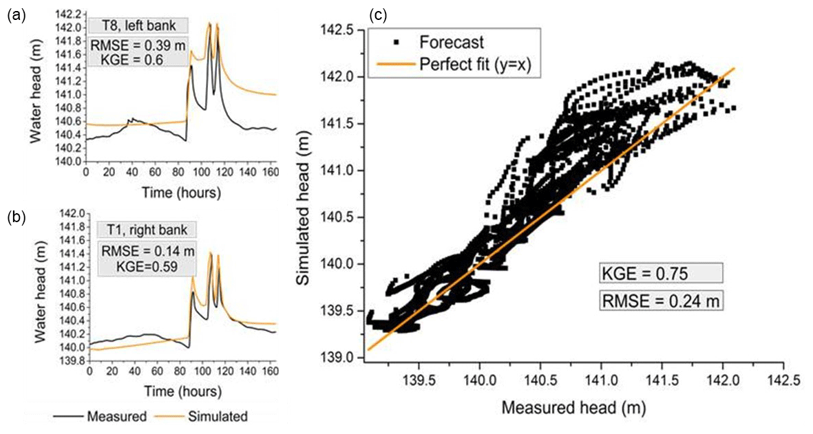
Figure 6 Comparison between simulated and measured hydraulic heads in the subsurface during the validation period. (a, b) Evolution over time at the two transects, that is, the worst (a) and best (b) transects regarding RMSE. (c) Local in space and time values of simulated hydraulic heads as a function of observed ones. RMSE is the root mean square error, and KGE is the Kling–Gupta efficiency.

3.2 Interactions between surface and subsurface in Rohrschollen Island

Once calibration and validation were completed, the ability to capture the interactions between surface and subsurface was checked by comparing the modeled exfiltration patterns simulated on 22 January 2015 with the thermal anomalies identified via airborne TIR imaging performed the same day (see Sect. 2). In Fig. 7, the thermal anomalies are represented as pink spots, and the simulated exfiltration patterns are represented as colored patches ranging from blue to red as a function of the exfiltration rate. Figure 7 focuses on the area of the island where a vast majority of the thermal anomalies were identified. The simulated exfiltration patterns usually coincide with the thermal anomalies from the TIR, even though their spatial extension may be wider than thermal anomalies. This feature can be the consequence of multiple factors, such as (a) the substantial sedimentary heterogeneity of the streambed not sufficiently represented in the model, (b) a spatial resolution of the computation mesh not fine enough to capture the very small-scale surface–subsurface interactions, and (c) the measurement uncertainty plaguing the TIR analysis. Keeping these approximations in mind, the hydrologic model correctly locates the surface–subsurface interactions in the island and provides flux values that are not accessible via TIR surveys.

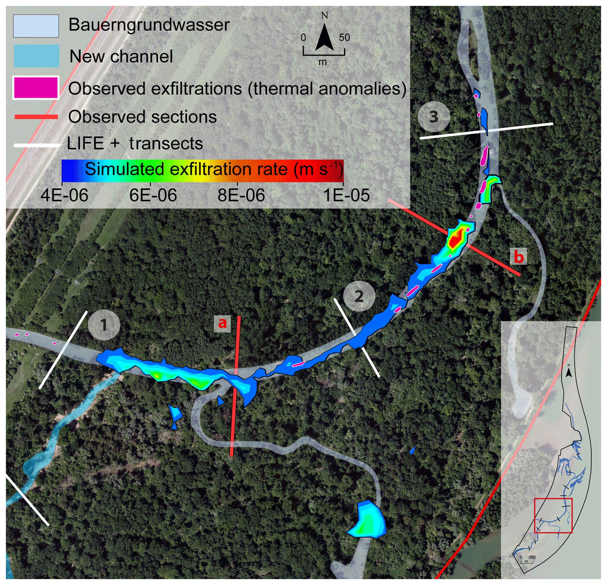
Figure 7 Comparison between simulated exfiltration patterns and thermal anomalies identified via thermal infrared imaging close to the junction between the new channel (southeast corner) and the BGW (Bauerngrundwasser; center of figure). Red transects a and b are locations where surface water and groundwater head are followed to exemplify surface–subsurface interactions in Fig. 9.

Given that a rigorous sensitivity analysis to model parameters was not undertaken, it could be stated that flawed model parameter values are at the origin of mismatches between TIR images and the exfiltration zones modeled by NIHM. Nevertheless, the macroscopic hydraulic diffusion (the ratio of conductivity to specific storage) is correctly fitted as shown by the good match of observed heads both in time and amplitude. The point is that thermal anomalies are visible at a scale on the order of less than 10 m, which is also the scale of local heterogeneity of clay, sand, gravel, and pebble deposits in alluvial systems. A numerical model handling local heterogeneity at that scale should employ a mesh of 1–2 m resolution. In view of the available data, building this model is unfeasible, except by conjecturing the distribution of hydraulic parameters (as can be done for example in stochastic approaches to the inverse problem). The lack of data suggests that perfect accuracy cannot be expected, and the mismatch between the measurement and model resolutions is the main reason for discrepancies between TIR and model delineation of exfiltration zones. In addition and under the present modeling constraints, we suggest that the quality of model results does not relate to the fact that the model accurately represents data over a single scenario, but rather to the fact that it roughly represents data over multiple different scenarios (events). Unfortunately, we only had one single set of TIR imagery at our river reach.

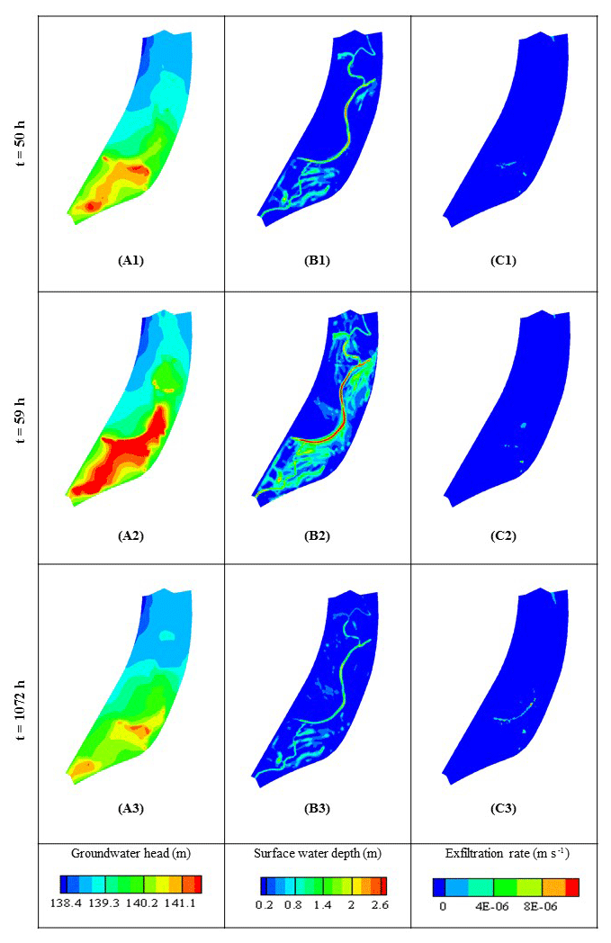
Figure 8 Groundwater head, surface water thickness, and exfiltration rate over the whole of Rohrschollen Island for three different periods (in hours after the beginning of injection) of the calibration period. Notably, the last period is also the date of the airborne thermal infrared imaging.

Figures 8 and 9 picture the transient interactions between surface and subsurface and tell us why the banana-shaped exfiltration zone reported in Fig. 7 is close to the junction of the new artificial channel and the BGW. Figure 8 displays maps of the groundwater head, the surface water thickness, and the exfiltration rates over the whole island at three different times of the calibration period that are t=50 h (i.e., after the first injection peak), t=59 h (i.e., at the second injection peak), and t=1072 h (i.e., the date of the airborne TIR flight). As evidenced by the snapshots of groundwater head and surface water thickness, the water injected upstream of the island, flowing into the BGW, its dead ends, and the associated floodplain, rapidly infiltrates, producing an important increase in groundwater levels alongside the new artificial channel (and also the BGW), which had been excavated but was still not clogged with fine sediments. When the maximum injection rate is reached (t=59 h), surface ponding occurs on a significant portion of the island and the groundwater mounding invades all the upstream part of the BGW. Note that the exfiltration rates (Fig. 8, right panels) are localized in small topographic depressions during the injection period, and the banana-shaped exfiltration pattern (Fig. 7) is still inactive. The latter pattern only appears during the recession period (t=1072 h) when the strong injection rates have stopped. It appears alongside the BGW in the vicinity of the area where the groundwater level previously increased the most. Figure 9 represents cross sections along locations a and b in Fig. 7 for t=59 and t=1072 h and reports on the subsurface water head, the surface water elevation (set to the topography elevation when surface water thickness is zero), and infiltration–exfiltration rates. It shows that (a) the topography mainly controls the banana-shaped infiltration–exfiltration zone (depressions in Fig. 9) and (b) the temporal dynamics and amplitude of exfiltration are the combined effect of surface water rapidly flowing toward the system outlet (i.e., surface water thickness diminishes) and a slow recession of the groundwater heads after the main peaks of injected flow rates have vanished.

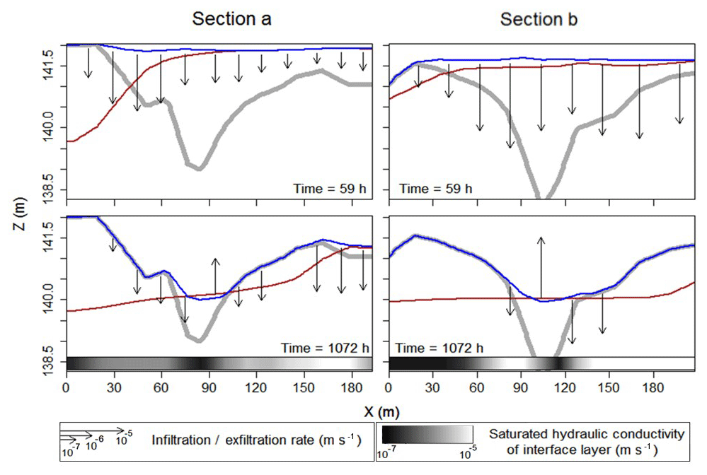
Figure 9 Evolution of surface water elevation (blue), groundwater head (red), and exchange fluxes (arrows) along transects a and b (located in Fig. 7) at two periods (hours after the beginning of injection) of the calibration period. A thick grey line represents the topographic profile. The grey scale indicates values of the saturated hydraulic conductivity at the interface between surface and subsurface.

Figure 10 reports on the evolution over time of the total infiltration and exfiltration fluxes calculated over the whole surface area of the island during the two-peak calibration period. While the injection rate is kept at 2 m³ s⁻¹, both infiltration and exfiltration fluxes are stable with much more infiltration than exfiltration. When the injected flow rate increases, the infiltrated flux follows a slightly delayed evolution over time, which is very similar to the injection hydrograph (with a two-peak shape; see Fig. 3). Meanwhile, as the hydraulic gradient between surface and subsurface changes at some locations, the exfiltration decreases in areas that turn from an exfiltration to an infiltration regime due to excess of surface water associated with injection peaks. Once the injection of water into the new artificial channel stops, the infiltration flux sharply decreases while the exfiltration flux increases. An exfiltration peak can be observed just at the end of the recession period. It is noteworthy that, during the recession period, the exfiltration flux is almost constant over time and kept at a value twice that observed before injection (Fig. 10). In the end, forced water injections at the new channel inlet foster water exfiltration from the subsurface that maintains ponds and wetlands on the surface over long periods (say, approximately 15 days for each injection, as simulated by the model but not reported in Fig. 10).

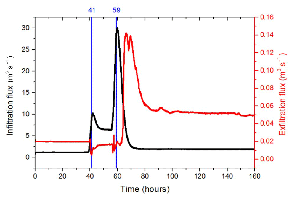
Figure 10 Evolution of the infiltration and exfiltration volumetric fluxes during the first steps of the calibration period (where evolutions are essential).

3.3 Efficiency of the restoration actions

One of the issues targeted in this study is the assessment of the efficiency of hydrological restoration projects. The previous results indicate that water injections in the new channel enhance the interactions between surface and subsurface compartments of the island, noting that it was observed during the excavation that the new channel had been dug in highly conductive sedimentary formations. It may be interesting to check via a modeling approach what causes differences between the current restored circumstances and a pre-restoration situation. As the pre-restored island is not well documented in terms of hydraulic data, we considered a scenario where the pre-restored island is similar to the current situation (including, e.g., geometry and boundary conditions) with the exception that the newly excavated channel connecting Rohrschollen Island's BGW and the Rhine river is absent. Therefore, no forced injection may occur at the southern boundary of the pre-restored island. The hydrological behavior of the pre-restored situation has been simulated and compared with an actual case where the injection rate in the new channel is at the usual year-round configuration of 2 m³ s⁻¹.

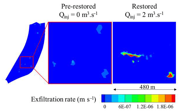
Figure 11 Patterns of exfiltration for the pre-restored and the restored situations. The focus is on the most active zone of Rohrschollen Island regarding surface–subsurface interactions.

Figure 11 displays snapshots of exfiltration rates in a subarea of the island for the pre-restored and the restored scenarios. Even with an injected flow rate of 2 m³ s⁻¹, both the exfiltration surfaces and exfiltration rates are much higher in the restored situation. In other words, the base flow regime of the restored situation is sufficient to positively impact the interactions between surface and subsurface compartments of the island. When forced injections enhance the development of wetlands and maintain high rates of exfiltration over long periods, from the mere hydrological standpoint, restoration works are successful.

3.4 Suggestions for management practices

The injection scenarios tested in the hydrological model with maximum peaks reaching 80 m³ s⁻¹ are designed as a routine inlet for feeding Rohrschollen Island with water, but some other inlet procedures can also be considered to improve the functioning of the island. We analyzed with the hydrological model how these routine injections could be designed to maximize either the spatial extension of exfiltration areas maintaining wetlands in surface or the time over which exfiltration occurs. Two hypothetical injections superimposed to a base flow of 2 m³ s⁻¹ in the new channel were proposed, with the first one being of short duration (24 h) with an injection rate of 15 m³ s⁻¹ and the second one being of longer duration (120 h) but with a weaker injection rate of 5 m³ s⁻¹ (see Fig. 12a). As the total injected water volume differs between both scenarios (the weaker injection flushes almost twice the volume of the stronger injection), it can also be determined which of the two configurations – high rate–small volume or small rate–high volume – maximizes the extension and/or duration of exfiltration.

Figure 12 (a) Injection rates of two scenarios seeking optimal exfiltration surface areas and durations at Rohrschollen Island. (b) Evolution over time of excess or lack of exfiltration surface area compared with exfiltration surface produced by a routine injection rate of 2 m³ s⁻¹ at the inlet of the system.

Figure 12b plots the excess or lack of exfiltration surface areas during injections compared with surface areas sustained by base flow (2 m³ s⁻¹) in the new channel. The evolution over time of these excess exfiltration areas (or lack thereof) occurs for both injection scenarios with a lack of exfiltration areas occurring during the injection periods when infiltration from the surface dominates. After the injection peak is completed, the recession period – starting at t=52 h for the high injection rate and t=162 h for the small injection rate (Fig. 12) – always shows an excess of exfiltration areas. The interesting point is that the high injection rate delivers a smaller volume of water in the system but maintains increased areas of exfiltration over extensive periods. For its part, the small injection rate has no effect beyond t=250 h with a system coming back to its initial state with 2 m³ s⁻¹ of routine injection at the inlet. Finally, injecting less volume but with high injection rates over short periods is better suited to maintaining exfiltration over long periods as the process feeding wetlands on the island (Fig. 12). It is also likely (though not studied in this work) that intense injections favor the unclogging of the BGW, which are the primary surface water routes contributing to water renewal on the island.

As already mentioned, the short-term behavior of the hydrosystem in response to flood events motivated this study. In a context where long-term horizons of the restoration benefits are the principal objective, performing short-term simulations does not depart from this prescribed objective. The exploration of injection scenarios discussed above with a model highly resolved in time and space deciphers how the system currently behaves. Duplicating that kind of simulations could for example inform on the number and intensity of flood events needed to maintain a prescribed number of exfiltration days (and mean flow rates) in a year. In that sense, modeling short-term events in not necessarily in complete opposition to long-term considerations on the modeled system.

4 Conclusions

Restoration projects to counterbalance the undesired effects of anthropogenic actions on the hydrological, geomorphological, and ecological status of riverine ecosystems have recently spread worldwide. As the interactions between surface and subsurface compartments of the hydrosystem have a strong impact on hydrological, biogeochemical, and ecological processes, it makes sense to rely upon integrated hydrological modeling when addressing the question of restoration efficiency. When feasible (i.e., with tractable problems and models), hydrological modeling with high resolution in time and space can accurately delineate infiltration–exfiltration areas and their evolution over time as key factors for maintaining active surface river networks

Relying upon simplified models, not in their physics but rather on their dimensionality (as done in the present study), renders many problems tractable and calculable. This is the case with Rohrschollen Island, which shows smooth variations of topography that do not help to locate ground water outcrops. This comment also extends to the very transient hydraulic behaviors requiring refined time steps to accurately capture temporal evolutions of the system.

If the focus is placed on infiltration–exfiltration patterns as a reliable indicator of the effects of restoration in riverine systems, any spatially distributed modeling exercise needs conditioning regarding both model inputs and outputs. Concerning the conditioning (or control) of model outputs associated with the delineation of exfiltration areas, the recent technique of airborne, low-altitude, and high-resolution thermal infrared imaging is very promising. The technique is not free of measurement errors and artifacts, but it has been shown reliable enough to highlight interactions between surface and subsurface compartments of the hydrosystem that coincide with simulations. Further investigations should duplicate thermal imaging over time with the aim of grasping the transient behavior of surface–subsurface interactions and discussing the best versus the worst environmental conditions where imaging is applicable.

Rohrschollen Island (and many other fluvial hydrosystems) is very specific regarding surface–subsurface interactions, meaning that water heads in the aquifer are often close to surface water levels. This means that slight variations in both compartments may invert the direction of exchanged fluxes between compartments. In that case, injecting significant volumes of water in a system to store them over large periods may be counterproductive, even though these volumes may contribute to flooding over large areas. Large volumes are diverted into the rapidly flowing surface water and exit the system. Intense injections of smaller volumes over short periods foster intense local infiltration into the subsurface. The subsequent water mounding in the aquifer then results in long-term storage and smooth release of water via exfiltration. This behavior, hardly foreseeable, was that simulated for Rohrschollen Island and could also apply to many other configurations of fluvial corridors. These results show that management rules for a restored system may be developed from modeling exercises handling various forcing scenarios applied to the system. If it is accepted that exfiltration (sustaining ponding and wetlands) is a valuable indicator of riverine restoration, additional works should envision various settings to improve this process. For example, it is not clear if several smaller inlets could replace a single inlet in the system for higher efficiency. Is water extraction from the surface and reinjection in the subsurface a valuable process that can generate slow exfiltration over broad areas? Physically based integrated modeling of hydrosystems might propose some answers.